Parallel-plate and spherical capacitors in Born-Infeld electrostatics: An analytical study

Abstract

In 1934, Max Born and Leopold Infeld suggested and developed a nonlinear modification of Maxwell electrodynamics, in which the electrostatic self-energy of an electron was a finite value. In this paper, after a brief introduction to Lagrangian formulation of Born-Infeld electrodynamics with an external source, the explicit forms of Gauss’s law and the electrostatic energy density in Born-Infeld theory are obtained. The capacitance and the stored electrostatic energy for a parallel-plate and spherical capacitors are computed in the framework of Born-Infeld electrostatics. We show that the usual relations $U=\frac{1}{2}C_{{}_{\textrm{Maxwell}}}(\triangle\phi)^{2}$ and $U=\frac{q^{2}}{2C_{{}_{\textrm{Maxwell}}}}$ are not valid for a capacitor in Born-Infeld electrostatics. Numerical estimations in this research show that the nonlinear corrections to the capacitance and the stored electrostatic energy for a capacitor in Born-Infeld electrostatics are considerable when the potential difference between the plates of a capacitor is very large.

Keywords: Classical field theories; Classical electromagnetism; Other special classical field theories; Nonlinear or nonlocal theories and models

PACS: 03.50.-z, 03.50.De, 03.50.Kk, 11.10.Lm

1 Introduction

As we know, Maxwell electrodynamics is a very successful theory which is able to describe a wide range of macroscopic phenomena in classical electricity and magnetism. Unfortunately, in Maxwell electrodynamics the electric field of a point charge $q$ at the position of the point charge and the classical self-energy of a point charge are infinite, i.e.,

$$\textbf{E}(\textbf{x}) = \frac{q}{4\pi\epsilon_{0}|\textbf{x}|^{2}}\frac{\textbf{x}}{|\textbf{x}|}\;\stackrel{{\scriptstyle|\textbf{x}|\rightarrow 0}}{{-\!\!-\!\!\!\longrightarrow}}\infty,$$ (1a)

$$U = \frac{q^{2}}{8\pi\epsilon_{0}}\int^{\infty}_{0}\frac{d|\textbf{x}|}{|\textbf{x}|^{2}}\rightarrow\infty.$$ (1b)

More than 80 years ago, Max Born and Leopold Infeld suggested a nonlinear modification of Maxwell electrodynamics [1]. The Lagrangian density of Born-Infeld electrodynamics is not only Lorentz invariant, but also depends on the gauge potential and its first derivative. In contrast with the Maxwell Lagrangian density, the Born-Infeld Lagrangian density contains quartic and higher-order powers of the electromagnetic field tensor [1-7]. In Born-Infeld electrodynamics, the classical self-energy of a point charge like electron is a finite value [1]. In ref. [8], the authors have proposed a non-Abelian generalization of Born-Infeld theory from the viewpoint of non-commutative geometry. Recent studies in string theory show that the low-energy dynamics of a $D9$-brane, induced by the quantum theory of the open strings attached to it, can be described by the following action [9-13]:

$$S_{{}_{\textrm{BI}}}=\frac{1}{(4\pi^{2}\alpha^{\prime})^{5}g_{{}_{s}}}\;\int d^{10}x\sqrt{-det_{{}_{{}_{{}_{\begin{subarray}{c}\!\!\!\!\!\!\!\!\!\mu,\nu\end{subarray}}}}}\big{(}\eta_{\mu\nu}+T^{-1}F_{\mu\nu}\big{)}},$$ (2)

where $\alpha^{\prime}$ is the “universal Regge slope”, $g_{{}_{s}}$ is the “string coupling constant”, $T=\frac{1}{2\pi\alpha^{\prime}}$ is the “string tension”, and $F_{\mu\nu}$ is the “field strength of the gauge fields living on the $D9$-brane worldvolume” (see ref. [13]). In ref. [13], Szabo has shown that for a pure electric field configuration the absolute value of the electric field in action (2) can not go beyond the maximum value $E_{{}_{c}}=T=\frac{1}{2\pi\alpha^{\prime}}$. In ref. [14], the Lagrangian formulation of Born-Infeld electrodynamics coupled to an axionic field in the presence of an external source has been studied. The electric field and the stored electrostatic energy per unit length for an infinite charged line and an infinitely long cylinder in Born-Infeld electrostatics have been calculated analytically in ref. [15]. The black hole solutions of Einstein’s gravity in the presence of different models of nonlinear electrodynamics in a $3+1$-dimensional space-time have been studied in refs. [16-20]. Another interesting theory of nonlinear electrodynamics was suggested and developed by German physicists in 1930s [21-23]. Heisenberg and his students Euler and Kockel showed that classical electrodynamics must be corrected by nonlinear terms due to the vacuum polarization effects [21-28]. The Heisenberg-Euler-Kockel effective Lagrangian density is given by [21-28]

$${\cal L}_{{}_{\textrm{HEK}}}=\underbrace{\frac{1}{2}\big{(}\epsilon_{0}\textbf{E}^{2}-\frac{\textbf{B}^{2}}{\mu_{0}}\big{)}}_{Maxwell\;term}+\underbrace{\frac{2\alpha^{2}\hbar^{3}\epsilon_{0}^{2}}{45m_{e}^{4}c^{5}}\Big{[}\big{(}\textbf{E}^{2}-c^{2}\textbf{B}^{2}\big{)}^{2}+7c^{2}(\textbf{E}.\textbf{B})^{2}\Big{]}}_{one-loop\;corrections}+...\;,$$ (3)

where $m_{e}$ is the electron mass, and $\alpha=\frac{e^{2}}{4\pi\epsilon_{0}\hbar c}$ is the fine structure constant. The general expression for effective Lagrangian density of quantum electrodynamics can be written as follows:

$${\cal L}=\sum_{i=0}^{\infty}\sum_{j=0}^{\infty}c_{{}_{i,j}}F^{i}G^{j},$$ (4)

where $F:=\big{(}\epsilon_{0}\textbf{E}^{2}-\frac{\textbf{B}^{2}}{\mu_{0}}\big{)}$ and $G:=\sqrt{\frac{\epsilon_{0}}{\mu_{0}}}(\textbf{E}.\textbf{B})$ are two Lorentz invariant quantities, and $c_{{}_{i,j}}$ are model-dependent constant parameters [24]. It should be mentioned that the Heisenberg-Euler-Kockel effective Lagrangian density in eq. (3) is a very special case of eq. (4). In refs. [29,30], the authors have suggested a new generalization of Maxwell electrodynamics which is known as logarithmic electrodynamics. These authors have proved that the classical self-energy of a point charge in logarithmic electrodynamics is a finite value. In ref. [31], the author has suggested a new model of nonlinear electrodynamics with three independent parameters, in which the static electric self-energy of point-like particles is finite. In 2013, another generalization of nonlinear electrodynamics was proposed, which is known as exponential electrodynamics [32]. The black hole solutions of Einstein’s gravity coupled to exponential electrodynamics in a $3+1$-dimensional space-time have been obtained in ref. [32]. In ref. [33] and independently in ref. [34], the authors have suggested a nonlinear generalization of Maxwell electrodynamics, in which the electric field of a point charge is singular at the position of the point charge but the classical self-energy of the point charge has a finite value. In ref. [35], a novel model for nonlinear electrodynamics has been proposed which violates the gauge symmetry. This model describes charged particles with finite electrostatic self-energy. Nowadays, theoretical physicists believe that the concept of a point charge is only an idealization. The measurement of the anomalous magnetic moment of an electron leads to the following upper bound on the size of the electron $l$ [36]: $l\leq 10^{-17}\;\textrm{cm}.$ According to the above statements a point charge like an electron could be considered as an extended object with a finite size. The existence of an effective radius for the electron leads to a finite electrostatic self-energy. In ref. [37], the author has shown that the stored energy in a nonlinear capacitor with a voltage-dependent capacitance does not satisfy the usual relation $U=\frac{1}{2}C_{{}_{\textrm{Maxwell}}}(\triangle\phi)^{2}$. The electric field between the plates of a parallel-plate capacitor and the magnetic field around a long straight wire carrying a current $i$ have been calculated in the framework of Heisenberg-Euler-Kockel electrodynamics [38]. Finally, the concept of duality in Born-Infeld electrodynamics has been studied by Gibbons and Rasheed [39]. This paper is organized as follows. In sect. 2, the Lagrangian formulation of Born-Infeld electrodynamics with an external source is presented. We obtain the explicit forms of Gauss’s law and the energy density of an electrostatic field for Born-Infeld electrostatics. In sect. 3, the capacitance and the stored electrostatic energy for a parallel-plate capacitor are calculated nonperturbatively in the framework of Born-Infeld theory. In sect. 4, we determine the capacitance and the stored electrostatic energy for a spherical capacitor and an isolated sphere in Born-Infeld electrostatics. Numerical estimations in sect. 5 show that the nonlinear corrections to the capacitance and the stored electrostatic energy for a capacitor in Born-Infeld theory are negligible when the potential difference between the plates of a capacitor is small. The metric of space-time has the signature $(+,-,-,-)$.

2 Lagrangian formulation of Born-Infeld electrodynamics with an external source

The Lagrangian density for Born-Infeld electrodynamics in a 3+1-dimensional space-time is [1]

$${\cal L}_{{}_{\textrm{BI}}}=\epsilon_{0}\beta^{2}\bigg{\{}1-\sqrt{1+\frac{c^{2}}{2\beta^{2}}F_{\mu\nu}F^{\mu\nu}-\frac{c^{4}}{16\beta^{4}}\big{(}F_{\mu\nu}\,\star F^{\mu\nu}\big{)}^{2}}\bigg{\}}-J^{\mu}A_{\mu},$$ (5)

where $F_{\mu\nu}=\partial_{\mu}A_{\nu}-\partial_{\nu}A_{\mu}$ is the electromagnetic field tensor, $\star F^{\mu\nu}=\frac{1}{2}\epsilon^{\mu\nu\alpha\beta}F_{\alpha\beta}$ is the dual field tensor, and $J^{\mu}=(c\rho,\textbf{J})$ is an external source for the $U(1)$ gauge field $A^{\mu}=(\frac{1}{c}\phi,\textbf{A})$ [6,39,40]. The parameter $\beta$ in eq. (5) is called the Born-Infeld parameter. This parameter shows the upper limit of the electric field in Born-Infeld electrodynamics. In the limit $\beta\longrightarrow\infty$, eq. (5) reduces to the following Lagrangian density:

$${\cal L}_{{}_{\textrm{BI}}}|_{{}_{large\;\beta}}={\cal L}_{{}_{\textrm{M}}}+\frac{c^{2}}{32\mu_{0}\beta^{2}}\bigg{[}\big{(}F_{\mu\nu}\,\star F^{\mu\nu}\big{)}^{2}+\big{(}F_{\mu\nu}F^{\mu\nu}\big{)}^{2}\bigg{]}+{\cal O}(\beta^{-4}),$$ (6)

where ${\cal L}_{{}_{\textrm{M}}}=-\frac{1}{4\mu_{0}}F_{\mu\nu}F^{\mu\nu}-J^{\mu}A_{\mu}$ is the Maxwell Lagrangian density [40]. The Euler-Lagrange equation for the gauge field $A_{\lambda}$ is

$$\frac{\partial{\cal L}_{{}_{\textrm{BI}}}}{\partial A_{\lambda}}-\partial_{\rho}\bigg{(}\frac{\partial{\cal L}_{{}_{\textrm{BI}}}}{\partial(\partial_{\rho}A_{\lambda})}\bigg{)}=0.$$ (7)

If we substitute eq. (5) into eq. (7), we will obtain the inhomogeneous Born-Infeld equations as follows:

$$\partial_{\rho}\bigg{(}\frac{F^{\rho\lambda}-\frac{c^{2}}{4\beta^{2}}\big{(}F_{\mu\nu}\star F^{\mu\nu}\big{)}\star F^{\rho\lambda}}{\sqrt{1+\frac{c^{2}}{2\beta^{2}}F_{\mu\nu}F^{\mu\nu}-\frac{c^{4}}{16\beta^{4}}\big{(}F_{\mu\nu}\star F^{\mu\nu}\big{)}^{2}}}\bigg{)}=\mu_{0}J^{\lambda}.$$ (8)

Using the definition of the electromagnetic field tensor, we obtain the following identity:

$$\partial_{\mu}F_{\nu\lambda}+\partial_{\nu}F_{\lambda\mu}+\partial_{\lambda}F_{\mu\nu}=0.$$ (9)

Equation (9) is known as the Bianchi identity. In 3+1-dimensional space-time, the components of $F_{\mu\nu}$ and $\star F^{\mu\nu}$ can be written as follows:

$$F_{\mu\nu} = \left({\begin{array}[]{cccc}0&\frac{E_{x}}{c}&\frac{E_{y}}{c}&\frac{E_{z}}{c}\\ -\frac{E_{x}}{c}&0&-B_{z}&B_{y}\\ -\frac{E_{y}}{c}&B_{z}&0&-B_{x}\\ -\frac{E_{z}}{c}&-B_{y}&B_{x}&0\end{array}}\right),$$ (14)

$$\star F^{\mu\nu} = \left({\begin{array}[]{cccc}0&-B_{x}&-B_{y}&-B_{z}\\ B_{x}&0&\frac{E_{z}}{c}&-\frac{E_{y}}{c}\\ B_{y}&-\frac{E_{z}}{c}&0&\frac{E_{x}}{c}\\ B_{z}&\frac{E_{y}}{c}&-\frac{E_{x}}{c}&0\end{array}}\right).$$ (19)

Using eqs. (10) and (11), eqs. (8) and (9) can be written in the vector form as follows:

$$\boldsymbol{\nabla}\cdot\textbf{D}(\textbf{x},t) = \rho(\textbf{x},t),$$ (20)

$$\boldsymbol{\nabla}\times\textbf{H}(\textbf{x},t) = \textbf{J}(\textbf{x},t)+\frac{\partial\textbf{D}(\textbf{x},t)}{\partial t},$$ (21)

$$\boldsymbol{\nabla}\cdot\textbf{B}(\textbf{x},t) = 0,$$ (22)

$$\boldsymbol{\nabla}\times\textbf{E}(\textbf{x},t) = -\frac{\partial\textbf{B}(\textbf{x},t)}{\partial t},$$ (23)

where $\textbf{D}(\textbf{x},t)$ and $\textbf{H}(\textbf{x},t)$ are given by

$$\textbf{D}(\textbf{x},t) = \epsilon_{0}\frac{\textbf{E}(\textbf{x},t)+\frac{c^{2}}{\beta^{2}}\big{(}\textbf{E}(\textbf{x},t).\textbf{B}(\textbf{x},t)\big{)}\textbf{B}(\textbf{x},t)}{\sqrt{1-\frac{1}{\beta^{2}}\bigg{(}\textbf{E}^{2}(\textbf{x},t)-c^{2}\textbf{B}^{2}(\textbf{x},t)\bigg{)}-\frac{c^{2}}{\beta^{4}}\big{(}\textbf{E}(\textbf{x},t).\textbf{B}(\textbf{x},t)\big{)}^{2}}},$$ (24)

$$\textbf{H}(\textbf{x},t) = \frac{1}{\mu_{0}}\frac{\textbf{B}(\textbf{x},t)-\frac{1}{\beta^{2}}\big{(}\textbf{E}(\textbf{x},t).\textbf{B}(\textbf{x},t)\big{)}\textbf{E}(\textbf{x},t)}{\sqrt{1-\frac{1}{\beta^{2}}\bigg{(}\textbf{E}^{2}(\textbf{x},t)-c^{2}\textbf{B}^{2}(\textbf{x},t)\bigg{)}-\frac{c^{2}}{\beta^{4}}\big{(}\textbf{E}(\textbf{x},t).\textbf{B}(\textbf{x},t)\big{)}^{2}}}.$$ (25)

Now, let us consider the electrostatic case where $\textbf{B}=\textbf{J}=0$ and all other quantities are independent of time. In this case the classical Born-Infeld equations (12)-(15) are

$$\boldsymbol{\nabla}\cdot\bigg{(}\frac{\textbf{E}(\textbf{x})}{\sqrt{1-\frac{\textbf{E}^{2}(\textbf{x})}{\beta^{2}}}}\bigg{)} = \frac{\rho(\textbf{x})}{\epsilon_{0}},$$ (26)

$$\boldsymbol{\nabla}\times\textbf{E}(\textbf{x}) = 0.$$ (27)

Equations (18) and (19) are fundamental equations of Born-Infeld electrostatics [3,15]. Using the divergence theorem, we obtain the integral form of eq. (18) as follows:

$$\oint_{S}\frac{1}{\sqrt{1-\frac{\textbf{E}^{2}(\textbf{x})}{\beta^{2}}}}\;\textbf{E}(\textbf{x}).\textbf{n}\;da=\frac{1}{\epsilon_{0}}\int_{V}\rho(\textbf{x})d^{3}x,$$ (28)

where $V$ is the three-dimensional volume enclosed by a two-dimensional surface $S$. Equation (20) is Gauss’s law in Born-Infeld electrostatics [15]. The symmetrized energy-momentum tensor for Born-Infeld electrodynamics in eq. (5) is [1,41]

$$T^{\sigma}_{\;\tau}=-\frac{1}{\mu_{0}\Omega}\bigg{(}F^{\sigma\lambda}-\frac{c^{2}}{4\beta^{2}}\big{(}F_{\mu\nu}\star F^{\mu\nu}\big{)}\star F^{\sigma\lambda}\bigg{)}F_{\tau\lambda}+\epsilon_{0}\beta^{2}(\Omega-1)\delta^{\sigma}_{\;\tau},$$ (29)

where $\Omega$ is defined as follows:

$$\Omega:=\sqrt{1+\frac{c^{2}}{2\beta^{2}}F_{\mu\nu}F^{\mu\nu}-\frac{c^{4}}{16\beta^{4}}\big{(}F_{\mu\nu}\star F^{\mu\nu}\big{)}^{2}}.$$ (30)

Using eqs. (10) and (11) together with eq. (21), the energy density of an electrostatic field in Born-Infeld electrodynamics is given by

$$u(\textbf{x})=T^{0}_{\;0}(\textbf{x})=\epsilon_{0}\beta^{2}\bigg{(}\frac{1}{\sqrt{1-\frac{\textbf{E}^{2}(\textbf{x})}{\beta^{2}}}}-1\bigg{)}.$$ (31)

It is necessary to note that for large values of $\beta$, the modified electrostatic energy density in eq. (23) becomes the usual electrostatic energy density in Maxwell electrodynamics, i.e.,

$$u(\textbf{x})|_{{}_{large\;\beta}}=\frac{1}{2}\epsilon_{0}\textbf{E}^{2}(\textbf{x})+{\cal O}(\beta^{-2}).$$ (32)

3 Capacitance of a parallel-plate capacitor in Born-Infeld electrostatics

Let us consider two large parallel conducting plates with area $A$ and separation $d$ (see fig. 1).

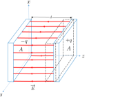
Figure 1: A parallel-plate capacitor. The Gaussian surface is represented by dashed lines. $\,\hat{\textbf{e}}_{z}$ is the unit vector in the $z$-direction.

Using the modified Gauss’s law in eq. (20), the electric field for the Gaussian surface in fig. 1 becomes

$$\textbf{E}(\textbf{x}) = \frac{q}{\epsilon_{0}A}\frac{1}{\sqrt{1+\big{(}\frac{q}{\beta\epsilon_{0}A}\big{)}^{2}}}\,(-\hat{\textbf{e}}_{z})$$

$$= -\frac{q}{\epsilon_{0}A}\,\hat{\textbf{e}}_{z}+\frac{q^{3}}{2\beta^{2}\epsilon_{0}^{3}A^{3}}\,\hat{\textbf{e}}_{z}+{\cal O}(\beta^{-4}).$$ (33)

The first term on the right-hand side of eq. (25) shows the uniform electric field between the plates of a parallel-plate capacitor in Maxwell electrostatics, while the second and higher order terms in eq. (25) show the effect of nonlinear corrections. Now, let us calculate the potential difference $\triangle\phi$ between the plates of a parallel-plate capacitor in Born-Infeld electrostatics. Equation (19) implies that the electrostatic field $\textbf{E}(\textbf{x})$ can be written as follows:

$$\textbf{E}(\textbf{x})=-\boldsymbol{\nabla}\phi(\textbf{x}),$$ (34)

where $\phi(\textbf{x})$ is the electrostatic potential. Equation (26) leads to the following formula:

$$\phi_{f}-\phi_{i}=-\int^{f}_{i}\textbf{E}(\textbf{x}).d\textbf{l},$$ (35)

where $d\textbf{l}$ is an infinitesimal displacement vector. If we use eqs. (25) and (27), we will obtain the following expression for $\triangle\phi$:

$$\triangle\phi = \phi_{+}-\phi_{-}$$

$$= -\int_{-}^{+}\frac{q}{\epsilon_{0}A}\frac{1}{\sqrt{1+(\frac{q}{\beta\epsilon_{0}A})^{2}}}(-\,\hat{\textbf{e}}_{z}).(\hat{\textbf{e}}_{z}\,dz)$$

$$= \frac{qd}{\epsilon_{0}A}\frac{1}{\sqrt{1+(\frac{q}{\beta\epsilon_{0}A})^{2}}}.$$ (36)

We know that the amount of charge on each plate of a capacitor and the potential difference between the plates of a capacitor are proportional to each other, i.e.,

$$q=C\,\triangle\phi,$$ (37)

where $C$ is the capacitance of the capacitor. Note that eq. (29) has been used to determine the capacitance of nonlinear capacitors [12,37,38]. If eq. (28) is inserted into eq. (29), the capacitance of a parallel-plate capacitor in Born-Infeld electrostatics becomes

$$C_{{}_{\textrm{BI}}}=\frac{\epsilon_{0}A}{d}\sqrt{1+(\frac{q}{\beta\epsilon_{0}A})^{2}}.$$ (38)

Using eqs. (28) and (30) the above expression for $C_{{}_{BI}}$ can be rewritten as follows:

$$C_{{}_{\textrm{BI}}}=\frac{C_{{}_{\textrm{M}}}}{\sqrt{1-(\frac{\triangle\phi}{\phi_{\,\textrm{critical}}})^{2}}},$$ (39)

where $C_{{}_{\textrm{M}}}=\frac{\epsilon_{0}A}{d}$ is the capacitance of a parallel-plate capacitor in Maxwell electrostatics, and $\phi_{\,\textrm{critical}}:=\beta d$ is the critical potential difference. Equation (31) shows that the capacitance of a parallel-plate capacitor in Born-Infeld electrostatics depends on the potential difference between the plates of the capacitor. It should be noted that the determination of $C_{{}_{\textrm{BI}}}$ in eq. (31), has been mentioned as an unsolved exercise in Zwiebach’s book [12]. As we know the capacitance of a capacitor is a real positive parameter. According to the above statement $\triangle\phi$ in eq. (31) must satisfy the following inequality:

$$\triangle\phi<\phi_{\textrm{\,critical}}.$$ (40)

The above inequality has an interesting physical interpretation. The potential difference between the plates of a parallel-plate capacitor in Born-Infeld electrostatics can not go beyond the critical potential difference $\phi_{\,\textrm{critical}}$. Now, we want to calculate the stored electrostatic energy density between the plates of a parallel-plate capacitor in Born-Infeld electrostatics. By putting eq. (25) in eq. (23), we obtain

$$u(\textbf{x})=\epsilon_{0}\beta^{2}\Big{\{}\sqrt{1+(\frac{q}{\beta\epsilon_{0}A})^{2}}-1\Big{\}}.$$ (41)

Using eq. (33), the stored electrostatic energy between the plates of a parallel-plate capacitor in Born-Infeld electrostatics according to fig. 1 is given by

$$U = \int_{{area\;of\;a\;plate}}da\;\int_{0}^{d}dz\,u(\textbf{x})$$

$$= \epsilon_{0}\beta^{2}\Big{\{}\sqrt{1+(\frac{q}{\beta\epsilon_{0}A})^{2}}-1\Big{\}}\,Ad.$$ (42)

If we use eq. (28), we can rewrite eq. (34) as follows:

$$U = C_{{}_{\textrm{M}}}\,\phi^{2}_{\,\textrm{critical}}\bigg{\{}\Big{[}1-\big{(}\frac{\triangle\phi}{\phi_{\,\textrm{critical}}}\big{)}^{2}\Big{]}^{-\frac{1}{2}}-1\bigg{\}}$$

$$= \underbrace{\frac{1}{2}\;C_{{}_{\textrm{M}}}(\triangle\phi)^{2}}_{Maxwell\;term}+\underbrace{\frac{3}{8}\;C_{{}_{\textrm{M}}}\;\frac{(\triangle\phi)^{4}}{\phi^{2}_{\,\textrm{critical}}}}_{first-order\;nonlinear\;correction}+\underbrace{{\cal O}(\phi^{-4}_{\,\textrm{critical}})}_{higher-order\;nonlinear\;corrections}.$$ (43)

Equation (35) shows that the expression $U=\frac{1}{2}\;C_{{}_{\textrm{M}}}(\triangle\phi)^{2}$ is not valid for a parallel-plate capacitor in Born-Infeld electrostatics.

4 Spherical capacitor in Born-Infeld electrostatics

In this section we want to determine the capacitance of a spherical capacitor in Born-Infeld electrostatics. Let us consider two concentric spherical conductors of radii $a$ and $b$ (see fig. 2).

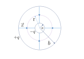
Figure 2: The Gaussian surface for a spherical capacitor. The spherical symmetry of the problem implies that $\textbf{E}(\textbf{x})=E_{r}(r)\,\hat{\textbf{e}}_{r}$, where $\hat{\textbf{e}}_{r}$ is the radial unit vector in spherical coordinates $(r,\theta,\varphi)$.

Using the spherical symmetry of the problem together with the modified Gauss’s law in eq. (20), the electric field between the plates of a spherical capacitor becomes

$$\textbf{E}(\textbf{x})=\frac{q}{4\pi\epsilon_{0}r^{2}}\frac{1}{\sqrt{1+(\frac{q}{4\pi\epsilon_{0}\beta r^{2}})^{2}}}(-\,\hat{\textbf{e}}_{r})\;;a<r<b.$$ (44)

Using eqs. (27) and (36), the potential difference between the plates of a spherical capacitor in Born-Infeld electrostatics can be determined as follows:

$$\triangle\phi = \phi_{+}-\phi_{-}$$

$$= \int_{a}^{b}\frac{q}{4\pi\epsilon_{0}r^{2}}\frac{1}{\sqrt{1+(\frac{q}{4\pi\epsilon_{0}\beta r^{2}})^{2}}}dr$$

$$= \frac{q}{4\pi\epsilon_{0}}\Big{\{}(\frac{1}{a}-\frac{1}{b})-\frac{1}{10}s^{4}(\frac{1}{a^{5}}-\frac{1}{b^{5}})+\frac{1}{24}s^{8}(\frac{1}{a^{9}}-\frac{1}{b^{9}})+{\cal O}(s^{12})\Big{\}},$$ (45)

where $s:=(\frac{q}{4\pi\epsilon_{0}\beta})^{\frac{1}{2}}$ is a constant positive parameter with dimension $length$. After inserting eq. (37) into eq. (29), we obtain

$$C_{{}_{\textrm{BI}}} = 4\pi\epsilon_{0}\,\frac{ab}{b-a}\bigg{\{}1+\frac{1}{10}s^{4}\frac{b^{5}-a^{5}}{a^{4}b^{4}(b-a)}+\frac{1}{4}s^{8}\frac{1}{a^{8}b^{8}(b-a)}$$

$$\Big{[}\frac{1}{25}\frac{(b^{5}-a^{5})^{2}}{(b-a)}-\frac{1}{6}(b^{9}-a^{9})\Big{]}+{\cal O}(s^{12})\bigg{\}}.$$ (46)

Substitution of eq. (36) into eq. (23) yields the following expression for the electrostatic energy density between the plates of a spherical capacitor

$$u(\textbf{x})=\epsilon_{0}\beta^{2}\bigg{\{}\sqrt{1+\big{(}\frac{s}{r}\big{)}^{4}}-1\bigg{\}}.$$ (47)

Using the above equation, the total stored energy in spherical capacitor is given by

$$U = 4\pi\epsilon_{0}\beta^{2}\,\int_{a}^{b}r^{2}\bigg{\{}\sqrt{1+\big{(}\frac{s}{r}\big{)}^{4}}-1\bigg{\}}dr$$

$$= \frac{q^{2}}{8\pi\epsilon_{0}}\frac{b-a}{ab}\bigg{\{}1-\frac{1}{20}s^{4}\frac{b^{5}-a^{5}}{a^{4}b^{4}(b-a)}+\frac{1}{72}s^{8}\frac{b^{9}-a^{9}}{a^{8}b^{8}(b-a)}+{\cal O}(s^{12})\bigg{\}}.$$ (48)

If we use eqs. (37), (38), and (40), the potential, capacitance, and total energy for an isolated spherical conductor of radius $R$ can be determined as follows:

$$\lim_{b\rightarrow\infty}\;\lim_{a\rightarrow R}\;\triangle\phi=\frac{q}{4\pi\epsilon_{0}R}\bigg{\{}1-\frac{1}{10}(\frac{s}{R})^{4}+\frac{1}{24}(\frac{s}{R})^{8}+{\cal O}\Big{(}(\frac{s}{R})^{12}\Big{)}\bigg{\}},$$ (49)

$$\lim_{b\rightarrow\infty}\;\lim_{a\rightarrow R}\;C_{{}_{\textrm{BI}}}=4\pi\epsilon_{0}R\bigg{\{}1+\frac{1}{10}(\frac{s}{R})^{4}-\frac{19}{600}(\frac{s}{R})^{8}+{\cal O}\Big{(}(\frac{s}{R})^{12}\Big{)}\bigg{\}},$$ (50)

$$\lim_{b\rightarrow\infty}\;\lim_{a\rightarrow R}\;U=\frac{q^{2}}{8\pi\epsilon_{0}R}\bigg{\{}1-\frac{1}{20}(\frac{s}{R})^{4}+\frac{1}{72}(\frac{s}{R})^{8}+{\cal O}\Big{(}(\frac{s}{R})^{12}\Big{)}\bigg{\}}.$$ (51)

Equations (38) and (42) show that the capacitance of a spherical capacitor in Born-Infeld electrostatics depends on the amount of charge on each plate of the capacitor.

5 Summary and conclusions

Today, we know that the classical self-energy of a point charge has an infinite value in Maxwell electrodynamics. In 1934, Max Born and Leopold Infeld introduced a nonlinear generalization of Maxwell electrodynamics, in which the classical self-energy of an electron was a finite value [1]. In Born-Infeld electrodynamics the absolute value of the electric field can not go beyond the critical electric field $\beta$, i.e., $|\textbf{E}|\leq\beta$. Born and Infeld attempted to calculate $\beta$ by equating the classical self-energy of the electron in their theory with its rest mass energy. They obtained the following numerical value for $\beta$ [1]:

$$\beta_{{}_{\textrm{Born-Infeld}}}=1.2\times 10^{20}\frac{\textrm{V}}{\textrm{m}}.$$ (52)

In 1973, Gerhard Soff and his coworkers obtained a new lower bound on $\beta$ [42]. This lower bound on $\beta$ was

$$\beta_{{}_{\textrm{Soff}}}\geq 1.7\times 10^{22}\frac{\textrm{V}}{\textrm{m}}.$$ (53)

In a recent paper about photonic processes in Born-Infeld theory, Davila et al. [43] have obtained the following lower bound on $\beta$:

$$\beta_{{}_{\textrm{Davila}}}\geq 2.0\times 10^{19}\frac{\textrm{V}}{\textrm{m}}.$$ (54)

It is interesting to note that the lower bound in eq. (46) is near to the $\beta_{{}_{\textrm{Born-Infeld}}}$ in eq. (44). In this paper, after a brief introduction to the Lagrangian formulation of Born-Infeld electrodynamics in the presence of an external source, the capacitance of parallel-plate and spherical capacitors have been calculated analytically in the framework of Born-Infeld electrostatics. According to eqs. (30), (31), (38), and (42) the capacitance of a capacitor in Born-Infeld electrostatics depends on the amount of charge on each plate of the capacitor. Using the relation $C_{{}_{\textrm{M}}}=\frac{\epsilon_{0}A}{d}$, eq. (34) can be rewritten as follows:

$$U = \beta^{2}d^{2}C_{{}_{\textrm{M}}}\Big{\{}\big{[}1+\big{(}\frac{q}{\beta dC_{{}_{\textrm{M}}}}\big{)}^{2}\big{]}^{\frac{1}{2}}-1\Big{\}}$$

$$= \frac{q^{2}}{2C_{{}_{\textrm{M}}}}-\frac{q^{4}}{8\beta^{2}d^{2}C_{{}_{\textrm{M}}}^{3}}+{\cal O}(\beta^{-4}).$$ (55)

Equations (35), (40), (43), and (47) show that the stored energy in a Born-Infeld capacitor does not satisfy the relations $U=\frac{1}{2}C_{{}_{\textrm{M}}}(\triangle\phi)^{2}$ and $U=\frac{q^{2}}{2C_{{}_{\textrm{M}}}}$. In order to obtain a better understanding of nonlinear effects in a parallel-plate capacitor, let us estimate the numerical value of the following expression (see eq. (31)):

$$\frac{\triangle C^{{}^{{}^{\textrm{parallel-plate}}}}}{C^{{}^{{}^{\textrm{parallel-plate}}}}_{{}_{\textrm{M}}}}=\Big{[}1-\big{(}\frac{\triangle\phi}{\phi_{\textrm{critical}}}\big{)}^{2}\Big{]}^{-\frac{1}{2}}-1,$$ (56)

where

$$\triangle C^{{}^{{}^{\textrm{parallel-plate}}}}:=C^{{}^{{}^{\textrm{parallel-plate}}}}_{{}_{\textrm{BI}}}-C^{{}^{{}^{\textrm{parallel-plate}}}}_{{}_{\textrm{M}}}.$$ (57)

Let us assume the following approximate but realistic values (see page 736 in ref. [44]):

$$A=115\;\textrm{cm}^{2},\;d=1.24\;\textrm{cm},\;\triangle\phi=85.5\;\textrm{V}.$$ (58)

By putting eqs. (44), (45), (46), and (50) into eq. (48), we get

$$\triangle C^{{}^{{}^{\textrm{parallel-plate}}}}_{{}_{\textrm{Born-Infeld}}}\approx 1.65\times 10^{-33}C^{{}^{{}^{\textrm{parallel-plate}}}}_{{}_{\textrm{M}}}\approx 1.35\times 10^{-44}\;\textrm{F},$$ (59a)

$$\triangle C^{{}^{{}^{\textrm{parallel-plate}}}}_{{}_{\textrm{Soff}}}\approx 8.22\times 10^{-38}C^{{}^{{}^{\textrm{parallel-plate}}}}_{{}_{\textrm{M}}}\approx 6.75\times 10^{-49}\;\textrm{F},$$ (59b)

$$\triangle C^{{}^{{}^{\textrm{parallel-plate}}}}_{{}_{Davila}}\approx 5.95\times 10^{-32}C^{{}^{{}^{\textrm{parallel-plate}}}}_{{}_{\textrm{M}}}\approx 4.87\times 10^{-43}\;\textrm{F}.$$ (59c)

Note that in eqs. (51b) and (51c) the minimum value of $\beta$ in eqs. (45) and (46) has been used. Equations (51a), (51b), and (51c) show that the nonlinear corrections to the capacitance of a parallel-plate capacitor are negligible when the potential difference between the plates of a parallel-plate capacitor is small. As another example, let us estimate the numerical value of the second term on the right-hand side of eq. (43). For this purpose, we rewrite eq. (43) as follows:

$$U_{{}_{\textrm{BI}}}^{{}^{{}^{\textrm{isolated\;sphere}}}}=U_{{}_{\textrm{M}}}^{{}^{{}^{\textrm{isolated\;sphere}}}}+\triangle U^{{}^{{}^{\textrm{isolated\;sphere}}}}+{\cal O}\Big{(}(\frac{s}{R})^{8}\Big{)},$$ (60)

where

$$U_{{}_{\textrm{M}}}^{{}^{{}^{\textrm{isolated\;sphere}}}}:=\frac{q^{2}}{8\pi\epsilon_{0}R},$$ (61)

$$\triangle U^{{}^{{}^{\textrm{isolated\;sphere}}}}:=-\frac{1}{20}\Big{(}\frac{s}{R}\Big{)}^{4}U_{{}_{\textrm{M}}}^{{}^{{}^{\textrm{isolated\;sphere}}}}.$$ (62)

Using eqs. (53) and (54), the ratio of $\triangle U^{{}^{{}^{\textrm{isolated\;sphere}}}}$ to $U_{{}_{\textrm{M}}}^{{}^{{}^{\textrm{isolated\;sphere}}}}$ is given by

$$\Big{|}\frac{\triangle U^{{}^{{}^{\textrm{isolated\;sphere}}}}}{U_{{}_{\textrm{M}}}^{{}^{{}^{\textrm{isolated\;sphere}}}}}\Big{|}=\frac{1}{20}\Big{(}\frac{s}{R}\Big{)}^{4}.$$ (63)

Then, assuming the following approximate but realistic values for an isolated sphere (see page 730 in ref. [44]):

$$R=6.85\;\textrm{cm},\;q=1.25\times 10^{-9}\;\textrm{C}.$$ (64)

If we put eqs. (44), (45), (46), and (56) into eq. (55), we will obtain the following results:

$$\big{|}\triangle U_{{}_{\textrm{Born-Infeld}}}^{{}^{{}^{\textrm{isolated\;sphere}}}}\big{|}\approx 1.74\times 10^{-73}U_{{}_{\textrm{M}}}^{{}^{{}^{\textrm{isolated\;sphere}}}}\approx 1.79\times 10^{-80}\;\textrm{J},$$ (65a)

$$\big{|}\triangle U_{{}_{\textrm{Soff}}}^{{}^{{}^{\textrm{isolated\;sphere}}}}\big{|}\approx 4.33\times 10^{-82}U_{{}_{\textrm{M}}}^{{}^{{}^{\textrm{isolated\;sphere}}}}\approx 4.46\times 10^{-89}\;\textrm{J},$$ (65b)

$$\big{|}\triangle U_{{}_{\textrm{Davila}}}^{{}^{{}^{\textrm{isolated\;sphere}}}}\big{|}\approx 2.26\times 10^{-70}U_{{}_{\textrm{M}}}^{{}^{{}^{\textrm{isolated\;sphere}}}}\approx 2.33\times 10^{-77}\;\textrm{J}.$$ (65c)

As the previous numerical example, the minimum value of $\beta$ in eqs. (45) and (46) has been used in eqs. (57b) and (57c). In fact, as is clear from eqs. (57a), (57b), and (57c), the nonlinear corrections to stored energy in an isolated sphere are very small for weak electric fields. In our future works, we hope to study the problems discussed in this research from the viewpoint of Heisenberg-Euler-Kockel electrostatics [21-23].

References

• [1] M. Born, L. Infeld, Proc. R. Soc. London A144, 425 (1934).
• [2] D.H. Delphenich, Ann. Phys. (Leipzig) 16, 798 (2007).
• [3] D. Fortunato, L. Orsina, L. Pisani, J. Math. Phys. 43, 5698 (2002).
• [4] V.I. Denisov, Phys. Rev. D 61, 036004 (2000).
• [5] S.I. Kruglov, J. Phys. A: Math. Theor. 43, 375402 (2010).
• [6] G.A. Goldin, V.M. Shtelen, J. Phys. A: Math. Gen. 37, 10711 (2004).
• [7] D. Chruscinski, Phys. Lett. A 240, 8 (1998).
• [8] E. Serie, T. Masson, R. Kerner, Phys. Rev. D 68, 125003 (2003).
• [9] G.W. Gibbons, Nucl. Phys. B 514, 603 (1998).
• [10] G.W. Gibbons, Rev. Mex. Fis. 49S1, 19 (2003).
• [11] A.A. Tseytlin, Nucl. Phys. B 469, 51 (1996).
• [12] B. Zwiebach, A First Course in String Theory, 2nd ed. (Cambridge University Press, Cambridge, UK, 2009).
• [13] R.J. Szabo, An Introduction to String Theory and D-Brane Dynamics With Problems and Solutions, 2nd ed. (Imperial College Press, 2011) .
• [14] E.M. Murchikova, J. Phys. A: Math. Theor. 44, 045401 (2011).
• [15] S.K. Moayedi, M. Shafabakhsh, F. Fathi, Adv. High Energy Phys. 2015, 180185 (2015).
• [16] A. Sheykhi, S. Hajkhalili, Phys. Rev. D 89, 104019 (2014).
• [17] O. Miskovic, R. Olea, Phys. Rev. D 83, 024011 (2011).
• [18] L. Balart, E.C. Vagenas, Phys. Rev. D 90, 124045 (2014).
• [19] S.H. Mazharimousavi, M. Halilsoy, Phys. Lett. B 678, 407 (2009).
• [20] S.I. Kruglov, Int. J. Geom. Meth. Mod. Phys. 12, 1550073 (2015).
• [21] H. Euler, B. Kockel, Naturwissenschaften 23, 246 (1935).
• [22] H. Euler, Ann. Phys. (Leipzig) 418, 398 (1936).
• [23] W. Heisenberg, H. Euler, Z. Phys. 98, 714 (1936).
• [24] R. Battesti, C. Rizzo, Rep. Prog. Phys. 76, 016401 (2013).
• [25] N.N. Rozanov, J. Exp. Theor. Phys. 86, 284 (1998).
• [26] K. Seto et al., Prog. Theor. Exp. Phys. 2014, 043A01 (2014).
• [27] P. Pugnat et al., Czech. J. Phys. 55, A389 (2005).
• [28] M. Soljacic, M. Segev, Phys. Rev. A 62, 043817 (2000).
• [29] P. Gaete, J. Helayel-Neto, Eur. Phys. J. C 74, 2816 (2014).
• [30] S.I. Kruglov, Eur. Phys. J. C 75, 88 (2015).
• [31] S.I. Kruglov, Ann. Phys. (Berlin) 527, 397 (2015).
• [32] S.H. Hendi, Ann. Phys. 333, 282 (2013).
• [33] M.H. Mahzoon, N. Riazi, Int. J. Theor. Phys. 46, 823 (2007).
• [34] C.V. Costa, D.M. Gitman, A.E. Shabad, Phys. Scr. 90, 074012 (2015) .
• [35] N. Riazi, M. Mohammadi, Int. J. Theor. Phys. 51, 1276 (2012).
• [36] A. Haque, Eur. J. Phys. 35, 055006 (2014).
• [37] R.E. Vermillion, Eur. J. Phys. 19, 173 (1998).
• [38] G. Munoz, Am. J. Phys. 64, 1285 (1996).
• [39] G.W. Gibbons, D.A. Rasheed, Nucl. Phys. B 454, 185 (1995).
• [40] J.D. Jackson, Classical Electrodynamics, 3rd ed. (John Wiley, 1999).
• [41] A. Accioly, Am. J. Phys. 65, 882 (1997).
• [42] G. Soff, J. Rafelski, W. Greiner, Phys. Rev. A 7, 903 (1973).
• [43] J.M. Davila, C. Schubert, M.A. Trejo, Int. J. Mod. Phys. A 29, 1450174 (2014).
• [44] D. Halliday, R. Resnick, J. Walker, Fundamentals of Physics Extended, 10th ed. (Wiley, 2014).