Extension of photon surfaces and their area: Static and stationary spacetimes

Abstract

We propose a new concept, the transversely trapping surface (TTS), as an extension of the static photon surface characterizing the strong gravity region of a static/stationary spacetime in terms of photon behavior. The TTS is defined as a static/stationary timelike surface $S$ whose spatial section is a closed two-surface, such that arbitrary photons emitted tangentially to $S$ from arbitrary points on $S$ propagate on or toward the inside of $S$. We study the properties of TTSs for static spacetimes and axisymmetric stationary spacetimes. In particular, the area $A_{0}$ of a TTS is proved to be bounded as $A_{0}\leq 4\pi(3GM)^{2}$ under certain conditions, where $G$ is the Newton constant and $M$ is the total mass. The connection between the TTS and the loosely trapped surface proposed by us [arXiv:1701.00564] is also examined.

E0, E31, A13

1 Introduction

If a black hole forms, everything is trapped inside of its horizon. Such extremely strong gravity is realized only when a mass is concentrated in a small region. One of the mathematical conjectures concerning its scale is the Penrose inequality Penrose:1973 ,

$$A_{\rm H}\leq 4\pi(2GM)^{2},$$ (1)

where $A_{\rm H}$ is the area of an apparent horizon, $G$ is the Newton gravitational constant, and $M$ is the Arnowitt–Deser–Misner (ADM) mass. Here, the right-hand side is the horizon area of the Schwarzschild black hole with the same mass. The Penrose inequality has been proved with the methods of the inverse mean curvature flow Wald:1977 ; Huisken:2001 and the conformal flow Bray:2001 for time-symmetric initial data with nonnegative Ricci scalar.

In a Schwarzschild spacetime, a collection of unstable circular orbits of null geodesics forms a sphere at $r=3GM$, called a photon sphere. The photon sphere plays an important role in phenomena related to observations, like gravitational lensing Virbhadra:1999 and the ringdown of waves around a black hole Cardoso:2016 . The region between the event horizon and the photon sphere is a very characteristic region because if photons are emitted isotropically from a point in this region, more than half of them will be (eventually) trapped by the horizon Synge:1966 (see also Sect. 5.1 of Perlick:2004 ).

A nonspherical black hole would also possess a strong gravity region in which (roughly speaking) photons propagating in the transverse direction to the source will be trapped by the horizon. It is a basic problem to determine/constrain its characteristic scale. To be more specific, we expect that if an appropriate definition is given, an inequality that is analogous to the Penrose inequality should hold for surfaces in such a strong gravity region, that is,

$$A_{0}\leq 4\pi(3GM)^{2}.$$ (2)

Here, $A_{0}$ is the area of a surface in the strong gravity region and the right-hand side is the area of the photon sphere of a Schwarzschild spacetime with the same mass. In this paper, we call this inequality the Penrose-like inequality. In order to formulate and prove the Penrose-like inequality, we have to introduce an appropriate concept of a surface characterizing the strong gravity region.

One of the generalized concepts of the photon sphere is the photon surface Claudel:2000 . It is defined as a timelike hypersurface $S$ such that any photon emitted in any tangent direction of $S$ from any point on $S$ continues to propagate on $S$. The photon surface is allowed to be dynamical or to be non spherically symmetric. In our context, the concept of the static photon surface may be expected to be useful to characterize the strong gravity region. However, the existence of a photon surface practically requires high symmetry of the spacetime, because the condition of a photon surface strongly constrains the photon behavior on it. For this reason, the uniqueness of static photon surfaces has been expected and partially proved Cederbaum:2014 ; Cederbaum:2015a ; Yazadjiev:2015a ; Cederbaum:2015b ; Yazadjiev:2015b ; Yazadjiev:2015c ; Rogatko:2016 ; Yoshino:2016 ; Tomikawa:2016 ; Tomikawa:2017 ; if a static photon surface exists, the spacetime must be spherically symmetric in various setups (see also an example of a nonspherical photon surface but with a conical singularity Gibbons:2016 ). Another manifestation of the strong requirement on a photon surface is that it does not exist in stationary spacetimes. In a Kerr spacetime, for example, there are null geodesics staying on $r=\mathrm{const.}$ surfaces, but their $r$ values depend on the angular momentum of the photons Teo:2003 . As a result, a collection of photon orbits with constant $r$ values forms a photon region with thickness instead of a photon surface (Sect. 5.8 of Perlick:2004 ). The photon region becomes infinitely thin and reduces to a photon surface in the limit of zero rotation.

Clearly, the absence of a photon surface does not imply the absence of a strong gravity region. It is nice to introduce other concepts to characterize the strong gravity region that are applicable to spacetimes without high symmetry or to stationary spacetimes. One such approach is the loosely trapped surface (LTS) proposed by us Shiromizu:2017 . An LTS is defined with quantities of intrinsic geometry of the initial data; in a Schwarzschild spacetime, the marginal LTS coincides with the photon sphere. We have proved that LTSs satisfy the Penrose-like inequality (2) in initial data with a nonnegative Ricci scalar. However, the connection between the LTS and the photon behavior in non-Schwarzschild cases is still unclear. We speculated that such a connection would exist, but it was left as a remaining problem.

In light of the above discussion, the purpose of this paper is threefold. First, as a generalization of the static photon surface, we introduce a new concept to characterize a strong gravity region through the behavior of photons, the transversely trapping surface (TTS). A TTS is defined as a static/stationary timelike hypersurface $S$ such that arbitrary photons emitted tangentially to $S$ propagate on or toward the inside of $S$. TTSs can be present in static spacetimes without high symmetry and in stationary spacetimes, and examples in a Kerr spacetime are explicitly calculated. Second, we show how the TTS is related to the LTS in static spacetimes and axisymmetric stationary spacetimes. Through this study, we give an answer to the remaining problem of our previous paper. Third, we will prove that TTSs satisfy the Penrose-like inequality (2) in static spacetimes and axisymmetric stationary spacetimes under fairly generic conditions.

This paper is organized as follows. In the next section, we explain the basic concepts and properties of the TTS and the LTS. In Sect. 3, we study TTSs in static spacetimes. In Sect. 4, TTSs in axisymmetric stationary spacetimes are explored. Section 5 is devoted to a summary and discussion. In Appendix A, we present derivations of the TTS condition in static and axisymmetric-stationary cases in a different manner from those in the main article. In Appendix B, we give a supplementary explanation of the derivation of the TTS condition in the axisymmetric stationary case. In Appendix C, we present some geometric formulas that are useful for studying TTSs in more general cases. Throughout the paper, we use units in which $c=1$. Although we write the Newton constant $G$ basically, we set $G=1$ when a Kerr spacetime is studied in Sect. 4.2 for conciseness.

2 Definitions of surfaces in strong gravity regions

In this section, we explain the two concepts of surfaces to characterize strong gravity regions. In Sect. 2.1, we define the TTS and derive the mathematical condition for a surface $S$ to be a TTS. In Sect. 2.2, we review the LTS that was introduced in our previous paper Shiromizu:2017 . A theorem proved in Shiromizu:2017 , which is used in this paper as well, is also reviewed.

2.1 Transversely trapping surfaces

Consider a static or stationary spacetime $\mathcal{M}$ possessing a timelike Killing vector field $t^{a}$, and take a spacelike hypersurface $\Sigma$ given by $t=\mathrm{const.}$ We consider an orientable closed two-surface $S_{0}$ in $\Sigma$ and suppose that $\Sigma$ is divided into the inside and outside regions by $S_{0}$. By transporting $S_{0}$ along the integral lines of $t^{a}$, we obtain a static/stationary three-dimensional timelike surface $S$. In this setup, we define the TTS as follows:

Definition 1.

A static/stationary timelike hypersurface $S$ is a TTS if and only if arbitrary light rays emitted in arbitrary tangential directions of $S$ from arbitrary points of $S$ propagate on $S$ or toward the inside region of $S$.

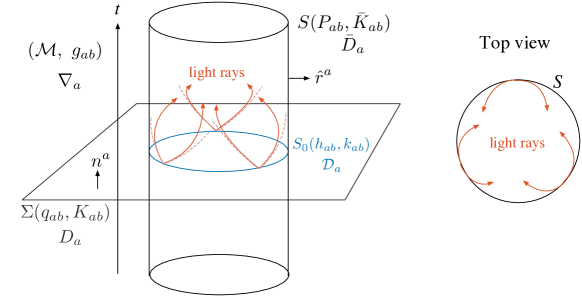
Figure 1: Schematic picture of the transversely trapping surface. The notations are also indicated.

Below, we derive the mathematical expression for the condition for $S$ to be a TTS. Before starting our analysis, we summarize the notations commonly used throughout this paper. The metric of the spacetime $\mathcal{M}$ is $g_{ab}$. With the future-directed unit normal $n^{a}$ to $\Sigma$, the induced metric and the extrinsic curvature of $\Sigma$ are given by $q_{ab}=g_{ab}+n_{a}n_{b}$ and $K_{ab}=(1/2)\pounds_{n}q_{ab}$, respectively, where $\pounds$ denotes the Lie derivative. With the outward unit normal $\hat{r}^{a}$ to $S$, the induced metric and the extrinsic curvature of $S$ are $P_{ab}=g_{ab}-\hat{r}_{a}\hat{r}_{b}$ and $\bar{K}_{ab}=(1/2)\pounds_{\hat{r}}P_{ab}$, respectively. Although the unit normal to $S$ in $\mathcal{M}$ and the unit normal to $S_{0}$ in $\Sigma$ do not coincide in general, in this paper we consider setups such that these two unit normals agree. We will come back to this point in Sects. 3.1 and 4.1. In this situation, the induced metric of $S_{0}$ is $h_{ab}=g_{ab}+n_{a}n_{b}-\hat{r}_{a}\hat{r}_{b}$, and its extrinsic curvature in the hypersurface $\Sigma$ is $k_{ab}=(1/2){}^{(3)}\pounds_{\hat{r}}h_{ab}$, where ${}^{(3)}\pounds$ is the Lie derivative on the hypersurface $\Sigma$. The covariant derivatives of $\mathcal{M}$, $\Sigma$, $S$, and $S_{0}$ are denoted as $\nabla_{a}$, $D_{a}$, $\bar{D}_{a}$, and $\mathcal{D}_{a}$, respectively. These definitions are summarized in Fig. 1.

Consider a null geodesic $\gamma$ with the tangent vector $k^{a}$ emitted tangentially to $S$ from a point $p$ on $S$. If $S$ is a TTS, this null geodesic must stay on $S$ or go toward the inside of $S$. Let us introduce another null trajectory $\bar{\gamma}$ from the point $p$ with the tangent vector $\bar{k}^{a}$, which is assumed to be a null geodesic on the hypersurface $S$,

$$\bar{k}^{a}\bar{D}_{a}\bar{k}^{c}=0.$$ (3)

At the point $p$, we choose $\bar{k}^{a}$ to be same as $k^{a}$, i.e. $k^{a}=\bar{k}^{a}$. Rewriting Eq. (3) in terms of the four-dimensional quantities, we have

$$a^{c}=-(\bar{K}_{ab}\bar{k}^{a}\bar{k}^{b})\hat{r}^{c},$$ (4)

where $a^{c}$ is four-acceleration, $a^{c}:=\bar{k}^{a}\nabla_{a}\bar{k}^{c}$. The two trajectories $\gamma$ and $\bar{\gamma}$ agree locally when $\bar{K}_{ab}\bar{k}^{a}\bar{k}^{b}=0$, and the four-acceleration $\bar{a}^{c}$ of $\bar{\gamma}$ is directed toward the outside if and only if $\bar{K}_{ab}\bar{k}^{a}\bar{k}^{b}<0$. This means that a four-dimensional null geodesic $\gamma$ satisfies the desired property if and only if $\bar{K}_{ab}k^{a}k^{b}\leq 0$ holds. This result is summarized as follows:

Proposition 1.

The necessary and sufficient condition for $S$ to be a TTS is that for every point on $S$, the condition

$$\bar{K}_{ab}k^{a}k^{b}\leq 0$$ (5)

holds for an arbitrary null tangent vector $k^{a}$ of $S$.

Hereafter, we call this condition the TTS condition. In Sects. 3.1 and 4.1, we will rewrite the TTS condition in the cases of static spacetimes and axisymmetric stationary spacetimes. Note that if the equality in (5) holds at all points on $S$, the surface $S$ coincides with the photon surface proposed in Claudel:2000 . Therefore, our definition of the TTS includes the photon surface as the marginal case.

In addition to the TTS condition, we sometimes require the two-surface $S_{0}$ to be a convex surface. The condition for the convexity depends on the choice of the slice $t=\mathrm{const}.$ We will specify this point in Sects. 3.1 and 4.1. When the convex condition is additionally imposed on the TTS, we call it the convex TTS.

2.2 Loosely trapped surfaces

Now, we explain the LTS defined in our previous paper Shiromizu:2017 . Consider the initial data $\Sigma$ of a (not necessarily static or stationary) spacetime $\mathcal{M}$ and a closed two-surface $S_{0}$ that divides $\Sigma$ into outside and inside regions. The initial data $\Sigma$ is supposed to have a nonnegative Ricci scalar ${}^{(3)}R\geq 0$. We introduce a radial foliation of $\Sigma$ starting from $S_{0}$ specified by the coordinate $r$ with the dual basis $D_{a}r=\hat{r}_{a}/\varphi$, where $\hat{r}_{a}$ is the unit normal to $S_{0}$ and $\varphi$ is the (spatial) lapse function. In this setup, the LTS is defined as follows:

Definition 2.

The surface $S_{0}$ is a loosely trapped surface if $k>0$ and $\hat{r}^{a}D_{a}k\geq 0$, where $k$ is the trace of the extrinsic curvature $k_{ab}$.

The motivation for this definition is that in the static slice of the Schwarzschild spacetime, the $r=\mathrm{const.}$ surface has this property in the range $2M<r\leq 3M$. Since $r=3M$ is the photon sphere, photons are loosely trapped inside of this sphere and the positivity of $\hat{r}^{a}D_{a}k$ is expected to be a useful indicator for a strong gravity region. Note that, as seen from the following formula which is derived from the trace of the Ricci equation with the double trace of the Gauss equation,

$$\hat{r}^{a}D_{a}k=-\frac{1}{2}\left({}^{(3)}R-{}^{(2)}R+k^{2}+k_{ab}k^{ab}\right)-\frac{1}{\varphi}\mathcal{D}^{2}\varphi,$$ (6)

the value of $\hat{r}^{a}D_{a}k$ depends on the choice of the lapse function $\varphi$. The surface $S_{0}$ is called an LTS if $\hat{r}^{a}D_{a}k\geq 0$ is satisfied (at least) for one choice of $\varphi$.

There are two main results in our previous paper Shiromizu:2017 . The first is that the LTS has topology $S^{2}$ and satisfies

$$\int_{S_{0}}k^{2}dA\leq\frac{16}{3}\pi.$$ (7)

This is proved by integrating the relation (6) under the condition $\hat{r}^{a}D_{a}k\geq 0$ and ${}^{(3)}R\geq 0$ and using the Gauss–Bonnet theorem. The second result is very important in this paper, and we state it in the form of a theorem:

Theorem 1.

If the inequality (7) is satisfied on $S_{0}$ with $k\geq 0$ in asymptotically flat initial data $\Sigma$ with nonnegative Ricci scalar ${}^{(3)}R$, the area $A_{0}$ of the surface $S_{0}$ satisfies the Penrose-like inequality (2), $A_{0}\leq 4\pi(3GM)^{2}$.

In order to prove this, we used the method of the inverse mean curvature flow originally proposed in Geroch:1973 ; Wald:1977 . The inverse mean curvature flow is generated by the lapse function $\varphi=1/k$, and along this flow, Geroch’s quasilocal energy is monotonic and asymptotes to the ADM mass at spacelike infinity $r\to\infty$. This leads to the bound on the surface area (see also Huisken:2001 for resolution of the possible formation of singularities along the flow). We refer to our previous paper Shiromizu:2017 for the detailed proof. Note that the theorem in Shiromizu:2017 states that the Penrose-like inequality holds for an LTS. We modified the statement of the theorem to the above because the inequality (7) and $k\geq 0$ on $S_{0}$ are necessary in the proof, but the LTS condition $\hat{r}^{a}D_{a}k\geq 0$ is not used directly; it was used to guarantee (7) in our previous paper. This modification will become important in Sects. 3.3 and 4.4.

3 Static spacetimes

In this section, we explore the properties of TTSs in static spacetimes. In Sect. 3.1, we explain the setup and rewrite the TTS condition. In Sect. 3.2, the relation between the TTS and the LTS is examined using the Einstein equations. The Penrose-like inequality for TTSs is proved in Sect. 3.3.

3.1 Setup and TTS condition

A static spacetime has the property that the timelike Killing vector field $t^{a}$ is hypersurface orthogonal Wald . Namely, there exist $t=\mathrm{const.}$ slices on which

$$t^{a}=\alpha n^{a}$$ (8)

holds (called static slices). Here, $\alpha$ is the lapse function. On this slice, the extrinsic curvature vanishes, $K_{ab}=0$. We will rewrite the TTS condition (5) using this slice. For this reason, our results below cannot be applied to the $t=\mathrm{const.}$ slice with nonvanishing $K_{ab}$. An example of static slices in a Schwarzschild spacetime is the $t=\mathrm{const.}$ hypersurfaces in the standard Schwarzschild coordinates $(t,r,\theta,\phi)$, and a counter-example is those of the Gullstrand–Painlevé coordinates Gullstrand:1922 .

For a static slice $\Sigma$, the unit normal to $S$ in $\mathcal{M}$ and that to $S_{0}$ in $\Sigma$ agree, and we denote those common normals as $\hat{r}^{a}$. It is easily derived that

$$\bar{K}_{ab}=-n_{a}n_{b}\frac{\hat{r}^{c}D_{c}\alpha}{\alpha}+k_{ab}$$ (9)

holds. Since the null tangent vector of $S$ is expressed as $k^{a}=n^{a}+s^{a}$, where $s^{a}$ is a unit tangent vector of $S_{0}$, the TTS condition (5) is rewritten as

$$k_{ab}s^{a}s^{b}\leq\frac{\hat{r}^{c}D_{c}\alpha}{\alpha}$$ (10)

for an arbitrary unit tangent vector $s^{a}$ of $S_{0}$. If we introduce a tensor

$$\sigma_{ab}:=k_{ab}-\frac{\hat{r}^{c}D_{c}\alpha}{\alpha}h_{ab},$$ (11)

the TTS condition (10) is equivalent to $\sigma_{ab}$ having two nonpositive eigenvalues. Such conditions are given by

$$\mathrm{tr}(\sigma_{ab})\leq 0\qquad\textrm{and}\qquad\mathrm{det}(\sigma_{ab})\geq 0.$$ (12)

After calculation, these two conditions can be expressed in a unified form,

$$\frac{k}{2}+\sqrt{\frac{1}{2}\tilde{k}_{ab}\tilde{k}^{ab}}\leq\frac{\hat{r}^{c}D_{c}\alpha}{\alpha},$$ (13)

where $k$ is the trace of $k_{ab}$ and $\tilde{k}_{ab}$ is the trace-free part of $k_{ab}$, i.e. $\tilde{k}_{ab}:=k_{ab}-(k/2)h_{ab}$. This is the TTS condition in the static case. Note that the condition (13) in the static case can be also derived by studying the geodesic equations directly. This is demonstrated in Appendix A.1.

For practical purposes, the following form may be more useful. Since $k_{ab}$ is a symmetric tensor, it can be diagonalized by appropriately choosing the tetrad basis $(\mathbf{e}^{1})_{a}$ and $(\mathbf{e}^{2})_{a}$ as

$$k_{ab}=k_{1}(\mathbf{e}^{1})_{a}(\mathbf{e}^{1})_{b}+k_{2}(\mathbf{e}^{2})_{a}(\mathbf{e}^{2})_{b}.$$ (14)

Without loss of generality, we can assume $k_{1}\geq k_{2}$. Using this form of $k_{ab}$, the TTS condition becomes

$$k_{1}\leq\frac{\hat{r}^{a}D_{a}\alpha}{\alpha}.$$ (15)

As defined in Sect. 2.1, we call $S$ a convex TTS when $S_{0}$ is a convex surface. The surface $S_{0}$ is a convex surface if and only if both $k_{1}$ and $k_{2}$ are nonnegative. Therefore, for $S$ to be a convex TTS, we require $k_{2}\geq 0$ in addition to the condition (15). The convex condition can also be expressed in a covariant manner as $k\geq\sqrt{2\tilde{k}_{ab}\tilde{k}^{ab}}$.

3.2 Connection to the LTSs

Below, we study the relation between convex TTSs and the LTSs. Specifically, the condition that a convex TTS becomes an LTS simultaneously is investigated using the Einstein equations. The projected components of the energy-momentum tensor $T_{ab}$ are defined as

$$\rho:=T_{ab}n^{a}n^{b},\qquad J_{a}:=-T_{bc}n^{b}{q^{c}}_{a},\qquad S_{ab}:=T_{cd}{q^{c}}_{a}{q^{d}}_{b}.$$ (16)

We adopt the $3+1$ split form of the Einstein equations. For a static spacetime,

$${}^{(3)}R = 16\pi G\rho,$$ (17a)

$${}^{(3)}R_{ab} = \frac{1}{\alpha}D_{a}D_{b}\alpha+8\pi G\left[S_{ab}+\frac{1}{2}q_{ab}(\rho-{S^{c}}_{c})\right].$$ (17b)

Here, Eq. (17a) is the Hamiltonian constraint, and Eq. (17b) is the evolution equation with $\pounds_{t}K_{ab}=0$. The momentum constraint is trivially satisfied with $J_{a}=0$. Taking the trace of Eq. (17b), we have

$$\frac{1}{\alpha}D^{2}\alpha=4\pi G\left(\rho+{S^{c}}_{c}\right).$$ (18)

Consider a convex TTS whose spatial section is $S_{0}$. The quantity $\hat{r}^{a}D_{a}k$ for $S_{0}$ is given by the formula (6). The three-dimensional Ricci scalar ${}^{(3)}R$ appearing in this equation can be expressed by the Gauss equation for $S_{0}$,

$${}^{(3)}R=2{}^{(3)}R_{ab}\hat{r}^{a}\hat{r}^{b}+{}^{(2)}R-k^{2}+k_{ab}k^{ab}.$$ (19)

The first term on the right-hand side of Eq. (19) can be written as

$${}^{(3)}R_{ab}\hat{r}^{a}\hat{r}^{b}=8\pi G(\rho+P_{r})-\frac{1}{\alpha}\mathcal{D}^{2}\alpha-k\frac{\hat{r}^{c}D_{c}\alpha}{\alpha},$$ (20)

which is obtained by multiplying Eq. (17b) by $\hat{r}^{a}\hat{r}^{b}$ and rewriting with Eq. (18). Here, we introduced pressure in the radial direction,

$$P_{r}:=T_{ab}\hat{r}^{a}\hat{r}^{b}.$$ (21)

As a result, the formula (6) is transformed into (see also Appendix C)

$$\hat{r}^{a}D_{a}k=-8\pi G(\rho+P_{r})+\frac{1}{\alpha}\mathcal{D}^{2}\alpha+k\frac{\hat{r}^{c}D_{c}\alpha}{\alpha}-k_{ab}k^{ab}-\frac{1}{\varphi}\mathcal{D}^{2}\varphi.$$ (22)

For this formula, we consider the condition that $S_{0}$ is guaranteed to satisfy the LTS condition $\hat{r}^{a}D_{a}k\geq 0$. Because the lapse function $\varphi$ can be freely chosen, we impose $\varphi=\alpha$ (if one considers the Schwarzschild spacetime, this corresponds to adopting the tortoise coordinate for $r$). The null energy condition indicates $\rho+P_{r}\geq 0$ in general, and hence we restrict to the situation $\rho+P_{r}=0$ on $S_{0}$. Using the expression (14) for $k_{ab}$ and applying the TTS condition (15) with the convex condition $k_{2}\geq 0$, we have

$$k\frac{\hat{r}^{c}D_{c}\alpha}{\alpha}-k_{ab}k^{ab}\geq k_{2}(k_{1}-k_{2})\geq 0.$$ (23)

Therefore, we have found the following:

Proposition 2.

A convex TTS $S$ in a static spacetime is an LTS as well if $\rho+P_{r}=0$ on $S$.

Note that the condition $\rho+P_{r}=0$ is not too strong because it must be imposed just on $S$ and it is satisfied if the region around $S$ is vacuum. Also, the Reissner–Nordström spacetimes satisfy this condition for $r=\mathrm{const.}$ surfaces. In this sense, we have proved the close connection between the TTS and the LTS with sufficient generality.

3.3 Area bound for TTSs

Once a TTS is proved to be an LTS, it possesses the properties that have been proved for LTSs. In particular, its area satisfies the Penrose-like inequality (2), $A_{0}\leq 4\pi(3GM)^{2}$. However, there might be the case that a TTS is not guaranteed to be an LTS but satisfies the Penrose-like inequality (i.e., we suppose that $\rho+P_{r}=0$ may not be necessary on $S$). Therefore, there remains a possibility that the condition can be relaxed if just the area bound is considered. Let us explore this possibility.

The strategy here is to find the condition that a convex TTS $S$ satisfies the inequality (7) without using the concept of the LTS, because the Penrose-like inequality follows from (7) by Theorem 1 in Sect. 2.2. Eliminating ${}^{(3)}R$ and $\hat{r}^{a}\hat{r}^{b}R_{ab}$ from Eqs. (17a), (19), and (20), we have (see also Appendix C)

$${}^{(2)}R=-16\pi GP_{r}+\frac{2}{\alpha}{\mathcal{D}^{2}\alpha}+2k\frac{\hat{r}^{a}D_{a}\alpha}{\alpha}+k^{2}-k_{ab}k^{ab}.$$ (24)

Using the expression (14) for $k_{ab}$ and the TTS condition (15), we have

$$2k\frac{\hat{r}^{a}D_{a}\alpha}{\alpha}+k^{2}-k_{ab}k^{ab}\geq\frac{3}{2}k^{2}+\frac{1}{2}(k_{1}+3k_{2})(k_{1}-k_{2})\geq\frac{3}{2}k^{2},$$ (25)

for a convex TTS. Assuming $P_{r}\leq 0$ and integrating the relation (24) over $S_{0}$, we have

$$\int_{S_{0}}{}^{(2)}RdA\geq\int_{S_{0}}\left(\frac{3}{2}k^{2}+\frac{2\mathcal{D}_{a}\alpha\mathcal{D}^{a}\alpha}{\alpha^{2}}\right)dA.$$ (26)

If $k>0$ at least at one point, the Gauss–Bonnet theorem tells us that $S_{0}$ has topology $S^{2}$ and the left-hand side is $\int{}^{(2)}RdA=8\pi$. This implies the inequality (7). Therefore, we have found the following:

Theorem 2.

The static time cross section of a convex TTS, $S_{0}$, has topology $S^{2}$ and satisfies the Penrose-like inequality $A_{0}\leq 4\pi(3GM)^{2}$ if $P_{r}\leq 0$ holds on $S_{0}$, $k>0$ at least at one point on $S_{0}$, and ${}^{(3)}R$ is nonnegative (i.e. the energy density $\rho\geq 0$) in the outside region on a static slice in an asymptotically flat static spacetime.

Compared to Proposition 2 in Sect. 3.2, the equality $\rho+P_{r}=0$ is relaxed to the inequality $P_{r}\leq 0$. Therefore, Theorem 2 is expected to have greater applicability. Note that from Eq. (25), this theorem also holds for a nonconvex TTS if $k_{2}$ is within the range $k_{2}\geq-k_{1}/3$.

4 Axisymmetric stationary spacetimes

In this section, we explore the properties of axisymmetric TTSs in (nonstatic) stationary spacetimes with axial symmetry. In Sect. 4.1, we explain the setup in detail and rewrite the TTS condition. In Sect. 4.2, we show that TTSs actually can exist in a stationary spacetime by presenting examples of a Kerr spacetime. In Sect. 4.3, the relation between the TTS and the LTS is examined, but for fairly restricted situations. The Penrose-like inequality for the TTS is proved in Sect. 4.4.

4.1 Setup and TTS condition

Consider an axisymmetric stationary spacetime $\mathcal{M}$. There are two Killing vector fields: One is the timelike Killing vector field $t^{a}$ and the other is a spacelike Killing vector field $\phi^{a}$ that represents $U(1)$ isometry. Since these two Killing fields have been proved to commute Carter:1970 , it is possible to adopt a $t=\mathrm{const.}$ slice on which $U(1)$ symmetry becomes manifest. In addition, we require the existence of two-dimensional surfaces that are orthogonal to both $t^{a}$ and $\phi^{a}$ (called the $t$–$\phi$ orthogonality property). The necessary and sufficient condition for this requirement is proved to be Carter:1969

$$t^{a}T_{a[b}t_{c}\phi_{d]}\ =\ \phi^{a}T_{a{[}b}t_{c}\phi_{d]}\ =\ 0.$$ (27)

Physically, this condition means that matter, if it exists, is moving just in the $\phi^{a}$ direction. In this case, there exists the symmetry of the metric under the transformation $t^{a}\to-t^{a}$ and $\phi^{a}\to-\phi^{a}$.

Since we consider the nonstatic case in this section, the timelike Killing field is decomposed as

$$t^{a}=\alpha n^{a}+\beta^{a},$$ (28)

where $\alpha$ is the lapse function and $\beta^{a}$ is the shift vector. Here, we consider the time slice on which the shift vector $\beta^{a}$ is proportional to the Killing vector field $\phi^{a}$,

$$\beta^{a}=-\omega\phi^{a}.$$ (29)

Here, the quantity $\omega$ in Eq. (29) corresponds to the angular velocity of the zero-angular-momentum observers (ZAMOs). Note that this condition is realized only on a special slice. For example, although the Boyer–Lindquist coordinates of the Kerr spacetime possess this property, other coordinates like the Kerr–Schild coordinates Kerr:1963 or the Doran coordinates Doran:1999 do not satisfy this condition because the shift vector has a radial component.

In this paper, we consider only axisymmetric TTSs for a technical reason. If a TTS $S$ is axisymmetric, the timelike unit normal $n^{a}$ to $\Sigma$ becomes a tangent vector of $S$, because both $t^{a}$ and $\beta^{a}$ are tangent to $S$. Then, the outward unit normal $\hat{r}^{a}$ to $S$ becomes the outward unit normal to $S_{0}$ in $\Sigma$ as well. If $S$ is not axisymmetric, these properties do not hold and the analysis becomes complicated. The study of nonaxisymmetric TTSs in the stationary case is left as a remaining problem.

Let us start the derivation of the TTS condition in the axisymmetric stationary spacetime. Because the induced metric of $S$ is given by $P_{ab}=-n_{a}n_{b}+h_{ab}$ in this setup, we have

$$\bar{K}_{ab}=\frac{1}{2}\pounds_{\hat{r}}P_{ab}=-n_{a}n_{b}\frac{\hat{r}^{c}D_{c}\alpha}{\alpha}+\frac{1}{2}\pounds_{\hat{r}}h_{ab}.$$ (30)

On the other hand, rewriting the three-dimensional quantities by the four-dimensional quantities, we have

$$k_{ab}=\frac{1}{2}{}^{(3)}\pounds_{\hat{r}}h_{ab}=\frac{1}{2}\pounds_{\hat{r}}h_{ab}+\frac{1}{2}(n^{d}\nabla_{d}\hat{r}^{c}-\hat{r}^{d}\nabla_{d}n^{c})(n_{a}h_{cb}+n_{b}h_{ca}).$$ (31)

Putting these together, the decomposition of the extrinsic curvature of $S$ is given as

$$\bar{K}_{ab}\ =\ -n_{a}n_{b}\frac{\hat{r}^{c}D_{c}\alpha}{\alpha}+k_{ab}-n_{a}v_{b}-n_{b}v_{a}.$$ (32)

with

$$v_{a}=\frac{1}{2}h_{ab}\pounds_{n}\hat{r}^{b}.$$ (33)

Note that $v_{a}$ can be regarded as the cross-components of $\bar{K}_{ab}$, that is, $v_{a}={h_{a}}^{b}\bar{K}_{bc}n^{c}$. Now, we recall the TTS condition (5). As in the static case, the null tangent vector of $S$ is decomposed as $k^{a}=n^{a}+s^{a}$ with a unit tangent vector $s^{a}$ of $S_{0}$. Then, the TTS condition in this case is that

$$k_{ab}s^{a}s^{b}+2v_{b}s^{b}\leq\frac{\hat{r}^{c}D_{c}\alpha}{\alpha}$$ (34)

holds for an arbitrary unit tangent vector $s^{a}$ of $S_{0}$.

This condition can be simplified further. Because $S$ is stationary and axisymmetric, the unit normal $\hat{r}^{a}$ of $S$ is Lie transported along the integral lines of the Killing vectors: $\pounds_{t}\hat{r}^{a}={}^{(3)}\pounds_{\phi}\hat{r}^{a}=0.$ Using this relation, the vector $v^{b}$ is rewritten as

$$v_{a}=\frac{1}{2\alpha}h_{ab}{}^{(3)}\pounds_{\hat{r}}\beta^{b}=-\frac{1}{2\alpha}(\hat{r}^{b}D_{b}\omega){\phi}_{a}.$$ (35)

On the other hand, the assumption of symmetry under the transformation $t^{a}\to-t^{a}$ and $\phi^{a}\to-\phi^{a}$ (the $t$–$\phi$ orthogonality property) implies that the geometry of the $t=\mathrm{const.}$ slice has symmetry under $\phi^{a}\to-\phi^{a}$. Therefore, the extrinsic curvature of $S_{0}$ satisfies $k_{ab}\hat{\theta}^{a}{\phi}^{b}=0$, where $\hat{\theta}^{a}$ is the unit tangent vector of $S_{0}$ orthogonal to ${\phi}^{a}$. Hence, introducing the tetrad basis as $(\mathbf{e}^{1})_{a}=\phi_{a}/\phi$ and $(\mathbf{e}^{2})_{a}=\hat{\theta}_{a}$ (with $\phi=\sqrt{\phi^{a}\phi_{a}}$), $k_{ab}$ and $v_{a}$ are expressed as

$$k_{ab} = k_{1}(\mathbf{e}^{1})_{a}(\mathbf{e}^{1})_{b}+k_{2}(\mathbf{e}^{2})_{a}(\mathbf{e}^{2})_{b},$$ (36a)

$$v_{a} = v_{1}(\mathbf{e}^{1})_{a},$$ (36b)

with $v_{1}=-({\phi}/{2\alpha})(\hat{r}^{b}D_{b}\omega)$. Setting $s_{a}=\cos\xi(\mathbf{e}^{1})_{a}+\sin\xi(\mathbf{e}^{2})_{a}$ and substituting these expressions into (34), the function

$$f(\cos\xi)=(k_{2}-k_{1})\cos^{2}\xi-2v_{1}\cos\xi+\frac{\hat{r}^{c}D_{c}\alpha}{\alpha}-k_{2}$$ (37)

must be nonnegative for arbitrary $0\leq\xi<2\pi$. This condition can be re-expressed in terms of the relation between the coefficients (see Appendix B for a derivation), and we have the following result:

Proposition 3.

The necessary and sufficient condition for $S$ to be an axisymmetric TTS in an axisymmetric stationary spacetime with the $t$–$\phi$ orthogonality property is that one of the following three conditions is satisfied at any point on $S_{0}$:

(i) $$\frac{\hat{r}^{c}D_{c}\alpha}{\alpha}-k_{1}\geq|2v_{1}|>2(k_{2}-k_{1})>0;$$ (38a)

(ii) $$\frac{\hat{r}^{c}D_{c}\alpha}{\alpha}-k_{2}\geq\frac{v_{1}^{2}}{k_{2}-k_{1}}\qquad\textrm{and}\qquad k_{2}-k_{1}\geq|v_{1}|;$$ (38b)

(iii) $$\frac{\hat{r}^{c}D_{c}\alpha}{\alpha}-|2v_{1}|\geq k_{1}\geq k_{2}.$$ (38c)

Similarly to the static case, this condition can be derived by directly studying the geodesic equations. This is demonstrated in Appendix A.2. For a convex TTS, the conditions $k_{1}\geq 0$ and $k_{2}\geq 0$ are additionally required.

4.2 Examples in a Kerr spacetime

Here, we explicitly demonstrate that TTSs exist in a stationary spacetime using the Kerr spacetime as an example. We start with a sufficiently general metric of axisymmetric stationary spacetimes possessing the $t$–$\phi$ orthogonality property,

$$ds^{2}=-{\alpha}^{2}dt^{2}+\gamma^{2}(d\phi-\omega dt)^{2}+\varphi^{2}dr^{2}+\psi^{2}d\theta^{2},$$ (39)

where all metric functions depend on $r$ and $\theta$ only. Here, $\alpha$ and $\omega$ are same as those given in Eqs. (28) and (29) (i.e., the lapse function and the ZAMO angular velocity). Here, we consider the condition that the surface $r=\mathrm{const.}$ becomes a TTS. The tetrad components of the extrinsic curvature $k_{ab}$ and the vector $v_{a}$ defined in Eqs. (36a) and (36b) are calculated as

$$k_{1}=\frac{\gamma_{,r}}{\varphi\gamma},\qquad k_{2}=\frac{\psi_{,r}}{\varphi\psi},\qquad v_{1}=-\frac{\gamma\omega_{,r}}{2\varphi\alpha},$$ (40)

and the relation $\hat{r}^{c}D_{c}\alpha/\alpha=\alpha_{,r}/(\varphi\alpha)$ is also used.

The metric functions of a Kerr spacetime in the Boyer–Lindquist coordinates (with $G=1$) are given by

$${\alpha}^{2}=\frac{\Delta\Sigma}{\mathcal{A}},\qquad\gamma^{2}=\frac{\mathcal{A}\sin^{2}\theta}{\Sigma},\qquad\omega=\frac{2Mar}{\mathcal{A}},\qquad\varphi^{2}=\frac{\Sigma}{\Delta},\qquad\psi^{2}=\Sigma,$$ (41)

with

$$\Sigma=r^{2}+a^{2}\cos^{2}\theta,\qquad\Delta=r^{2}+a^{2}-2Mr,$$ (42a)

$$\mathcal{A}=(r^{2}+a^{2})^{2}-\Delta a^{2}\sin^{2}\theta.$$ (42b)

Here, $M$ is the ADM mass and $a$ is the rotation parameter that is related to the ADM angular momentum as $J=Ma$. The event horizon is located at $r=r_{+}=M+\sqrt{M^{2}-a^{2}}$. We consider the parameter region $0<a\leq M$, i.e., a nonstatic spacetime with an event horizon.

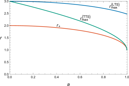
Figure 2: The behavior of $r^{\rm(TTS)}_{\rm max}$ and $r^{\rm(LTS)}_{\rm max}$ as functions of $a$. The unit of the length is $M$.

For a Kerr spacetime, it is easy to check $k_{2}>k_{1}$, which is natural because the Kerr black hole has oblate geometry. Although the calculation is more tedious, one can show that $v_{1}^{2}>(k_{2}-k_{1})^{2}$ holds. Therefore, we consider case (i) of Proposition 38, and the inequality ${\hat{r}^{c}D_{c}\alpha}/{\alpha}-k_{1}\geq|2v_{1}|$ in (38a) determines the range of $r$. The squared inequality gives the condition

$$r(r-3M)^{2}\geq 4a^{2}M$$ (43)

on the equatorial plane $\theta=\pi/2$ (the condition is weaker for other $\theta$ values). There are two domains satisfying this inequality, and just the inner one satisfies the nonsquared inequality (in the outer domain, ${\hat{r}^{c}D_{c}\alpha}/{\alpha}-k_{1}$ becomes negative). In this way, we find that the surface $r=\textrm{const.}$ is a TTS for

$$r_{+}<r<r^{\rm(TTS)}_{\rm max}=2M\left\{1+\cos\left[\frac{2}{3}\arccos\left(-\frac{a}{M}\right)\right]\right\}.$$ (44)

The behavior of $r^{\rm(TTS)}_{\rm max}$ is shown as a function of $a/M$ in Fig. 2. Note that the value of $r^{\rm(TTS)}_{\rm max}$ corresponds to the radius of the circular orbit of a photon closest to the black hole (e.g., p. 73 of Frolov:1998 ). Therefore, our result is reasonable because only photons propagating on the equatorial plane in the direction of the black hole rotation propagate on the surface $r=r^{\rm(TTS)}_{\rm max}$, and all other photons initially moving in the tangent direction to the surface will fall into the black hole.

Let us also look at LTSs in the Kerr spacetime. A surface $r=\mathrm{const.}$ becomes an LTS when $k_{,r}\geq 0$ is satisfied at every point. This condition becomes strictest on the equatorial plane $\theta=\pi/2$, and there exists a maximum radius $r^{\rm(LTS)}_{\rm max}$ such that an $r=\mathrm{const}.$ surface becomes an LTS for $r_{+}\leq r\leq r^{\rm(LTS)}_{\rm max}$. Unfortunately, no simple analytic formula for $r^{\rm(LTS)}_{\rm max}$ seems to exist, unlike the TTS case. The behavior of $r^{\rm(LTS)}_{\rm max}$ is shown in Fig. 2. Although $r^{\rm(LTS)}_{\rm max}=r^{\rm(TTS)}_{\rm max}=3M$ at $a/M=0$, LTSs distribute in a broader region compared to TTSs when $a/M$ is large. While $r=r^{\rm(TTS)}_{\rm max}$ indicates the inner edge of the photon region, $r=r^{\rm(LTS)}_{\rm max}$ is located in the middle of the photon region. In this sense, the TTS and the LTS are different indicators for strong gravity regions, and the TTS is a stricter one compared to the LTS.

4.3 Connection to the LTSs

Here, we try to derive the condition that a convex TTS becomes an LTS using the Einstein equation. Since $\pounds_{t}h_{ab}=0$ in a stationary spacetime, we have

$$K_{ab}=-\frac{1}{2\alpha}\left(D_{a}\beta_{b}+D_{b}\beta_{a}\right).$$ (45)

Using the projection (16) of the energy momentum tensor, the Einstein equations in the $3+1$ split form are

$${}^{(3)}R+K^{2}-K_{ab}K^{ab} = 16\pi G\rho,$$ (46a)

$$D_{a}{K^{a}}_{b}-D_{b}K = -8\pi GJ_{b},$$ (46b)

$${}^{(3)}R_{ab}+K_{ab}K-2K_{ac}{K^{c}}_{b} = \frac{1}{\alpha}{}^{(3)}\pounds_{\beta}K_{ab}+\frac{1}{\alpha}D_{a}D_{b}\alpha$$ (46c)

$$\qquad+8\pi G\left[S_{ab}+\frac{1}{2}q_{ab}(\rho-{S^{c}}_{c})\right].$$

Here, Eqs. (46a) and (46b) are the Hamiltonian and momentum constraints, respectively, and Eq. (46c) is the evolution equation with $\pounds_{t}K_{ab}=0$. Because of the axisymmetry of the space $\Sigma$, the Lie derivatives with respect to $\phi^{a}$ of the geometric quantities become zero:

$${}^{(3)}\pounds_{\phi}\alpha\ =\ {}^{(3)}\pounds_{\phi}\beta^{a}\ =\ {}^{(3)}\pounds_{\phi}q_{ab}\ =\ {}^{(3)}\pounds_{\phi}K_{ab}\ =\ 0.$$ (47)

Here, ${}^{(3)}\pounds_{\phi}q_{ab}=0$ is equivalent to the Killing equation of $\phi^{a}$ on $\Sigma$, $D_{a}\phi_{b}+D_{b}\phi_{a}=0$. From Eq. (29), ${}^{(3)}\pounds_{\phi}\beta^{a}=0$ is equivalent to $\phi^{b}D_{b}\omega=0$, and

$$K_{ab}=\frac{1}{2\alpha}\left(\phi_{a}D_{b}\omega+\phi_{b}D_{a}\omega\right).$$ (48)

Taking the trace of this relation, we have $K=0$, i.e. the spacelike hypersurface $\Sigma$ is maximally sliced. Substituting these relations, the Hamiltonian constraint (46a) and the evolution equation (46c) become

$${}^{(3)}R = \frac{\phi^{2}}{2\alpha^{2}}(D_{b}\omega D^{b}\omega)+16\pi G\rho,$$ (49a)

$${}^{(3)}R_{ab} = \frac{1}{2\alpha^{2}}\left[\phi_{a}\phi_{b}(D_{c}\omega D^{c}\omega)-\phi^{2}D_{a}\omega D_{b}\omega\right]$$ (49b)

$$\qquad\qquad\qquad+\frac{1}{\alpha}D_{a}D_{b}\alpha+8\pi G\left[S_{ab}+\frac{1}{2}q_{ab}(\rho-{S^{c}}_{c})\right],$$

with $\phi^{2}=\phi^{a}\phi_{a}$. The trace of Eq. (49b) gives

$$\frac{1}{\alpha}D^{2}\alpha=\frac{\phi^{2}}{2\alpha^{2}}(D_{c}\omega D^{c}\omega)+4\pi G(\rho+{S^{c}}_{c}).$$ (50)

Consider a convex TTS whose spatial section is $S_{0}$. We rewrite the formula (6) for $\hat{r}^{a}D_{a}k$ of $S_{0}$ using the Gauss equation (19). The quantity ${}^{(3)}R_{ab}\hat{r}^{a}\hat{r}^{b}$ in Eq. (19) is rewritten by

$${}^{(3)}R_{ab}\hat{r}^{a}\hat{r}^{b}=8\pi G(\rho+P_{r})-\frac{1}{\alpha}\mathcal{D}^{2}\alpha-k\frac{\hat{r}^{c}D_{c}\alpha}{\alpha}+\frac{\phi^{2}}{2\alpha^{2}}(\mathcal{D}_{c}\omega\mathcal{D}^{c}\omega),$$ (51)

which is obtained by multiplying Eq. (49b) by $\hat{r}^{a}\hat{r}^{b}$ and rewriting with Eq. (50). Here, $P_{r}$ is the pressure in the radial direction introduced in Eq. (21). The result is (see also Appendix C)

$$\hat{r}^{a}D_{a}k\ =\ -8\pi G(\rho+P_{r})+\frac{1}{\alpha}\mathcal{D}^{2}\alpha+k\frac{\hat{r}^{c}D_{c}\alpha}{\alpha}-k_{ab}k^{ab}-\frac{\phi^{2}}{2\alpha^{2}}(\mathcal{D}_{c}\omega\mathcal{D}^{c}\omega)-\frac{1}{\varphi}\mathcal{D}^{2}\varphi.$$ (52)

We would like to find the condition that the positivity of $\hat{r}^{a}D_{a}k$ is guaranteed. Similarly to the static case, we impose $\varphi=\alpha$ and $\rho+P_{r}=0$. Then, if the condition

$$k\frac{\hat{r}^{c}D_{c}\alpha}{\alpha}-k_{ab}k^{ab}\geq\frac{\phi^{2}}{2\alpha^{2}}(\mathcal{D}_{c}\omega\mathcal{D}^{c}\omega)$$ (53)

is satisfied, a TTS is guaranteed to be an LTS. However, unlike in the static case, the existence of the right-hand side makes it difficult to prove this inequality.

Figure 3: Contour surfaces of the ZAMO angular velocity $\omega$ for $\omega/\Omega_{\rm H}=n/10$ with $n=1,...,10$, where $\Omega_{\rm H}$ is the angular velocity of the event horizon, in the $(r\cos\theta,r\sin\theta)$-plane of a Kerr spacetime with $a/M=0.99$. The unit of the length is $M$.

Instead of making a general argument, we consider surfaces each of which is given by $\omega=\mathrm{const.}$ The $\omega=\mathrm{const.}$ surface consists of trajectories of ZAMO observers with the same angular velocity $\omega$. Examples of contour surfaces of the ZAMO angular velocity are depicted in Fig. 3 in the case of a Kerr spacetime with $a/M=0.99$. These surfaces are approximately the same as the $r=\mathrm{const.}$ surfaces. For this surface, the right-hand side of the inequality (53) vanishes. By setting $s^{a}=\pm(\mathbf{e}^{1})^{a}$ and $(\mathbf{e}^{2})^{a}$ in the TTS condition (34), we have ${\hat{r}^{c}D_{c}\alpha}/{\alpha}\geq k_{1}+2|v_{1}|\geq k_{1}$ and ${\hat{r}^{c}D_{c}\alpha}/{\alpha}\geq k_{2}$. These two inequalities are expressed as ${\hat{r}^{c}D_{c}\alpha}/{\alpha}\geq k_{\rm L}$ by setting $k_{\rm L}:=\mathrm{max}(k_{1},k_{2})$ and $k_{\rm S}:=\mathrm{min}(k_{1},k_{2})$. Using this, the relation

$$k\frac{\hat{r}^{c}D_{c}\alpha}{\alpha}-k_{ab}k^{ab}=k_{\rm S}(k_{\rm L}-k_{\rm S})\geq 0$$ (54)

holds for a convex TTS. To summarize, we have proved the following:

Proposition 4.

If a contour surface of the ZAMO angular velocity is a convex TTS and $\rho+P_{r}=0$ on it, it is an LTS as well.

Compared to the static case, the argument here is fairly restricted, not because a convex TTS is not an LTS in many situations, but because the method here does not work sufficiently. As we have seen in the Kerr case, the TTSs given by $r=\mathrm{const}.$ surfaces are simultaneously LTSs for all $0\leq a/M\leq 1$. We expect that a better method may establish the connection between the TTS and the LTS in the axisymmetric stationary case more firmly. This is left as a remaining problem.

4.4 Area bound for TTSs

If we are only interested in the area bound by the Penrose-like inequality, it is possible to relax the condition of Proposition 4 in a similar manner to the static case in Sect. 3.3. Namely, we consider the condition that leads to the inequality (7) on a convex TTS $S$ without using the concept of the LTS. Eliminating ${}^{(3)}R$ and ${}^{(3)}R_{ab}\hat{r}^{a}\hat{r}^{b}$ from Eqs. (19), (49a), and (51), we have (see also Appendix C)

$${}^{(2)}R=-16\pi GP_{r}+\frac{2}{\alpha}{\mathcal{D}^{2}\alpha}+2k\frac{\hat{r}^{a}D_{a}\alpha}{\alpha}+k^{2}-k_{ab}k^{ab}+\frac{\phi^{2}}{2\alpha^{2}}\left[(\hat{r}^{a}D_{a}\omega)^{2}-(\mathcal{D}_{a}\omega\mathcal{D}^{a}\omega)\right].$$ (55)

The inequality ${\hat{r}^{c}D_{c}\alpha}/{\alpha}\geq k_{\rm L}$ implies

$$2k\frac{\hat{r}^{a}D_{a}\alpha}{\alpha}+k^{2}-k_{ab}k^{ab}\geq\frac{3}{2}k^{2}+\frac{1}{2}(k_{\rm L}+3k_{\rm S})(k_{\rm L}-k_{\rm S})\geq\frac{3}{2}k^{2}$$ (56)

for a convex TTS (a nonconvex TTS also satisfies this inequality if $k_{\rm S}$ is within the range $k_{\rm S}\geq-k_{\rm L}/3$). Assuming $P_{r}\leq 0$ and integrating the relation (55), we have

$$\int_{S_{0}}{}^{(2)}RdA\geq\int_{S_{0}}\left\{\frac{3}{2}k^{2}+\frac{2\mathcal{D}_{a}\alpha\mathcal{D}^{a}\alpha}{\alpha^{2}}+\frac{\phi^{2}}{2\alpha^{2}}\left[(\hat{r}^{a}D_{a}\omega)^{2}-(\mathcal{D}_{a}\omega\mathcal{D}^{a}\omega)\right]\right\}dA.$$ (57)

If the right-hand side is positive, $S_{0}$ has topology $S^{2}$ and the left-hand side becomes $\int_{S_{0}}{}^{(2)}RdA=8\pi$ because of the Gauss–Bonnet theorem. Therefore, we have the following result:

Theorem 3.

The time cross section of an axisymmetric convex TTS, $S_{0}$, has topology $S^{2}$ and satisfies the Penrose-like inequality $A_{0}\leq 4\pi(3GM)^{2}$ if $P_{r}\leq 0$ and

$$\frac{4}{\phi^{2}}(\mathcal{D}_{a}\alpha\mathcal{D}^{a}\alpha)+(\hat{r}^{a}D_{a}\omega)^{2}\geq(\mathcal{D}_{a}\omega\mathcal{D}^{a}\omega)$$ (58)

holds on $S_{0}$, $k>0$ at least at one point on $S_{0}$, and ${}^{(3)}R$ is nonnegative in the outside region in an asymptotically flat axisymmetric stationary spacetime with the $t$–$\phi$ orthogonality property.

Here, we discuss to what extent the condition (58) is strong. Since $\phi^{a}\mathcal{D}_{a}\omega=0$, the right-hand side is rewritten as $(\hat{\theta}^{a}D_{a}\omega)^{2}$. This quantity is zero at the symmetry axis, and also on an equatorial plane (if it exists). Therefore, the condition (58) is satisfied at least at these two locations. Furthermore, since the ZAMO angular momentum $\omega$ coincides with the (constant) horizon angular velocity $\Omega_{\rm H}$ on the event horizon, the condition (58) must be satisfied at least on surfaces sufficiently close to the event horizon. For this reason, the condition (58) does not restrict the situation strongly, and hence many TTSs satisfying this condition should exist. In fact, we can check that this condition is satisfied by arbitrary $r=\mathrm{const.}$ surfaces of a Kerr spacetime. Therefore, Theorem 3 is expected to have sufficient generality.

5 Summary and discussion

In this paper, we have defined a new concept, the transversely trapping surface, as a generalization of static photon surfaces. Its definition was introduced in Sect. 2.1 (Definition 1), and the condition for a surface $S$ to be a TTS is mathematically expressed as Eq. (5) in Proposition 1. The properties of the TTS in static spacetimes were studied in Sect. 3. There, a TTS is proved to be a loosely trapped surface as defined in our previous paper Shiromizu:2017 (see Definition 2 of this paper) at the same time under certain conditions (Proposition 2 in Sect. 3.2). The area of a TTS is shown to satisfy the Penrose-like inequality (2) under some generic conditions (Theorem 2 in Sect. 3.3).

In Sect. 4, we studied TTSs in axisymmetric stationary spacetimes. Because of a technical reason, we considered axisymmetric TTSs in spacetimes with the $t$–$\phi$ orthogonality property. The TTS condition in this setup was summarized in a concise form (Proposition 38 in Sect. 4.1). It was explicitly shown that TTSs exist in a Kerr spacetime (Sect. 4.2). As for the connection to the LTS, we have shown that TTSs given by contour surfaces of the ZAMO angular velocity are LTSs at the same time under certain conditions (Proposition 4 in Sect. 4.3). This fairly restricted argument is due to a technical reason, and generalization is left as an open problem. However, we have proved the Penrose-like inequality (2) under fairly general situations (Theorem 3 in Sect. 4.4).

We have established that the area of a TTS is bounded from above by the area of a photon sphere with the same mass in quite generic static/stationary situations. This is a natural result, because if photons propagating in the transverse direction to the source are trapped, such a region must be compact so that gravity is sufficiently strong.

It is interesting to list spacetimes possessing TTSs. Black hole spacetimes generally possess TTSs around their horizons. In addition to the vacuum black holes, black holes surrounded by ring-shaped matter Ansorg:2005 and those with scalar or proca hairs Herdeiro:2014 ; Herdeiro:2015 ; Herdeiro:2016 also possess TTSs. There are a few examples of spacetimes without horizons where TTSs are present. One is a spherically symmetric star composed of incompressible fluid (e.g., Wald ): the radius of such a star $R$ can be as small as $8/3\leq R/M\leq 3$ without violating the dominant energy condition. Another example is the soliton-like structure of a complex massive scalar field, the so-called boson star. It has been reported in Horvat:2013 that a boson star can have a photon sphere (and, therefore, TTSs), although the binding energy is not negative for such situations if the scalar field is minimally coupled to gravity. Other rather exotic examples are spacetimes with naked singularities, as studied in Virbhadra:2002 ; Bozza:2002 ; Virbhadra:2007 ; Sahu:2012 ; Sahu:2013 .

In this paper, we restricted the definition of the TTS as a static/stationary surface in a static/stationary spacetime. It would be possible to generalize this definition to more general surfaces in dynamical spactimes. For example, one may define the generalized TTS as an arbitrary spatially bounded timelike surface $S$ on which the TTS condition $\bar{K}_{ab}k^{a}k^{b}\leq 0$ holds for arbitrary null tangent vectors $k^{a}$ everywhere. Taking account of this possibility, in Appendix C we present some useful geometric formulas in the setup given by Fig. 1 but without assuming the timelike Killing symmetry. As special cases, the formulas in the main text are rederived as a consistency check.

There are many possible directions of extensions of our current work. Some examples are listed here. First, for axisymmetric spacetimes with nonvanishing global angular momentum $J$, a generalization of the Penrose inequality ,

$$A_{\rm H}\leq 8\pi G^{2}\left(M^{2}+\sqrt{M^{4}-\frac{J^{2}}{G^{2}}}\right),$$ (59)

has been conjectured for apparent horizons Dain:2002 . Namely, the bound of the apparent horizon area is expected to become stronger as $J$ is increased. From the study of a Kerr spacetime in Sect. 4.2 of this paper, the same tendency is also expected for TTSs. Looking for a stronger bound of the TTS area depending on $J$ is an interesting problem. Furthermore, an inequality of a different type,

$$8\pi G|J_{q}|\leq A_{\rm H},$$ (60)

has been proved for an apparent horizon in an axisymmetric spacetime under some generic conditions, where $J_{q}$ is an appropriately defined quasilocal angular momentum Dain:2011 . The lower bound of the TTS area in terms of $J_{q}$ is also an interesting issue.

Second, there is another formulation for compactness of an apparent horizon, the hoop conjecture Thorne:1972 , which states that black holes with horizons form when and only when a mass $M$ gets compacted into a region whose circumference in every direction is bounded by $C\lesssim 2\pi(2GM)$. The important claim of this conjecture is that an apparent horizon does not become arbitrarily long in one direction, and this property was shown to hold in several examples (e.g., Yoshino:2007 ). It would be interesting to test whether TTSs also satisfy this property. We expect that an argument such that the circumference of a TTS is bounded as $C\lesssim 2\pi(3GM)$ could be made.

Finally, since a TTS suggests that gravity is strong there, ordinary matter would not be able to support itself inside of the TTS. Therefore, it would be possible to show the existence of a horizon inside of a TTS under some conditions. In the spherically symmetric case, it has been shown that a perfect fluid star consisting of polytropic balls cannot possess a photon sphere Saida:2015 . We expect that it would be possible to generalize such an argument for nonspherical TTSs applying the methods for proving singularity theorems.

The work of H. Y. was in part supported by a Grant-in-Aid for Scientific Research (A) (No. 26247042) from the Japan Society for the Promotion of Science (JSPS). K. I. is supported by a JSPS Grant-in-Aid for Young Scientists (B) (No. 17K14281). T. S. is supported by a Grant-in-Aid for Scientific Research (C) (No. 16K05344) from JSPS.

Appendix A TTS conditions from geodesic equations

The purpose of this appendix is to demonstrate that the TTS conditions in the static case and in the axisymmetric stationary case can be derived by directly examining the geodesic equations.

A.1 Static spacetimes

The metric of a static spacetime with static slices $t=\mathrm{const.}$ is given by

$$ds^{2}=-\alpha^{2}dt^{2}+\varphi^{2}dr^{2}+h_{IJ}dx^{I}dx^{J}.$$ (61)

Consider a null geodesic whose tangent vector is $k^{a}=(\dot{t},\dot{r},\dot{x}^{I})$ with $I=1$ and $2$, where the dot denotes the derivative with respect to the affine parameter. For a surface $S$ given by $r=\mathrm{const.}$ to be a TTS, $\ddot{r}\leq 0$ must hold for arbitrary $k^{a}$ with $\dot{r}=0$ at arbitrary points on $S$. The radial equation is given by

$$\ddot{r}=-\frac{\alpha\alpha_{,r}}{\varphi^{2}}\dot{t}^{2}-\frac{\varphi_{,r}}{\varphi}\dot{r}^{2}-\frac{2\varphi_{,I}}{\varphi}\dot{x}^{I}\dot{r}+\frac{h_{IJ,r}}{2\varphi^{2}}\dot{x}^{I}\dot{x}^{J}.$$ (62)

Imposing $\dot{r}=0$ and eliminating $\dot{t}$ using the null condition $k_{a}k^{a}=0$, we have

$$\ddot{r}=\frac{1}{\varphi}\left(k_{IJ}-\frac{\hat{r}^{a}D_{a}\alpha}{\alpha}h_{IJ}\right)\dot{x}^{I}\dot{x}^{J},$$ (63)

where we used $\hat{r}^{a}D_{a}\alpha=\alpha_{,r}/\varphi$ and $k_{IJ}=h_{IJ,r}/{2\varphi}$. In order that $\ddot{r}\leq 0$ holds for arbitrary $\dot{x}^{I}$, the matrix $\sigma_{ab}$ defined in (11) must have two nonpositive eigenvalues. Therefore, we obtain the same TTS condition.

A.2 Axisymmetric stationary spacetimes

We study the geodesic equation of an axisymmetric stationary spacetime with the $t$–$\phi$ orthogonality property using the general metric (39). Similarly to the static case, we consider a null geodesic with a tangent vector $k^{a}=(\dot{t},\dot{r},\dot{\theta},\dot{\phi})$, and require a surface $S$ given by $r=\mathrm{const.}$ to be a TTS. Then, $\ddot{r}\leq 0$ must hold for arbitrary $k^{a}$ with $\dot{r}=0$ at arbitrary points on $S$. The radial equation is given by

$$-\varphi^{2}\ddot{r}={\alpha}{\alpha}_{,r}\dot{t}^{2}+\varphi\varphi_{,r}\dot{r}^{2}+2\varphi\varphi_{,\theta}\dot{r}\dot{\theta}-\psi\psi_{,r}\dot{\theta}^{2}-\gamma\gamma_{,r}(\dot{\phi}-\omega\dot{t})^{2}+\gamma^{2}\omega_{,r}(\dot{\phi}-\omega\dot{t})\dot{t}.$$ (64)

Here, we impose $\dot{r}=0$ and rewrite with the null condition $k_{a}k^{a}=0$. The difference from the static case is that eliminating $\dot{t}$ causes the appearance of square roots in the equation and makes the analysis complicated. Instead, we eliminate $\dot{\theta}$ as

$$-\varphi^{2}\ddot{r}=\left(\frac{{\alpha}_{,r}}{{\alpha}}-\frac{\psi_{,r}}{\psi}\right)({\alpha}\dot{t})^{2}+\frac{\gamma\omega_{,r}}{{\alpha}}({\alpha}\dot{t})[\gamma(\dot{\phi}-\omega\dot{t})]+\left(\frac{\psi_{,r}}{\psi}-\frac{\gamma_{,r}}{\gamma}\right)[\gamma(\dot{\phi}-\omega\dot{t})]^{2}.$$ (65)

Here, the left-hand side must be nonnegative for arbitrary $\alpha\dot{t}$ and $\gamma(\dot{\phi}-\omega\dot{t})$ satisfying the constraint $(\alpha\dot{t})^{2}\geq[\gamma(\dot{\phi}-\omega\dot{t})]^{2}$. Introducing

$$x=\frac{\gamma(\dot{\phi}-\omega\dot{t})}{\alpha\dot{t}},$$ (66)

Eq. (65) is rewritten as $-\varphi\ddot{r}=(\alpha\dot{t})^{2}f(x)$ with

$$f(x)=\frac{1}{\varphi}\left(\frac{{\alpha}_{,r}}{{\alpha}}-\frac{\psi_{,r}}{\psi}\right)+\frac{\gamma\omega_{,r}}{{\varphi\alpha}}x+\frac{1}{\varphi}\left(\frac{\psi_{,r}}{\psi}-\frac{\gamma_{,r}}{\gamma}\right)x^{2}.$$ (67)

Therefore, this function $f(x)$ must be nonnegative in the interval $[-1,1]$. Using the relation (40) between the tetrad components of $k_{ab}$ and $v_{a}$ and the metric functions, we find that the function $f(x)$ here is exactly equivalent to Eq. (37) or Eq. (68).

Appendix B Derivation of the conditions (38a)–(38c)

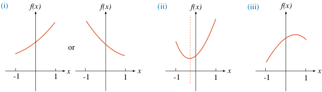
Figure 4: The three cases (i)–(iii) that $f(x)$ becomes nonpositive in the region $-1\leq x\leq 1$.

Here, we present the detailed derivation of the TTS conditions (38a)–(38c) for axisymmetric stationary spacetimes. The problem is reduced to clarifying the condition that

$$f(x)=(k_{2}-k_{1})x^{2}-2v_{1}x+\frac{\hat{r}^{c}D_{c}\alpha}{\alpha}-k_{2}$$ (68)

becomes nonnegative in the interval $[-1,1]$. This parabola has the axis at $x=x_{\rm a}$ with

$$x_{\rm a}=\frac{v_{1}}{k_{2}-k_{1}},$$ (69)

and there, it takes the value

$$f(x_{\rm a})=\frac{\hat{r}^{c}D_{c}\alpha}{\alpha}-k_{2}-\frac{v_{1}^{2}}{k_{2}-k_{1}}.$$ (70)

At the endpoints of the interval $[-1,1]$, $f(x)$ satisfies

$$f(\pm 1)\geq\frac{\hat{r}^{c}D_{c}\alpha}{\alpha}-k_{1}-2|v_{1}|.$$ (71)

The condition can be studied by dividing it into the three cases as indicated in Fig. 4:

• The case that $k_{2}>k_{1}$ and there is no axis in the interval $[-1,1]$, i.e., $|x_{\rm a}|>1$. Since $f(x)$ takes the minimum value at one of the endpoints, we require $f(\pm 1)\geq 0$. This leads to the condition (38a).

• The case that $k_{2}>k_{1}$ and the axis exists in the interval $[-1,1]$, i.e., $|x_{\rm a}|\leq 1$. Since $f(x)$ takes the minimum value at the axis, we require $f(x_{\rm a})\geq 0$. This leads to the condition (38b).

• The case that $k_{2}\leq k_{1}$. Since $f(x)$ takes the minimum value at one of the endpoints, we require $f(\pm 1)\geq 0$. This leads to the condition (38c).

Appendix C Useful geometric formulas

In Sects. 3 and 4, we discussed the connection between the TTS and the LTS and the area bound of TTSs for (i) static and (ii) stationary and axisymmetric cases separately. In this appendix, we will present some useful formulas that have a unified treatment for them and the potential for further generalization to dynamical cases. We can also see the role of the assumption of staticity/stationarity in the argument of the main text.

Here, the setup depicted by Fig. 1 is considered. Specifically, the unit normal $n^{a}$ to the spacelike hypersurface $\Sigma$ is tangent vectors of $S$, and the outward unit normal $\hat{r}^{a}$ to $S$ is tangent to $\Sigma$. First, we derive the general formula without assuming $t^{a}$ to be a Killing field or $t^{a}$ to be tangent to $S$ (unlike the main text of this paper); the discussion here also holds for dynamical setups as long as the above conditions are satisfied. After that, the static case and the axisymmetric stationary case are considered. We also note that the study here concerns the relations between geometric quantities, and the field equations are not explicitly imposed. In addition to the quantities in Fig. 1, we introduce one more geometric quantity, that is, the extrinsic curvature $\bar{k}_{ab}$ of $S_{0}$ in the hypersurface $S$ as defined by $\bar{k}_{ab}=(1/2)\widehat{\pounds}_{n}h_{ab}$. Here, $\widehat{\pounds}$ denotes the Lie derivative in the timelike hypersurface $S$.

C.1 Useful formulas for consideration on LTS

Here, we present the formulas that are useful for considering the connection between the LTS and the TTS. Applying the trace of the Ricci equation to $S_{0}$ as a hypersurface in $S$ and $\Sigma$, respectively, we have

$$R_{ab}n^{a}n^{b} = -\pounds_{n}K-K_{ab}K^{ab}+\frac{1}{\alpha}D^{2}\alpha,$$ (72a)

$$R_{ab}\hat{r}^{a}\hat{r}^{b} = -\pounds_{\hat{r}}\bar{K}-\bar{K}_{ab}\bar{K}^{ab}-\frac{1}{\varphi}\bar{D}^{2}\varphi,$$ (72b)

where $\alpha$ and $\varphi$ are the time and space lapse functions with respect to the $n^{a}$ and $\hat{r}^{a}$ directions, respectively. From these two, one may want to construct

$$\pounds_{\hat{r}}\bar{K}=-\pounds_{n}K-R_{ab}(n^{a}n^{b}+\hat{r}^{a}\hat{r}^{b})-K_{ab}K^{ab}-\bar{K}_{ab}\bar{K}^{ab}+\frac{1}{\alpha}D^{2}\alpha-\frac{1}{\varphi}\bar{D}^{2}\varphi.$$ (73)

Recall the decomposition of $\bar{K}_{ab}$ that is given by Eq. (32) with the vector $v_{a}$ defined in Eq. (33). These formulas also hold in the current setup without assuming staticity/stationarity. The trace of Eq. (32) is

$$\bar{K}=k+\frac{1}{\alpha}\pounds_{\hat{r}}\alpha.$$ (74)

Substituting these formulas together with the decomposition of $D^{2}\alpha$ and $\bar{D}^{2}\varphi$ into lower-dimensional quantities,

$$D^{2}\alpha = \mathcal{D}^{2}\alpha+k\pounds_{\hat{r}}\alpha+\frac{\mathcal{D}_{a}\varphi}{\varphi}\mathcal{D}^{a}\alpha+(\pounds_{\hat{r}})^{2}\alpha,$$ (75a)

$$\bar{D}^{2}\varphi = \mathcal{D}^{2}\varphi-\bar{k}\pounds_{n}\varphi+\mathcal{D}^{a}\varphi\frac{\mathcal{D}_{a}\alpha}{\alpha}-(\pounds_{n})^{2}\varphi,$$ (75b)

we arrive at the general formula for $\pounds_{\hat{r}}k$,

$$\pounds_{\hat{r}}k=-\pounds_{n}K-R_{ab}(n^{a}n^{b}+\hat{r}^{a}\hat{r}^{b})+\frac{1}{\alpha}\mathcal{D}^{2}\alpha-\frac{1}{\varphi}\mathcal{D}^{2}\varphi\\ +k\frac{\pounds_{\hat{r}}\alpha}{\alpha}+\bar{k}\frac{\pounds_{n}\varphi}{\varphi}+\frac{1}{\varphi}(\pounds_{n})^{2}\varphi-K_{ab}K^{ab}-k_{ab}k^{ab}+2v_{a}v^{a}.$$ (76)

Below, we look at the static case and the stationary axisymmetric case, one by one.

C.1.1 Static case

Since $K_{ab}=\pounds_{n}\varphi=v_{a}=0$ for static spacetimes, Eq. (76) becomes

$$\pounds_{\hat{r}}k=-R_{ab}(n^{a}n^{b}+{\hat{r}}^{a}{\hat{r}}^{b})+\frac{1}{\alpha}{\cal D}^{2}\alpha-\frac{1}{\varphi}{\cal D}^{2}\varphi+k\frac{{\pounds}_{\hat{r}}\alpha}{\alpha}-k_{ab}k^{ab}.$$ (77)

This corresponds to Eq. (22) when the Einstein equation holds.

C.1.2 Stationary and axisymmetric case

For stationary and axisymmetric spacetimes, adopting the time slice on which the shift vector $\beta_{a}$ becomes $\beta^{a}=-\omega\phi^{a}$, the extrinsic curvature $K_{ab}$ of $\Sigma$ has the form of Eq. (48), and $v_{a}$ is given as Eq. (35). Since $K=\pounds_{n}\varphi=\phi^{a}D_{a}\omega=\hat{r}^{a}\phi_{a}=0$, Eq. (76) becomes

$$\pounds_{\hat{r}}k=-\frac{\phi^{2}}{2\alpha^{2}}(\mathcal{D}\omega)^{2}-R_{ab}(n^{a}n^{b}+\hat{r}^{a}\hat{r}^{b})+\frac{1}{\alpha}\mathcal{D}^{2}\alpha-\frac{1}{\varphi}\mathcal{D}^{2}\varphi+k\frac{\pounds_{\hat{r}}\alpha}{\alpha}-k_{ab}k^{ab}.$$ (78)

This corresponds to Eq. (52) when the Einstein equation holds. Note that the $t$–$\phi$ orthogonality condition has not been used in deriving this relation.

C.2 Useful formulas for consideration on area bound

Now, we turn our attention to the area bound. As introduced at the beginning of this appendix, $\bar{k}_{ab}$ denotes the extrinsic curvature of $S_{0}$ in $S$. From the double trace of the Gauss equation on $S_{0}$ in $S$, we have

$${}^{(2)}R={}^{(3)}\bar{R}+2{}^{(3)}\bar{R}_{ab}n^{a}n^{b}-\bar{k}^{2}+\bar{k}_{ab}\bar{k}^{ab},$$ (79)

where ${}^{(3)}\bar{R}_{ab}$ is the Ricci tensor with respect to the metric $P_{ab}$ of $S$. Here, ${}^{(3)}\bar{R}$ is written using the double trace of the Gauss equation on $S$ in the spacetime,

$${}^{(3)}\bar{R}=-2G_{ab}\hat{r}^{a}\hat{r}^{b}+\bar{K}^{2}-\bar{K}_{ab}\bar{K}^{ab},$$ (80)

where $G_{ab}$ is the Einstein tensor $G_{ab}:=R_{ab}-(1/2)g_{ab}R$. As for ${}^{(3)}\bar{R}_{ab}n^{a}n^{b}$, one may want to employ the following formula derived by taking trace of the Ricci equation:

$${}^{(3)}\bar{R}_{ab}n^{a}n^{b}=-\pounds_{n}\bar{k}-\bar{k}_{ab}\bar{k}^{ab}+\frac{1}{\alpha}{\cal D}^{2}\alpha.$$ (81)

Here, we used the fact that the hypersurface $S$ has the same time lapse function $\alpha$ as that of the spacetime $\mathcal{M}$ because the timelike unit normal $n^{a}$ is tangent to $S$. Then, Eq. (79) becomes

$${}^{(2)}R=-2\pounds_{n}\bar{k}-2G_{ab}\hat{r}^{a}\hat{r}^{b}+\bar{K}^{2}-\bar{K}_{ab}\bar{K}^{ab}-\bar{k}^{2}-\bar{k}_{ab}\bar{k}^{ab}+\frac{2}{\alpha}\mathcal{D}^{2}\alpha.$$ (82)

Finally, we have the following formula using Eqs. (32) and (74):

$${}^{(2)}R=-2\pounds_{n}\bar{k}-2G_{ab}\hat{r}^{a}\hat{r}^{b}+k^{2}-k_{ab}k^{ab}+2k\frac{\pounds_{\hat{r}}\alpha}{\alpha}+2v_{a}v^{a}-\bar{k}^{2}-\bar{k}_{ab}\bar{k}^{ab}+\frac{2}{\alpha}\mathcal{D}^{2}\alpha.$$ (83)

This is the general formula for ${}^{(2)}R$. We look at the formulas for the static case and the stationary and axisymmetric case, one by one.

C.2.1 Static case

For static cases, $\bar{k}_{ab}=v_{a}=0$ holds, and the above formula then becomes

$${}^{(2)}R=-2G_{ab}\hat{r}^{a}\hat{r}^{b}+k^{2}-k_{ab}k^{ab}+2k\frac{\pounds_{\hat{r}}\alpha}{\alpha}+\frac{2}{\alpha}\mathcal{D}^{2}\alpha.$$ (84)

This corresponds to Eq. (24) when the Einstein equation holds.

C.2.2 Stationary and axisymmetric case

For this case, since $\bar{k}_{ab}={h_{a}}^{c}{h_{b}}^{d}K_{cd}$, we have

$$\bar{k}_{ab}=\frac{1}{2\alpha}(\phi_{a}{\cal D}_{b}\omega+\phi_{b}{\cal D}_{a}\omega)$$ (85)

and $\bar{k}=0$. The formula for $v_{a}$ is given in Eq. (35). Using these formulas, Eq. (83) becomes

$${}^{(2)}R=-2G_{ab}\hat{r}^{a}\hat{r}^{b}+k^{2}-k_{ab}k^{ab}+2k\frac{\pounds_{\hat{r}}\alpha}{\alpha}+\frac{2}{\alpha}\mathcal{D}^{2}\alpha+\frac{\phi^{2}}{2\alpha^{2}}[(\pounds_{\hat{r}}\omega)^{2}-(\mathcal{D}\omega)^{2}].$$ (86)

This corresponds to Eq. (55) when the Einstein equation holds. Note that the $t$–$\phi$ orthogonality property is not necessary in order to derive this formula.

References

- (1) R. Penrose, Annals N. Y. Acad. Sci. 224, 125 (1973).
- (2) P. S. Jang and R. M. Wald, J. Math. Phys. 18, 41 (1977).
- (3) G. Huisken and T. Ilmanen, J. Diff. Geom. 59, 353 (2001).
- (4) H. Bray, J. Diff. Geom. 59, 177 (2001).
- (5) K. S. Virbhadra and G. F. R. Ellis, Phys. Rev. D 62, 084003 (2000) [arXiv:astro-ph/9904193].
- (6) V. Cardoso, E. Franzin and P. Pani, Phys. Rev. Lett. 116, 171101 (2016); Phys. Rev. Lett. 117, 089902 (2016) [erratum] [arXiv:1602.07309 [gr-qc]].
- (7) J. L. Synge, Mon. Not. Roy. Soc. 131, 463 (1966).
- (8) V. Perlick, Living Rev. Relativity 7, 9 (2004).
- (9) C. M. Claudel, K. S. Virbhadra and G. F. R. Ellis, J. Math. Phys. 42, 818 (2001) [arXiv:gr-qc/0005050].
- (10) C. Cederbaum, arXiv:1406.5475 [math.DG].
- (11) C. Cederbaum and G. J. Galloway, arXiv:1504.05804 [math.DG].
- (12) S. Yazadjiev and B. Lazov, Classical Quantum Gravity 32, 165021 (2015) [arXiv:1503.06828 [gr-qc]].
- (13) C. Cederbaum and G. J. Galloway, Classical Quantum Gravity 33, 075006 (2016) [arXiv:1508.00355 [math.DG]].
- (14) S. S. Yazadjiev, Phys. Rev. D 91, 123013 (2015) [arXiv:1501.06837 [gr-qc]].
- (15) S. Yazadjiev and B. Lazov, Phys. Rev. D 93, 083002 (2016) [arXiv:1510.04022 [gr-qc]].
- (16) M. Rogatko, Phys. Rev. D 93, 064003 (2016) [arXiv:1602.03270 [hep-th]].
- (17) H. Yoshino, Phys. Rev. D 95, 044047 (2017) [arXiv:1607.07133 [gr-qc]].
- (18) Y. Tomikawa, T. Shiromizu, and K. Izumi, Prog. Theor. Exp. Phys. 2017, 033E03 (2017) [arXiv:1612.01228 [gr-qc]].
- (19) Y. Tomikawa, T. Shiromizu and K. Izumi, arXiv:1702.05682 [gr-qc].
- (20) G. W. Gibbons and C. M. Warnick, Phys. Lett. B 763, 169 (2016) [arXiv:1609.01673 [gr-qc]].
- (21) E. Teo, Gen. Relativ. Gravit. 35, 1909 (2003).
- (22) T. Shiromizu, Y. Tomikawa, K. Izumi, and H. Yoshino, Prog. Theor. Exp. Phys. 2017, 033E01 (2017) [arXiv:1701.00564 [gr-qc]].
- (23) R. Geroch, Ann. N.Y. Acad. Sci. 224, 108 (1973).
- (24) X. Wang, J. Diff. Geom. 57, 273 (2001).
- (25) R. Wald, General Relativity (The University of Chicago Press, Chicago, 1984).
- (26) A. Gullstrand, Ark. Mat. Astron. Fys 16, 1 (1922).
- (27) B. Carter, Commun. Math. Phys. 17, 233 (1970).
- (28) B. Carter, J. Math. Phys. 10, 70 (1969).
- (29) R. P. Kerr, Phys. Rev. Lett. 11, 237 (1963).
- (30) C. Doran, Phys. Rev. D 61, 067503 (2000) [arXiv:gr-qc/9910099].
- (31) V. P. Frolov and I. D. Novikov, Black Hole Physics: Basic Concepts and New Developments (Kluwer Academic Publishers, Dordrecht and Boston, 1998).
- (32) M. Ansorg and D. Petroff, Phys. Rev. D 72, 024019 (2005) [arXiv:gr-qc/0505060].
- (33) C. A. R. Herdeiro and E. Radu, Phys. Rev. Lett. 112, 221101 (2014) [arXiv:1403.2757 [gr-qc]].
- (34) C. Herdeiro and E. Radu, Class. Quant. Grav. 32, 144001 (2015) [arXiv:1501.04319 [gr-qc]].
- (35) C. Herdeiro, E. Radu and H. Runarsson, Class. Quant. Grav. 33, 154001 (2016) [arXiv:1603.02687 [gr-qc]].
- (36) D. Horvat, S. Ilijic, A. Kirin, and Z. Narancic, Class. Quant. Grav. 30, 095014 (2013) [arXiv:1302.4369 [gr-qc]].
- (37) K. S. Virbhadra and G. F. R. Ellis, Phys. Rev. D 65, 103004 (2002).
- (38) V. Bozza, Phys. Rev. D 66, 103001 (2002) [arXiv:gr-qc/0208075].
- (39) K. S. Virbhadra and C. R. Keeton, Phys. Rev. D 77, 124014 (2008) [arXiv:0710.2333 [gr-qc]].
- (40) S. Sahu, M. Patil, D. Narasimha, and P. S. Joshi, Phys. Rev. D 86, 063010 (2012) [arXiv:1206.3077 [gr-qc]].
- (41) S. Sahu, M. Patil, D. Narasimha, and P. S. Joshi, Phys. Rev. D 88, 103002 (2013) [arXiv:1310.5350 [gr-qc]].
- (42) S. Dain, C. O. Lousto, and R. Takahashi, Phys. Rev. D 65, 104038 (2002) [arXiv:gr-qc/0201062].
- (43) S. Dain and M. Reiris, Phys. Rev. Lett. 107, 051101 (2011) [arXiv:1102.5215 [gr-qc]].
- (44) K. S. Thorne, in Magic without Magic: John Archbald Wheeler, ed. J.Klauder (Freeman, San Francisco, 1972).
- (45) H. Yoshino, Phys. Rev. D 77, 041501 (2008) [arXiv:0712.3907 [gr-qc]].
- (46) H. Saida, A. Fujisawa, C. M. Yoo, and Y. Nambu, Prog. Theor. Exp. Phys. 2016, 043E02 (2016) [arXiv:1503.01840 [gr-qc]].