A Quadratic Penalty Method for Hypergraph Matching

Abstract

Hypergraph matching is a fundamental problem in computer vision. Mathematically, it maximizes a polynomial objective function, subject to assignment constraints. In this paper, we reformulate the hypergraph matching problem as a sparse constrained optimization problem. By dropping the sparse constraint, we show that the resulting relaxation problem can recover the global minimizer of the original problem. This property heavily depends on the special structures of hypergraph matching. The critical step in solving the original problem is to identify the location of nonzero entries (referred to as the support set) in a global minimizer. Inspired by such observation, we apply the quadratic penalty method to solve the relaxation problem. Under reasonable assumptions, we show that the support set of the global minimizer in a hypergraph matching problem can be correctly identified when the number of iterations is sufficiently large. A projected gradient method is applied as a subsolver to solve the quadratic penalty subproblem. Numerical results demonstrate that the exact recovery of the support set indeed happens, and the proposed algorithm is efficient in terms of both accuracy and CPU time.

1 Introduction

Recently, hypergraph matching has become a popular tool in establishing correspondence between two sets of points. It is a central problem in computer vision, and has been used to solve several applications, including object detection berg2005shape , image retrieval yan2005efficient , image stitching zaragoza13 ; zaragoza14 , and bioinformatics wu2012prl .

From the point of view of graph theory, hypergraph matching belongs to bipartite matching. Traditional graph matching models only use point-to-point features or pair-to-pair features, which can be solved by linear assignment algorithms jiang2007 ; maciel2003 or quadratic assignment algorithms egozi2013 ; Jiang2016 ; lee2011 ; litman2014 ; yan2015 , respectively. To use more geometric information such as angles, lines, and areas, triple-to-triple graph matching was proposed in 2008 zass2008probabilistic , and was further studied in duchenne2011tensor ; lee2011hyper ; nguyen2016efficient . Since three vertices are associated with one edge, it is also termed as hypergraph matching. Numerical experiments in literature duchenne2011tensor ; lee2011hyper ; nguyen2016efficient ; zass2008probabilistic show that hypergraph matching is more efficient than traditional graph matching. The aim of this paper is to study the hypergraph matching problem in both theory and algorithm.

The mathematical model of hypergraph matching is to maximize a multi-linear objective function subject to the row permutation constraints for $n_{1}\leq n_{2}$

$$\begin{array}[]{ll}\Pi^{1}=\{X\in\{0,1\}^{n_{1}\times n_{2}}:\sum\limits_{l_{2}=1}^{n_{2}}X_{l_{1}l_{2}}=1,\ l_{1}=1,\ldots,n_{1}\},\end{array}$$ (1.1)

or permutation constraints for $n_{1}=n_{2}$

$$\begin{array}[]{ll}\Pi^{2}=&\{X\in\{0,1\}^{n_{1}\times n_{1}}\,:\ \sum\limits_{l_{2}=1}^{n_{1}}X_{l_{1}l_{2}}=1,\ l_{1}=1,\ldots,n_{1};\\ &\sum\limits_{l_{1}=1}^{n_{1}}X_{l_{1}l_{2}}=1,\ l_{2}=1,\ldots,n_{1}\}.\end{array}$$ (1.2)

We call a matrix satisfying (1.1) or (1.2) a binary assignment matrix. Optimization problems over binary assignment matrices are known to be NP-hard due to the combinatorial property.

Most existing algorithms for hypergraph matching relax the binary constraints into bound constraints and solve a continuous optimization problem. For instance, the probabilistic Hypergraph Matching method (HGM) zass2008probabilistic reformulated the constraints as the intersection of three convex sets, and successively projected the variables onto the sets until convergence. The Tensor Matching method (TM) duchenne2011tensor solved the optimization problem using the power iteration algorithm. The Hypergraph Matching method via Reweighted Random Walks (RRWHM) lee2011hyper dealt with the problem by walking among two feasible vectors randomly. Different from the above algorithms, Block Coordinate Ascent Graph Matching (BCAGM) nguyen2016efficient applied a block coordinate ascent framework, where they kept the binary constraints, and proposed to reformulate the multi-linear objective function into a linear one and solve it using linear assignment algorithms. All the existing algorithms require the equality constraints in (1.1) or (1.2) to be satisfied strictly at each iteration. In fact, we only expect that one of the elements is significantly larger than the others in each row or column of $X$. That is, the equality constraints are only soft constraints, which allow violations to some extent. Therefore, we penalize the equality constraint violations as part of the objective function in our algorithm.

The hypergraph matching problem can also be reformulated equivalently as a nonlinear optimization problem with sparse constraint. During the last few years, in the optimization community, there has been significant progress on solving sparse constrained nonlinear problems, particularly on dealing with optimality conditions and numerical algorithms in different situations. Recent development in optimality conditions can be found in Pan2017 , where based on decomposition properties of the normal cones, the authors characterized different kinds of stationary points and performed detailed investigations on relations of local minimizers, global minimizers and several types of stationary points. Other related work includes Bauschke2014Restricted ; Burdakov2015MATHEMATICAL ; C2016Constraint ; Li2015 ; Pan2015On . The related algorithms can be summarized into two approaches. One is the direct approach, aiming at dealing with the sparse constraint directly, such as the hard-thresholding type based algorithms Beck2012Sparsity ; Pan2016A and the $\ell_{0}$ penalty based algorithms Lu2012Sparse . The other one is the relaxation approach such as the $\ell_{p}$ regularization based algorithms ChenLeiLuYe ; Jiang2016 . In particular, an efficient $\ell_{p}$ regularization algorithm was proposed in Jiang2016 , which deals with problems over the permutation matrix constraints (1.2). It can be applied to solve the hypergraph matching problem subject to (1.2).

Motivation. Noting that hypergraph matching is essentially a mixed integer programming, most existing methods relax the integer constraints as box constraints, and solve the relaxed continuous optimization problem. A natural question is: what is the relation between hypergraph matching and the relaxation problem? Furthermore, the key step in solving this problem is actually to identify the support set of the global minimizer. None of the existing algorithms has taken this fact into account. This leads to the second question: can we make use of this insight to design our algorithm?

Our Contributions. In this paper, by reformulating hypergraph matching equivalently as a sparse constrained optimization problem, we study it from the following aspects.

• Relaxation problem. By dropping the sparse constraint, we show that the relaxation problem can recover the solution of the original problem in the sense that the former problem shares at least one global minimizer with the latter one (Theorem 3.1). This result highly depends on the special structures of hypergraph matching. Furthermore, we show that Theorem 3.1 can be extended to more general problems (Corollary 2). For any global minimizer of the relaxation problem, we propose a procedure to reduce its sparsity until a global minimizer of the original problem is reached.

• Quadratic penalty method. Our aim is to identify the support set of a global minimizer of the original problem, thus the equality constraints are not necessary to be satisfied strictly. This motivates us to penalize the equality constraint violations, and solve the relaxation problem by a quadratic penalty method. We show that under reasonable assumptions, the support set of a global minimizer of the original problem can be recovered exactly, when the number of iteration is sufficiently large (Theorems 4.2 and 4.3).

• Projected gradient method. For the quadratic penalty subproblem, which is a nonlinear problem with simple box constraints, we choose one of the active set based methods called the projected gradient method as a subsolver. The advantage of the active set based method is that it well fits our motivation, which is to identify the support set of the solution rather than to look for the magnitude. Numerical results demonstrate that the exact recovery of the support set indeed happens, and the proposed algorithm is particularly suitable for large-scale problems.

Organization. The rest of the paper is organized as follows. In Section 2, we introduce the reformulation of the hypergraph matching problem, and discuss several preliminary properties. In Section 3, we study the properties of the relaxation problem by dropping the sparse constraint. In Section 4, we study the quadratic penalty method by penalizing the equality constraint violations and establish the convergence results in terms of support set under different situations. An existing projected gradient method is also discussed to solve the quadratic penalty subproblem. Numerical experiments are reported in Section 5. Final conclusions are drawn in Section 6.

Notations. For $x\in\mathbb{R}^{n}$, define the active set as $\mathcal{I}(x)=\{l:\,x_{l}=0\}$ and the support set as $\Gamma(x)=\{l:\,x_{l}>0\}$. We also use $\mathcal{I}^{k}$ and $\Gamma^{k}$, and $\mathcal{I}^{*}$ and $\Gamma^{*}$ to denote the corresponding sets at $x^{k}$ and $x^{*}$, respectively. Let $|\mathcal{I}|$ be the number of elements in the set $\mathcal{I}$. $\|x\|$ denotes the $\ell_{2}$ norm of $x$, $\|x\|_{0}$ the number of nonzero entries in $x$, and $\|x\|_{\infty}$ the infinity norm of $x$.

2 Problem Reformulation

In this section, we will reformulate hypergraph matching as a sparse constrained optimization problem, and discuss several preliminary properties.

2.1 Hypergraph matching problem

In this part, we will give the mathematical formulation for hypergraph matching, including its objective function and constraints.

Consider two hypergraphs $G_{1}=\{V_{1},E_{1}\}$, and $G_{2}=\{V_{2},E_{2}\}$, where $V_{1}$ and $V_{2}$ are sets of points with $|V_{1}|=n_{1}$, $|V_{2}|=n_{2}$, and $E_{1}$, $E_{2}$ are sets of hyperedges. In this paper, we always suppose that $n_{1}\leq n_{2}$, and each point in $V_{1}$ is matched to exactly one point in $V_{2}$, while each point in $V_{2}$ can be matched to arbitrary number of points in $V_{1}$. That is, we focus on (1.1). For each hypergraph, we consider three-uniform hyperedges. Namely, the three points involved in each hyperedge are different, for example, $(l_{1},j_{1},k_{1})\in E_{1}$. Our aim is to find the best correspondence (also referred to as ‘matching’) between $V_{1}$ and $V_{2}$ with the maximum matching score.

Let $X\in\mathbb{R}^{n_{1}\times n_{2}}$ be the assignment matrix between $V_{1}$ and $V_{2}$, i.e.,

$$X_{l_{1}l_{2}}=\left\{\begin{array}[]{ll}1,&\hbox{ if }l_{1}\in V_{1}\hbox{ is assigned to }l_{2}\in V_{2};\\ 0,&\hbox{ otherwise.}\end{array}\right.$$

Two hyperedges $(l_{1},j_{1},k_{1})\in E_{1}$ and $(l_{2},j_{2},k_{2})\in E_{2}$ are said to be matched if $l_{1},j_{1},k_{1}\in V_{1}$ are assigned to $l_{2},j_{2},k_{2}\in V_{2}$, respectively. It can be represented equivalently by $X_{l_{1}l_{2}}X_{j_{1}j_{2}}X_{k_{1}k_{2}}=1$. Let $\mathcal{B}_{l_{1}l_{2}j_{1}j_{2}k_{1}k_{2}}$ be the matching score between $(l_{1},j_{1},k_{1})$ and $(l_{2},j_{2},k_{2})$. Then $\mathcal{B}\in\mathbb{R}^{n_{1}\times n_{2}\times n_{1}\times n_{2}\times n_{1}\times n_{2}}$ is a sixth order tensor. Assume $\mathcal{B}$ is given, satisfying $\mathcal{B}_{l_{1}l_{2}j_{1}j_{2}k_{1}k_{2}}\geq 0$ if $(l_{1},j_{1},k_{1})\in E_{1}$ and $(l_{2},j_{2},k_{2})\in E_{2}$, and $\mathcal{B}_{l_{1}l_{2}j_{1}j_{2}k_{1}k_{2}}=0$, otherwise.

Given hypergraphs $G_{1}=\{V_{1},E_{1}\}$, $G_{2}=\{V_{2},E_{2}\}$, and the matching score $\mathcal{B}$, the hypergraph matching problem takes the following form

$$\max_{X\in\Pi^{1}}\ \ \sum_{\tiny\begin{array}[]{c}(l_{1},j_{1},k_{1})\in E_{1}\\ (l_{2},j_{2},k_{2})\in E_{2}\end{array}}\mathcal{B}_{l_{1}l_{2}j_{1}j_{2}k_{1}k_{2}}X_{l_{1}l_{2}}X_{j_{1}j_{2}}X_{k_{1}k_{2}}.$$ (2.1)

Note that (2.1) is a matrix optimization problem, which can be reformulated as a vector optimization problem as follows.

Let $n=n_{1}n_{2}$, $x\in\mathbb{R}^{n}$ be the vectorization of $X$, that is

$$x:=(\bar{x}_{1}^{T},\ldots,\bar{x}_{n_{1}}^{T})^{T},\ \hbox{with }X=\left[\begin{array}[]{ccc}X_{11}&\cdots&X_{1n_{2}}\\ \vdots&\ddots&\vdots\\ X_{n_{1}1}&\cdots&X_{n_{1}n_{2}}\end{array}\right]:=\left[\begin{array}[]{c }\bar{x}_{1}^{T}\\ \vdots\\ \bar{x}_{n_{1}}^{T}\end{array}\right].$$

Here, $\bar{x}_{i}\in\mathbb{R}^{n_{2}}$ is the $i$-th block of $x$. In the following, for any vector $z\in\mathbb{R}^{n}$, we always assume it has the same partition as $x$. Define $\mathcal{A}\in\mathbb{R}^{n\times n\times n}$ as

$$\mathcal{A}_{ljk}=\mathcal{B}_{l_{1}l_{2}j_{1}j_{2}k_{1}k_{2}},$$ (2.2)

where

$$l=(l_{1}-1)n_{2}+l_{2},\ j=(j_{1}-1)n_{2}+j_{2},\ k=(k_{1}-1)n_{2}+k_{2}.$$ (2.3)

Consequently, (2.1) can be reformulated as

$$\begin{array}[]{rl}\min\limits_{x\in\mathbb{R}^{n}}&\quad f(x):=-\frac{1}{6}\mathcal{A}x^{3}\\ \hbox{s.t.}&\quad e^{T}\bar{x}_{i}=1,\ i=1,\ldots,n_{1},\\ &\quad x\in\{0,1\},\end{array}$$ (2.4)

where $e\in\mathbb{R}^{n_{2}}$ is a vector with all entries equal to one, and $\mathcal{A}x^{3}:=\sum\limits_{l,j,k}\mathcal{A}_{ljk}x_{l}x_{j}x_{k}$.

2.2 Preliminary properties

In this subsection, we will discuss several properties of $\mathcal{A}$, $\mathcal{B}$, and $f(x)$. We begin with properties of $\mathcal{B}$.

Proposition 1

• $\mathcal{B}_{l_{1}l_{2}j_{1}j_{2}k_{1}k_{2}}\geq 0$ for all $l_{1},j_{1},k_{1}=1,\ldots,n_{1}$ and $l_{2},j_{2},k_{2}=1,\ldots,n_{2}$;

• If $(l_{1},j_{1},k_{1})\in E_{1}$, then $l_{1}$, $j_{1}$, and $k_{1}$ are distinct. If $(l_{2},j_{2},k_{2})\in E_{2}$, then $l_{2}$, $j_{2}$, and $k_{2}$ are also distinct;

• For any permutation operator $\pi$, suppose $\pi(l_{1},j_{1},k_{1})=(l_{1}^{\prime},j_{1}^{\prime},k_{1}^{\prime})$ and $\pi(l_{2},j_{2},k_{2})=(l_{2}^{\prime},j_{2}^{\prime},k_{2}^{\prime})$. There is

  $$\mathcal{B}_{l_{1}l_{2}j_{1}j_{2}k_{1}k_{2}}=\mathcal{B}_{l_{1}^{\prime}l_{2}^{\prime}j_{1}^{\prime}j_{2}^{\prime}k_{1}^{\prime}k_{2}^{\prime}}.$$ (2.5)

The above properties of $\mathcal{B}$ result in the following properties of $\mathcal{A}$ directly.

Proposition 2

• $\mathcal{A}_{ljk}\geq 0$, for all $l,j,k=1,\ldots,n$;

• For nonzero entries of $\mathcal{A}$, say $\mathcal{A}_{ljk}$, $x_{l}$, $x_{j}$ and $x_{k}$ come from different blocks of $x$;

• Suppose $(l^{\prime},j^{\prime},k^{\prime})$ is any permutation of $(l,j,k)$. Then

  $$\mathcal{A}_{ljk}=\mathcal{A}_{l^{\prime}j^{\prime}k^{\prime}}.$$ (2.6)

In other words, $\mathcal{A}$ is nonnegative and symmetric.

Proof. (i) follows directly from the nonnegativity of $\mathcal{B}$. In terms of (ii), by the definition of $\mathcal{A}$, there exist $(l_{1},j_{1},k_{1})$ and $(l_{2},j_{2},k_{2})$ such that (2.2) and (2.3) hold. Further, we know that $x_{l}$ is the $l_{2}$-th entry in the $l_{1}$-th block of $x$, i.e., $x_{l}=(\bar{x}_{l_{1}})_{l_{2}}$. Similarly, $x_{j}=(\bar{x}_{j_{1}})_{j_{2}}$ and $x_{k}=(\bar{x}_{k_{1}})_{k_{2}}$. By (ii) in Proposition 1, $l_{1},j_{1},k_{1}$ are distinct, which implies that $x_{l}$, $x_{j}$, $x_{k}$ come from different blocks of $x$. In terms of (iii), since $\pi(l_{1},j_{1},k_{1})=(l_{1}^{\prime},j_{1}^{\prime},k_{1}^{\prime})$, $\pi(l_{2},j_{2},k_{2})=(l_{2}^{\prime},j_{2}^{\prime},k_{2}^{\prime})$, again by the definition of $\mathcal{A}$ and (2.3), there is $B_{l_{1}^{\prime}l_{2}^{\prime}j_{1}^{\prime}j_{2}^{\prime}k_{1}^{\prime}k_{2}^{\prime}}=A_{l^{\prime}j^{\prime}k^{\prime}}$. Together with (2.5) and (2.2), there is (2.6). ∎

Different from other nonlinear problems, the homogenous polynomial $f(x)$ enjoys special structures. To see this, for the $i$-th block $\bar{x}_{i}$, denote

$$x_{-i}=(\bar{x}_{1}^{T},\ldots,\bar{x}_{i-1}^{T},\bar{x}_{i+1}^{T},\ldots,\bar{x}_{n_{1}}^{T})^{T},\ I(i,n_{2})=\{(i-1)n_{2}+1,\ldots,in_{2}\}.$$

Rewrite $f(x)$ as follows:

$$f(x) = -\frac{1}{6}\sum_{l,j,k}\mathcal{A}_{ljk}x_{l}x_{j}x_{k}$$ (2.7)

$$= -\sum_{l\in I(i,n_{2})\hbox{ or }j\in I(i,n_{2})\hbox{ or }k\in I(i,n_{2}),l<j<k}\mathcal{A}_{ljk}x_{l}x_{j}x_{k}$$

$$\quad-\sum_{l,j,k\notin I(i,n_{2}),l<j<k}\mathcal{A}_{ljk}x_{l}x_{j}x_{k}$$

$$:= f^{i}(\bar{x}_{i},x_{-i})+f^{-i}(x_{-i}).$$

Proposition 3

• For each block $\bar{x}_{i}$, $i\in\{1,\ldots,n_{1}\}$, $f(x)$ is a linear function of $\bar{x}_{i}$, i.e., $\nabla_{\bar{x}_{i}}f(x)$ is independent of $\bar{x}_{i}$;

• $$f^{i}(\bar{x}_{i},x_{-i})=\bar{x}_{i}^{T}\nabla_{\bar{x}_{i}}f(x).$$ (2.8)

Proof. In terms of (i), by the definition of $\mathcal{A}$, we only need to consider the term $\mathcal{A}_{ljk}x_{l}x_{j}x_{k}$, where $\mathcal{A}_{ljk}$ is nonzero. Due to (ii) in Proposition 2, $\mathcal{A}_{ljk}x_{l}x_{j}x_{k}$ is linear in each related block $\bar{x}_{l_{1}}$, $\bar{x}_{j_{1}}$, and $\bar{x}_{k_{1}}$. Therefore, $f(x)$ is a linear function of $\bar{x}_{i}$, $i=1,\ldots,n_{1}$.

In terms of (ii), the elements of gradient $\nabla f(x)$ take the following form

$$(\nabla f(x))_{l}=-\sum_{l<j<k}\mathcal{A}_{ljk}x_{j}x_{k}-\sum_{j<l<k}\mathcal{A}_{ljk}x_{j}x_{k}-\sum_{j<k<l}\mathcal{A}_{ljk}x_{j}x_{k}.$$

Rewrite $f^{i}(\bar{x}_{i},x_{-i})$ in (2.7) as

$$f^{i}(\bar{x}_{i},x_{-i})=-\sum_{l\in I(i,n_{2})}\left(\sum_{l<j<k}\mathcal{A}_{ljk}x_{l}x_{j}x_{k}+\sum_{j<l<k}\mathcal{A}_{ljk}x_{l}x_{j}x_{k}+\sum_{j<k<l}\mathcal{A}_{ljk}x_{l}x_{j}x_{k}\right).$$

Hence, $f^{i}(\bar{x}_{i},x_{-i})=\sum\limits_{l\in I(i,n_{2})}x_{l}(\nabla f(x))_{l}$, which gives (2.8). ∎

Equation (2.8) will be useful in Section 3.

2.3 Sparse constrained optimization problem

Problem (2.4) is a 0-1 mixed integer programming, which is one of Karp’s 21 NP-complete problems Karp1972 . In this subsection, we will reformulate (2.4) into a sparse constrained optimization problem.

By direct computations, (2.4) can be reformulated as the following sparse constrained minimization problem

$$\begin{array}[]{rl}\min\limits_{x\in\mathbb{R}^{n}}&f(x)\\ \mathrm{s.t.}&e^{T}\bar{x}_{i}=1,\ i=1,\ldots,n_{1},\\ &x\geq 0,\quad\|x\|_{0}\leq n_{1}.\end{array}$$ (2.9)

To see this, for each $x$ satisfying the equality constraints, we have $\|x\|_{0}\geq n_{1}$. Together with $\|x\|_{0}\leq n_{1}$, we actually have $\|x\|_{0}=n_{1}$.

In particular, if $n_{1}=n_{2}$, by the permutation constraints (1.2), problem (2.9) reduces to the following hypergraph matching problem

$$\begin{array}[]{rl}\min\limits_{x\in\mathbb{R}^{n}}&f(x)\\ \mathrm{s.t.}&e^{T}\bar{x}_{i}=1,\ i=1,\ldots,n_{1},\\ &\hat{e}_{i}^{T}x=1,\ i=1,\ldots,n_{1},\\ &x\geq 0,\quad\|x\|_{0}\leq n_{1},\end{array}$$ (2.10)

where $\hat{e}_{i}=((e^{n_{1}}_{i})^{T},\ldots,(e^{n_{1}}_{i})^{T})^{T}\in\mathbb{R}^{n},$ and $e^{n_{1}}_{i}$ is the $i$-th column of the $n_{1}$-by-$n_{1}$ identity matrix.

Remark 1

Note that the dimension of $x$ is $n=n_{1}n_{2}$, which can be large even for moderate $n_{1}$ and $n_{2}$. For instance, if $n_{1}=100$ and $n_{2}=100$, then $n=10^{4}$, and the number of elements in $\mathcal{A}$ will be around $10^{12}$. Hence, algorithms capable of dealing with large-scale problems are highly in demand.

Remark 2

Problem (2.9) is essentially a $0$-$1$ mixed integer programming. Each feasible point is actually an isolated feasible point, which means that it is a strict local minimizer and of course is a stationary point of (2.9). For a theoretical verification from the optimality point of view, please see Theorems 1 and 3 in an earlier version of our paper CuiLiQiYan2017 .

3 Relaxation Problem of (2.9)

In this section, we will study the relaxation problem (3.1) and its connections with the original problem (2.9).

By dropping the sparse constraint in (2.9), we obtain the following problem (referred to as the relaxation problem)

$$\begin{array}[]{rl}\min\limits_{x\in\mathbb{R}^{n}}&f(x)\\ \mathrm{s.t.}&e^{T}\bar{x}_{i}=1,\ i=1,\ldots,n_{1},\ \ x\geq 0.\end{array}$$ (3.1)

As we will show later in Theorem 3.1, although we drop the sparse constraint, the relaxation problem (3.1) still admits a global minimizer with sparsity $n_{1}$ due to the special structures of (2.9). That is, the relaxation problem (3.1) recovers a global minimizer of (2.9).

Let $\lambda\in\mathbb{R}^{n_{1}},\mu\in\mathbb{R}^{n}$ be the Lagrange multipliers corresponding to the constraints in (3.1). The KKT conditions of (3.1) are

$$\left\{\begin{array}[]{ll}\nabla_{\bar{x}_{i}}f(x)-\lambda_{i}e-\bar{\mu}_{i}=0,\\ \bar{x}_{i}\geq 0,\ \bar{\mu}_{i}\geq 0,\ \bar{x}_{i}^{T}\bar{\mu}_{i}=0,\\ e^{T}\bar{x}_{i}-1=0,\end{array}\right.$$

which are equivalent to

$$\left\{\begin{array}[]{l}\nabla_{\bar{x}_{i}}f(x)-\lambda_{i}e\geq 0,\ \bar{x}_{i}\geq 0,\ (\nabla_{\bar{x}_{i}}f(x)-\lambda_{i}e)^{T}\bar{x}_{i}=0,\\ e^{T}\bar{x}_{i}-1=0,\end{array}\right.$$

for all $i=1,\ldots,n_{1}$. Define the active set and the support set for the $i$-th block $\bar{x}_{i}$ as

$$\mathcal{I}_{i}(x)=\{p:\ (\bar{x}_{i})_{p}=0\},\ \Gamma_{i}(x)=\{p:\ (\bar{x}_{i})_{p}>0\}.$$ (3.2)

The KKT conditions can be reformulated as

$$\left\{\begin{array}[]{lll}(\nabla_{\bar{x}_{i}}f(x))_{p}-\lambda_{i}=0,&\ (\bar{x}_{i})_{p}>0,&\ p\in\Gamma_{i}(x),\\ (\nabla_{\bar{x}_{i}}f(x))_{p}-\lambda_{i}\geq 0,&\ (\bar{x}_{i})_{p}=0,&\ p\in\mathcal{I}_{i}(x),\\ e^{T}\bar{x}_{i}-1=0,&&\end{array}\right.$$ (3.3)

for all $i=1,\ldots,n_{1}$. The above analysis gives the following lemma.

Lemma 1

Let $x\in\mathbb{R}^{n}$ be a stationary point of (3.1), and $\lambda\in\mathbb{R}^{n_{1}}$ be the Lagrange multiplier corresponding to the equality constraints. For all $i=1,\ldots,n_{1}$, we have

• $\lambda_{i}=\min\limits_{p\in\{1,,\ldots,n_{2}\}}(\nabla_{\bar{x}_{i}}f(x))_{p},\hbox{ and }(\nabla_{\bar{x}_{i}}f(x))_{p}=\lambda_{i}$ for $p\in\Gamma_{i}(x)$;

• $f^{i}(\bar{x}_{i},x_{-i})=\lambda_{i}$.

Proof. (i) can be obtained directly from the KKT conditions (3.3).

In terms of (ii), by (2.8), there is

$$f^{i}(\bar{x}_{i},x_{-i}) = (\bar{x}_{i})^{T}\nabla_{\bar{x}_{i}}f(x)$$

$$= \sum_{p\in\Gamma_{i}(x)}(\bar{x}_{i})_{p}(\nabla_{\bar{x}_{i}}f(x))_{p}$$

$$= \sum_{p\in\Gamma_{i}(x)}(\bar{x}_{i})_{p}\lambda_{i}\ \ (\hbox{by (i)})$$

$$= e^{T}{\bar{x}_{i}}\lambda_{i}$$

$$= \lambda_{i},$$

where the last equality is due to $e^{T}\bar{x}_{i}=1$. This completes the proof.∎

Theorem 3.1

There exists a global minimizer $x^{*}$ of (3.1) such that $\|x^{*}\|_{0}=n_{1}$. Furthermore, $x^{*}$ is a global minimizer of (2.9).

Proof. Without loss of generality, let $y^{0}$ be a global minimizer of (3.1) with $\|y^{0}\|_{0}>n_{1}$. Find the first block of $y^{0}$, denoted as $\bar{y}^{0}_{i}$, such that $\|\bar{y}^{0}_{i}\|_{0}>1$. Now we choose one index $p_{0}$ from $\Gamma_{i}(y^{0}):=\{p:(\bar{y}^{0}_{i})_{p}>0\}$, and define a new point $y^{1}=((\bar{y}^{1}_{1})^{T},\ldots,(\bar{y}^{1}_{n_{1}})^{T})^{T}$ as follows:

$$(\bar{y}^{1}_{i})_{p}=\left\{\begin{array}[]{ll}1,&\hbox{ if }p=p_{0};\\ 0,&\hbox{otherwise},\end{array}\right.\ \text{and}\quad\bar{y}^{1}_{i^{\prime}}=\left\{\begin{array}[]{ll}\bar{y}^{1}_{i},&\hbox{ if }i^{\prime}=i;\\ \bar{y}^{0}_{i^{\prime}},&\hbox{otherwise}.\end{array}\right.$$

Then $y^{1}$ is a feasible point for (3.1), and satisfies $y^{1}_{-i}=y^{0}_{-i}$. Furthermore, by Proposition 3, $\nabla_{\bar{x}_{i}}f(x)$ is a function of $x_{-i}$, there is

$$\nabla_{\bar{x}_{i}}f(y^{0})=\nabla_{\bar{x}_{i}}f(y^{1}).$$ (3.4)

Next, we will show that $f(y^{1})=f(y^{0})$. Indeed,

$$f(y^{1})-f(y^{0}) = f^{i}(\bar{y}^{1}_{i},y^{1}_{-i})+f^{-i}(y^{1}_{-i})-f^{i}(\bar{y}^{0}_{i},y^{0}_{-i})-f^{-i}(y^{0}_{-i})$$

$$= f^{i}(\bar{y}^{1}_{i},y^{0}_{-i})+f^{-i}(y^{0}_{-i})-f^{i}(\bar{y}^{0}_{i},y^{0}_{-i})-f^{-i}(y^{0}_{-i})$$

$$= f^{i}(\bar{y}^{1}_{i},y^{1}_{-i})-f^{i}(\bar{y}^{0}_{i},y^{0}_{-i})$$

$$= (\bar{y}^{1}_{i})^{T}\nabla_{\bar{x}_{i}}f(y^{1})-f^{i}(\bar{y}^{0}_{i},y^{0}_{-i})\ (\hbox{by }(\ref{grad-i}))$$

$$= (\bar{y}^{1}_{i})_{p_{0}}(\nabla_{\bar{x}_{i}}f(y^{0}))_{p_{0}}-f^{i}(\bar{y}^{0}_{i},y^{0}_{-i})\ (\hbox{by }(\ref{grad-equal}))$$

$$= \lambda_{i}-\lambda_{i}\ (\hbox{by Lemma \ref{prop-relax1}})$$

$$= 0.$$

This gives that $y^{1}$ is a feasible point with $f(y^{1})=f(y^{0})$. In other words, $y^{1}$ is another global minimizer of (3.1) with $\|y^{1}\|_{0}<\|y^{0}\|_{0}$. If $\|y^{1}\|_{0}=n_{1}$, let $x^{*}:=y^{1}$. Otherwise, by repeating the above process, we can obtain a finite sequence $y^{0},y^{1},\ldots,y^{r}$, which are all feasible points for (3.1) satisfying

$$\|y^{r}\|_{0}<\ldots<\|y^{1}\|_{0}<\|y^{0}\|_{0}.$$

Note that there are $n_{1}$ blocks in $y^{0}\in\mathbb{R}^{n}$. After at most $n_{1}$ steps, the process will stop. In other words, $1\leq r\leq n_{1}$. The final point $y^{r}$ will satisfy $\|y^{r}\|_{0}=n_{1}$. One can obtain a global minimizer $x^{*}:=y^{r}$ of (3.1) with $n_{1}$ nonzero elements.

Next, we will show that $x^{*}$ is also a global minimizer of (2.9). Note that the feasible region of (2.9) is a subset of the feasible region of (3.1). $\|x^{*}\|_{0}=n_{1}$ implies that $x^{*}$ is also a feasible point for (2.9). Together with the fact that $f(x^{*})$ attains the global minimum of (3.1), we conclude that $x^{*}$ is a global minimizer of (2.9). ∎

Theorem 3.1 shows that $\|x^{*}\|_{0}=n_{1}$ is a necessary and sufficient condition for a global minimizer $x^{*}$ of (3.1) to be a global minimizer of (2.9). We highlight this relation in the following corollary.

Corollary 1

A global minimizer $x^{*}$ of (3.1) is a global minimizer of (2.9) if and only if $\|x^{*}\|_{0}=n_{1}$.

A special case of Theorem 3.1 is $|\Gamma_{i}(x^{*})|=1$, for each $i\in\{1,\ldots,n_{1}\}$. Then the global minimizer $x^{*}$ of (3.1) is a global minimizer of (2.9).

Remark 3

From the proof of Theorem 3.1, one can start from any global minimizer $y^{0}$ of (3.1) to reach a point $x^{*}$, which is a global minimizer of both (2.9) and (3.1). We only need to choose one index as the location of nonzero entry in each block $\bar{y}_{i}^{0}$. Assume $p_{i}$ is chosen from $\Gamma_{i}(y^{0})$. Let $\Gamma^{*}_{i}=p_{i}$. This will give the support set in the $i$-th block, which in turn determines the global minimizer $x^{*}$ of (2.9) by

$$(\bar{x}^{*}_{i})_{p}=\left\{\begin{array}[]{ll}1,&\quad\hbox{ if }p=p_{i},\\ 0,&\quad\hbox{otherwise,}\end{array}\right.$$

for each $p\in\{1,\ldots,n_{2}\}$ and $i\in\{1,\ldots,n_{1}\}$. One particular method to choose $p_{i}$ is to choose the index with the largest value within the block. This is actually the projection of $y^{0}$ onto the feasible set of (2.9). Here, we summarize the process in Algorithm 1.

• Given $y=(\bar{y}_{1}^{T},\ldots,\bar{y}_{n_{1}}^{T})^{T}\in\mathbb{R}^{n}$, a global minimizer of (3.1). Let $x=0\in\mathbb{R}^{n}$.

• For all $i=1,\ldots,n_{1}$, find $p_{i}\in\arg\max_{p}(\bar{y}_{i})_{p}$, and let $(\bar{x}_{i})_{p_{i}}=1$.

• Output $x=(\bar{x}_{1}^{T},\ldots,\bar{x}_{n_{1}}^{T})^{T}$, which is a global minimizer of (2.9).

Algorithm 1 The procedure for computing the nearest binary assignment matrix

Note that HGM zass2008probabilistic also solves the relaxation problem (3.1), whereas TM duchenne2011tensor and RRWHM lee2011hyper solve the relaxation problem with the permutation constraints (1.2). However, none of them analyzes the connections between the original problem and the relaxation problem in terms of global minimizers. On contrast, the result in Theorem 3.1 reveals for the first time the connections between the original problem (2.9) and the relaxation problem (3.1), which is one of the main differences of our work from existing algorithms for hypergraph matching.

Theorem 3.1 reveals an interesting connection between the original problem (2.9) and the relaxation problem (3.1) in terms of global minimizers. The result heavily relies on the property of $f(x)$ in Proposition 3, as well as the equality constraints in (2.9). It can be extended to the following general case.

Corollary 2

Consider

$$\begin{array}[]{rl}\min\limits_{x\in\mathbb{R}^{n}}&\hat{f}(x)\\ \mathrm{s.t.}&e^{T}\bar{x}_{i}=\alpha_{i},\ i=1,\ldots,n_{1},\ \ x\geq 0,\end{array}$$ (3.5)

where $\alpha_{i}>0$, and $\bar{x}_{i}\in\mathbb{R}^{m_{i}}$ with $m_{i}$ being positive integers satisfying $\sum_{i=1}^{n_{1}}m_{i}=n$. Suppose that $\hat{f}(x)$ satisfies Proposition 3. Then there exists a global minimizer $x^{*}$ of (3.5) such that $\|x^{*}\|_{0}=n_{1}$. Furthermore, $x^{*}$ is a global minimizer of the following problem

$$\begin{array}[]{rl}\min\limits_{x\in\mathbb{R}^{n}}&\hat{f}(x)\\ \mathrm{s.t.}&e^{T}\bar{x}_{i}=\alpha_{i},\ i=1,\ldots,n_{1},\ \ x\geq 0,\\ &\|x\|_{0}\leq n_{1}.\end{array}$$

4 The Quadratic Penalty Method

In this section, we will consider the quadratic penalty method for the relaxation problem (3.1). It contains three parts. The first part is devoted to motivating the quadratic penalty problem and its preliminary properties. The second part mainly focuses on the quadratic penalty method and the convergence in terms of the support set. In the last part, we apply an existing projected gradient method for the quadratic penalty subproblem.

4.1 The quadratic penalty problem

Note that (3.1) is a nonlinear problem with separated simplex constraints, which can be solved by many traditional nonlinear optimization solvers such as fmincon in MATLAB. As mentioned in Section 1, existing algorithms for hypergraph matching require the equality constraints in (3.1) to be satisfied strictly. On contrast, our aim here is actually to identify the support set of a global minimizer of (3.1) rather than the magnitude. Once the support set is found, we can follow the method in Remark 3 to obtain a global minimizer of (2.9). Inspired by such observations, we penalize the equality constraint violations as part of the objective function. This is another main difference of our method from existing algorithms. It leads us to the following quadratic penalty problem

$$\begin{array}[]{rl}\min\limits_{x\in\mathbb{R}^{n}}&\quad f(x)+\frac{\sigma}{2}\sum_{i=1}^{n_{1}}(e^{T}\bar{x}_{i}-1)^{2}\\ \hbox{s.t.}&\quad x\geq 0,\end{array}$$

where $\sigma>0$ is a penalty parameter. However, this problem is not well defined in general, since for a fixed $\sigma$ the global minimizer will approach infinity. We can add an upper bound to make the feasible set bounded. This gives the following problem

$$\begin{array}[]{rl}\min\limits_{x\in\mathbb{R}^{n}}&\theta(x):=f(x)+\frac{\sigma}{2}\sum_{i=1}^{n_{1}}(e^{T}\bar{x}_{i}-1)^{2}\\ \mathrm{s.t.}&0\leq x\leq M,\end{array}$$ (4.1)

where $M\geq 1$ is a given number. (4.1) is actually the quadratic penalty problem of the following problem

$$\begin{array}[]{rl}\min\limits_{x\in\mathbb{R}^{n}}&f(x)\\ \mathrm{s.t.}&e^{T}\bar{x}_{i}=1,\ i=1,\ldots,n_{1},\ 0\leq x\leq M,\end{array}$$

which is equivalent to (3.1).

Having introduced the quadratic penalty problem (4.1), next we will analyze the properties of (4.1) and its connection with the relaxation problem (3.1).

The Lagrangian function of (4.1) is

$$L(x,w,\nu)=\theta(x)-x^{T}w-(M-x)^{T}\nu,$$

where $w$ and $\nu$ are the Lagrange multipliers corresponding to the inequality constraints in (4.1). The KKT conditions are

$$\left\{\begin{array}[]{l}\nabla_{\bar{x}_{i}}\theta(x)-\bar{w}_{i}+\bar{\nu}_{i}=0,\\ \bar{x}_{i}\geq 0,\ \bar{w}_{i}\geq 0,\ \bar{x}_{i}^{T}\bar{w}_{i}=0,\\ \bar{\nu}_{i}\geq 0,\ M-\bar{x}_{i}\geq 0,\ \bar{\nu}_{i}^{T}(M-\bar{x}_{i})=0,\end{array}\right.$$

for each $i\in\{1,\ldots,n_{1}\}$. In particular, for a stationary point $x$ of (4.1), let $\mathcal{I}_{i}(x)$ and $\Gamma_{i}(x)$ be defined by (3.2). Define

$$\widehat{\Gamma}_{i}(x)=\{p:(\bar{x}_{i})_{p}\in(0,M),p\in\Gamma_{i}(x)\},\ \overline{\Gamma}_{i}(x)=\{p:(\bar{x}_{i})_{p}=M,p\in\Gamma_{i}(x)\}.$$

The KKT conditions are equivalent to the following, for each $i\in\{1,\ldots,n_{1}\}$,

$$\left\{\begin{array}[]{ll}(\nabla_{\bar{x}_{i}}f(x))_{p}+\sigma(e^{T}\bar{x}_{i}-1)\geq 0,\ (\bar{x}_{i})_{p}=0,&p\in\mathcal{I}_{i}(x),\\ (\nabla_{\bar{x}_{i}}f(x))_{p}+\sigma(e^{T}\bar{x}_{i}-1)=0,\ (\bar{x}_{i})_{p}\in(0,M),&p\in\widehat{\Gamma}_{i}(x),\\ (\nabla_{\bar{x}_{i}}f(x))_{p}+\sigma(e^{T}\bar{x}_{i}-1)\leq 0,\ (\bar{x}_{i})_{p}=M,&p\in\overline{\Gamma}_{i}(x).\end{array}\right.$$ (4.2)

Define the violations of the equality constraints $h\in\mathbb{R}^{n_{1}}$ as

$$h_{i}=e^{T}\bar{x}_{i}-1,\ i=1,\ldots,n_{1}.$$ (4.3)

There is

$$\sigma h_{i}\in\left[-\max_{p\in\{1,\ldots,n_{2}\}}(\nabla_{\bar{x}_{i}}f(x))_{p},\ -\min_{p\in\{1,\ldots,n_{2}\}}(\nabla_{\bar{x}_{i}}f(x))_{p}\right].$$ (4.4)

The above analysis can be stated in the following lemma.

Lemma 2

Let $x\in\mathbb{R}^{n}$ be a stationary point of (4.1). We have $h_{i}\geq 0$ for all $i=1,\ldots,n_{1}$.

Proof. For each $i$, consider two cases. If $\mathcal{I}_{i}(x)\cup{\widehat{\Gamma}}_{i}(x)\neq\emptyset$, by (4.2), there exists $p\in\mathcal{I}_{i}(x)\cup{\widehat{\Gamma}}_{i}(x)$ such that $\sigma h_{i}\geq-(\nabla_{\bar{x}_{i}}f(x))_{p}$. By the nonnegativity of the entries in $\mathcal{A}$ and $x$, there is $-\nabla_{\bar{x}_{i}}f(x)\geq 0$ and $h_{i}\geq 0$. If $\mathcal{I}_{i}(x)\cup{\widehat{\Gamma}}_{i}(x)=\emptyset$, then $|\overline{\Gamma}_{i}(x)|=n_{2}$. In other words, $(\bar{x}_{i})_{p}=M$ for all $p=1,\ldots,n_{2}$. Then $h_{i}=e^{T}\bar{x}_{i}-1=n_{2}M-1\geq 0$. ∎

Let $u\in\mathbb{R}^{n}$ and $c\in\mathbb{R}^{n_{1}}$ be defined by

$$u_{l}=\sum_{l<j<k}\mathcal{A}_{ljk}+\sum_{j<l<k}\mathcal{A}_{ljk}+\sum_{j<k<l}\mathcal{A}_{ljk},\ \ l=1,\ldots,n,$$

and

$$c_{i}:=M^{2}\max_{p\in\{1,\ldots,n_{2}\}}(\bar{u}_{i})_{p},\ i=1,\ldots,n_{1},$$ (4.5)

where $\bar{u}_{i}$ is the $i$-th block of $u$. It follows from the nonnegativity of $\mathcal{A}$ that $c\geq 0$. The following lemma describes the relation between the penalty parameter $\sigma$ and the violations of the equality constraints.

Lemma 3

For each stationary point $x$ of (4.1), there is

$$h_{i}\leq\frac{c_{i}}{\sigma},\ \forall\ i=1,\ldots,n_{1},$$

where $h_{i}$ is defined by (4.3), and $c_{i}$ is defined by (4.5).

Proof. Note that $x\in[0,M]$. By the definition $f(x)=-\frac{1}{6}\mathcal{A}x^{3}$, we have $-(\nabla f(x))_{l}\leq M^{2}u_{l}.$ Together with (4.4), there is $\sigma h_{i}$$\leq M^{2}\max_{p\in\{1,\ldots,n_{2}\}}(\bar{u}_{i})_{p}$ $=c_{i}$. The proof is complete. ∎

Lemma 4

For each feasible point $x\in\mathbb{R}^{n}$ of (3.1), it is a stationary point of (4.1) if and only if for all $i=1,\ldots,n_{1}$, there is

$$(\nabla_{\bar{x}_{i}}f(x))_{p}=0,\ \forall\ p\in\mathcal{I}_{i}(x)\cup\widehat{\Gamma}_{i}(x).$$ (4.6)

Proof. Let $x$ be a feasible point for (3.1). There is $e^{T}\bar{x}_{i}-1=0$, $i=1,\ldots,n_{1}$. If $x$ is a stationary point of (3.1), by the KKT conditions (4.2), we have

$$(\nabla_{\bar{x}_{i}}f(x))_{p}+\sigma(e^{T}\bar{x}_{i}-1)\geq 0,\ (\bar{x}_{i})_{p}=0,\ p\in\mathcal{I}_{i}(x),\ i=1,\ldots,n_{1}.$$

Consequently, $(\nabla_{\bar{x}_{i}}f(x))_{p}\geq-\sigma(e^{T}\bar{x}_{i}-1)=0$. On the other hand, $(\nabla_{\bar{x}_{i}}f(x))_{p}\leq 0$ due to the nonnegativity of entries in $\mathcal{A}$ and $x$. Therefore, $(\nabla_{\bar{x}_{i}}f(x))_{p}=0$ for all $p\in\mathcal{I}_{i}(x)$. For $p\in\Gamma_{i}(x)$, there is $(\nabla_{\bar{x}_{i}}f(x))_{p}=0.$ This gives (4.6).

Conversely, for a feasible point $x$ for (2.9), if (4.6) holds, the first two conditions in (4.2) hold by $\bar{x}_{i}^{T}e-1=0$, $i=1,\ldots,n_{1}$. For the third condition in (4.2), consider two cases. If $\overline{\Gamma}(x)=\emptyset,$ the result is trivial. Otherwise, there is $(\nabla_{\bar{x}_{i}}f(x))_{p}\leq 0$ due to the nonnegativity of entries in $\mathcal{A}$ and $x$. The third condition holds automatically. In both two cases, $x$ satisfies (4.2). That is, $x$ is a stationary point of (4.1). ∎

4.2 A quadratic penalty method for (3.1)

Having investigated the properties of the quadratic penalty problem, we then solve (3.1) by the traditional quadratic penalty method, i.e., by solving (4.1) sequentially. At each iteration, $x^{k}$ is a global minimizer of the following problem

$$(P_{k})\ \ \min_{0\leq x\leq M}\ \theta^{k}(x):=f(x)+\frac{\sigma_{k}}{2}\sum_{i=1}^{n_{1}}(e^{T}\bar{x}_{i}-1)^{2}.$$ (4.7)

The quadratic penalty method is given in Algorithm 2.

• Given an initial point $x^{0}\geq 0$, set the parameter $\sigma_{0}>0$. Let $k:=1$.

• Start from $x^{k-1}$ and solve ($P_{k}$) in (4.7) to obtain a global minimizer $x^{k}$.

• If the termination rule is satisfied, project $x^{k}$ to $\Pi^{1}$ in (1.1) by Algorithm 1. Otherwise, choose $\sigma_{k+1}\geq\sigma_{k}$, $k=k+1$, and go to Step 1.

Algorithm 2 Quadratic penalty method for (3.1)

The following theorem addresses the convergence of the quadratic penalty method, which can be found in classic optimization books such as (NumericalOpt, , Theorem 17.1) and (SunYuan, , Corollary 10.2.6). Therefore, the proof is omitted.

Theorem 4.1

Let $\{x^{k}\}$ be generated by Algorithm 2, and $\lim_{k\to\infty}\sigma_{k}=+\infty$. Then any accumulation point of the generated sequence $\{x^{k}\}$ is a global minimizer of (3.1).

Due to Theorem 4.1, in following analysis, we always assume the following holds.

Assumption 1

Let $\{x^{k}\}$ be generated by Algorithm 2 and $\lim_{k\rightarrow\infty}\sigma_{k}=+\infty$. Denote $K$ as a subset of $\{1,2,\ldots\}$. Assume that $\lim_{k\rightarrow\infty,k\in K}x^{k}=z$, and $z$ is a global minimizer of (3.1).

The next theorem mainly addresses the relation between the support set of $x^{k}$ and that of the global minimizer of (2.9). Recall that for $x^{k}$, there is

$$\mathcal{I}^{k}=\{l:\ x_{l}^{k}=0\},\ \ \Gamma^{k}=\{l:\ x_{l}^{k}>0\}.$$

Theorem 4.2

Suppose that Assumption 1 holds. If there exists a positive integer $k_{0}$, such that $\|x^{k}\|_{0}=n_{1}$ for all $k\geq k_{0},\ k\in K$, then there is a positive integer $k_{1}\geq k_{0}$ such that the support set of $z$ can be identified correctly. That is,

$$\Gamma^{k}=\Gamma(z),\ \text{for all}\ k\geq k_{1},\ k\in K.$$

Furthermore, $z$ is a global minimizer of (2.9).

Proof. First, we show $|\Gamma(z)|=n_{1}$. Noting that $z$ is a global minimizer of (4.1), we have

$$\Gamma(z)\geq n_{1}.$$

Since $\lim_{k\to+\infty,k\in K}x^{k}=z$, there exists a positive integer $k^{\prime}$ such that for $k\geq k^{\prime},\ k\in K$, there is

$$x^{k}_{l}>1/2,\text{ for all }l\in\Gamma(z).$$

This implies that $\Gamma(z)\subseteq\Gamma^{k}$. It follows from the assumption that $|\Gamma^{k}|=n_{1}$ for all $k\geq k_{0},\ k\in K$. Consequently, we have $|\Gamma(z)|=n_{1}$. Therefore, $\Gamma(z)=\Gamma^{k}$ holds for $k\geq k_{1}:=\max\{k_{0},k^{\prime}\}$. The second part holds following the second part of Theorem 3.1. The proof is finished.∎

Theorem 4.2 indicates that we do not need to drive $\sigma_{k}$ to infinity since only the support set of $z$ is needed. If the conditions in Theorem 4.2 hold, then we can stop the algorithm when the number of elements in $\mathcal{I}^{k}$ keeps unchanged for several iterations. However, if there is $\|x^{k}\|_{0}>n_{1}$, we need more notations to analyze the connections.

Let $\mathcal{J}^{k}_{i}$ be the set of indices corresponding to the largest values in the $i$-th block $\bar{x}^{k}_{i}$, $p^{k}_{i}$ be the smallest index in $\mathcal{J}^{k}_{i}$, and $\mathcal{J}^{k}$ be the set of indices containing the largest values in each block of $x^{k}$, i.e.,

$$\mathcal{J}^{k}_{i}=\arg\max_{p}\{(\bar{x}^{k}_{i})_{p}\},\ p^{k}_{i}=\min\{p:p\in\mathcal{J}^{k}_{i}\},\hbox{ and }\mathcal{J}^{k}:=\bigcup_{i=1}^{n_{1}}\{p_{i}^{k}+n_{2}(i-1)\}.$$

Similarly, we define

$$\mathcal{J}_{i}(z)=\arg\max_{p}\{(\bar{z}_{i})_{p}\},\ p_{i}(z)=\min\{p:p\in\mathcal{J}_{i}(z)\},\ \mathcal{J}(z):=\bigcup_{i=1}^{n_{1}}\{p_{i}(z)+n_{2}(i-1)\}.$$

Theorem 4.3

Suppose that Assumption 1 holds.

• If $\|z\|_{0}=n_{1}$, then there exists an integer $k_{0}>0$, such that $\Gamma(z)=\mathcal{J}^{k}$ for all $k\geq k_{0},\ k\in K$;

• If $\|z\|_{0}>n_{1}$ and $|\mathcal{J}_{i}(z)|=1$ for all $i=1,\ldots,n_{1}$, then there exists a global minimizer $x^{*}$ of (2.9) and a positive integer $k_{0}$, such that for all $k\geq k_{0},k\in K$, there is $\Gamma^{*}=\mathcal{J}^{k}$;

• If $\|z\|_{0}>n_{1}$ and $|\mathcal{J}_{i}(z)|>1$ for one $i=1,\ldots,n_{1}$, then there exists a global minimizer $x^{*}$ of (2.9), a subsequence $\{x^{k}\}_{k\in K^{\prime}}$ and a positive integer $k_{0}$, such that for all $k\geq k_{0},k\in K^{\prime}$, there is $\Gamma^{*}=\mathcal{J}^{k}$.

Proof. With Theorem 3.1 and $\|z\|_{0}=n_{1}$, $z$ must be a global minimizer of (2.9). By the definition of $\Gamma(z)$ and $\mathcal{I}(z)$, there exists an integer $k_{0}>0$, such that for all $k\geq k_{0},k\in K$, there is $z_{l}>z_{l^{\prime}}$ for ${l^{\prime}}\in\mathcal{I}(z)$ and $l\in\Gamma(z)$. This gives $\mathcal{J}^{k}_{i}=\mathcal{J}_{i}(z)$ and (i).

In terms of (ii), $|\mathcal{J}_{i}(z)|=1$ implies that for $k\in K$ sufficiently large, there is

$$(\bar{x}^{k}_{i})_{\mathcal{J}_{i}(z)}>(\bar{x}^{k}_{i})_{p},\ \forall\,p\notin\mathcal{J}_{i}(z),\ \ i=1,\ldots,n_{1}.$$

Consequently, there is $\mathcal{J}^{k}_{i}=\mathcal{J}_{i}(z)$. Now let $y^{0}:=z$. Similar to the arguments in the proof of Theorem 3.1, we construct $y^{1}$ by choosing $p_{0}=\mathcal{J}_{i}(z)$. Then we can obtain a finite sequence $y^{0},y^{1},\ldots,y^{r}$ with

$$\|y^{r}\|_{0}<\ldots<\|y^{1}\|_{0}<\|y^{0}\|_{0}.$$

After at most $n_{1}$ steps, the process will stop. In other words, $1\leq r\leq n_{1}$. At the final point $y^{r}$ will satisfy $\|y^{r}\|_{0}=n_{1}$. One can find a global minimizer $x^{*}:=y^{r}$ of problem (3.1) with sparsity $n_{1}$. Further, $x^{*}$ is also a global minimizer of (2.9) and satisfies

$$|\mathcal{J}^{*}_{i}|=1,\ \mathcal{J}_{i}^{*}=\Gamma_{i}^{*}=\mathcal{J}_{i}(z)=\mathcal{J}_{i}^{k}.$$

Consequently, (ii) holds.

For (iii), suppose there exists an index $q_{1}$ such that $|\mathcal{J}_{q_{1}}(z)|>1$. Consequently, there exists $p_{1}\in\mathcal{J}^{k}_{q_{1}}$, such that for $k\in K$ sufficiently large, there are infinite number of $k$ satisfying $\mathcal{J}_{q_{1}}^{k}=p_{1}$. Denote the corresponding subsequence as $\{x^{k}\}_{k\in K_{1}}$, where $K_{1}\subset K$. Similarly, for $|\mathcal{J}_{q_{2}}(z)|>1$, we can find an infinite number of $k\in K_{2}\subseteq K_{1}$ such that $\mathcal{J}_{q_{2}}^{k}=p_{2}$. Repeating the process until for all blocks, there exists an integer $k_{0}>0$, such that $|\mathcal{J}_{i}^{k}|=1$, $i=1,\ldots,n_{1}$, for all $k\in K_{t}\subseteq K_{t-1}\ldots\subseteq K_{1}$, $k\geq k_{0}$. Let $K^{\prime}:=K_{t}$. Now similar to Remark 3, for all $i=1,\ldots,n_{1}$, we define $x^{*}$ as follows:

$$(\bar{x}^{*}_{i})_{p_{i}}=\left\{\begin{array}[]{ll}1,&\hbox{ if }{p_{i}}=\mathcal{J}_{i}^{k},\ k\in K^{\prime},\ k\geq k_{0},\\ 0,&\hbox{ otherwise.}\end{array}\right.$$

Then we find a global minimizer of (3.1) such that $\|x^{*}\|_{0}=n_{1}$. For $k\geq k_{0}$, $k\in K^{\prime}$, there is $\mathcal{J}_{i}^{k}=\mathcal{J}_{i}^{*}$, $i=1,\ldots,n_{1}$. Consequently, $x^{*}$ is also a global minimizer of (2.9). Hence, (iii) holds. This completes the proof. ∎

Theorems 4.2 and 4.3 state that there is always a subsequence of $x^{k}$ whose support set will coincide with the support set of one global minimizer of (2.9). Consequently, it provides a method to design the termination rule for Algorithm 2.

4.3 A projected gradient method for the subproblem (4.1)

In this subsection, we will use a projected gradient method to solve the subproblem.

Note that the subproblem (4.1) is a nonlinear problem with simple box constraints. Various methods can be chosen to solve (4.1), one of which is the active set based method. We prefer such type of method because it quite fits our motivation to identify the support set of the global minimizer of (2.9) rather than the magnitude. The strategy of identifying the active set is therefore crucial in solving (4.1). We choose a popular approach proposed in Bertsekas1982Bertsekas , and modify it into the resulting projected gradient method, as shown in Algorithm 3. Other typical projected gradient methods in calamai1987 ; dai2006 can also be used.

Remark 4

Note that the projected gradient method is only guaranteed to converge to a stationary point. Based on Lemma 2, the sum of each block in the stationary point is larger than or equal to one. In other words, at least one entry in each block is larger than zero. This will partly explain the numerical observation that the magnitudes of the returned solution by our algorithm clearly fall into two parts: the estimated active part, which is close to zero, and the estimated nonzero part. The latter part is actually the estimated support set where the true support set of global minimizers of (2.9) lies in. Moreover, based on Remark 3, one could identify the support set of a global minimizer of (2.9) easily. On the other hand, noting that the quadratic penalty problem (4.1) is in general nonconvex, it is usually not easy to find a global minimizer. Fortunately, our numerical results demonstrate that in many cases, the projected gradient method can return a solution with accurate support set.

Note that the relaxation problem (3.1) does not take any sparsity into account. However, as shown in Theorem 3.1 at least one of the global minimizers of the relaxation problem (3.1) is a global minimizer of the original problem (2.9). By the quadratic penalty method, we can indeed identify the support set of one global minimizer of (2.9) under reasonable assumptions.

Remark 5

We focused on the problem (2.9) so far. One may wonder whether the theoretical results can be extended to (2.10). It turns out that the extension is not trivial and the analysis becomes more challenging and complicated due to the equality constraints $e^{T}\bar{x}_{i}-1=0$ and $\hat{e}_{i}^{T}x-1=0$. We leave it as a topic to study in future. However, as we will demonstrate in the numerical part, the algorithm designed here can also be applied to solving the relaxation problem of (2.10).

• Given an initial point $x^{0}\in\mathbb{R}^{n}$ with $0\leq x^{0}\leq M$ and tolerance $\hbox{Tol}>0$. Set the parameters as $0<\rho<1/2$, $\epsilon>0$, $0<\beta<1$, $M\geq 1$. Let $j:=0.$ Denote $P(x)$ as the projection of $x\in\mathbb{R}^{n}$ onto the box constraint $0\leq x\leq M$, and $g(x)=\nabla\theta(x)$.

• Calculate the estimated active set at $x^{j}$ as

  $$I_{j}:=\left\{l\;|\;0\leq x_{l}^{j}\leq\epsilon^{j},\;g_{l}(x^{j})>0;\ \hbox{or }M-\epsilon^{j}\leq x^{j}_{l}\leq M,\;g_{l}(x^{j})<0;\;l=1,\ldots,n\right\},$$

  where $\epsilon^{j}=\min\{\epsilon,\omega^{j}\}$, $\omega^{j}=\|x^{j}-P(x^{j}-Ng(x^{j}))\|$, and $N$ is a fixed positive definite diagonal matrix in $\mathbb{R}^{n\times n}$. Let $\bar{I}_{j}:=\{1,\ldots,n\}\backslash I_{j}$.

• Calculate the residual $\delta^{j}\in\mathbb{R}^{n}$ by

  $$\delta^{j}:=\left[\begin{array}[]{l}\delta^{j}_{I_{j}}\\ \delta^{j}_{\bar{I}_{j}}\end{array}\right]$$

  with $\delta^{j}_{I_{j}}=\min\left\{x^{j}_{I_{j}},\;g_{{I_{j}}}(x^{j})\right\}$ and $\delta^{j}_{\bar{I}_{j}}=g_{{\bar{I}_{j}}}(x^{j})$. If $\|\delta^{j}\|\leq\hbox{Tol}$, stop. Otherwise, go to Step 3.

• Calculate the direction $d^{j}\in\mathbb{R}^{n}$ by

  $$d^{j}:=\left[\begin{array}[]{l}d^{j}_{I_{j}}\\ d^{j}_{\bar{I}_{j}}\end{array}\right]$$

  where $d^{j}_{I_{j}}=-(Z^{j})^{-1}x_{I_{j}}$, $Z^{j}\in\mathbb{R}^{|I_{j}|\times|I_{j}|}$ is a positive definite diagonal matrix, and $d^{j}_{\bar{I}_{j}}=-\eta^{j}g_{{I_{j}}}(x^{j})$, where $\eta^{j}$ is a scaling parameter.

• Choose the step size as $\alpha^{j}=\beta^{m^{j}}$, where $m^{j}$ is the smallest nonnegative integer $m$ such that the following condition holds

  $$\theta(P(x^{j}+\beta^{m}d^{j}))-\theta(x^{j})\leq\rho\left(\beta^{m}\sum_{l\in\bar{I}_{j}}g_{l}(x^{j})d^{j}_{l}+\sum_{l\in I_{j}}g_{l}(x^{j})(P(x^{j}_{l}+\beta^{m}d^{j}_{l})-x_{l}^{j})\right).$$

• Update $x^{j+1}$ by $x^{j+1}=P(x^{j}+\alpha^{j}d^{j})$, $j:=j+1$. Go to Step 1.

Algorithm 3 Projected gradient method

5 Numerical Results

In this section, we will evaluate the performance of our algorithm and compare it with several state-of-the-art approaches for hypergraph matching.

5.1 Implementation issues

Our algorithm is termed as QPPG, which is the abbreviation of Quadratic Penalty Projected Gradient method. Basically, we run Algorithm 2 (referred to as outer iterations) and solve the subproblem (4.7) by calling Algorithm 3 (referred to as inner iterations). In practice, we only execute an inexact version of Algorithm 2 by one step. QPPG2 means that Algorithm 2 is applied to permutation constraints (1.2). For TM duchenne2011tensor , RRWHM lee2011hyper , HGM zass2008probabilistic , and BCAGM nguyen2016efficient , we use the authors’ MATLAB codes and C++ mex files. Our algorithm is implemented in MATLAB (R2015a), while tensor vector multiplications are computed with C++ mex files. All the experiments are preformed on a Dell desktop with Intel dual core i7-4770 CPU at 3.40 GHz and 8GB of memory running Windows 7.

In Algorithm 2, set $\sigma_{0}=10$ and the initial point $x^{0}$ as the vector with all entries equal to one. Update $\sigma_{k}$ as

$$\sigma_{k+1}=\left\{\begin{array}[]{ll}\min(10^{5},1.3\sigma_{k}),&\hbox{ if }\sum_{i}|h_{i}^{k}|\geq 0.1;\\ \min(10^{5},1.2\sigma_{k}),&\hbox{ if }\underline{h}^{k}\leq\sum_{i}|h_{i}^{k}|<0.1;\\ \sigma_{k},&\hbox{ otherwise,}\end{array}\right.$$ (5.1)

where $h_{i}^{k}=e^{T}\bar{x}_{i}^{k}-1$ and $\underline{h}^{k}$ is the maximal value of $\sum_{i}|h_{i}^{k}|$ for five consecutive steps. We stop Algorithm 2 if one of the following conditions is satisfied: (a) $|\Gamma^{k}|$ is less than $1.2n_{1}$; (b) $|\Gamma^{k}|$ stays unchanged for ten consecutive steps. As for the output, each $x^{k}$ returned by different algorithms is projected to its nearest binary assignment matrix by Algorithm 1 except HGM and BCAGM, which output a binary assignment matrix directly). The parameters in Algorithm 3 are $\hbox{Tol}=10^{-5}$, $\rho=10^{-6}$, $\epsilon=10^{-2}$, and $\beta=0.5$. $\eta^{j}$ is chosen as $\eta^{j}=\frac{n_{1}}{\|g_{\bar{I}_{j}}(x^{j})\|_{\infty}}$. The positive definite diagonal matrices $N$ and $Z^{j}$ are set to be the identity matrix.

Generating Tensor $\mathcal{A}$. Note that $\mathcal{A}\in\mathbb{R}^{n\times n\times n}$ contains $n^{3}$ elements. Fortunately, in hypergraph matching, as analyzed in Proposition 2, $\mathcal{A}$ has special structures. Further, $\mathcal{A}$ is also sparse. There are three steps to generate $\mathcal{A}$. The first step is to construct hyperedges $E_{1}$ and $E_{2}$, where each hyperedge connects three different points. The hyperedges in $E_{1}$ are generated by randomly selecting three points in $V_{1}$. We fix $|E_{1}|$ as $n$. $E_{2}$ contains the nearest triples to elements in $E_{1}$, and is generated following the nearest neighbour query approach in duchenne2011tensor ; nguyen2016efficient . The second step is to generate $\mathcal{B}$. Note that the number of nonzero entries in $\mathcal{B}$ are at most $|E_{1}||E_{2}|$, which will be large even for moderate $|E_{1}|$ or $|E_{2}|$. In fact, for each hyperedge in $E_{1}$, we only use $s$ nearest hyperedges in $E_{2}$ to construct $\mathcal{B}$. In other words, $\mathcal{B}$ is calculated by

$$\mathcal{B}_{l_{1}l_{2}j_{1}j_{2}k_{1}k_{2}}=\left\{\begin{array}[]{ll}\exp\{-\gamma\|f_{l_{1}j_{1}k_{1}}-f_{l_{2}j_{2}k_{2}}\|\},&\hbox{ if }(l_{2},j_{2},k_{2})\in E_{2}\hbox{ is one of the }s\\ &\hbox{ nearest neighbours of }(l_{1},j_{1},k_{1}),\\ 0,&\hbox{ otherwise,}\end{array}\right.$$ (5.2)

where $f_{l_{1}j_{1}k_{1}}$ and $f_{l_{2}j_{2}k_{2}}$ are feature vectors determined by hyperedges $(l_{1},j_{1},k_{1})$ and $(l_{2},j_{2},k_{2})$, and $\gamma=\frac{1}{\text{mean}(\|f_{l_{1}j_{1}k_{1}}-f_{l_{2}j_{2}k_{2}}\|)}$ is a normalization parameter. Here, for each $(l_{1},j_{1},k_{1})\in E_{1}$, the $s$ nearest neighbours are the $s$ smallest solutions for $\min_{(l_{2},j_{2},k_{2})\in E_{2}}\|f_{l_{1}j_{1}k_{1}}-f_{l_{2}j_{2}k_{2}}\|$. Then $\mathcal{A}$ can be obtained according to (2.2). The number of nonzero elements is $O(sn)$, which is linear in $n$. Therefore, $\mathcal{A}$ is a sparse tensor.

We evaluate the numerical performance mainly from the following three aspects: (1) ‘Accuracy’: denoting the ratio of successful matching, calculated by

$$\frac{\hbox{number of correctly identified support indices }}{\hbox{number of true support indices}};$$

(2) ‘Matching Score’: calculated by $\frac{1}{6}\mathcal{A}(x_{B}^{k})^{3}$, where $x_{B}^{k}$ is the nearest binary assignment vector of $x^{k}$ generated by Algorithm 1; (3) ‘Running Time’: the total CPU time in seconds. For each algorithm (except BCAGM), we only count the computing time for solving the optimization problem. However, BCAGM has to compute all elements in $\mathcal{A}$ to obtain results with high accuracy. Therefore, the running time for BCAGM contains two parts: generating $\mathcal{A}$ with all elements and solving the optimization problem.

Role of Sparsity of $\mathcal{A}$. To see this, we test different values of $s$ on the examples from the CMU house dataset, which has been widely used in literature duchenne2011tensor ; lee2011hyper ; nguyen2016efficient ; zhou2015local . For all examples, there is $n_{1}=30$ and $n_{2}=30$. We take all 111 pictures with labels from 0 to 110, which are the same house taken from slightly different viewpoints. That is, two houses with close labels are similar. For each picture with label $v_{1}$, we match it with $v_{1}+60$. In other words, matching picture $v_{1}$ with $v_{1}+60$ is a test problem. Then we change $v_{1}$ from $0$ to $50$ to produce $51$ test examples. To save time of generating input data $\mathcal{A}$, only elements with $l\leq j\leq k$ are computed in $\mathcal{A}$, and the time consumed is denoted by ‘GTensor’. The average results for the test examples are reported in Figure 5.1. One can see that CPU time for generating tensor is not neglectble comparing with CPU time for solving the problem. On the other hand, the accuracy stays almost unchanged for $s\geq 100$. Note that the matching score will be larger when $s$ increases. It is reasonable as a denser $\mathcal{A}$ will result in a larger objective function. Therefore, we set $s=100$ in all the following tests.

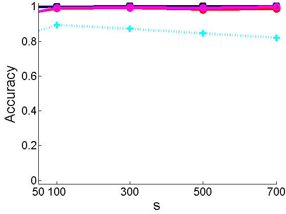
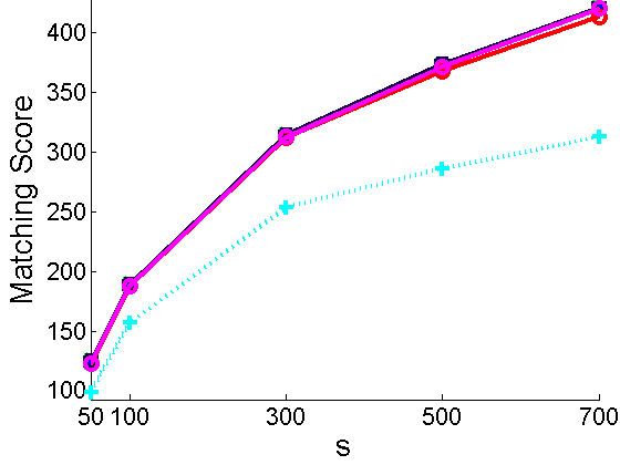
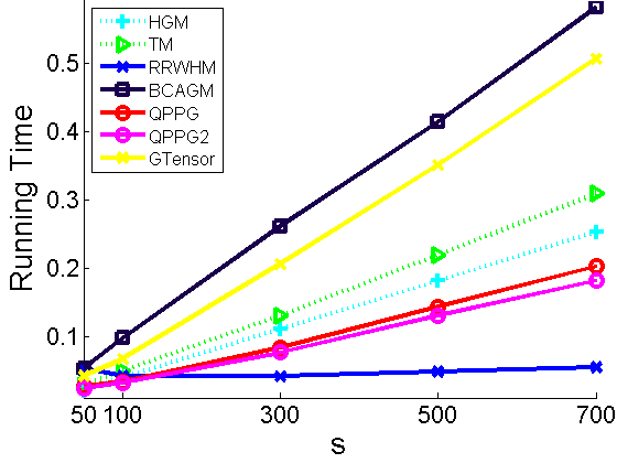
Figure 5.1: Results for different $s$.

Role of Upper Bound $M$. To see the role of $M$, numerical tests are performed on the synthetic data following the approach in duchenne2011tensor ; nguyen2016efficient . Firstly, $n_{1}$ points in $V_{1}$ are sampled following the standard normal distribution $\mathcal{N}(0,1)$. Secondly, points in $V_{2}$ are computed by $V_{2}=TV_{1}+\epsilon$, where $T\in\mathbb{R}^{n_{1}\times n_{1}}$ is a transformation matrix, and $\epsilon\in\mathbb{R}^{n_{1}}$ is the Gaussian noise. We choose $n_{1}=n_{2}$ ranging from 20 to 100, and $M$ from 1 to 10000. All experiments are executed for 100 times, and the average results are reported in Figure 5.2.

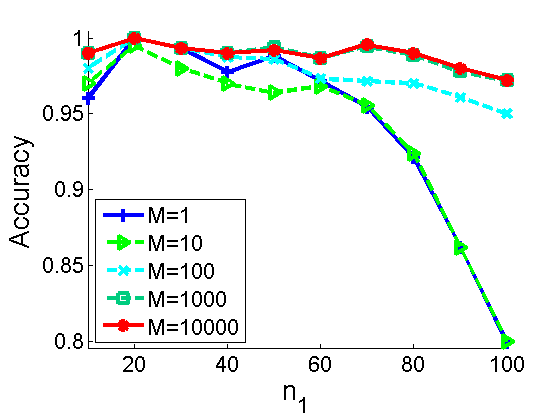
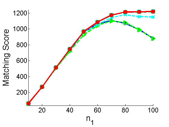
Figure 5.2: Results of QPPG for different $M$.

We can see that $M=1000$ or $M=10000$ produces competitive results, while $M\leq 100$ is not good for large problems in terms of both accuracy and CPU time. A possible reason is that small $M$ might lead to less flexibility for the entries in $x$. Hence, in the following results, we choose $M=10000$.

5.2 Performance of QPPG and QPPG2

In this subsection, we will illustrate the performance of our algorithm with synthetic data discussed above. We set $n_{1}=n_{2}=30$. Figure 5.3 shows the information while running Algorithm 2, including the accuracy, matching score and size of support set at $x^{k}$.

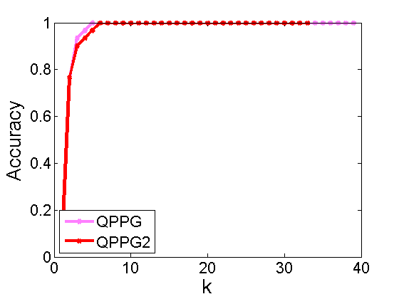
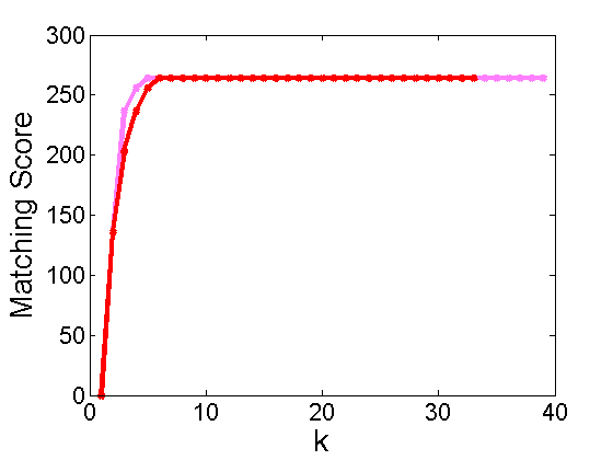
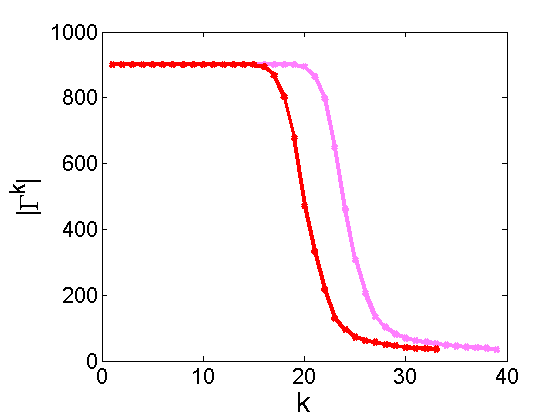
Figure 5.3: Accuracy, matching score and $|\Gamma^{k}|$ while running QPPG and QPPG2.

From Figure 5.3, one can find that $|\Gamma^{k}|$ keeps unchanged in the first few steps, and then drops rapidly from $n_{1}^{2}$ to $n_{1}$, while both accuracy and matching score reach their maximum value within five steps. It shows the potential of our algorithm for identifying the exact support set quickly, even during the process of iteration. This motivates us to stop our algorithm when $|\Gamma^{k}|$ is small enough, or stay unchanged for several iterations.

Figure 5.4: Entries in $x^{k}$ with $k=1,21,39$ by QPPG. The small circles in the bottom figure denote the true support set.

We also report the magnitude of entries in $x^{k}$ at several selected steps of QPPG in Figure 5.4. The algorithm stops at $k=39$. One can see that $|\Gamma^{k}|$ is decreasing. At the final step, the solution is sparse. This coincides with Remark 4, i.e., the magnitudes of the returned solution by our algorithm clearly fall into two parts: the estimated active part, which is usually close to zero, and the estimated nonzero part, which is the support set we are looking for.

5.3 CMU house dataset

In this subsection, we will test our algorithms on the CMU house dataset. Similar to Section 5.1, we try to match picture $v_{1}$ with $v_{2}$. As $v_{1}$ and $v_{2}$ change, we deal with different hypergraph matching test problems. For a fixed value $v=|v_{1}-v_{2}|$, we set $v_{1}=0,\ldots,110-v$ and $v_{2}=v,\ldots,110$. The total number of test examples is $111-v$. We test these examples, and plot the average results for each $v$ in Figure 5.5. One can see that most algorithms (except HGM) achieve good performance in terms of both accuracy and matching score. In terms of CPU time, QPPG and QPPG2 are competitive with HGM and TM, and faster than other methods.

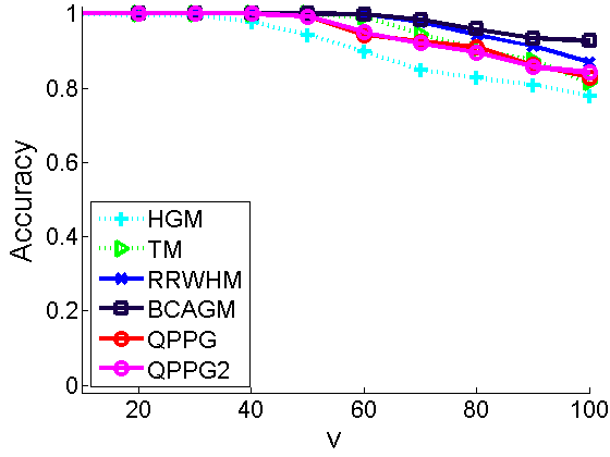
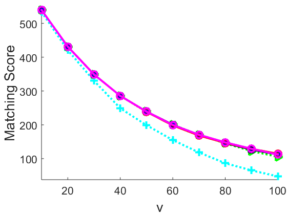
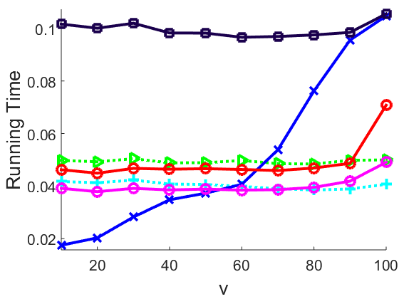
Figure 5.5: Results for CMU house dataset with $n_{1}=n_{2}=30$.

We also compare QPPG with other algorithms on CMU house dataset with $n_{1}=20$ and $n_{2}=30$. The results are obtained in a similar way as that for Figure 5.5, and are shown in Figure 5.6. One can see that QPPG performs well in both accuracy and matching score. As for CPU time, all the algorithms are competitive since the maximum time is about 0.06s. Figure 5.7 shows the matching results for two houses with $v_{1}=0$ and $v_{2}=60$.

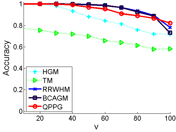
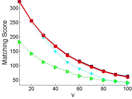
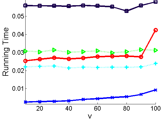
Figure 5.6: Results for CMU house dataset with $n_{1}=20$ and $n_{2}=30$.

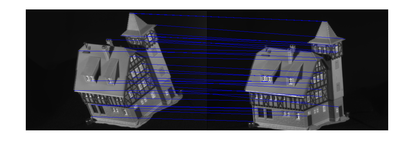
Figure 5.7: The matching results for two houses with $v_{1}=0$ and $v_{2}=60$ by QPPG. The blue lines are point-to-point correspondence.

5.4 Large dimensional synthetic data

In this section, large dimensional problems in the fish dataset are used to test our algorithms. We use all 100 examples in the subfolder res_fish_def_1. For each example, $V_{1}$ is the set of target fish, and $V_{2}$ is the set of deformation fish. The number of points in each set is around 100. Our task is to match the two sets. We select $n_{1}=n_{2}=10,20,\ldots,100$ points randomly from each fish (for fish with less than 100 points, we use all the points). The average results are shown in Figure 5.8. It can be seen that our algorithm is competitive with other methods in terms of accuracy, matching score and CPU time. One of the matching results is shown in Figure 5.9.

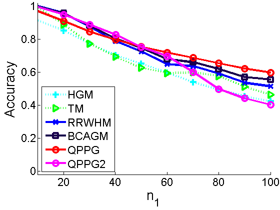
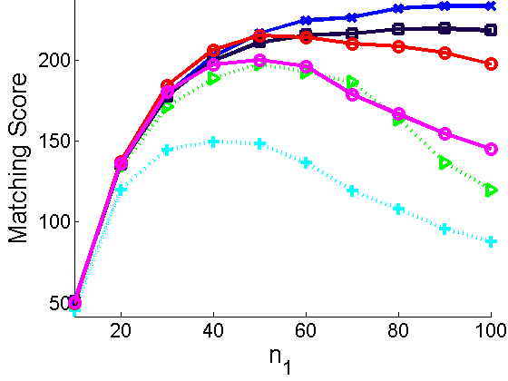
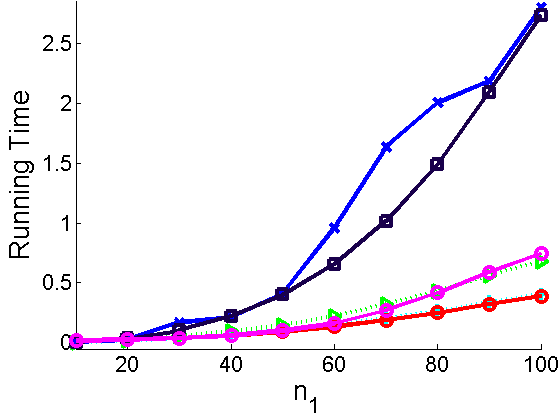
Figure 5.8: Results for the fish dataset.

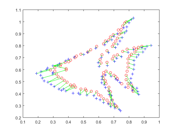
Figure 5.9: The matching results for fish dataset by QPPG. The red circles ‘$\circ$’ stand for points in $V_{1}$, and blue plus signs ‘$+$’ represent points in $V_{2}$. The green lines are point-to-point correspondence.

Furthermore, synthetic data explained in Section 5.1 is also used to test these algorithms. All the algorithms are tested except BCAGM, as their codes run into memory troubles for large-scale problems. We choose $n_{1}=n_{2}$ from 50 to 300, and repeat the tests for 100 times. The average results are reported in Figure 5.10. One can see that QPPG and QPPG2 perform comparably well with RRWHM in terms of both accuracy and matching score for $n_{1}$ less than or equal to 200. For $n_{1}$ greater than or equal to $250$, the running time for QPPG and QPPG2 increases slowly as $n_{1}$ increases, which implies that the proposed algorithm can deal with large-scale problems while returning good matching results.

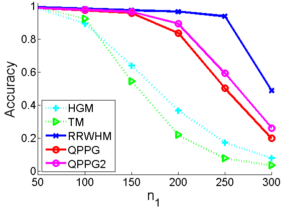
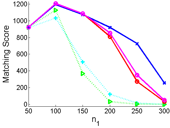
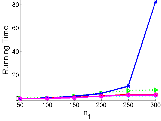
Figure 5.10: Results for synthetic data with large $n_{1}$.

6 Conclusions

In this paper, we reformulated hypergraph matching as a sparse constrained optimization problem. By dropping the sparse constraint, we showed that the relaxation problem has at least one global minimizer, which is also the global minimizer of the original problem. Aiming at seeking for the support set of the global minimizer of the original problem, we allowed violations of the equality constraints by penalizing them in a quadratic form. Then a quadratic penalty method was applied to solve the relaxation problem. Under reasonable assumptions, we showed that the support set of the global minimizer in hypergraph matching can be identified correctly without driving the penalty parameter to infinity. Numerical results demonstrated the high accuracy of the support set returned by our method.

References

- (1) Bauschke, H. H., Luke, D. R., Phan, H. M., and Wang, X.: Restricted normal cones and sparsity optimization with affine constraints. Found. Comput. Math. 14(1), 63–83 (2014)
- (2) Beck, A., and Eldar, Y. C.: Sparsity constrained nonlinear optimization: Optimality conditions and algorithms. SIAM J. Optim. 23(3), 1480–1509 (2013)
- (3) Berg, A. C., Berg, T. L., and Malik, J.: Shape matching and object recognition using low distortion correspondences. IEEE Conf. Computer Vision and Pattern Recognition 1, 26–33 (2005)
- (4) Bertsekas, D. P.: Projected newton methods for optimization problems with simple constraints. SIAM J. Control Optim. 20(2), 221–246 (1982)
- (5) Burdakov, O. P., Kanzow, C., and Schwartz, A.: Mathematical programs with cardinality constraints: Reformulation by complementarity-type conditions and a regularization method. SIAM J. Optim. 26(1), 397–425 (2016)
- (6) Calamai, P. H., and Moré, J. J.: Projected gradient methods for linearly constrained problems. Math. Program. 39(1), 93–116 (1987)
- (7) Cervinka, M., Kanzow, C., and Schwartz, A.: Constraint qualifications and optimality conditions for optimization problems with cardinality constraints. Math. Program. 160(1), 353–377 (2016)
- (8) Chen, X., Guo, L., Lu, Z., and Ye, J. J.: An augmented lagrangian method for non-lipschitz nonconvex programming. SIAM J. Numer. Anal. 55, 168–193 (2017)
- (9) Cui, C. F., Li, Q. N., Qi, L. Q. and Yan, H.: A quadratic penalty method for hypergraph matching. arXiv:1704.04581v1 (2017)
- (10) Dai, Y.-H., and Fletcher, R.: New algorithms for singly linearly constrained quadratic programs subject to lower and upper bounds. Math. Program. 106(3), 403–421 (2006)
- (11) Duchenne, O., Bach, F., Kweon, I.-S., and Ponce, J.: A tensor-based algorithm for high-order graph matching. IEEE Trans. Pattern Anal. Mach. Intell. 33(12), 2383–2395 (2011)
- (12) Egozi, A., Keller, Y., and Guterman, H.: A probabilistic approach to spectral graph matching. IEEE Trans. Pattern Anal. Mach. Intell. 35(1), 18–27 (2013)
- (13) Jiang, B., Liu, Y. F., and Wen, Z.: -norm regularization algorithms for optimization over permutation matrices. SIAM J. Optim. 26(4), 2284–2313 (2016)
- (14) Jiang, H., Drew, M. S., and Li, Z.-N.: Matching by linear programming and successive convexification. IEEE Trans. Pattern Anal. Mach. Intell. 29(6), 959–975 (2007)
- (15) Karp, Richard M.: Reducibility among combinatorial problems. Complexity of computer computations. springer US, 85–103 (1972)
- (16) Lee, J., Cho, M., and Lee, K. M.: Hyper-graph matching via reweighted random walks. IEEE Conf. Computer Vision and Pattern Recognition., 1633–1640 (2011)
- (17) Lee, J.-H., and Won, C.-H.: Topology preserving relaxation labelling for nonrigid point matching. IEEE Trans. Pattern Anal. Mach. Intell. 33(2), 427–432 (2011)
- (18) Li, X., and Song, W.: The first-order necessary conditions for sparsity constrained optimization. J. Oper. Res. Soc. China 3(4), 521–535 (2015)
- (19) Litman, R., and Bronstein, A. M.: Learning spectral descriptors for deformable shape correspondence. IEEE Trans. Pattern Anal. Mach. Intell. 36(1), 171–180 (2014)
- (20) Lu, Z., and Zhang, Y.: Sparse approximation via penalty decomposition methods. SIAM J. Optim. 23(4), 2448–2478 (2013)
- (21) Maciel, J., and Costeira, J. P.: A global solution to sparse correspondence problems. IEEE Trans. Pattern Anal. Mach. Intell. 25(2), 187–199 (2003)
- (22) Nguyen, Q., Tudisco, F., Gautier, A., and Hein, M.: An efficient multilinear optimization framework for hypergraph matching. IEEE Trans. Pattern Anal. Mach. Intell. 39(6), 1054-1075 (2017)
- (23) Nocedal, J., and Wright, S.: Numerical optimization. Springer Science & Business Media (2006)
- (24) Pan, L., Xiu, N., and Fan, J.: Optimality conditions for sparse nonlinear programming. Sci. China Math. 60(5), 759–776 (2017)
- (25) Pan, L., Xiu, N., and Zhou, S.: On solutions of sparsity constrained optimization. J. Oper. Res. Society of China 3(4), 421–439 (2015)
- (26) Pan, L., Zhou, S., Xiu, N., and Qi, H.: A convergent iterative hard thresholding for sparsity and nonnegativity constrained optimization. Pac. J. Optim. 13(2), 325-353 (2017)
- (27) Sun, W. Y., and Yuan, Y.-X.: Optimization theory and methods: nonlinear programming (Vol. 1). Springer Science & Business Media (2006)
- (28) Wu, M.-Y., Dai, D.-Q., and Yan, H.: Prl-dock: Protein-ligand docking based on hydrogen bond matching and probabilistic relaxation labeling. Proteins. Struct. Funct. Genet. 80(9), 2137–2153 (2012)
- (29) Yan, H.: Efficient matching and retrieval of gene expression time series data based on spectral information. Intern. Conf. Comput. Sci. Appl., 357–373 (2005)
- (30) Yan, J., Zhang, C., Zha, H., Liu, W., Yang, X., and Chu, S. M.: Discrete hyper-graph matching. IEEE Conf. Computer Vision and Pattern Recognition, 1520–1528 (2015)
- (31) Zaragoza, J., Chin, T.-J., Brown, M. S., and Suter, D.: As-projective-as-possible image stitching with moving DLT. IEEE Conf. Computer Vision and Pattern Recognition, 2339–2346 (2013)
- (32) Zaragoza, J., Chin, T.-J., Tran, Q.-H., Brown, M. S., and Suter, D.: As-projective-as-possible image stitching with moving DLT. IEEE Trans. Pattern Anal. Mach. Intell., 36(7), 1285–1298 (2014)
- (33) Zass, R., and Shashua, A.: Probabilistic graph and hypergraph matching. IEEE Conf. Computer Vision and Pattern Recognition, 1–8 (2008)
- (34) Zhou, J., Yan, H., and Zhu, Y.: Local topology preserved tensor models for graph matching. IEEE Conf. Syst. Man. Cybern., 2153–2157 (2015)