Weak quasielastic electroproduction of hyperons with polarization observables

Abstract

With the availability of high luminosity electron beam at the accelerators, there is now the possibility of studying weak quasielastic hyperon production off the proton, i.e. $e^{-}p\to\nu_{e}Y(Y=\varLambda,\varSigma^{0})$, which will enable the determination of the nucleon-hyperon vector and axial-vector transition form factors at high $Q^{2}$ in the strangeness sector and provide test of the Cabibbo model, G-invariance, CVC, PCAC hypotheses and SU(3) symmetry. In this work, we have studied the total cross section, differential cross section as well as the longitudinal and perpendicular components of polarization of the final hyperons ($\varLambda$ and $\varSigma^{0}$ produced in these reactions) and presented numerical results for these observables and their sensitivity to the transition form factors.

I Introduction

The study of weak interaction processes at high energy and momentum transfers is done with the experiments performed using neutrino and antineutrino beams. The interpretation of these experiments to understand the QCD structure of nucleons and extract various parameters of weak interaction phenomenology suffers from the systematic uncertainties arising due to the lack of well-understood (anti)neutrino flux and the nuclear medium effects due to the presence of heavy nuclear targets used in the large volume detectors. An extensive discussion of these systematic uncertainties and theoretical attempts to model them exists in the literature Katori:2016yel ; Morfin:2012kn ; Alvarez-Ruso:2014bla . The presence of these systematic uncertainties can be eliminated if the monoenergetic beams of the charged lepton probes can be used with the proton as the target to study the weak interaction processes.

The study of such processes has been proposed almost 50 years back but has not been seriously pursued due to the very small cross sections making it difficult to observe them experimentally Fearing:1969nr . Theoretically, there have been very few calculations to study the weak interaction processes induced by the electrons and they have been limited to the study of the quasielastic processes in the $\varDelta$S = 0 sector at very low energies from the nuclear targets relevant for the astrophysical applications Langanke:2002ab ; Suzuki:2011zzc . In the high energy region the study of weak inelastic excitations of $\varDelta$ and $N^{*}$ in the $\varDelta$S = 0 sector AlvarezRuso:1997jr ; Hwang:1987sd ; Nath:1979qe ; Pollock:1998tz ; Wang:2013kkc ; Wang:2014guo ; Jones:1979aj ; Mukhopadhyay:1998mn ; Hammer:1995dea and the quasielastic production of hyperons in the $|\varDelta$S$|$ = 1 sector induced by the electrons on the protons have been studied in the recent past Hwang:1988fp ; Mintz:2004eu ; Mintz:2002cj ; Mintz:2001jc .

It has been shown in these studies that with the availability of high luminosity unpolarized and polarized electron beams as well as the unpolarized and polarized proton targets there is the possibility of performing electron scattering experiments to study the weak processes in the charged and neutral current sectors at high energy and momentum transfers. Indeed, the polarized electrons have been used for the last many years to study the weak interaction processes which have been, however, limited to the neutral current sector. The study of the parity violating asymmetry in the scattering of polarized electrons from the proton targets has provided important information about the vector and axial-vector neutral current coupling of the electrons to the quarks in the DIS processes Prescott:1979dh ; Cahn:1977uu ; Brady:2011uy ; Matsui:2005ns ; Gorchtein:2011mz ; Hall:2013hta ; Mantry:2010ki ; Hobbs:2008mm and the $N-\varDelta$ transition form factors in the inelastic processes AlvarezRuso:1997jr ; Hwang:1987sd ; Nath:1979qe ; Pollock:1998tz ; Wang:2013kkc ; Wang:2014guo ; Jones:1979aj ; Mukhopadhyay:1998mn ; Hammer:1995dea as well as the presence of strangeness in the nucleon form factors in the quasielastic processes Musolf:1993tb ; GonzalezJimenez:2011fq ; Armstrong:2012bi ; Kumar:2013yoa ; Beise:2004py . However, no experimental attempts have been made to study the weak processes induced by the high energy electrons in the charge current sector.

With the luminosity of $10^{39}-10^{40}/\rm{cm}^{2}/\rm{s}$ of the electron beam which may be presently available at JLab Rode:2010zz ; jlab and MAMI mainz , it should be possible to study the weak production of $\varDelta$ and hyperons ($\varLambda$ and $\varSigma$).

Although the hyperon production is suppressed as compared to the $\varDelta$ production by a factor of $\rm{tan}^{2}\theta_{c}$ where $\theta_{c}$ is the Cabibbo angle, it could be important in the energy region close to the threshold of $\varDelta$ production where the $\varDelta$ production cross section is small due to the threshold effects. It would be, therefore, interesting to quantitatively study the kinematic region where the hyperon production becomes significant specially in the low energy region of electrons. At higher electron energies, the weak hyperon production is overwhelmed by the electromagnetic associated production of $\varLambda(\varSigma^{0})$, i.e. $e^{-}+p\longrightarrow e^{-}+\varLambda(\varSigma^{0})+K^{+}$, which happens at the electron energies above the energy corresponding to the threshold of associated particle production processes. However, the weak quasielastic production of $\varLambda$ is clearly distinguishable from the associated electroproduction of $\varLambda$ as it produces no electron in the final state but only the hadronic states of the nucleons and the pions through its decay products. Therefore, in this energy region the pion production without electrons is a clear signal of weak production of $\varLambda$ and $\varDelta$ in the final state. However, the electron induced weak production of pions can be seen even at lower energies corresponding to the threshold production of pions through the processes $e^{-}+p\longrightarrow\nu+n+\pi^{+}$ and $e^{-}+p\longrightarrow\nu+p+\pi^{0}$ which take place through the nonresonant processes mediated by pions and nucleons as well as the contact term required by the gauge invariance. As the energy increases, the nonresonant and the resonant production along with $\varLambda$ production contribute to the weak pion production. The low energy weak production of pions in the threshold region is an important topic in itself and provides valuable information about the electroweak multipoles Bernard:1993xh ; Ch . However, this has not been studied in the case of threshold weak pion production induced by electrons and is beyond the scope of the present work.

In the case of quasielastic reactions whenever the $\varLambda$ and $\varSigma^{0}$ hyperons are produced by the charged current interaction, the observation of the differential cross section and the polarization of final hyperons can yield important information about the nucleon-hyperon transition form factors and enable the study of the applicability of Cabibbo model, G-invariance, T-invariance and SU(3) symmetry at high $Q^{2}$ in the strangeness sector. This would extend our understanding of the weak interaction phenomenology in the strangeness sector to high $Q^{2}$ which is presently available only at very low $Q^{2}$ from the study of semileptonic decays of hyperons Cabibbo:2003cu ; Gaillard:1984ny ; Gazia . The observation of hyperons in the final state through its decay products, i.e. $\varLambda/\varSigma\longrightarrow N\pi$, and the structure of the angular distribution of pions will give information about the polarization of hyperons. The polarization observables of the hyperons produced in the quasielastic reactions induced by $\bar{\nu}_{\mu}$ are shown to be more sensitive to the weak axial form factors Erriquez:1978pg ; Alam:2014bya ; Alam:2013cra ; Pais:1971er ; Marshak ; LlewellynSmith:1971uhs ; Akbar:2016awk .

In view of the above discussion, we have studied in this paper the total cross section, differential cross section and the polarization observables of the final hyperons produced in

$$e^{-}+p\longrightarrow\varLambda(\varSigma^{0})+\nu_{e}$$ (1)

reactions and their sensitivity on the nucleon-hyperon transition form factors.

In section-II.1, the formalism to calculate the quasielastic weak hyperon production cross section and the expressions for the differential cross section $(\frac{d\sigma}{dQ^{2}})$, longitudinal ($P_{L}(Q^{2})$) and perpendicular ($P_{P}(Q^{2})$) components of the hyperon polarization are given. In section-II.2, we have given in brief the formalism to calculate the $\varDelta^{0}$ production cross section for the electron on the proton target. In section-III, we have presented the numerical results for the total cross section ($\sigma$), angular ($\frac{d\sigma}{d\Omega}$) and $Q^{2}$ ($\frac{d\sigma}{dQ^{2}}$) distributions and compared the results for the $Q^{2}$ distribution and $\sigma$ for the $\varLambda(\varSigma^{0})$ productions with the corresponding results for the $\varDelta^{0}$ production. We have presented the numerical results for the longitudinal $P_{L}(Q^{2})$ and perpendicular $P_{P}(Q^{2})$ polarization components of $\varLambda/\varSigma^{0}$ and discussed their sensitivity to the nucleon–hyperon transition from factors. All the numerical calculations have been performed in the lab frame, i.e., assuming the nucleon to be at rest. Our findings are summarized in section-IV.

II Formalism

II.1 $e^{-}~{}+~{}p\rightarrow\nu_{e}~{}+~{}Y$ process

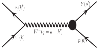
Figure 1: Feynman diagram for the process $e^{-}(k)+p(p)\rightarrow\nu_{e}(k^{\prime})+Y(p^{\prime})$, where $Y$ stands for final hyperon. The quantities in the bracket represent four momentum of the corresponding particles.

II.1.1 Cross section

The general expression of the differential cross section corresponding to the process presented in Fig. 1 may be written as

$$d\sigma=\frac{1}{(2\pi)^{2}}\frac{1}{4E_{e}^{L}m_{N}}\delta^{4}(k+p-k^{\prime}-p^{\prime})\frac{d^{3}k^{\prime}}{2E_{k^{\prime}}}\frac{d^{3}p^{\prime}}{2E_{p^{\prime}}}\overline{\sum}\sum|{\cal{M}}|^{2},$$ (2)

where $E_{e}^{L}$ is the electron energy in the lab frame and the square of the transition matrix element is defined in terms of the leptonic (${\cal L}_{\alpha\beta}$) and hadronic (${\cal J}^{\alpha\beta}$) tensors:

$$\overline{\sum}\sum|{\cal{M}}|^{2}=\frac{G_{F}^{2}\sin^{2}\theta_{c}}{2}\cal{J}^{\alpha\beta}\cal{L}_{\alpha\beta}.$$ (3)

In the above expression, $G_{F}$ is the Fermi coupling constant. The hadronic and leptonic tensors are given by

$$\cal{J}_{\alpha\beta} = \frac{1}{2}\mathrm{Tr}\left[\varLambda(p^{\prime})J_{\alpha}\varLambda(p)\tilde{J}_{\beta}\right]$$ (4)

$$\cal{L}^{\alpha\beta} = \frac{1}{2}\mathrm{Tr}\left[\gamma^{\alpha}(1-\gamma_{5})(k\!\!\!/+m_{e})\gamma^{\beta}(1-\gamma_{5})k^{\prime}\!\!\!\!\!/~{}\right],$$ (5)

with $\tilde{J}_{\beta}=\gamma^{0}J^{\dagger}_{\beta}\gamma^{0}$ and $\varLambda(p)=p\!\!\!/+m_{p}$.

$J_{\alpha}$ is the hadronic current operator given by

$$J_{\alpha}=V_{\alpha}-A_{\alpha},$$ (6)

where

$$V_{\alpha}=\gamma_{\alpha}f^{NY}_{1}(Q^{2})+i\sigma_{\alpha\beta}\frac{q^{\beta}}{m_{N}+m_{Y}}f^{NY}_{2}(Q^{2})+\frac{q_{\alpha}}{m_{N}+m_{Y}}f^{NY}_{3}(Q^{2}),$$ (7)

and

$$A_{\alpha}=\gamma_{\alpha}\gamma_{5}g^{NY}_{1}(Q^{2})+i\sigma_{\alpha\beta}\gamma_{5}\frac{q^{\beta}}{m_{N}+m_{Y}}g^{NY}_{2}(Q^{2})+\frac{q_{\alpha}}{m_{N}+m_{Y}}g^{NY}_{3}(Q^{2})\gamma_{5}.$$ (8)

$m_{N}$ and $m_{Y}$ are the masses of the initial and final baryons, and $q_{\mu}(=k_{\mu}-k_{\mu}^{\prime}=p_{\mu}^{\prime}-p_{\mu})$ is the four momentum transfer with $Q^{2}=-q^{2},~{}Q^{2}\geq 0$.

Using the above definitions, the $Q^{2}$ distribution is written as

$$\frac{d\sigma}{dQ^{2}}=\frac{1}{64\pi m_{N}^{2}{E_{e}^{L}}^{2}}\overline{\sum}\sum|{\cal{M}}|^{2}.$$ (9)

In Eq. (9), $|{\cal{M}}|^{2}$ is calculated using Eq. (3) assuming the absence of the second class currents and neglecting the contribution from the pseudoscalar term due to the small mass of the electron. The transition form factors $f^{NY}_{i}(Q^{2})$ and $g^{NY}_{i}(Q^{2})$ $(i=1-3)$, appearing in Eqs. (7) and (8), respectively, are determined using the conservation of vector current (CVC), the partial conservation of axial current (PCAC), the principles of T–invariance and G–invariance and the SU(3) symmetry.

II.1.2 Form Factors

The six form factors $f^{NY}_{i}(Q^{2})$ and $g^{NY}_{i}(Q^{2})$ ($i=1-3$) are determined using the following assumptions about the vector and axial vector currents in the weak interactions:

1. The assumption of the T–invariance implies that all the form factors $f^{NY}_{i}(Q^{2})$ and $g^{NY}_{i}(Q^{2})$ given in Eqs. (7) and (8), respectively, are real.

2. The assumption of the SU(3) symmetry of the weak hadronic currents implies that the vector and axial vector currents transform as an octet under the SU(3) group of transformations.

   Since the initial and final baryons also belong to the octet representation, therefore, each form factor $f^{NY}_{i}(Q^{2})$ ($g^{NY}_{i}(Q^{2})$) occurring in the matrix element of the vector (axial vector) current is written in terms of the two functions $D(Q^{2})$ and $F(Q^{2})$ corresponding to the symmetric octet($8^{S}$) and antisymmetric octet($8^{A}$) couplings of octets of vector (axial vector) currents. Specifically, we write

   $$f^{NY}_{i}(Q^{2})=aF_{i}^{V}(Q^{2})+bD_{i}^{V}(Q^{2}),$$ (10)

   $$g^{NY}_{i}(Q^{2})=aF_{i}^{A}(Q^{2})+bD_{i}^{A}(Q^{2}),$$ (11)

   where $a$ and $b$ are SU(3) Clebsch-Gordan coefficients given in Table-1. $F_{i}^{V,A}(Q^{2})$ and $D_{i}^{V,A}(Q^{2})$ are the couplings corresponding to the antisymmetric and symmetric couplings of the two octets.

3. For the determination of the vector form factors we have assumed the CVC and SU(3) symmetry which lead to $f^{NY}_{3}(Q^{2})=0$. Further, the remaining two vector form factors viz. $f^{NY}_{1}(Q^{2})$ and $f^{NY}_{2}(Q^{2})$ are determined in terms of the electromagnetic form factors of the nucleon, i.e. $f_{1}^{N}(Q^{2})$ and $f_{2}^{N}(Q^{2})$. This is done by taking the matrix element of the electromagnetic current operator between the nucleon states and determining $F_{i}^{V}(Q^{2})$ and $D_{i}^{V}(Q^{2})$ in terms of the electromagnetic form factors $f^{N}_{i}(Q^{2})$ $(i=1,2)$ of the nucleon. The functions $F_{i}^{V}(Q^{2})$ and $D_{i}^{V}(Q^{2}),\,(i=1,2)$ are thus expressed in terms of the nucleon form factors $f_{1}^{p,n}(Q^{2})$ and $f_{2}^{p,n}(Q^{2})$ as

   $$F_{i}^{V}(Q^{2}) = f_{i}^{p}(Q^{2})+\frac{1}{2}f_{i}^{n}(Q^{2}),$$ (12)

   $$D_{i}^{V}(Q^{2}) = -\frac{3}{2}f_{i}^{n}(Q^{2}).$$ (13)

   The vector form factors $f^{NY}_{i}(Q^{2}),i=1,2$ are derived using Eq. (10) and are tabulated in Table-2.

4. In the axial vector sector, the form factor $g^{NY}_{2}(Q^{2})$ vanishes due to G–invariance, T–invariance and SU(3) symmetry. The axial vector form factor $g^{NY}_{1}(Q^{2})$ is determined from Eq. (11). We write the axial vector form factor $g^{NY}_{1}(Q^{2})$ in terms of two functions $F_{1}^{A}(Q^{2})$ and $D_{1}^{A}(Q^{2})$. Using Table-1 for the coefficients $a$ and $b$, we find

   $$g_{1}^{p\varLambda}(Q^{2}) = \sqrt{\frac{1}{6}}\left(3F^{A}_{1}(Q^{2})+D^{A}_{1}(Q^{2})\right),$$

   $$g_{1}^{p\varSigma^{0}}(Q^{2}) = \sqrt{\frac{1}{2}}\left[D^{A}_{1}(Q^{2})-F^{A}_{1}(Q^{2})\right],$$ (14)

   which are rewritten in terms of the axial vector form factor $g_{A}^{np}(Q^{2})(=F_{1}^{A}(Q^{2})+D_{1}^{A}(Q^{2}))$ for the $n-p$ transition and are given in Table-2 with $x(Q^{2})$ defined as

   $$x(Q^{2})=\frac{F^{A}_{1}(Q^{2})}{F^{A}_{1}(Q^{2})+D^{A}_{1}(Q^{2})}.$$ (15)

   We further assume that $F^{A}_{1}(Q^{2})$ and $D^{A}_{1}(Q^{2})$ have the same $Q^{2}$ dependence, such that $x(Q^{2})$ becomes a constant and is given by $x=\frac{F^{A}_{1}(0)}{F^{A}_{1}(0)+D_{1}^{A}(0)}$. For $g_{A}^{np}(Q^{2})$, a dipole parameterization has been used

   $$g_{A}^{np}(Q^{2})=g_{A}(0)\left(1+\frac{Q^{2}}{M_{A}^{2}}\right)^{-2},$$ (16)

   where $M_{A}$ is the axial dipole mass and for the numerical calculations we have used $M_{A}=1.026$ GeV Bernard:2001rs . The axial charge $g_{A}(0)=1.2723$ and $x=0.364$ Cabibbo:2003cu are determined from the experimental data on the $\beta$ decay of neutron and the semileptonic decay of hyperons.

	$p\to\varLambda$	$p\to\varSigma^{0}$	$p\to n$
$a$	$-\sqrt{\frac{3}{2}}$	$-\frac{1}{\sqrt{2}}$	1
$b$	$-\sqrt{\frac{1}{6}}$	$\frac{1}{\sqrt{2}}$	1

Table 1: Values of the coefficients $a$ and $b$ given in Eqs. (10) and (11).

$e^{-}p\rightarrow\nu_{e}\varLambda$ $e^{-}p\rightarrow\nu_{e}\varSigma^{0}$ $f_{1}^{NY}(Q^{2})$ $-\sqrt{\frac{3}{2}}~{}f_{1}^{p}(Q^{2})$ $-\frac{1}{\sqrt{2}}\left[f_{1}^{p}(Q^{2})+2f_{1}^{n}(Q^{2})\right]$ $f_{2}^{NY}(Q^{2})$ $-\sqrt{\frac{3}{2}}~{}f_{2}^{p}(Q^{2})$ $-\frac{1}{\sqrt{2}}\left[f_{2}^{p}(Q^{2})+2f_{2}^{n}(Q^{2})\right]$ $g_{1}^{NY}(Q^{2})$ $-\frac{1}{\sqrt{6}}(1+2x)g_{A}(Q^{2})$ $\frac{1}{\sqrt{2}}(1-2x)g_{A}(Q^{2})$

Table 2: Vector and axial vector from factors for $e^{-}(k)+p(p)\rightarrow\nu_{e}(k^{\prime})+Y(p^{\prime})$ processes.

II.1.3 Polarization of hyperons

Using the covariant density matrix formalism, the polarization 4-vector($\xi^{\tau}$) of the final hyperon produced in reaction (1) is written as Bilekny

$$\xi^{\tau}=\frac{\mathrm{Tr}[\gamma^{\tau}\gamma_{5}~{}\rho_{f}(p^{\prime})]}{\mathrm{Tr}[\rho_{f}(p^{\prime})]},$$ (17)

where the final spin density matrix $\rho_{f}(p^{\prime})$ is given by

$$\rho_{f}(p^{\prime})={\cal L}^{\alpha\beta}\varLambda(p^{\prime})J_{\alpha}\varLambda(p)\tilde{J}_{\beta}\varLambda(p^{\prime}).$$ (18)

Using the following relations Bilenky:2013fra ; Bilenky:2013iua :

$$\varLambda(p^{\prime})\gamma^{\tau}\gamma_{5}\varLambda(p^{\prime})=2m_{Y}\left(g^{\tau\sigma}-\frac{p^{\prime\tau}p^{\prime\sigma}}{m_{Y}^{2}}\right)\varLambda(p^{\prime})\gamma_{\sigma}\gamma_{5}$$ (19)

and

$$\varLambda(p^{\prime})\varLambda(p^{\prime})=2m_{Y}\varLambda(p^{\prime}),$$ (20)

$\xi^{\tau}$ defined in Eq. (17) may be rewritten as

$$\xi^{\tau}=\left(g^{\tau\sigma}-\frac{p^{\prime\tau}p^{\prime\sigma}}{m_{Y}^{2}}\right)\frac{{\cal L}^{\alpha\beta}\mathrm{Tr}\left[\gamma_{\sigma}\gamma_{5}\varLambda(p^{\prime})J_{\alpha}\varLambda(p)\tilde{J}_{\beta}\right]}{{\cal L}^{\alpha\beta}\mathrm{Tr}\left[\varLambda(p^{\prime})J_{\alpha}\varLambda(p)\tilde{J}_{\beta}\right]}.$$ (21)

Note that in Eq. (21), $\xi^{\tau}$ is manifestly orthogonal to $p^{\prime\tau}$, i.e. $p^{\prime}\cdot\xi=0$. Moreover, the denominator is directly related to the differential cross section given in Eq. (9).

With ${\cal J}^{\alpha\beta}$ and ${\cal L}_{\alpha\beta}$ given in Eqs. (4) and (5), respectively, an expression for $\xi^{\tau}$ is obtained. In the lab frame where the initial nucleon is at rest, the polarization vector $\bm{\xi}$ is calculated to be a function of 3-momenta of incoming electron $(\textbf{{k}})$ and outgoing hyperon $(\textit{{p}}^{\prime})$, and is given as

$$\bm{\xi}=\left[{\bm{k}}~{}\alpha(Q^{2})+{\bm{p}}\,^{\prime}\beta(Q^{2})\right],$$ (22)

where the expressions of $\alpha(Q^{2})$ and $\beta(Q^{2})$ are given in the appendix.

From Eq. (22), it follows that the polarization vector lies in the scattering plane defined by ${\bm{k}}$ and $\bm{p}\,^{\prime}$, and there is no component of polarization in a direction orthogonal to the scattering plane. This is a consequence of T–invariance which makes the transverse polarization in a direction perpendicular to the reaction plane vanish Pais:1971er ; LlewellynSmith:1971uhs . We now expand the polarization vector $\bm{\xi}$ along the two orthogonal directions, ${\bm{e}}_{L}$ and ${\bm{e}}_{P}$ in the reaction plane corresponding to the longitudinal and perpendicular directions, to the momentum of hyperon i.e.

$$\bm{e}_{L}=\frac{\bm{p^{\prime}}}{|\bm{p^{\prime}}|},\qquad\bm{e}_{P}=\bm{e}_{L}\times\bm{e}_{T},\qquad{\rm where}~{}~{}~{}~{}~{}\bm{e}_{T}=\frac{\bm{p^{\prime}}\times\bm{k}}{|\bm{p^{\prime}}\times\bm{k}|},$$ (23)

and write

$$\bm{\xi}=\xi_{P}\bm{e}_{P}+\xi_{L}\bm{e}_{L},$$ (24)

such that the longitudinal and perpendicular components of the polarization vector ($\bm{\xi}$) in the lab frame are given by

$$\xi_{L}(Q^{2})=\bm{\xi}\cdot\bm{e}_{L},\qquad\xi_{P}(Q^{2})=\bm{\xi}\cdot\bm{e}_{P}.$$ (25)

From Eq. (25), the longitudinal $P_{L}(Q^{2})$ and perpendicular $P_{P}(Q^{2})$ components of the polarization vector defined in the rest frame of the initial nucleon are given by  Bilenky:2013fra ; Bilenky:2013iua

$$P_{L}(Q^{2})=\frac{m_{Y}}{E_{p^{\prime}}}\xi_{L}(Q^{2}),\qquad P_{P}(Q^{2})=\xi_{P}(Q^{2}),$$ (26)

where $\frac{m_{Y}}{E_{p^{\prime}}}$ is the Lorentz boost factor along ${\bm{p}}^{\prime}$. With the help of Eqs. (22), (23), (25) and (26), the longitudinal component $P_{L}(Q^{2})$ is calculated to be

$$P_{L}(Q^{2})=\frac{m_{Y}}{E_{p^{\prime}}}\left(\frac{\alpha(Q^{2}){\bm{k}}\cdot{\bm{p}}\,^{\prime}+\beta(Q^{2})|{\bm{p}}\,^{\prime}|^{2}}{|{\bm{p}}\,^{\prime}|~{}{\cal J}^{\alpha\beta}{\cal L}_{\alpha\beta}}\right),$$ (27)

where $E_{p^{\prime}}=\sqrt{|{{\bm{p}}^{\prime}}|^{2}+m_{Y}^{2}}$. Similarly, the perpendicular component $P_{P}(Q^{2})$ of the polarization 3-vector is given as

$$P_{P}(Q^{2})=\frac{({\bm{k}}\cdot{\bm{p}^{\prime}})^{2}-|{\bm{k}}|^{2}|{\bm{p}}\,^{\prime}|^{2}}{|{\bm{p}}\,^{\prime}||{\bm{p^{\prime}}}\times{\bm{k}}|~{}{\cal J}^{\alpha\beta}{\cal L}_{\alpha\beta}}\alpha(Q^{2}).$$ (28)

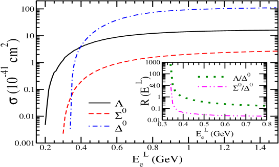
Figure 2: $\sigma$ vs. $E_{e}^{L}$ for $\varLambda$ (solid line), $\varSigma^{0}$ (dashed line) and $\varDelta^{0}$ (dashed-dotted line) productions. In the inset the results are presented for the ratio $R(E_{e}^{L})=\frac{\sigma_{Y}}{\sigma_{\varDelta^{0}}}$ vs. $E_{e}^{L}$, for Y=$\varLambda$ (dotted line), $\varSigma^{0}$ (dashed double-dotted line).

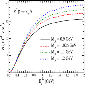
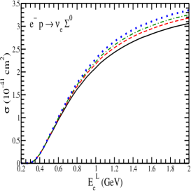
Figure 3: $\sigma$ vs. $E_{e}^{L}$ for $e^{-}p\to\nu_{e}\varLambda$ (left panel) and $e^{-}p\to\nu_{e}\varSigma^{0}$ (right panel) processes. The results are presented for different values of $M_{A}$ viz. 0.9 GeV (solid line), 1.026 GeV (dashed line), 1.1 GeV (dash-dotted line) and 1.2 GeV (dotted line).

II.2 $e^{-}~{}+~{}p\rightarrow\nu_{e}~{}+~{}\varDelta^{0}$ process

In order to compare the cross section for the hyperon production with the cross section for the $\varDelta^{0}$ production, produced in the reaction

$$e^{-}(k)~{}+~{}p(p)\rightarrow\nu_{e}(k^{\prime})~{}+~{}\varDelta^{0}(p^{\prime}),$$ (29)

we give the expression for the differential cross section for the $\varDelta^{0}$ production as AlvarezRuso:1997jr

$$\frac{d\sigma}{dQ^{2}}=\frac{1}{16\pi^{2}}\int{d|{\bm{p^{\prime}}}|}\frac{{|{{\bm{p}}^{\prime}}|}}{E_{e}^{2}E_{\nu_{e}}}\frac{\frac{\varGamma_{\varDelta}(W)}{2}}{(W-M_{\varDelta})^{2}+\frac{\varGamma_{\varDelta}^{2}(W)}{4}}\overline{\sum}\sum|{\cal{M}}|^{2}.$$ (30)

In the above expression $\overline{\sum}\sum|{\cal{M}}|^{2}=\frac{G_{F}^{2}}{2}\cos^{2}\theta_{c}\,\cal{L}_{\mu\nu}$ $J^{\mu\nu}$, where the leptonic tensor $\cal{L}_{\mu\nu}$ is given in Eq. (5) and the hadronic tensor $J^{\mu\nu}=\frac{1}{2}Tr\left[\frac{(\not p+m_{N})}{2m_{N}}{\tilde{\mathcal{O}}}^{\alpha\mu}{\it P}_{\alpha\beta}{\mathcal{O}}^{\beta\nu}\right]$. The hadronic tensor is obtained by using the expression for the hadronic current $j^{\mu}$ as

$$<\varDelta(p^{\prime})|j^{\mu}|p(p)>=\bar{\Psi}_{\beta}(p^{\prime}){\mathcal{O}}^{\beta\mu}u(p).$$ (31)

In the above expression $u(p)$ is the Dirac spinor for the proton and $\Psi_{\beta}$ is a Rarita-Schwinger field for spin-$\frac{3}{2}$ particle. $\mathcal{O}^{\beta\alpha}$ is the $N-\varDelta$ transition vertex, which is described in terms of the vector($C_{i}^{V}(q^{2})$) and the axial vector($C_{i}^{A}(q^{2})$) transition form factors with $\mathcal{O}^{\beta\alpha}={\mathcal{O}}_{V}^{\beta\alpha}+{\mathcal{O}}_{A}^{\beta\alpha}$, which are given by

$${\mathcal{O}}_{V}^{\beta\alpha}=\left(\frac{C_{3}^{V}(q^{2})}{m_{N}}(g^{\alpha\beta}\not\!q-q^{\beta}\gamma^{\alpha})+\frac{C_{4}^{V}(q^{2})}{m_{N}^{2}}(g^{\alpha\beta}q\cdot p^{\prime}-q^{\beta}p^{\prime\alpha})+\frac{C_{5}^{V}(q^{2})}{m_{N}^{2}}(g^{\alpha\beta}q\cdot p-q^{\beta}p^{\alpha})\right)\gamma_{5}$$ (32)

and

$${\mathcal{O}}_{A}^{\beta\alpha}=\left(\frac{C_{4}^{A}(q^{2})}{m_{N}}(g^{\alpha\beta}{\not\!q}-q^{\beta}\gamma^{\alpha})+C_{5}^{A}(q^{2})g^{\alpha\beta}+\frac{C_{6}^{A}(q^{2})}{m_{N}^{2}}q^{\beta}q^{\alpha}\right).$$ (33)

For the numerical calculations, we have taken the parameterization of Lalakulich et al. Lalakulich:2006sw for $C_{i}^{V}(Q^{2})$ and $C_{i}^{A}(Q^{2})$:

$$C_{i}^{V}(Q^{2})=C_{i}^{V}(0)~{}\left(1+\frac{Q^{2}}{M_{V}^{2}}\right)^{-2}~{}{\cal{D}}_{i},~{}~{}~{}i=3,4,5,$$ (34)

with $C_{3}^{V}(0)=2.13$, $C_{4}^{V}(0)=-1.51$ and $C_{5}^{V}(0)=0.48$,

$${\cal{D}}_{3,4} = \left(1+\frac{Q^{2}}{4M_{V}^{2}}\right)^{-1}~{}~{}~{}\mbox{and}$$

$${\cal{D}}_{5} = \left(1+\frac{Q^{2}}{0.776M_{V}^{2}}\right)^{-1};~{}~{}M_{V}=0.84~{}\rm{GeV}$$ (35)

and

$$C_{i}^{A}(Q^{2}) = C_{i}^{A}(0)\left(1+\frac{Q^{2}}{M_{A}^{2}}\right)^{-2}\left(1+\frac{Q^{2}}{3M_{A}^{2}}\right)^{-1};$$

$$M_{A} = 1.026~{}\rm{GeV}$$ (36)

for $i=3,4,5,6$ with $C_{3}^{A}(0)=0$, $C_{4}^{A}(0)=-0.25~{}C_{5}^{A}(0)$, $C_{5}^{A}(0)=-1.2$ and $C_{6}^{A}(0)=\frac{m_{N}^{2}}{(m^{2}_{\pi}+Q^{2})}C_{5}^{A}(0)$.

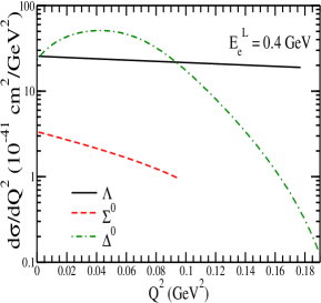
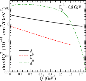
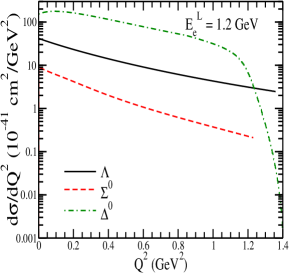
Figure 4: $\frac{d\sigma}{dQ^{2}}$ vs. $Q^{2}$ at $E_{e}^{L}$ = 0.4 GeV (left panel), $E_{e}^{L}$ = 0.8 GeV (central panel) and $E_{e}^{L}$ = 1.2 GeV (right panel). The results are shown for $\varLambda$ (solid line), $\varSigma^{0}$ (dashed line) and $\varDelta^{0}$ (dash-dotted line) productions.

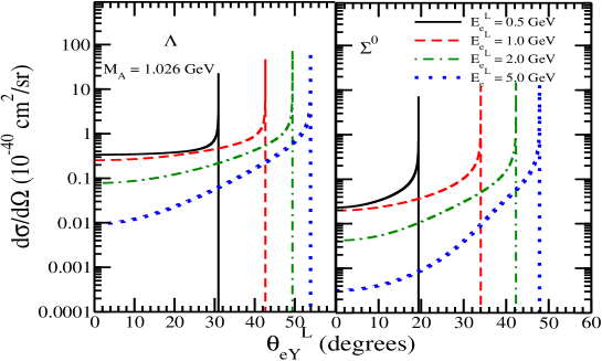
Figure 5: Hyperon angular distribution ($\frac{d\sigma}{d\Omega}$) vs. outgoing $Y$ laboratory angle ($\theta_{eY}^{L}$) for the processes $e^{-}p\to\nu_{e}\varLambda$ (left panel) and $e^{-}p\to\nu_{e}\varSigma^{0}$ (right panel) with $M_{A}$=1.026 GeV at different electron energies $E_{e}^{L}$= 0.5 GeV (solid line), 1 GeV (dashed line), 2 GeV (dash-dotted line) and 5 GeV (dotted line).

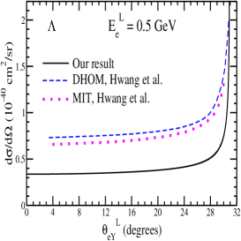
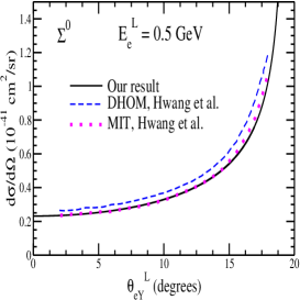
Figure 6: Hyperon angular distribution ($\frac{d\sigma}{d\Omega}$) vs. outgoing $Y$ laboratory angle ($\theta_{eY}^{L}$) for the processes $e^{-}p\to\nu_{e}\varLambda$ (left panel) and $e^{-}p\to\nu_{e}\varSigma^{0}$ (right panel) at $E_{e}^{L}$ = 0.5 GeV with $M_{A}=$ 1.026 GeV (solid line). The results are compared with the results obtained by Hwang et al. Hwang:1988fp using two different models, DHOM (dashed line) and MIT model (dotted line).

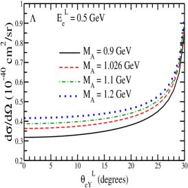
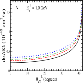
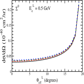
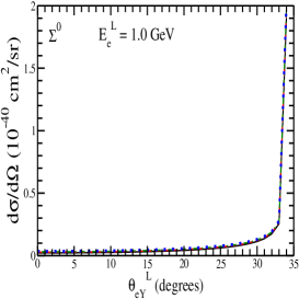
Figure 7: $\frac{d\sigma}{d\Omega}$ vs. outgoing $\theta_{eY}^{L}$ for the processes $e^{-}p\to\nu_{e}\varLambda$ (upper panel) and $e^{-}p\to\nu_{e}\varSigma^{0}$ (lower panel) at $E_{e}^{L}$ = 0.5 GeV (left panel), $E_{e}^{L}$ = 1 GeV (right panel). The results are presented for different values of $M_{A}$ viz. 0.9 GeV (solid line), 1.026 GeV (dashed line), 1.1 GeV (dash-dotted line) and 1.2 GeV (dotted line).

${\it P}_{\alpha\beta}$ is the spin-3/2 projection operator given by

$${\it P}_{\alpha\beta}=-(\frac{\not\!p^{\prime}+M_{\varDelta}}{2M_{\varDelta}})\left(g_{\alpha\beta}-\frac{2}{3}\frac{{p^{\prime}}_{\alpha}{p^{\prime}}_{\beta}}{M_{\varDelta}^{2}}+\frac{1}{3}\frac{{p^{\prime}}_{\alpha}\gamma_{\beta}-{p^{\prime}}_{\alpha}\gamma_{\beta}}{M_{\varDelta}}-\frac{1}{3}\gamma_{\alpha}\gamma_{\beta}\right),$$ (37)

and the delta decay width $\varGamma$ is taken as the energy dependent $P$-wave decay width given by

$$\varGamma_{\varDelta}(W)=\frac{1}{6\pi}\left(\frac{f_{\pi N\varDelta}}{m_{\pi}}\right)^{2}\frac{M_{\varDelta}}{W}|\bm{q}_{cm}|^{3},$$ (38)

where the $N-\varDelta$ coupling constant $f_{\pi N\varDelta}=2.127$, $m_{\pi}$ is the pion mass, $|\bm{q}_{cm}|$ is the pion momentum in the rest frame of the resonance and is given by

$$|{\bm{q}_{cm}}|=\frac{\sqrt{(W^{2}-m_{\pi}^{2}-M_{N}^{2})^{2}-4m_{\pi}^{2}M_{N}^{2}}}{2W},$$

with W [$(m_{N}+m_{\pi})\leq W<1.4~{}\rm{GeV}$] as the center-of-mass energy.

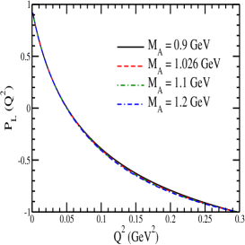
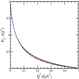
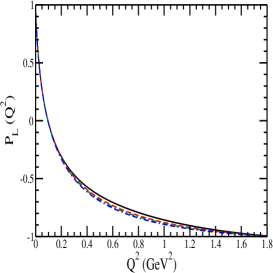
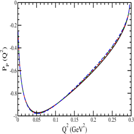
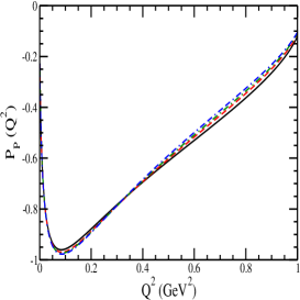
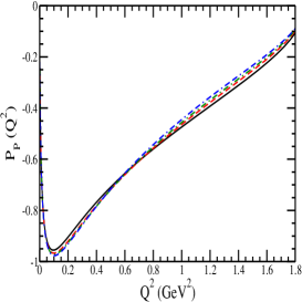
Figure 8: $P_{L}(Q^{2})$ and $P_{P}(Q^{2})$ vs. $Q^{2}$ for the process $e^{-}p\to\nu_{e}\varLambda$ at $E_{e}^{L}$ = 0.5 GeV (left panel), $E_{e}^{L}$ = 1 GeV (central panel) and $E_{e}^{L}$ = 1.5 GeV (right panel). The results are presented for different values of $M_{A}$ viz. 0.9 GeV (solid line), 1.026 GeV (dashed line), 1.1 GeV (dash-dotted line) and 1.2 GeV (dash–double-dotted line).

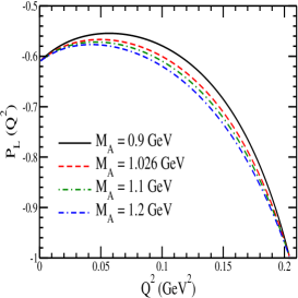
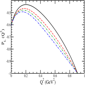
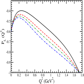
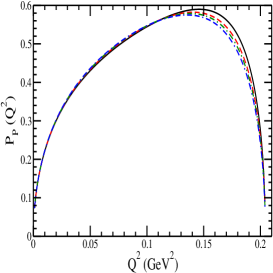
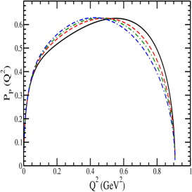
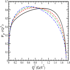
Figure 9: $P_{L}(Q^{2})$ and $P_{P}(Q^{2})$ vs. $Q^{2}$ for the process $e^{-}p\to\nu_{e}\varSigma^{0}$ at $E_{e}^{L}$ = 0.5 GeV (left panel), $E_{e}^{L}$ = 1 GeV (central panel) and $E_{e}^{L}$ = 1.5 GeV (right panel). The results are presented for different values of $M_{A}$ viz. 0.9 GeV (solid line), 1.026 GeV (dashed line), 1.1 GeV (dash-dotted line) and 1.2 GeV (dash–double-dotted line).

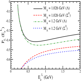
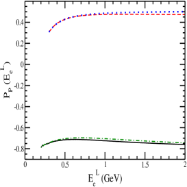
Figure 10: The results are presented for $P_{L}(E_{e}^{L})$ (left panel) and $P_{P}(E_{e}^{L})$ (right panel) vs. $E_{e}^{L}$ using Eq. (39) for the process $e^{-}p\to\nu_{e}\varLambda$ at $M_{A}$ = 1.026 GeV (solid line) and 1.2 GeV (dash-dotted line), and for $e^{-}p\to\nu_{e}\varSigma^{0}$ at $M_{A}$ = 1.026 GeV (dashed line) and 1.2 GeV (dotted line).

III Results and discussion

We have used Eq. (2) for the calculation of the total cross section $\sigma(E_{e}^{L})$ and the differential cross sections ($\frac{d\sigma}{dQ^{2}}$ and $\frac{d\sigma}{d\Omega}$), and Eqs. (27) and (28) for the longitudinal $P_{L}(Q^{2})$ and perpendicular $P_{P}(Q^{2})$ components of polarization, respectively, for the processes $e^{-}p\to\nu_{e}\varLambda$ and $e^{-}p\to\nu_{e}\varSigma^{0}$. The form factors are given in Table-2. For the vector nucleon form factors, we have used the parameterization of Bradford et al. Bradford:2006yz . A dipole parameterization for the nucleon axial vector form factor with the dipole mass $M_{A}=1.026$ GeV Bernard:2001rs has been used. For the $\varDelta^{0}$ production cross section, we have used Eq. (30) with the form factors defined in Eqs. (34) –(II.2) and integrated over the angles to get the total cross section ($\sigma(\varDelta)$).

In Fig. 2, we have presented the results of $\sigma$ vs. $E_{e}^{L}$ for $\varLambda$, $\varSigma^{0}$ and $\varDelta^{0}$ productions. In the inset of Fig. 2, we have also presented the results for the ratio $R(E_{e}^{L})=\frac{\sigma_{Y}}{\sigma_{\varDelta^{0}}}$, for Y = $\varLambda$ and $\varSigma^{0}$ productions. We observe that for energies $E_{e}^{L}~{}<~{}$0.4 GeV, the $\varLambda$ production cross section is more than the $\varDelta^{0}$ production which reduces to $\sim 24\%$ of the $\varDelta^{0}$ production for $E_{e}^{L}~{}\sim~{}$0.6 GeV and $\sim$ 16$\%$ for $E_{e}^{L}=$ 1 GeV. Thus, in the low electron energy range, the hyperons ($\varLambda,\varSigma^{0}$) give considerable contribution to the total cross section along with the $\varDelta^{0}$ production process. The hyperon and $\varDelta^{0}$ produced in these reactions decay to pion and nucleon. These particles may be observed in coincidence. With the availability of the high luminosity electron beam (say 10³⁹/cm²/s), we may be able to observe $\sim$ 665 events for the $\varDelta^{0}$ production and $\sim$ 248 and 20 events for $\varLambda$ and $\varSigma^{0}$ productions in the duration of 1 hour for 0.5 GeV electron energy, while almost the same number of events $\sim$ 150 for $\varLambda$ and $\varDelta^{0}$ productions at $E_{e}^{L}~{}=~{}$0.4 GeV.

To see the dependence of $\sigma$ on the axial dipole mass $M_{A}$, in Fig. 3, we have shown the results with $M_{A}$=0.9, 1.026, 1.1 and 1.2 GeV Wilkinson:2016wmz ; Ankowski:2016bji ; Stowell:2016exm . We find that the $\varLambda$ production cross section has larger sensitivity to $M_{A}$ than the $\varSigma^{0}$ production cross section. It should be possible to determine the value of $M_{A}$ in the strangeness sector by observing the total $\varLambda$ production in the energy range of 0.8$<E_{e}^{L}<$2 GeV.

In Fig. 4, we have presented the results for $\frac{d\sigma}{dQ^{2}}$ vs. $Q^{2}$ at different values of the electron energies viz. $E_{e}^{L}$=0.4, 0.8 and 1.2 GeV, for $\varLambda$, $\varSigma^{0}$ and $\varDelta^{0}$ productions. In the threshold region, at very low $Q^{2}$, there is almost equal contribution from the $\varLambda$ and $\varDelta^{0}$ productions. For $Q^{2}>$ 0.1 GeV² there is a sharp fall in the $\varDelta^{0}$ production cross section, whereas the $\varLambda$ production cross section decreases slowly, similar to $e^{-}p\to\nu_{e}n$ reaction. At $E_{e}^{L}=$ 0.8 GeV, the $\varLambda$ cross section is $\sim$ 10–30 $\%$ of the $\varDelta^{0}$ cross section in the low $Q^{2}$ region.

In Fig. 5, we have presented the results for the angular distribution $\frac{d\sigma}{d\Omega}$ for $\varLambda$ and $\varSigma^{0}$ in $e^{-}p\to\nu_{e}\varLambda$ and $e^{-}p\to\nu_{e}\varSigma^{0}$ reactions at different electron energies $E_{e}^{L}$=0.5, 1, 2 and 5 GeV. In general, the nature of the angular distribution is qualitatively similar at these energies. However, the peak shifts towards the smaller angles at lower $E_{e}^{L}$. We find that (not shown here) for $e^{-}p\to\nu_{e}\varLambda$ process, the major contribution to the cross section comes from $g_{1}^{2}(Q^{2})$ and $f_{1}^{2}(Q^{2})$ terms. Quantitatively, the contribution of $g_{1}^{2}(Q^{2})$ is larger at the smaller angles while the contribution from $f_{1}^{2}(Q^{2})$ is larger in the peak region. The contributions of the interference terms like $f_{1}(Q^{2})g_{1}(Q^{2})$ and $f_{2}(Q^{2})g_{1}(Q^{2})$ are almost of the same strength. The contribution from the $f_{1}(Q^{2})f_{2}(Q^{2})$ term is almost of equal strength at the smaller angles but becomes almost an order of magnitude smaller in the peak region as compared to the contribution of the vector-axial vector interference terms. For the process $e^{-}p\to\nu_{e}\varSigma^{0}$, it is the $f_{2}^{2}(Q^{2})$ term which dominates at the smaller angles followed by the $g_{1}^{2}(Q^{2})$ and $f_{1}^{2}(Q^{2})$ terms. However, in the peak region, the $f_{1}^{2}(Q^{2})$ term dominates followed by the $f_{2}^{2}(Q^{2})$ and $g_{1}^{2}(Q^{2})$ terms. The term $f_{2}(Q^{2})g_{1}(Q^{2})$ is the dominant interference term. We also find that there is not much effect of different parameterizations for the vector nucleon form factors $f^{p,n}_{1,2}$ available in the literature on the angular distribution for both $\varLambda$ and $\varSigma^{0}$. The present results are in agreement with the results of Mintz and collaborators Mintz:2004eu ; Mintz:2002cj ; Mintz:2001jc .

The angular distribution $(\frac{d\sigma}{d\Omega})$ for $e^{-}p\to\nu_{e}\varLambda$ and $e^{-}p\to\nu_{e}\varSigma^{0}$ reactions have also been calculated by Hwang et al. Hwang:1988fp using two different models, i.e., the Dirac Harmonic Oscillator Model (DHOM) and the MIT bag model, for calculating the form factors. In Fig. 6, we have compared our results with the results obtained in these quark models at the incident electron energy $E_{e}^{L}=$ 0.5 GeV. Our results are qualitatively similar to their results but are quantitatively smaller specially in the case of $\varLambda$ production due to the different couplings used in the numerical calculations.

In Fig. 7, the results are presented for $\frac{d\sigma}{d\Omega}$ for the processes $e^{-}p\to\nu_{e}\varLambda$ and $e^{-}p\to\nu_{e}\varSigma^{0}$ by varying $M_{A}$ from 0.9 GeV to 1.2 GeV at the two incident electron energies of $E_{e}^{L}=$ 0.5 GeV and $E_{e}^{L}=$ 1 GeV. We find that the sensitivity of $\frac{d\sigma}{d\Omega}$ to the axial vector form factor is more for $e^{-}p\to\nu_{e}\varLambda$ than $e^{-}p\to\nu_{e}\varSigma^{0}$ process. It should be possible to determine the values of $M_{A}$ from the observation of $\frac{d\sigma}{d\Omega}$ for $e^{-}p\to\nu_{e}\varLambda$.

In Figs. 8–10, we present the results for the longitudinal and perpendicular polarization observables. To study the dependence of $P_{L}(Q^{2})$ and $P_{P}(Q^{2})$ on $M_{A}$, we have presented the results for $P_{L}(Q^{2})$ and $P_{P}(Q^{2})$ at the incident electron energies $E_{e}^{L}=$ 0.5, 1 and 1.5 GeV for $e^{-}p\to\nu_{e}\varLambda$ process in Fig. 8 and $e^{-}p\to\nu_{e}\varSigma^{0}$ process in Fig. 9, respectively, by taking the different values of $M_{A}$, from 0.9 GeV to 1.2 GeV Wilkinson:2016wmz ; Ankowski:2016bji ; Stowell:2016exm . We observe that the polarization observables ($P_{L}(Q^{2})$ and $P_{P}(Q^{2})$) in case of the $\varSigma^{0}$ production are more sensitive to the variation in the value of $M_{A}$ as compared to the $\varLambda$ production. Also with the increase in energy, the sensitivity of the polarization observables especially $P_{L}(Q^{2})$ increases for both $\varLambda$ and $\varSigma^{0}$ which is clearly evident as the percentage difference in $P_{L}(Q^{2})$ at $Q^{2}=$ 0.15 GeV² is $\sim$ 4$\%$(7$\%$) for $E_{e}^{L}=$ 0.5 GeV for $\varLambda(\varSigma^{0})$ and at $Q^{2}=$ 0.8 GeV² is $\sim$ 2$\%$(7$\%$) for $E_{e}^{L}=$ 1 GeV and $\sim$ 6$\%$(28$\%$) for $E_{e}^{L}=$ 1.5 GeV for $\varLambda(\varSigma^{0})$.

To see the dependence of the polarization observables on $E_{e}^{L}$, we have integrated $P_{L}(Q^{2})$ and $P_{P}(Q^{2})$ over $Q^{2}$ and obtained $P_{L}(E_{e}^{L})$ and $P_{P}(E_{e}^{L})$ defined as Akbar:2016awk

$$P_{L,P}(E_{e}^{L})=\frac{\int^{Q^{2}_{max}}_{Q^{2}_{min}}P_{L,P}(Q^{2})\frac{d\sigma}{dQ^{2}}dQ^{2}}{\int^{Q^{2}_{max}}_{Q^{2}_{min}}\frac{d\sigma}{dQ^{2}}dQ^{2}}.$$ (39)

The results for the polarization components $P_{L}(E_{e}^{L})$, $P_{P}(E_{e}^{L})$ vs. $E_{e}^{L}$ are presented in Fig. 10 for the $e^{-}p\to\nu_{e}\varLambda$ and $e^{-}p\to\nu_{e}\varSigma^{0}$ processes at the two different values of $M_{A}=$ 1.026 GeV and 1.2 GeV. From the figure, it may be observed that $P_{L}(E_{e}^{L})$ is more sensitive to this variation in $M_{A}$ than $P_{P}(E_{e}^{L})$.

IV Summary

We have studied in this work the differential and total scattering cross sections as well as the longitudinal and perpendicular components of the polarization for $\varLambda$ and $\varSigma^{0}$ hyperons produced in the quasielastic reaction of the electron on free proton. The form factors for the nucleon-hyperon transition have been obtained using the Cabibbo theory assuming SU(3) invariance. The sensitivity of $\frac{d\sigma}{d\Omega}$, $\sigma$, $P_{L}(Q^{2})$ and $P_{P}(Q^{2})$ to the axial mass $M_{A}$ has been studied.

To summarize our results we find that:

1. Even though the production of the hyperons ($\varLambda,\varSigma^{0}$) is Cabibbo suppressed as compared to the $\varDelta^{0}$ production, it may be comparable to the $\varDelta^{0}$ production in the region of low electron energies due to the threshold effects. We find that in the energy region of 0.4 to 0.8 GeV, the $\varLambda$ production could be $\sim$ 80$\%$–17$\%$ of the $\varDelta^{0}$ production. The cross sections are of the order of $10^{-41}$ cm² which could be observed at the electron accelerators specifically at MAINZ and JLab with the low energy electron beams.

2. We observe that the differential as well as the total cross section for the $\varLambda$ production is more sensitive to the variation in the value of $M_{A}$ as compared to the $\varSigma^{0}$ case. This is because in the case of $\varLambda$ production the dominant contribution to the cross section comes from the axial vector form factor $g_{1}(Q^{2})$, whereas the vector form factor $f_{2}(Q^{2})$ dominates in the case of $\varSigma^{0}$.

3. The longitudinal and perpendicular components of polarization $P_{L}(Q^{2})$ and $P_{P}(Q^{2})$ are sensitive to the value of axial dipole mass $M_{A}$, especially $P_{L}(Q^{2})$ for $\varLambda$ as well as $\varSigma^{0}$ production. It will enable us to make the measurements for the axial vector form factor independent of the cross section measurements.

Appendix A

Expressions of $\alpha(Q^{2})$ and $\beta(Q^{2})$ in terms of Mandelstam variables:

$$s = m_{e}^{2}+m_{N}^{2}+2m_{N}E_{e},$$

$$t = -Q^{2},$$

$$u = m_{e}^{2}+m_{N}^{2}+m_{Y}^{2}-s-t$$

are

$$\alpha(Q^{2}) = 32\left[f_{1}^{2}(Q^{2})\left((m_{N}+m_{Y})\left((m_{N}-m_{Y})^{2}-t\right)\right)\right.+\frac{f_{2}^{2}(Q^{2})}{(m_{N}+m_{Y})^{2}}\left((m_{N}+m_{Y})t\left((m_{N}-m_{Y})^{2}-t\right)\right)$$ (A-1)

$$+ g_{1}^{2}(Q^{2})\left((m_{N}-m_{Y})\left(t-(m_{N}+m_{Y})^{2}\right)\right)+f_{1}(Q^{2})g_{1}(Q^{2})\left(-2m_{Y}\left(m_{N}^{2}+2m_{e}^{2}+m_{Y}^{2}-2s-t\right)\right)$$

$$+ \frac{f_{1}(Q^{2})f_{2}(Q^{2})}{(m_{N}+m_{Y})}\left(\left(m_{N}^{2}-m_{Y}^{2}\right)^{2}-4m_{N}m_{Y}t-t^{2}\right)+\frac{f_{2}(Q^{2})g_{1}(Q^{2})}{(m_{N}+m_{Y})}\left(m_{N}^{4}+m_{N}^{2}\left(m_{e}^{2}-2(s+t)\right)\right.$$

$$- 2m_{N}m_{e}^{2}m_{Y}-m_{e}^{2}\left(3m_{Y}^{2}+t\right)-\left.\left.\left(m_{Y}^{2}+t\right)\left(m_{Y}^{2}-2s-t\right)\right)\right],$$

$$\beta(Q^{2}) = \frac{16}{m_{Y}}\left[f_{1}^{2}(Q^{2})\left(-2m_{N}^{3}m_{Y}+m_{N}^{2}\left(m_{e}^{2}+2m_{Y}^{2}-t\right)\right.\right.+\left.2m_{N}m_{Y}(s+t)+\left(m_{Y}^{2}-t\right)\left(m_{e}^{2}-2s-t\right)\right)$$ (A-2)

$$+ \frac{f_{2}^{2}(Q^{2})}{(m_{N}+m_{Y})^{2}}(m_{N}+m_{Y})\left(m_{e}^{2}(m_{N}-m_{Y})\left(m_{N}^{2}+m_{Y}^{2}\right)\right.$$

$$- t\left(m_{N}^{3}+m_{N}^{2}m_{Y}\right.+\left.\left.m_{N}\left(m_{e}^{2}-m_{Y}^{2}-2s\right)\right.\right.-\left.\left.m_{e}^{2}m_{Y}+m_{Y}^{3}\right)+t^{2}(m_{N}+m_{Y})\right)$$

$$+ g_{1}^{2}(Q^{2})\left(2m_{N}^{3}m_{Y}+m_{N}^{2}\left(m_{e}^{2}+2m_{Y}^{2}-t\right)\right.-2\left.m_{N}m_{Y}(s+t)+\left(m_{Y}^{2}-t\right)\left(m_{e}^{2}-2s-t\right)\right)$$

$$+ f_{1}(Q^{2})g_{1}(Q^{2})\left(2\left(m_{N}^{2}\left(-m_{e}^{2}+2s+t\right)\right.\right.+\left.\left.m_{e}^{2}\left(m_{Y}^{2}+2s+t\right)+m_{Y}^{2}t-2s^{2}-2st-t^{2}\right)\right)$$

$$+ \frac{f_{1}(Q^{2})f_{2}(Q^{2})}{(m_{N}+m_{Y})}\left(2\left(m_{N}^{4}(-m_{Y})+m_{N}^{3}\left(m_{e}^{2}-t\right)\right.\right.+m_{N}^{2}m_{Y}\left(m_{Y}^{2}+s\right)+m_{N}\left(m_{e}^{2}\left(m_{Y}^{2}-t\right)\right.$$

$$+ \left.t\left(m_{Y}^{2}+2s+t\right)\right)-\left.\left.m_{Y}\left(m_{Y}^{2}-t\right)(s+t)\right)\right)$$

$$+ \frac{f_{2}(Q^{2})g_{1}(Q^{2})}{(m_{N}+m_{Y})}\left(2\left(m_{N}^{4}(-m_{Y})+m_{N}^{3}\left(t-m_{e}^{2}\right)\right.\right.-m_{N}^{2}m_{Y}\left(m_{e}^{2}+m_{Y}^{2}-3s-2t\right)$$

$$+ m_{N}\left(m_{e}^{2}(s+t)+t\left(m_{Y}^{2}-t\right)\right)+m_{Y}\left(m_{e}^{2}\left(m_{Y}^{2}+2s+t\right)\right.+\left.\left.\left.\left.(s+t)\left(m_{Y}^{2}-2s-t\right)\right)\right)\right)\right]$$

References

- (1) T. Katori, M. Martini, arXiv:1611.07770 [hep-ph].
- (2) J. G. Morfin, J. Nieves, J. T. Sobczyk, Adv. High Energy Phys. 2012, 934597 (2012).
- (3) L. Alvarez-Ruso, Y. Hayato, J. Nieves, New J. Phys. 16, 075015 (2014).
- (4) H. W. Fearing, P. C. McNamee, R. J. Oakes, Nuovo Cimento A 60, 10 (1969).
- (5) K. Langanke, G. Martinez-Pinedo, Rev. Mod. Phys. 75, 819 (2003).
- (6) T. Suzuki, M. Honma, H. Mao, T. Otsuka, T. Kajino, Phys. Rev. C 83, 044619 (2011).
- (7) L. Alvarez-Ruso, S. K. Singh, M. J. Vicente Vacas, Phys. Rev. C 57, 2693 (1998).
- (8) W. Y. P. Hwang, E. M. Henley, L. S. Kisslinger, Phys. Rev. C 35, 1359 (1987).
- (9) L. M. Nath, K. Schilcher, M. Kretzschmar, Phys. Rev. D 25, 2300 (1982).
- (10) S. J. Pollock, N. C. Mukhopadhyay, M. Ramsey-Musolf, H. W. Hammer, J. Liu, Few Body Syst. Suppl. 11, 112 (1999).
- (11) Jefferson Lab Hall A Collaboration (D. Wang et al.), Phys. Rev. Lett. 111, 082501 (2013).
- (12) D. Wang et al., Phys. Rev. C 91, 045506 (2015).
- (13) D. R. T. Jones, S. T. Petcov, Phys. Lett. B 91, 137 (1980).
- (14) N. C. Mukhopadhyay, M. J. Ramsey-Musolf, S. J. Pollock, J. Liu, H. W. Hammer, Nucl. Phys. A 633, 481 (1998).
- (15) H. W. Hammer, D. Drechsel, Z. Phys. A 353, 321 (1995).
- (16) W. Y. P. Hwang, E. M. Henley, Phys. Rev. D 38, 798 (1988).
- (17) S. L. Mintz, J. Phys. G 30, 565 (2004).
- (18) S. L. Mintz, M. A. Barnett, Phys. Rev. D 66, 117501 (2002).
- (19) S. L. Mintz, Nucl. Phys. A 690, 711 (2001).
- (20) C. Y. Prescott et al., Phys. Lett. B 84, 524 (1979).
- (21) R. N. Cahn, F. J. Gilman, Phys. Rev. D 17, 1313 (1978).
- (22) L. T. Brady, A. Accardi, T. J. Hobbs, W. Melnitchouk, Phys. Rev. D 84, 074008 (2011) 85, 039902(E) (2012).
- (23) K. Matsui, T. Sato, T.-S. H. Lee, Phys. Rev. C 72, 025204 (2005).
- (24) M. Gorchtein, C. J. Horowitz, M. J. Ramsey-Musolf, Phys. Rev. C 84, 015502 (2011).
- (25) N. L. Hall, P. G. Blunden, W. Melnitchouk, A. W. Thomas, R. D. Young, Phys. Rev. D 88, 013011 (2013).
- (26) S. Mantry, M. J. Ramsey-Musolf, G. F. Sacco, Phys. Rev. C 82, 065205 (2010).
- (27) T. Hobbs, W. Melnitchouk, Phys. Rev. D 77, 114023 (2008).
- (28) M. J. Musolf, T. W. Donnelly, J. Dubach, S. J. Pollock, S. Kowalski, E. J. Beise, Phys. Rep. 239, 1 (1994).
- (29) R. Gonzalez-Jimenez, J. A. Caballero, T. W. Donnelly, Phys. Rep. 524, 1 (2013).
- (30) D. S. Armstrong, R. D. McKeown, Annu. Rev. Nucl. Part. Sci. 62, 337 (2012).
- (31) K. S. Kumar, S. Mantry, W. J. Marciano, P. A. Souder, Annu. Rev. Nucl. Part. Sci. 63, 237 (2013).
- (32) E. J. Beise, M. L. Pitt, D. T. Spayde, Prog. Part. Nucl. Phys. 54, 289 (2005).
- (33) JLab 12-GeV Project Collaboration (C. H. Rode), AIP Conf. Proc. 1218, 26 (2010).
- (34) https://www.jlab.org/12GeV/.
- (35) http://www.kph.uni-mainz.de/eng/108.php.
- (36) V. Bernard, N. Kaiser, U. G. Meissner, Phys. Lett. B 331, 137 (1994).
- (37) M. K. Cheoun, K. Kim, J. Phys. Soc. Jpn. 79, 074202 (2010).
- (38) N. Cabibbo, E. C. Swallow, R. Winston, Annu. Rev. Nucl. Part. Sci. 53, 39 (2003).
- (39) J. M. Gaillard, G. Sauvage, Annu. Rev. Nucl. Part. Sci. 34, 351 (1984).
- (40) A. Garcia, P. Kielanowski, in Lect. Notes Phys., edited by A. Bohm, Vol. 222 (Springer,1985).
- (41) O. Erriquez et al., Nucl. Phys. B 140, 123 (1978).
- (42) M. Rafi Alam, M. Sajjad Athar, S. Chauhan, S. K. Singh, J. Phys. G 42, 055107 (2015).
- (43) M. Rafi Alam, M. Sajjad Athar, S. Chauhan, S. K. Singh, Phys. Rev. D 88, 077301 (2013).
- (44) A. Pais, Ann. Phys. 63, 361 (1971).
- (45) R. E. Marshak, Riazuddin, C. P. Ryan, Theory of Weak Interactions in Particle Physics (Wiley-Interscience, 1969).
- (46) C. H. Llewellyn Smith, Phys. Rep. 3, 261 (1972).
- (47) F. Akbar, M. Rafi Alam, M. Sajjad Athar, S. K. Singh, Phys. Rev. D 94, 114031 (2016).
- (48) V. Bernard, L. Elouadrhiri, U. G. Meissner, J. Phys. G 28, R1 (2002).
- (49) S. M. Bilenky, Basics of Introduction to Feynman Diagrams and Electroweak Interactions Physics (Editions Frontières, 1994).
- (50) S. M. Bilenky, E. Christova, J. Phys. G 40, 075004 (2013).
- (51) S. M. Bilenky, E. Christova, Phys. Part. Nucl. Lett. 10, 651 (2013).
- (52) O. Lalakulich, E. A. Paschos, G. Piranishvili, Phys. Rev. D 74, 014009 (2006).
- (53) R. Bradford et al., Nucl. Phys. Proc. Suppl. 159, 127 (2006).
- (54) C. Wilkinson et al., Phys. Rev. D 93, 072010 (2016).
- (55) A. M. Ankowski, O. Benhar, C. Mariani, E. Vagnoni, Phys. Rev. D 93, 113004 (2016).
- (56) P. Stowell, S. Cartwright, L. Pickering, C. Wret, C. Wilkinson, arXiv:1611.03275 [hep-ex].