Superfluidity of Dipolar Excitons in a Black Phosphorene Double Layer

Abstract

We study the formation of dipolar excitons and their superfluidity in a black phosphorene double layer. The analytical expressions for the single dipolar exciton energy spectrum and wave function are obtained. It is predicted that a weakly interacting gas of dipolar excitons in a double layer of black phosphorus exhibits superfluidity due to the dipole-dipole repulsion between the dipolar excitons. In calculations are employed the Keldysh and Coulomb potentials for the interaction between the charge carriers to analyze the influence of the screening effects on the studied phenomena. It is shown that the critical velocity of superfluidity, the spectrum of collective excitations, concentrations of the superfluid and normal component, and mean field critical temperature for superfluidity are anisotropic and demonstrate the dependence on the direction of motion of dipolar excitons. The critical temperature for superfluidity increases if the exciton concentration and the interlayer separation increase. It is shown that the dipolar exciton binding energy and mean field critical temperature for superfluidity are sensitive to the electron and hole effective masses. The proposed experiment to observe a directional superfluidity of excitons is addressed.

I Introduction

The Bose-Einstein condensation (BEC) and superfluidity of dipolar (indirect) excitons, formed by electrons and holes, spatially separated in two parallel two-dimensional (2D) layers of semiconductor, were proposed Lozovik and recent progress on BEC of semiconductor dipolar excitons was reviewed Moskalenko_Snoke ; Combescot . Due to relatively large exciton binding energies in novel 2D semiconductors, the BEC and superfluidity of dipolar excitons in double layers of transition metal dichalcogenides (TMDCs) was studied Fogler ; MacDonald ; BK .

Phosphorene, an atom-thick layer of the black phosphorus Warren_ACS that does have a natural band gap, has aroused considerable interest currently. It has been shown that monolayer black phosphorene is an relatively unexplored two dimensional semiconductor with a high hole mobility and exhibits unique many-electron effects 1a . In particular, first principles calculations have predicted unusual strong anisotropy for the in-plane thermal conductivity in these materials 1 . Among the intriguing band structure features found are large excitonic binding energy LiuACS2014 ; Tran2014 , prominent anisotropic electron and hole effective masses Natute2014 ; Appelbaum ; Rodin ; Chaves2015 and carrier mobility Xia2014 ; Natute2014 . Recently the exciton binding energy for direct excitons in monolayer black phosphorus, placed on a SiO₂ substrate was obtained experimentally by polarization-resolved photoluminescence measurements at room temperature 5b . External perpendicular electric fields 3 and mechanical strain 4 ; 4a have been applied to demonstrate that the electronic properties of phosphorene may be significantly modified. According to Refs. [Tran2014, ; 5b, ], excitons and highly anisotropic optical responses of few-layer black phosphorous may be possible. Specifically, black phosphorous absorbs light polarized along its armchair direction and is transparent to light polarized along the zigzag direction. Consequently, black phosphorene may be employed as a viable linear polarizers. Also the interest in these recently fabricated 2D phosphorene crystals has been growing because they have displayed potential for applications in electronics including field effect transistors 2 .

This paper explores the way in which the anisotropy of black phosphorene is capable of affecting superfluidity in double layer structure. While it is important to mention that whereas the exciton binding energy was calculated using density functional theory (DFT) and quasiparticle self-consistent GW methods for direct excitons in suspended few-layer black phosphorus Tran2014 , here we apply an analytical approach for indirect excitons in a phosphorene double layer. In our model, electrons and holes are confined to two separated parallel phosphorene layers which are embedded in a dielectric medium. We have taken screening of the interaction potential between an electron and hole through the Keldysh potential  Keldysh . The dilute system of dipolar excitons form a weakly interacting Bose gas, which can can be treated in the Bogoliubov approximation Abrikosov . The anisotropic dispersion relation for the single dipolar exciton in a phosphorene double layer results in the angle dependent spectrum of collective excitations with the angle dependent sound velocity, which causes the dependence of the critical velocity for the superfluidity on the direction of motion of dipolar excitons. While the concentrations of the normal and superfluid components for the BCS-type fermionic superfluid with the anisotropic order parameter do not depend on the direction of motion of the Cooper pairs Saslow , we obtain the concentrations of the normal and superfluid components for dipolar excitons in a double layer phosphorene to be dependent on the directions of motion of excitons. Therefore, the mean field temperature of the superfluidity for dipolar excitons in a phosphorene double layer also depends on the direction of motion of the dipolar excitons. At some fixed temperatures, the motion of dipolar excitons in some directions is superfluid, while in other directions is dissipative. This effect makes superfluidity of dipolar excitons in a phosphorene double layer to be different from other 2D semiconductors, due to high anisotropy of the dispersion relations for the charge carriers in phosphorene. The calculations have been performed for both the Keldysh and Coulomb potentials, describing the interactions between the charge carriers. Such approach allows to analyze the influence of the screening effects on the properties of a weakly interacting Bose gas of dipolar excitons in a phosphorene double layer. We also study the dependence of the binding energy, the sound velocity, and the mean field temperature of the superfluidity for dipolar excitons on the electron and hole effective masses.

The paper is organized in the following way. In Sec. II, the energy spectrum and wave functions for a single dipolar exciton in a phosphorene double layer are obtained, and the dipolar exciton effective masses and binding energies are calculated. The angle dependent spectrum of collective excitations and the sound velocity for the dilute weakly interacting Bose gas of dipolar excitons in the Bogoliubov approximation are derived in Sec. III. In Sec. IV, the concentrations of the normal and superfluid components and the mean field critical temperature of superfluidity are obtained. The proposed experiment to study the superfluidity of dipolar excitons in different directions of motion of dipolar excitons is discussed in Sec. V. The conclusions follow in Sec. VI.

II Theoretical Model

In the system under consideration in this paper, electrons are confined in a 2D phosphorene monolayer, while an equal number of positive holes are located in a parallel phosphorene monolayer at a distance $D$ away. The system of the charge carriers in two parallel phosphorene layers is treated as a two-dimensional system without interlayer hopping. In this system, the electron-hole recombination due to the tunneling of electrons and holes between different phosphorene monolayers is suppressed by the dielectric barrier with the dielectric constant $\varepsilon_{d}$ that separates the phosphorene monolayers. Therefore, the dipolar excitons, formed by electrons and holes, located in two different phosphorene monolayers, have a longer lifetime than the direct excitons. The electron and hole via electromagnetic interaction $V(r_{eh}),$ where $r_{eh}$ is distance between the electron and hole, could form a bound state, i.e., an exciton, in three-dimensional (3D) space. Therefore, to determine the binding energy of the exciton one must solve a two body problem in restricted 3D space. However, if one projects the electron position vector onto the black phosphorene plane with holes and replace the relative coordinate vector ${\bf r}_{eh}$ by its projection $\mathbf{r}$ on this plane, the potential $V(r_{eh})$ may be expressed as $V(r)=V(\sqrt{r^{2}+D^{2}}),$ where $r$ is the relative distance between the hole and the projection of the electron position vector onto the phosphorene plane with holes. A schematic illustration of the exciton is presented in Fig. 1. By introducing in-plane coordinates $\mathbf{r}_{1}=(x_{1},y_{1})$ and $\mathbf{r}_{2}=(x_{2},y_{2})$ for the electron and the projection vector of the hole, respectively, so that $\mathbf{r}=$ $\mathbf{r}_{1}-\mathbf{r}_{2}$, one can describe the exciton by employing a two-body 2D Schrödinger equation with potential $V(\sqrt{r^{2}+D^{2}}).$ In this way, we have reduced the restricted 3D two-body problem to a 2D two-body problem on a phosphorene layer with the holes.

Figure 1: (Color online) Schematic illustration of a dipolar exciton consisting of a spatially separated electron and hole in a black phosphorene double layer.

II.1 Hamiltonian for an electron-hole pair in a black phosphorene double layer

Within the framework of our model the coordinate vectors of the electron and hole may be replaced by their 2D projections onto the plane of one phosphorene layer. These in-plane coordinates $\mathbf{r}_{1}=(x_{1},y_{1})$ and $\mathbf{r}_{2}=(x_{2},y_{2})$ for an electron and a hole, respectively, will be used in our description. We assume that at low momentum $\mathbf{p}=(p_{x},p_{y})$, i.e., near the $\Gamma$ point, the single electron and hole energy spectrum $\varepsilon_{l}^{(0)}(\mathbf{p})$ is given by

$$\varepsilon_{l}^{(0)}(\mathbf{p})=\frac{p_{x}^{2}}{2m_{x}^{l}}+\frac{p_{y}^{2}}{2m_{y}^{l}},\ \ l=e,\ h,$$ (1)

where $m_{x}^{l}$ and $m_{y}^{l}$ are the electron/hole effective masses along the $x$ and $y$ directions, respectively. We assume that $OX$ and $OY$ axes correspond to the armchair and zigzag directions in a phosphorene monolayer, respectively.

The model Hamiltonian within the effective mass approximation for a single electron-hole pair in a black phosphorene double layer is given by

$$\hat{H}_{0}=-\frac{\hbar^{2}}{2m_{x}^{e}}\frac{\partial^{2}}{\partial x_{1}^{2}}+\frac{\hbar^{2}}{2m_{y}^{e}}\frac{\partial^{2}}{\partial y_{1}^{2}}-\frac{\hbar^{2}}{2m_{x}^{h}}\frac{\partial^{2}}{\partial x_{2}^{2}}-\frac{\hbar^{2}}{2m_{y}^{h}}\frac{\partial^{2}}{\partial y_{2}^{2}}+V\left(\sqrt{r^{2}+D^{2}}\right)\ ,$$ (2)

where $V\left(\sqrt{r^{2}+D^{2}}\right)$ is the potential energy for electron-hole pair attraction, when the electron and hole are located in two different 2D planes. To separate the relative motion of the electron-hole pair from their center-of-mass motion one can introduces variables for the center-of-mass of an electron-hole pair $\mathbf{R}=(X,Y)$ and the relative motion of an electron and a hole $\mathbf{r}=(x,y)$, as $X=(m_{x}^{e}x_{1}+m_{x}^{h}x_{2})/(m_{x}^{e}+m_{x}^{h})$,  $Y=(m_{x}^{e}y_{1}+m_{x}^{h}y_{2})/(m_{x}^{e}+m_{x}^{h})$,   $x=x_{1}-x_{2}\ ,y=y_{1}-y_{2}$  , $r^{2}=x^{2}+y^{2}$. The latter allows to rewrite the Hamiltonian as $\hat{H}_{0}=\hat{H}_{c}+\hat{H}_{rel}$, where

$$\hat{H}_{c}=-\frac{\hbar^{2}}{2M_{x}}\frac{\partial^{2}}{\partial X^{2}}-\frac{\hbar^{2}}{2M_{y}}\frac{\partial^{2}}{\partial Y^{2}}\ ,$$ (3)

$$\hat{H}_{rel}=-\frac{\hbar^{2}}{2\mu_{x}}\frac{\partial^{2}}{\partial x^{2}}-\frac{\hbar^{2}}{2\mu_{y}}\frac{\partial^{2}}{\partial y^{2}}+V(\sqrt{r^{2}+D^{2}})\$$ (4)

are the Hamiltonians of the center-of-mass and relative motion of an electron-hole pair, respectively. In Eqs. (3) and (4), $M_{x}=m_{x}^{e}+m_{x}^{h}$ and $M_{y}=m_{y}^{e}+m_{y}^{h}$ are the effective exciton masses, describing the motion of an electron-hole center-of-mass in the $x$ and $y$ directions, respectively, while $\mu_{x}=\frac{m_{x}^{e}m_{x}^{h}}{m_{x}^{e}+m_{x}^{h}}$ and $\mu_{y}=\frac{m_{y}^{e}m_{y}^{h}}{m_{y}^{e}+m_{y}^{h}}$ are the reduced masses, describing the relative motion of an electron-hole pair in the $x$ and $y$ directions, respectively.

In general the Schrödinger equation for this electron-hole pair has the form: $\hat{H}_{0}\Psi(\mathbf{r}_{1},\mathbf{r}_{2})=E\Psi(\mathbf{r}_{1},\mathbf{r}_{2})$, where $\Psi(\mathbf{r}_{1},\mathbf{r}_{2})$ and $E$ are its eigenfunction and eigenenergy. Substituting Eqs. (3) and (4) into $\hat{H}_{0}$, due to the separation of variables for the center-of-mass and relative motion, one can write $\Psi(\mathbf{r}_{1},\mathbf{r}_{2})$ in the form $\Psi(\mathbf{r}_{1},\mathbf{r}_{2})=\Psi(\mathbf{R},\mathbf{r})=e^{i\mathbf{P}\cdot\mathbf{R}/\hbar}\varphi(\mathbf{r})$, where $\mathbf{P}=(P_{x},P_{y})$ is the momentum for the center-of-mass of the electron-hole pair and $\varphi(\mathbf{r})$ is the wave function for the electron-hole pair, given by the 2D Schrödinger equation:

$$\left[-\frac{\hbar^{2}}{2\mu_{x}}\frac{\partial^{2}}{\partial x^{2}}-\frac{\hbar^{2}}{2\mu_{y}}\frac{\partial^{2}}{\partial y^{2}}+V\left(\sqrt{r^{2}+D^{2}}\right)\right]\varphi(x,y)=\mathcal{E}\varphi(x,y),$$ (5)

where $\mathcal{E}$ is the eigenenergy of the electron-hole pair in a black phosphorene double layer.

II.2 Electron-hole interaction in a black phosphorene double layer

The electromagnetic interaction in a thin layer of material has a nontrivial form due to screening Keldysh ; Rubio . Whereas the electron and hole are interacting via the Coulomb potential, in black phosphorene the electron-hole interaction is affected by screening which causes the electron-hole attraction to be described by the Keldysh potential Keldysh . This potential has been widely used to describe the electron-hole interaction in TMDC Reichman ; Prada ; Saxena ; VargaPRB2016 ; Kezerashvili2016 and black phosphorene Rodin ; Chaves2015 ; Katsnelson monolayers. The Keldysh potential has the form Rodin

$$V(r_{eh})=-\frac{\pi ke^{2}}{\left(\varepsilon_{1}+\varepsilon_{2}\right)\rho_{0}}\left[H_{0}\left(\frac{r_{eh}}{\rho_{0}}\right)-Y_{0}\left(\frac{r_{eh}}{\rho_{0}}\right)\right],$$ (6)

where $r_{eh}$ is the distance between the electron and hole located in the different parallel planes, $k=9\times 10^{9}\ N\times m^{2}/C^{2}$, $H_{0}(x)$ and $Y_{0}(x)$ are Struve and Bessel functions of the second kind of order $\nu=0$, respectively, $\varepsilon_{1}$ and $\varepsilon_{2}$ denote the background dielectric constants of the dielectrics, surrounding the black phosphorene layer, and the screening length $\rho_{0}$ is defined by $\rho_{0}=2\pi\zeta/\left[\left(\varepsilon_{1}+\varepsilon_{2}\right)/2\right]$, where $\zeta=4.1\ {\AA}$ Rodin . Assuming that the dielectric between two phosphorene monolayers is the same as substrate material with dielectric constant $\varepsilon_{d}$, we set $\varepsilon_{1}=\varepsilon_{2}=\varepsilon_{d}$. The screening length $\rho_{0}$ determines the boundary between two different behaviors for the potential due to a nonlocal macroscopic screening. For large separation between the electron and hole, i.e., $r_{eh}\gg\rho_{0\text{ }}$, the potential has the three-dimensional Coulomb tail. On the other hand, for small $r_{eh}\ll\rho_{0\text{ }}$distances it becomes a logarithmic Coulomb potential of interaction between two point charges in 2D.  A crossover between these two regimes takes place around distance $\rho_{0}$.

Making use of $r_{eh}=\sqrt{r^{2}+D^{2}}$ in Eq. (6) and assuming that $r\ll D$, one can expand Eq. (6) as a Taylor series in terms of $\left(r/D\right)^{2}$. By limiting ourselves to the first order with respect to $\left(r/D\right)^{2}$, we obtain

$$V(r)=-V_{0}+\gamma r^{2},$$ (7)

with

$$V_{0} = \frac{\pi ke^{2}}{\left(\varepsilon_{1}+\varepsilon_{2}\right)\rho_{0}}\left[H_{0}\left(\frac{D}{\rho_{0}}\right)-Y_{0}\left(\frac{D}{\rho_{0}}\right)\right],$$

$$\gamma = -\frac{\pi ke^{2}}{2\left(\varepsilon_{1}+\varepsilon_{2}\right)\rho_{0}^{2}D}\left[H_{-1}\left(\frac{D}{\rho_{0}}\right)-Y_{-1}\left(\frac{D}{\rho_{0}}\right)\right],$$ (8)

where $H_{-1}\left(\frac{D}{\rho_{0}}\right)$ and $Y_{-1}\left(\frac{D}{\rho_{0}}\right)$ are Struve and Bessel functions of the second kind of order $\nu=-1$, respectively.

To illustrate the screening effect of the Keldysh interaction let us use for the electron-hole interaction the Coulomb potential. The potential energy of the electron-hole attraction in this case is $V(r)=-ke^{2}/(\epsilon_{d}\sqrt{r^{2}+D^{2}})$. Assuming $r\ll D$ and retaining only the first two terms of the Taylor series, one obtains the same form for a potential as Eq. (7) but with the following expressions for $V_{0}$ and $\gamma$:

$$V_{0}=\frac{ke^{2}}{\epsilon_{d}D},\hskip 28.45274pt\gamma=\frac{ke^{2}}{2\epsilon_{d}D^{3}}.$$ (9)

Replacement of $V\left(\sqrt{r^{2}+D^{2}}\right)$ in Eq.  (4) by the potential (7) allows to reduce the problem of indirect exciton formed between two layers to an exactly solvable two-body problem as this is demonstrated in the next subsection.

II.3 Wave function and binding energy of an exciton

Substituting (7) with parameters (8) for the Keldysh potential or (9) for the Coulomb potential, into Eq.  (4) and using $r^{2}=x^{2}+y^{2}$, one obtains an equation which has the form of the Schrödinger equation for a 2D anisotropic harmonic oscillator. This equation allows to separate the $x$ and $y$ variables and can be reduced to two independent Schrödinger equations for 1D harmonic oscillators, i.e.,

$$- \frac{\hbar^{2}}{2\mu_{x}}\frac{d^{2}}{dx^{2}}\psi(x)+\gamma x^{2}\psi(x)=\left(\mathcal{E}_{x}+\frac{V_{0}}{2}\right)\psi(x),$$ (10)

$$- \frac{\hbar^{2}}{2\mu_{y}}\frac{d^{2}}{dy^{2}}\psi(y)+\gamma y^{2}\psi(y)=\left(\mathcal{E}_{y}+\frac{V_{0}}{2}\right)\psi(y),$$

which have eigenfunctions given by Landau :

$$\psi_{n}(x) = \frac{1}{\pi^{1/4}a_{x}^{1/2}}\frac{1}{\sqrt{2^{n}n!}}e^{-x^{2}/\left(2a_{x}^{2}\right)}\mathcal{H}_{n}\left(\frac{x}{a_{x}}\right),$$

$$\psi_{m}(y) = \frac{1}{\pi^{1/4}a_{y}^{1/2}}\frac{1}{\sqrt{2^{m}m!}}e^{-y^{2}/\left(2a_{y}^{2}\right)}\mathcal{H}_{m}\left(\frac{y}{a_{y}}\right),$$ (11)

where $n=0,1,2,3,\ldots$ and $m=0,1,2,3,\ldots$ are the quantum numbers, $\mathcal{H}_{n}(\xi)$ are Hermite polynomials, and $a_{x}=\left(\hbar/\sqrt{2\mu_{x}\gamma}\right)^{1/2}$ and $a_{y}=\left(\hbar/\sqrt{2\mu_{y}\gamma}\right)^{1/2}$, respectively. The corresponding eigenenergies for the 1D harmonic oscillators are given by Landau :

$$\mathcal{E}_{xn} = -\frac{V_{0}}{2}+\hbar\sqrt{\frac{2\gamma}{\mu_{x}}}\left(n+\frac{1}{2}\right),\ n=0,1,2,...\ ,$$

$$\mathcal{E}_{ym} = -\frac{V_{0}}{2}+\hbar\sqrt{\frac{2\gamma}{\mu_{y}}}\left(m+\frac{1}{2}\right),\ m=0,1,2,....\ .$$ (12)

Thus, the energy spectrum $\mathcal{E}_{nm}$ of an electron and hole comprising a dipolar exciton in a black phosphorene double layer, described by Eq. (5), is

$$\mathcal{E}_{nm}=\mathcal{E}_{xn}+\mathcal{E}_{ym}=-V_{0}+\hbar\sqrt{\frac{2\gamma}{\mu_{x}}}\left(n+\frac{1}{2}\right)+\hbar\sqrt{\frac{2\gamma}{\mu_{y}}}\left(m+\frac{1}{2}\right),\ n=0,1,2,...;\ m=0,1,2,\cdots\ ,$$ (13)

while the wave function $\varphi_{nm}(x,y)$ for the relative motion of an electron and a hole in a dipolar exciton in a black phosphorene double layer, described by Eq. (5), is given by

$$\varphi_{nm}(x,y)=\psi_{n}(x)\psi_{m}(y),$$ (14)

where $\psi_{n}(x)$ and $\psi_{m}(y)$ are defined by Eq. (11). The corresponding binding energy is

$$B=-\mathcal{E}_{00}=V_{0}-\hbar\sqrt{\frac{\gamma}{2\mu_{x}}}-\hbar\sqrt{\frac{\gamma}{2\mu_{y}}}=V_{0}-\hbar\sqrt{\frac{\gamma}{2\mu_{0}}}\ .$$ (15)

In Eqs. (13) and (15) $\mu_{0}=\frac{\mu_{x}\mu_{y}}{\left(\sqrt{\mu_{x}}+\sqrt{\mu_{y}}\right)^{2}}$ is “the reduced mass of the exciton reduced masses”. Setting $\mu_{x}=\mu_{y}=\tilde{\mu}$ corresponding to an isotropic system, we have $\mu_{0}=\tilde{\mu}/4$.

We consider the phosphorene monolayers to be separated by $h$-BN insulating layers. Besides we assume $h$-BN insulating layers to be placed on the top and on the bottom of the phosphorene double layer. For this insulator $\varepsilon_{d}=4.89$ is the effective dielectric constant, defined as $\varepsilon_{d}=\sqrt{\varepsilon^{\bot}}\sqrt{\varepsilon^{\parallel}}$ Fogler , where $\varepsilon^{\bot}=6.71$ and $\varepsilon^{\parallel}=3.56$ are the components of the dielectric tensor for $h$-BN CaihBN . Since the thickness of a $h$-BN monolayer is given by $c_{1}=3.33\ \mathrm{{\AA}}$ Fogler , the interlayer separation $D$ is presented as $D=N_{L}c_{1}$, where $N_{L}$ is the number of $h$-BN monolayers, placed between two phosphorene monolayers. Let us mention that $h$-BN monolayers are characterized by relatively small density of the defects of their crystal structure, which allowed to measure the quantum Hall effect in the few-layer black phosphorus sandwiched between two $h$-BN flakes LiHBN .

One can obtain the square of the in-plane gyration radius $r_{X}$ of a dipolar exciton, which is the average squared projection of the electron-hole separation onto the plane of a phosphorene monolayer Fogler , as

$$r_{X}^{2}=\int\varphi_{00}^{*}(x,y)(\mathbf{r})r^{2}\varphi_{00}(x,y)(\mathbf{r})d^{2}r=\frac{1}{a_{x}\sqrt{\pi}}\int_{-\infty}^{\infty}x^{2}e^{-\frac{r^{2}}{a_{x}^{2}}}dx+\frac{1}{a_{y}\sqrt{\pi}}\int_{-\infty}^{\infty}y^{2}e^{-\frac{y^{2}}{a_{y}^{2}}}dy=\frac{a_{x}^{2}+a_{y}^{2}}{2}\ .$$ (16)

We emphasize that the Taylor series expansion of the electron-hole attraction potential to first order in $(r/D)^{2}$, presented in Eq.  (7) is valid if the inequality $\left\langle r^{2}\right\rangle=r_{X}^{2}=\left(a_{x}^{2}+a_{y}^{2}\right)/2\ll D^{2}$ is satisfied, where $a_{x}$ and $a_{y}$ are defined above. Consequently, one finds that $\hbar/\left(2\sqrt{2\mu_{0}\gamma}\right)\ll D^{2}$. The latter inequality holds for $D\gg D_{0}$. For the Coulomb potential $D_{0}=\hbar^{2}\varepsilon_{d}/\left(4ke^{2}\mu_{0}\right)$. If $\mu_{x}=\mu_{y}=\tilde{\mu}$ for the isotropic system, we have $D_{0}=\hbar^{2}\varepsilon_{d}/\left(ke^{2}\tilde{\mu}\right)$. For the Keldysh potential, one has to use Eq.  (8) for $\gamma$ and solve the following transcendental equation

$$D_{0}^{3}=-\frac{\hbar^{2}\left(\varepsilon_{1}+\varepsilon_{2}\right)\rho_{0}^{2}}{4\pi ke^{2}\mu_{0}\left[H_{-1}\left(\frac{D_{0}}{\rho_{0}}\right)-Y_{-1}\left(\frac{D_{0}}{\rho_{0}}\right)\right]}.$$ (17)

The values of $D_{0}$ for the Keldysh and Coulomb potentials depends on $\mu_{0}$, therefore, on the effective masses of the electron and hole. Here and below in our calculations we use effective masses for electron and hole from Refs. Peng2014, ; Tran2014-2, ; Paez2014, ; Qiao2014, . The results, reported in these four papers, were performed by using the first principles calculations. The different functionals for the correlation energy and setting parameters for the hopping lead to some difference in their results, like geometry structures, e. g. The lattice constants in the four papers do not coincide with each other, and this can cause the difference in the band curvatures and effective masses. The latter motivate us to use in calculations the different sets of masses from Refs. Peng2014, ; Tran2014-2, ; Paez2014, ; Qiao2014, that allows to understand the dependence of the binding energy, the sound velocity, and the mean field temperature of the superfluidity on effective masses of electrons and holes.

The values of $D_{0}$ for the Keldysh potential, obtained by solving Eq. (17), and the Coulomb potential for the sets of the masses from Refs. [Peng2014, ; Tran2014-2, ; Paez2014, ; Qiao2014, ], respectively, are given in Table 1. As it can be seen in Table 1, the characteristic value of $D_{0}$, entering the condition $D\gg D_{0}$ of validity of the first order Taylor expansion of electron-hole attraction potential, given by Eq.  (7), is about one order of magnitude smaller for the Keldysh potential than for the Coulomb potential. Therefore, the first order Taylor expansion can be valid for the smaller interlayer separations $D$ for the Keldysh potential than for the Coulomb potential. Thus, validity of the harmonic oscillator approximation of the Keldysh potential is more reasonable. This is due to the fact that the Keldysh potential describes the screening, which makes the Keldysh potential to be more short-range than the Coulomb potential. Therefore, the harmonic oscillator approximation of electron-hole attraction potential, given by Eq. (7), can be valid for smaller number $N_{L}$ of $h$-BN insulating layers between two phosphorene monolayers for the Keldysh potential than for the Coulomb potential. According to Table 1, for both potentials $D_{0}$ is not sensitive to the choice of the set of effective electrons and holes masses. Comparisons of the Keldysh and Coulomb interaction potentials for an electron-hole pair and their approximations using harmonic oscillator potentials obtained from a Taylor series expansion are presented in Fig. 2. According to Fig. 2a, the Keldysh potential is weaker than the Coulomb potential at small projections $r$ of the electron-hole distance on the phosphorene monolayer plane, while the both potentials become closer to each other as $r$ increases, demonstrating almost no difference at $r\gtrsim 25\ {\AA}$.

Table 1: Value for $D_{0}$ for Keldysh and Coulomb potentials for different sets of masses for electron and hole from Refs. Peng2014 , Tran2014-2 , Paez2014 , and Qiao2014 .

Mass from Ref:		Peng2014	Tran2014-2	Paez2014	Qiao2014
Keldysh potential	$D_{0},\ \mathrm{{\AA}}$	1.0	0.98	0.9	0.9
Coulomb potential	$D_{0},\ \mathrm{{\AA}}$	14.7	14.4	12.2	12.3

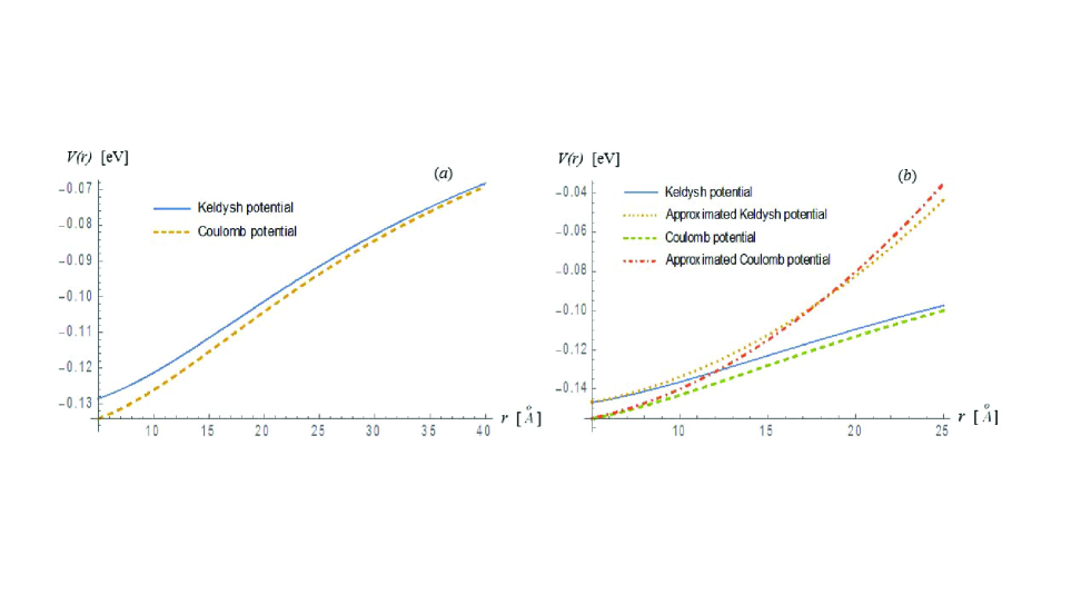
Figure 2: (Color online) (a) The Keldysh and Coulomb potentials for electron-hole attraction in a black phosphorene double layer. (b) Comparison of the Keldysh and Coulomb electron-hole attractions in a black phosphorene double layer approximated by the harmonic oscillator potential. The calculations were performed for the number $N_{L}=7$ of $h$-BN monolayers, placed between two phosphorene monolayers, the set of masses from Ref. Peng2014 and polarizability from Ref. Rodin .

For the number $N_{L}=7$ of $h$-BN monolayers, placed between two phosphorene monolayers, the binding energies of dipolar excitons, calculated for the sets of the masses from Refs. [Peng2014, ; Tran2014-2, ; Paez2014, ; Qiao2014, ] by using Eq. (15), are given by $28.2\ \mathrm{meV}$, $29.6\ \mathrm{meV}$, $37.6\ \mathrm{meV}$, and $37.2\ \mathrm{meV}$. Let us mention that the maximal dipolar exciton binding energy was obtained for the set of the masses, taken from Ref. [Qiao2014, ]. The dipolar exciton binding energy increases when the reduced mass $\mu_{0}$ of the exciton reduced masses increases. The reduced mass $\mu_{0}$ for the sets of the masses from Refs. [Peng2014, ; Tran2014-2, ; Paez2014, ; Qiao2014, ] is presented in Table 2. One can conclude that while $D_{0}$ is not sensitive to the choice of the set of effective electrons and holes masses, the binding energy of indirect exciton depends on the exciton reduced mass $\mu_{0}$, which is defined by the effective electron and hole masses.

It is worthy of note that the energy spectrum of the center-of-mass of an electron-hole pair $\varepsilon_{0}(\mathbf{P})$ may be expressed as

$$\varepsilon_{0}(\mathbf{P})=\frac{P_{x}^{2}}{2M_{x}}+\frac{P_{y}^{2}}{2M_{y}}.$$ (18)

Substituting the polar coordinate for the momentum $P_{x}=P\cos\Theta$ and $P_{y}=P\sin\Theta$ into Eq. (18), we obtain

$$\varepsilon_{0}(\mathbf{P})=\varepsilon_{0}(P,\Theta)=\frac{P^{2}}{2M_{0}(\Theta)},$$ (19)

where $M_{0}(\Theta)$ is the effective angle-dependent exciton mass in a black phosphorene double layer, given by

$$M_{0}(\Theta)=\left[\frac{\cos^{2}\Theta}{M_{x}}+\frac{\sin^{2}\Theta}{M_{y}}\right]^{-1}.$$ (20)

III Collective excitations for dipolar excitons in a black phosphorene double layer

We now turn our attention to a dilute distribution of electrons and holes in a pair of parallel black phosphorene layers spatially separated by a dielectric, when $nr_{X}^{2}\ll 1$, where $n$ is the concentration for dipolar excitons. In this limit, the dipolar excitons are formed by electron-hole pairs with the electrons and holes spatially separated in two different phosphorene layers.

The distinction between excitons, which are not an elementary but a composite bosons Comberscot and bosons is caused by exchange effects Moskalenko_Snoke . At large interlayer separations $D$, the exchange effects in the exciton-exciton interactions in a phosphorene double layer can be neglected, since the exchange interactions in a spatially separated electron-hole system in a double layer are suppressed due to the low tunneling probability, caused by the shielding of the dipole-dipole interaction by the insulating barrier BK ; BLG . Therefore, we treat the dilute system of dipolar excitons in a phosphorene double layer as a weakly interacting Bose gas.

The model Hamiltonian $\hat{H}$ of the 2D interacting dipolar excitons is given by

$$\hat{H}=\sum_{\mathbf{P}}\varepsilon_{0}(P,\Theta)a_{\mathbf{P}}^{\dagger}a_{\mathbf{P}}+\frac{g}{S}\sum_{\mathbf{P}_{1}\mathbf{P}_{2}\mathbf{P}_{3}}a_{\mathbf{P}_{1}}^{\dagger}a_{\mathbf{P}_{2}}^{\dagger}a_{\mathbf{P}_{3}}a_{\mathbf{P}_{1}+\mathbf{P}_{2}-\mathbf{P}_{3}},$$ (21)

where $a_{\mathbf{P}}^{\dagger}$ and $a_{\mathbf{P}}$ are Bose creation and annihilation operators for dipolar excitons with momentum $\mathbf{P}$, $S$ is a normalization area for the system, $\varepsilon_{0}(P,\Theta)$ is the angular-dependent energy spectrum of non-interacting dipolar excitons, given by Eq.  (19), and $g$ is a coupling constant for the interaction between two dipolar excitons.

We expect that at $T=0$ K almost all dipolar excitons condense into a BEC. One can treat this weakly interacting gas of dipolar excitons within the Bogoliubov approximation Abrikosov ; Lifshitz . The Bogoliubov approximation for a weakly interacting Bose gas allows us to diagonalize the many-particle Hamiltonian, replacing the product of four operators in the interaction term by the product of two operators. This is justified under the assumption that most of the particles belong to the BEC, and only the interactions between the condensate and non-condensate particles are taken into account, while the interactions between non-condensate particles are neglected. The condensate operators are replaced by numbers Abrikosov , and the resulting Hamiltonian is quadratic with respect to the creation and annihilation operators. Employing the Bogoliubov approximation Lifshitz , we obtain the chemical potential $\mu$ of the entire exciton system by minimizing $\hat{H}_{0}-\mu\hat{N}$ with respect to the 2D concentration $n$, where $\hat{N}$ denotes the number operator. The later one is

$$\hat{N}=\sum_{\mathbf{k}}a_{\mathbf{P}}^{\dagger}a_{\mathbf{P}},$$ (22)

while $H_{0}$ is the Hamiltonian describing the particles in the condensate with zero momentum $\mathbf{P}=0$. The minimization of $\hat{H}_{0}-\mu\hat{N}$ with respect to the number of excitons $N=Sn$ results in the standard expression Abrikosov ; Lifshitz

$$\mu=gn.$$ (23)

Following the procedure presented in Ref. [BKKL, ], the interaction parameters for the exciton-exciton interaction in very dilute systems could be obtained assuming the exciton-exciton dipole-dipole repulsion exists only at distances between excitons greater than distance from the exciton to the classical turning point. The distance between two excitons cannot be less than this distance, which is determined by the conditions reflecting the fact that the energy of two excitons cannot exceed the doubled chemical potential $\mu$ of the system, i.e.,

$$U(R_{0})=2\mu.$$ (24)

In Eq. (24) $U(R_{0})$ is the potential of interaction between two dipolar excitons at the distance $R_{0}$, where $R_{0}$ corresponds to the distance between two dipolar excitons at their classical turning point.

For our model we investigate the formation of dipolar excitons in a phosphorene double layer with the use of the Keldysh and Coulomb interactions. Therefore, it is reasonable to adopt the general approach for treating collective excitations of dipolar excitons. If the distance between two dipolar excitons is $R$ and the electron and hole of one dipolar exciton interact with the electron and hole of the other dipolar exciton, it is straightforward to show that the exciton-exciton interaction $U(R)$ has the form:

$$U(R)=2V(R)-2V\left(R\sqrt{1+\frac{D^{2}}{R^{2}}}\right),$$ (25)

where $V(R)$ represents the interaction potential between two electrons or two holes in the same phosphorene monolayer. We can assume the potential $V(R)$ to be given by either Keldysh potential (6) or by Coulomb potential.

In a very dilute system of dipolar excitons and, therefore, $D\ll R$, one may expand the second term in Eq. (25) in terms of $(D/R)^{2},$ and by retaining only the first order terms with respect to $(D/R)^{2}$, finally obtains

$$U(R)=\left\{\begin{array}[]{c}\frac{\pi ke^{2}D^{2}}{2\varepsilon_{d}\rho_{0}^{2}R}\left[Y_{-1}\left(\frac{R}{\rho_{0}}\right)-H_{-1}(y)\left(\frac{R}{\rho_{0}}\right)\right],\text{ for the Keldysh potential, }\\ \frac{ke^{2}D^{2}}{\epsilon_{d}R^{3}},\text{ \ \ \ \ \ \ \ \ \ \ \ \ \ \ \ \ \ \ \ \ \ \ \ \ \ \ \ \ \ \ \ \ \ \ \ \ \ \ for the Coulomb potential.}\end{array}\right.$$ (28)

Following the procedure presented in Ref. [BKKL, ], one can obtain the coupling constant for the exciton-exciton interaction:

$$g=2\pi\int_{R_{0}}^{\infty}RdR\ U(R).$$ (29)

Substituting Eq.  (28) into Eq.  (29), one obtains the exciton-exciton coupling constant $g$ as following

$$g=\left\{\begin{array}[]{c}\frac{2\pi^{2}ke^{2}D^{2}}{2\epsilon_{d}\rho_{0}}\left[H_{0}\left(\frac{R_{0}}{\rho_{0}}\right)-Y_{0}\left(\frac{R_{0}}{\rho_{0}}\right)\right],\text{ for the Keldysh potential,}\\ \frac{2\pi ke^{2}D^{2}}{\epsilon_{d}R_{0}},\text{ \ \ \ \ \ \ \ \ \ \ \ \ \ \ \ \ \ \ \ \ \ \ \ \ \ \ \ \ \ \ \ \ for the Coulomb potential.}\end{array}\right.$$ (32)

Combining Eqs. (24), (28) and (32), for the Keldysh potential we obtain the following equation for $R_{0}$:

$$4\pi n\rho_{0}^{2}y\left[H_{0}(y)-Y_{0}(y)\right]=-\left[H_{-1}(y)-Y_{-1}(y)\right],$$ (33)

where $y=R_{0}/\rho_{0}$.

Combining Eqs. (24), (28) and (32), we obtain the following expression for $R_{0}$ in the case of Coulomb potential

$$R_{0}=\frac{1}{2\sqrt{\pi n}}.$$ (34)

From Eqs. (34), (32) and (23), one obtains the exciton-exciton coupling constant $g$ for the Coulomb potential

$$g=\frac{4\pi ke^{2}D^{2}\sqrt{\pi n}}{\epsilon_{d}}.$$ (35)

The coupling constant $g$ and the distance $R_{0}$ between two dipolar excitons at the classical turning point for the Keldysh and Coulomb potentials for a phosphorene double layer as functions of the exciton concentration are represented in Fig. 3. According to Fig. 3, $R_{0}$ decreases with the increase of the exciton concentration $n$. While for the Coulomb potential $R_{0}$ is slightly larger than for the Keldysh potential, the difference is very small. As shown in Fig. 3, the coupling constant $g$ is larger for the Coulomb potential than for the Keldysh potential, because the interaction between the charge carriers, interacting via the Kledysh potential, is suppressed by the screening effects. The difference between $g$ for the Keldysh and Coulomb potentials increases as the exciton concentration $n$ increases.

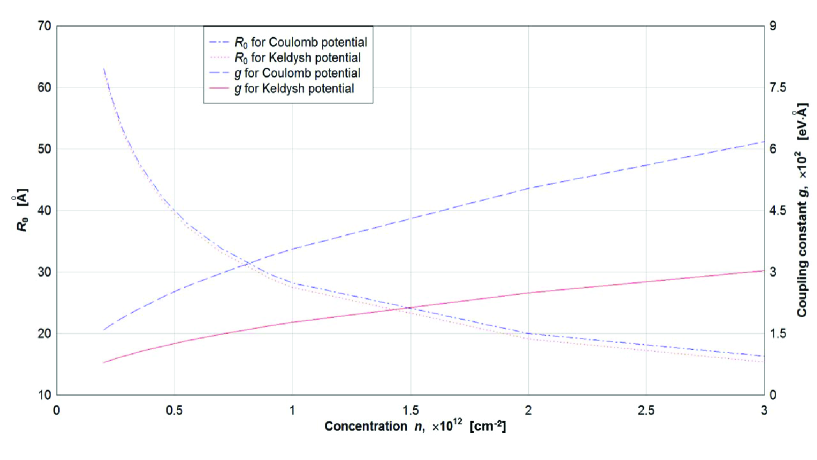
Figure 3: (Color online) The coupling constant $g$ and the distance $R_{0}$ between two dipolar excitons at the classical turning point for the Keldysh and Coulomb potentials for a phosphorene double layer as functions of the exciton concentration. The number of $h$-BN monolayers between the phosphorene monolayers is $N_{L}=7$.

The many-particle Hamiltonian of dipolar excitons in a black phosphorene double layer given by Eq.  (21) is standard for a weakly interacting Bose gas with the only difference being that the single-particle energy spectrum of non-interacting excitons is angular-dependent due to the orientation variation of the exciton effective mass. Whereas the first term in Eq.  (21) which is responsible for the single-particle kinetic energy is angular dependent, the second interaction term in Eq.  (21) does not depend on an angle because the dipole-dipole repulsion between excitons does not depend on an angle. Therefore, for a weakly interacting gas of dipolar excitons in a black phosphorene double layer, in the framework of the Bogoliubov approximation, we could apply exactly the same procedure which has been adapted for a standard weakly interacting Bose gas Abrikosov ; Lifshitz , but taking into account the angular dependence of a single-particle energy spectrum of dipolar excitons. Therefore, the Hamiltonian $\hat{H}_{col}$ of the collective excitations in the Bogoliubov approximation for the weakly interacting gas of dipolar excitons in black phosphorene is given by

$$\hat{H}_{col}=\sum_{P\neq 0,\Theta}\varepsilon(P,\Theta)\alpha_{\mathbf{P}}^{\dagger}\alpha_{\mathbf{P}},$$ (36)

where $\alpha_{j\mathbf{P}}^{\dagger}$ and $\alpha_{j\mathbf{P}}$ are the creation and annihilation Bose operators for the quasiparticles with the energy dispersion corresponding to the angular dependent spectrum of the collective excitations $\varepsilon(P,\Theta)$, described by

$$\varepsilon(P,\Theta)=\left[\left(\varepsilon_{0}(P,\Theta)+gn\right)^{2}-\left(gn\right)^{2}\right]^{1/2}.$$ (37)

In the limit of small momenta $P$, when $\varepsilon_{0}(P,\Theta)\ll gn$, we expand the spectrum of collective excitations $\varepsilon(P,\Theta)$ up to first order with respect to the momentum $P$ and obtain the sound mode of the collective excitations $\varepsilon(P,\Theta)=c_{S}(\Theta)P$, where $c_{S}(\Theta)$ is the angular dependent sound velocity, given by

$$c_{S}(\Theta)=\sqrt{\frac{gn}{M_{0}(\Theta)}}.$$ (38)

The asymmetry of the electron and hole dispersion in black phosphorene is reflected in the angular dependence of the sound velocity through the angular dependence of the effective exciton mass. The angular dependence of the sound velocity for the Keldysh and Coulomb potentials is presented in Fig. 4, where it is demonstrated that the exciton sound velocity is maximal at $\Theta=0$ and $\Theta=\pi$ and minimal at $\Theta=\pi/2$. As it follows from comparison of Fig. 4a with Fig. 4b, at the same parameters, the sound velocity $c_{S}(\Theta)$ is greater in the case of Coulomb potential for the interaction between the charge carriers than for the Keldysh potential, because the Keldysh potential implies the screening effects, which make the interaction between the carriers weaker. According to Fig. 4, the sound velocity depends on the effective electron and hole masses. However, the sound velocities are coincided at all angles $\Theta$ for two sets of masses from Refs. [Paez2014, ] and [Qiao2014, ], correspondingly. Since at low momenta the sound-like energy spectrum of collective excitations in the dipolar exciton system in a phosphorene double layer satisfies to the Landau criterion for superfluidity, the dipolar exciton superfluidity in a black phosphorene double layer is possible. Let us mention that the exciton concentration, used for the calculations, represented in Fig. 4 and below, corresponds by the order of magnitude to the experimental values Warren ; Surrente .

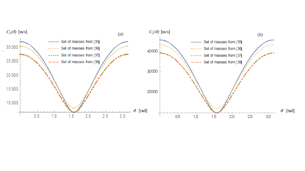
Figure 4: (Color online) The angular dependence of the sound velocity. (a) The interaction between the carriers is described by the Keldysh potential. (b) The interaction between the carriers is described by the Coulomb potential. The calculations were performed for the exciton concentration $n=2\times 10^{16}\ \mathrm{m^{-2}}$ and the number $N_{L}=7$ of $h$-BN monolayers, placed between two phosphorene monolayers.

IV Superfluidity of dipolar excitons in a black phosphorene double Layer

Since, at small momenta, the energy spectrum of the quasiparticles for a weakly interacting gas of dipolar excitons is sound-like, this means that the system satisfies to the Landau criterion for superfluidity Abrikosov ; Lifshitz . The critical exciton velocity for superfluidity is angular-dependent, and it is given by $v_{c}(\Theta)=c_{S}(\Theta)$, because the quasiparticles are created at velocities above the angle dependent velocity of sound. According to Fig. 4, the critical exciton velocity for superfluidity has maximum at $\Theta=0$ and $\Theta=\pi$ and has minimum at $\Theta=\pi/2$. Therefore, as shown in Fig. 4a, if the excitons move with the velocities in the range of approximately between $8\times 10^{3}\ \mathrm{m/s}$ and $3.4\times 10^{4}\ \mathrm{m/s}$, the superfluity is present for the angles at the edges of the angle range between $\Theta=0$ and $\Theta=\pi$, while the superfluidity is absent at the center of this angle range.

The density of the superfluid component $\rho_{s}(T)$ is defined as $\rho_{s}(T)=\rho-\rho_{n}(T)$, where $\rho$ is the total 2D density of the system and $\rho_{n}(T)$ is the density of the normal component. We define the normal component density $\rho_{n}(T)$ in the usual way.Pitaevskii . Suppose that the excitonic system moves with a velocity $\mathbf{u}$, which means that the superfluid component moves with the velocity $\mathbf{u}$. At nonzero temperatures $T$ dissipating quasiparticles will appear in this system. Since their density is small at low temperatures, one may assume that the gas of quasiparticles is an ideal Bose gas. To calculate the superfluid component density, we define the total mass current $\mathbf{J}$ for a Bose-gas of quasiparticles in the frame of reference where the superfluid component is at rest, by

$$\mathbf{J}=\int\frac{sd^{2}P}{(2\pi\hbar)^{2}}\mathbf{P}f\left[\varepsilon(P,\Theta)-\mathbf{P}\mathbf{u}\right].$$ (39)

In Eq. (39) $f\left[\varepsilon(P,\Theta)\right]=\left(\exp\left[\varepsilon(P,\Theta)/(k_{B}T)\right]-1\right)^{-1}$ is the Bose-Einstein distribution function for quasiparticles with the angule dependent dispersion $\varepsilon(P,\Theta)$, $s=4$ is the spin degeneracy factor, and $k_{B}$ is the Boltzmann constant. Expanding the integrand of Eq. (39) in terms of $\mathbf{P}\mathbf{u}/(k_{B}T)$ and restricting ourselves by the first order term, we obtain

$$\mathbf{J}=-\frac{s}{k_{B}T}\int\frac{d^{2}P}{(2\pi\hbar)^{2}}\mathbf{P}\left(\mathbf{Pu}\right)\frac{\partial f\left[\varepsilon(P,\Theta)\right]}{\partial\varepsilon(P,\Theta)}.$$ (40)

The normal density $\rho_{n}$ in the anisotropic system has tensor form Saslow . We define the tensor elements for the normal component density $\rho_{n}^{(ij)}(T)$ by

$$J_{i}=\rho_{n}^{(ij)}(T)u_{j},$$ (41)

where $i$ and $j$ denote either the $x$ or $y$ component of the vectors. Assuming that the vector ${\bf u}\uparrow\uparrow OX$ ($\uparrow\uparrow$ denotes that ${\bf u}$ is parallel to the $OX$ axis and has the same direction as the $OX$ axis), we have ${\bf u}=u_{x}{\bf i}$ and ${\bf P}=P_{x}{\bf i}+P_{y}{\bf j}$. Therefore, we obtain

$${\bf P}\cdot{\bf u} = P_{x}u_{x},$$

$${\bf P}\left({\bf P}\cdot{\bf u}\right) = P_{x}^{2}u_{x}{\bf i}+P_{x}P_{y}u_{x}{\bf j},$$ (42)

where ${\bf i}$ and ${\bf j}$ are unit vectors in the $x$ and $y$ directions, respectively. Upon substituting Eq. (42) into Eq. (40), one obtains

$$J_{x}=-\frac{s}{k_{B}T}\int_{0}^{\infty}dP\frac{P^{3}}{(2\pi\hbar)^{2}}\int_{0}^{2\pi}d\Theta\frac{\partial f\left[\varepsilon(P,\Theta)\right]}{\partial\varepsilon(P,\Theta)}\cos^{2}\Theta u_{x}.$$ (43)

Using the definition of the density for the normal component from Eq. (41), we obtain

$$\rho_{n}^{(xx)}(T)=\frac{s}{k_{B}T}\int_{0}^{\infty}dP\frac{P^{3}}{(2\pi\hbar)^{2}}\int_{0}^{2\pi}d\Theta\frac{\exp\left[\varepsilon(P,\Theta)/(k_{B}T)\right]}{\left(\exp\left[\varepsilon(P,\Theta)/(k_{B}T)\right]-1\right)^{2}}\cos^{2}\Theta.$$ (44)

Substitution of Eq. (42) into Eq. (40) gives

$$J_{y} = -\frac{s}{k_{B}T}\int\frac{d^{2}P}{(2\pi\hbar)^{2}}P_{x}P_{y}\frac{\partial f\left[\varepsilon(P,\Theta)\right]}{\partial\varepsilon(P,\Theta)}u_{x}$$ (45)

$$= \frac{s}{k_{B}T}\int_{0}^{\infty}dP\frac{P^{3}}{(2\pi\hbar)^{2}}\int_{0}^{2\pi}d\Theta\frac{\exp\left[\varepsilon(P,\Theta)/(k_{B}T)\right]}{\left(\exp\left[\varepsilon(P,\Theta)/(k_{B}T)\right]-1\right)^{2}}\cos\Theta\sin\Theta u_{x}=0.$$

The integral in Eq. (45) equals to zero, since the integral over the angle $\Theta$ over the period of the function results in zero. Therefore, one obtains $\rho_{n}^{(xy)}=0$.

Now assuming the vector ${\bf u}\uparrow\uparrow OY$, we obtain analogously the following relations:

$$\rho_{n}^{(yy)}(T) = \frac{s}{k_{B}T}\int_{0}^{\infty}dP\frac{P^{3}}{(2\pi\hbar)^{2}}\int_{0}^{2\pi}d\Theta\frac{\exp\left[\varepsilon(P,\Theta)/(k_{B}T)\right]}{\left(\exp\left[\varepsilon(P,\Theta)/(k_{B}T)\right]-1\right)^{2}}\sin^{2}\Theta,$$

$$\rho_{n}^{(yx)}(T) = 0\ .$$ (46)

By defining the tensor of the concentration of the normal component as the linear response of the flow of quasiparticles on the external velocity as $n_{n}^{(ij)}=\rho_{n}^{(ij)}/M_{i}$, one obtains:

$$n_{n}^{(xx)}(T) = \frac{s}{k_{B}M_{x}T}\int_{0}^{\infty}dP\frac{P^{3}}{(2\pi\hbar)^{2}}\int_{0}^{2\pi}d\Theta\frac{\exp\left[\varepsilon(P,\Theta)/(k_{B}T)\right]}{\left(\exp\left[\varepsilon(P,\Theta)/(k_{B}T)\right]-1\right)^{2}}\cos^{2}\Theta,$$

$$n_{n}^{(xy)}(T) = 0\$$

$$n_{n}^{(yy)}(T) = \frac{s}{k_{B}M_{y}T}\int_{0}^{\infty}dP\frac{P^{3}}{(2\pi\hbar)^{2}}\int_{0}^{2\pi}d\Theta\frac{\exp\left[\varepsilon(P,\Theta)/(k_{B}T)\right]}{\left(\exp\left[\varepsilon(P,\Theta)/(k_{B}T)\right]-1\right)^{2}}\sin^{2}\Theta,$$

$$n_{n}^{(yx)}(T) = 0.$$ (47)

The linear response of the flow of quasiparticles $\mathbf{J}_{qp}$ with respect to the external velocity at any angle measured from the $OX$ direction is given in terms of the angle dependent concentration for the normal component $\tilde{n}_{n}(\Theta,T)$ as

$$\left|\mathbf{J}_{qp}\right| = \left|n_{n}^{(xx)}(T)u_{x}{\bf i}+n_{n}^{(yy)}(T)u_{y}{\bf j}\right|$$ (48)

$$= \sqrt{\left[n_{n}^{(xx)}(T)\right]^{2}u^{2}\cos^{2}\Theta+\left[n_{n}^{(yy)}(T)\right]^{2}u^{2}\sin^{2}\Theta}=\tilde{n}(\Theta,T)u,$$

where the concentration of the normal component $\tilde{n}_{n}(\Theta,T)$ is

$$\tilde{n}_{n}(\Theta,T)=\sqrt{\left[n_{n}^{(xx)}(T)\right]^{2}\cos^{2}\Theta+\left[n_{n}^{(yy)}(T)\right]^{2}\sin^{2}\Theta}.$$ (49)

From Eq. (49) it follows that $n_{n}^{(xx)}=\tilde{n}_{n}(\Theta=0)$ and $n_{n}^{(yy)}=\tilde{n}_{n}(\Theta=\frac{\pi}{2})$.

Eq. (49) can be rewritten in the following form:

$$\tilde{n}_{n}(\Theta,T)=\sqrt{\frac{\left[n_{n}^{(xx)}(T)\right]^{2}+\left[n_{n}^{(yy)}(T)\right]^{2}}{2}+\frac{\left(\left[n_{n}^{(xx)}(T)\right]^{2}-\left[n_{n}^{(yy)}(T)\right]^{2}\right)\cos\left(2\Theta\right)}{2}}.$$ (50)

We define the angle dependent concentration of the superfluid component $\tilde{n}_{s}(\Theta,T)$ by

$$\tilde{n}_{s}(\Theta,T)=n-\tilde{n}_{n}(\Theta,T),$$ (51)

where $n$ is the total concentration of the dipolar excitons. The mean field critical temperature $T_{c}(\Theta)$ of the phase transition related to the occurrence of superfluidity in the direction with the angle $\Theta$ relative to the $x$ direction is determined by the condition

$$\tilde{n}_{n}(\Theta,T_{c}(\Theta))=n.$$ (52)

IV.1 Superfluidity for the sound-like spectrum of collective excitations

For small momenta, substituting the sound spectrum of collective excitations $\varepsilon(P,\Theta)=c_{S}(\Theta)P$ with the angular-dependent sound velocity $c_{S}(\Theta)$, given by Eq. (38), into Eq. (47), we obtain

$$n_{n}^{(xx)}(T) = \frac{2s(k_{B}T)^{3}\zeta(3)}{(\pi\hbar)^{2}M_{x}}\int_{0}^{2\pi}\frac{\cos^{2}\Theta}{c_{S}^{4}(\Theta)}d\Theta=\frac{2s(k_{B}T)^{3}\zeta(3)}{(\pi\hbar gn)^{2}M_{x}}\int_{0}^{2\pi}\frac{\cos^{2}\Theta}{\left(\frac{\cos^{2}\Theta}{M_{x}}+\frac{\sin^{2}\Theta}{M_{y}}\right)^{2}}d\Theta,$$

$$n_{n}^{(xy)}(T) = 0,$$

$$n_{n}^{(yy)}(T) = \frac{2s(k_{B}T)^{3}\zeta(3)}{(\pi\hbar)^{2}M_{y}}\int_{0}^{2\pi}\frac{\sin^{2}\Theta}{c_{S}^{4}(\Theta)}d\Theta=\frac{2s(k_{B}T)^{3}\zeta(3)}{(\pi\hbar gn)^{2}M_{y}}\int_{0}^{2\pi}\frac{\sin^{2}\Theta}{\left(\frac{\cos^{2}\Theta}{M_{x}}+\frac{\sin^{2}\Theta}{M_{y}}\right)^{2}}d\Theta,$$

$$n_{n}^{(yx)}(T) = 0,$$ (53)

where $\zeta(z)$ is the Riemann zeta function ($\zeta(3)\simeq 1.202$).

The integrals in Eq. (53) can be evaluated analytically. Substituting the following expressions

$$\int_{0}^{2\pi}\frac{\cos^{2}\Theta}{\left(\frac{\cos^{2}\Theta}{M_{x}}+\frac{\sin^{2}\Theta}{M_{y}}\right)^{2}}d\Theta=\pi M_{x}\sqrt{M_{x}M_{y}},\hskip 56.9055pt\int_{0}^{2\pi}\frac{\sin^{2}\Theta}{\left(\frac{\cos^{2}\Theta}{M_{x}}+\frac{\sin^{2}\Theta}{M_{y}}\right)^{2}}d\Theta=\pi M_{y}\sqrt{M_{x}M_{y}},$$ (54)

into Eq. (53), one obtains

$$n_{n}^{(xx)}(T)=n_{n}^{(yy)}(T)=\frac{2\zeta(3)s(k_{B}T)^{3}\sqrt{M_{x}M_{y}}}{\pi(\hbar gn)^{2}},\hskip 56.9055ptn_{n}^{(xy)}(T)=n_{n}^{(yx)}(T)=0.$$ (55)

Let us mention that Eq. (54) is valid if $\frac{M_{x}}{2\left(M_{y}-M_{x}\right)}>0$, which is true for a phosphorene double layer. Note that for the anisotropic superfluid, formed by paired fermions, the relation $n_{n}^{(xx)}(T)=n_{n}^{(yy)}(T)$ is also valid Saslow .

Under the assumption of the sound spectrum of collective excitations using Eq. (55), implying $n_{n}^{(xx)}(T)=n_{n}^{(yy)}(T)$, one obtains from Eq. (49) the concentration of the normal component $\tilde{n}_{n}(T)$ as

$$\tilde{n}_{n}(T)=n_{n}^{(xx)}(T)=n_{n}^{(yy)}(T)=\frac{2\zeta(3)s(k_{B}T)^{3}\sqrt{M_{x}M_{y}}}{\pi(\hbar gn)^{2}}.$$ (56)

Therefore, in case of the sound-like spectrum of collective excitations, the concentration of the superfluid component $\tilde{n}_{s}(T)$ is given by

$$\tilde{n}_{s}(T)=n-\frac{2\zeta(3)s(k_{B}T)^{3}\sqrt{M_{x}M_{y}}}{\pi(\hbar gn)^{2}}.$$ (57)

It follows from Eqs. (56) and (57) that for the sound-like spectrum of collective excitations, the concentrations of the normal and superfluid components do not depend on an angle.

For the sound-like spectrum of collective excitations, the mean field critical temperature $T_{c}$ can be obtained by substitution Eq. (56) into the condition $\tilde{n}_{n}(T_{c})=n$ as following

$$T_{c}=\left(\frac{\pi(\hbar g)^{2}}{2\zeta(3)s\sqrt{M_{x}M_{y}}}\right)^{1/3}\frac{n}{k_{B}}.$$ (58)

It follows from Eq. (58) that under the assumption about the sound-like spectrum of collective excitations, the mean field critical temperature $T_{c}$ does not depend on an angle. The mean field critical temperature of the superfluidity $T_{c}$ for the Keldysh and Coulomb potentials for the sound-like spectrum of collective excitations obtained by using Eq. (58) as a function of the interlayer separation $D$, is presented in Fig. 5. The calculations are performed for the sets of effective electron and hole masses from Refs. Peng2014, ; Tran2014-2, ; Paez2014, ; Qiao2014, . Comparing Fig. 5a with Fig. 5b, one concludes that at the same parameters, the critical temperature for the superfluidity $T_{c}(\Theta)$ is much larger for the Coulomb potential than for the Keldysh potential, because the sound velocity for the Coulomb potential is larger than for the Kelsysh potential due to the screening effects, implied by the Keldysh potential. However, for both potentials the mean field critical temperature for superfluidity shows the similar depends on the electron and hole effective masses.

Table 2: The critical temperatures under the assumption about the sound-like spectrum of collective excitations for different sets of masses from Refs. Peng2014 , Tran2014-2 , Paez2014 , and Qiao2014 . The phosphorene layers are separated by 7 layers of h-BN. $\mu_{0}$ and $M_{x}M_{y}$ are expressed in units of free electron mass $m_{0}$ and $m_{0}^{2},$ respectively.

Mass from Ref:	Peng2014	Tran2014-2	Paez2014	Qiao2014
$\mu_{0},$ $\times$10${}^{-2}m_{0}$	3.99	4.11	4.84	4.79
Coulomb potential $T_{c},$ K	182	192	174	172
Keldysh potential $T_{c},$ K	115	121	109	107
$M_{x}M_{y},$ $\times m_{0}^{2}$	1.67	1.23	2.24	2.39

As it is demonstrated in Table 2, the critical temperature for the superfluidity $T_{c}$ decreases when $M_{x}M_{y}$ increases. Therefore, $T_{c}$ is sensitive to the electron and hole effective masses.

Assuming the sound-like spectrum of collective excitations, the mean field critical temperature of the superfluidity $T_{c}$ obtained by using Eq. (58) as a function of the exciton concentration $n$ and the interlayer separation $D$, is presented in Fig. 6. While the calculations, presented in Fig. 6, were performed for the Coulomb potential, one can obtain the similar behavior for the mean field critical temperature of the superfluidity by employing the Keldysh potential. According to Figs. 5 and 6, the mean field critical temperature of the superfluidity $T_{c}$ is an increasing function of the exciton concentration $n$ and the interlayer separation $D$.

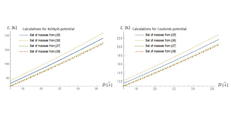
Figure 5: (Color online) The mean field critical temperature for superfluidity $T_{c}$ for a phosphorene double layer as a function of the interlayer separation $D$, assuming the sound-like spectrum of collective excitations. (a) The interaction between the carriers is described by the Keldysh potential. (b) The interaction between the carriers is described by the Coulomb potential. The exciton concentration is $n=2\times 10^{12}\ \mathrm{cm^{-2}}$.

Figure 6: (Color online) The critical temperature for superfluidity $T_{c}$ for a phosphorene double layer as a function of the exciton concentration $n$ and the interlayer separation $D$, assuming the sound-like spectrum of collective excitations. The calculations are performed for the Coulomb potential. The set of masses is taken from Ref. [Paez2014, ].

IV.2 Superfluidity when the spectrum of collective excitations is given by Eq. (37)

Beyond the assumption of the sound-like spectrum, substituting Eq. (37) for the spectrum of collective excitations into Eq. (47), and using Eq. (50), we obtain the mean field critical temperature of the superfluidity $T_{c}(\Theta)$, by solving numerically Eq. (52). Since in this case $n_{n}^{(xx)}(T)\neq n_{n}^{(yy)}(T)$, the mean field critical temperature of the superfluidity $T_{c}(\Theta)$ is angular dependent. The angular dependence of critical temperature $T_{c}(\Theta)$ for the Keldysh and Coulomb potentials for different exciton concentrations, calculated by solution of transcendental equation (52), is presented in Fig. 7. According to Fig. 7, the mean field critical temperature of the superfluidity $T_{c}(\Theta)$, is an increasing function of the exciton concentration $n$. According to Fig. 7, the critical critical temperature of the superfluidity is maximal at $\Theta=0$ and $\Theta=\pi$ and minimal at $\Theta=\pi/2$.

As it follows from comparison of Fig. 7a with Fig. 7b, at the same parameters, the mean field critical temperature for the superfluidity $T_{c}(\Theta)$ is greater when one considers the Coulomb potential for the interaction between the charge carriers than for the Keldysh potential, because the sound velocity for the Coulomb potential is greater than for the Keldysh potential due to the screening effects, taken into account by the Keldysh potential.

It is interesting to mention that the ratio of the maximal critical temperature $T_{c}^{(\mathrm{max})}=T_{c}(0)$ to the minimal critical temperature $T_{c}^{\mathrm{(min)}}=T_{c}(\pi/2)$, $T_{c}^{(\mathrm{max})}/T_{c}^{\mathrm{(min)}}$, in case of both the Keldysh and Coulomb interactions between the charge carriers decreases from $3.55$ to $2.69$ for the Keldysh potential, and from $3.29$ to $2.64$ for the Coulomb potential, when the density of exciton increases from $n=2\times 10^{11}\ \mathrm{cm^{-2}}$ to $n=3\times 10^{12}\ \mathrm{cm^{-2}}$. One concludes that the angular dependence of the mean field critical temperature $T_{c}$ decreases, when the exciton concentration increases.

At the fixed exciton concentration $n$, at the temperatures below $T_{c}^{\mathrm{(min)}}$, exciton superfluidity exists at any direction of exciton motion with any angle $\Theta$ relative to the armchair direction, while at the temperatures above $T_{c}^{\mathrm{(max)}}$, exciton superfluidity is absent at any direction of exciton motion with any angle $\Theta$. At the fixed exciton concentration $n$, at the temperatures in the range $T_{c}^{\mathrm{(min)}}<T<T_{c}^{\mathrm{(max)}}$, exciton superfluidity exists only for the directions of exciton motion with the angles in the ranges $0<\Theta<\Theta_{c1}(T)$ and $\Theta_{c2}(T)<\Theta<\pi$, while the superfluidity is absent for the directions of exciton motion with the angles in the range $\Theta_{c1}(T)<\Theta<\Theta_{c2}(T)$. The critical angles of superfluidity $\Theta_{c1}(T)$ and $\Theta_{c2}(T)$ correspond in Fig. 7 to the left and right crossing points of the horizontal line at the temperature $T$ with the curve at the fixed exciton concentration $n$, respectively.

Let us mention that the critical temperature for the superfluidity for a BCS-like fermionic superfluid with the anisotropic order parameter does not depend on the direction of motion of Cooper pairs because in this case $n_{n}^{(xx)}(T)=n_{n}^{(yy)}(T)$ Saslow .

Let us mention that we chose to use the set of masses from Ref. [Paez2014, ], because this set results in higher exciton binding energy. We used the number of $h$-BN monolayers between the phosphorene monolayers $N_{L}=7$ for Figs. 4 and 7, because higher $N_{L}$ corresponds to higher interlayer separation $D$, which results in higher critical exciton velocity of superfluidity equal to the sound velocity $c_{S}(\Theta)$ and higher mean field critical temperature of the superfluidity $T_{c}(\Theta)$.

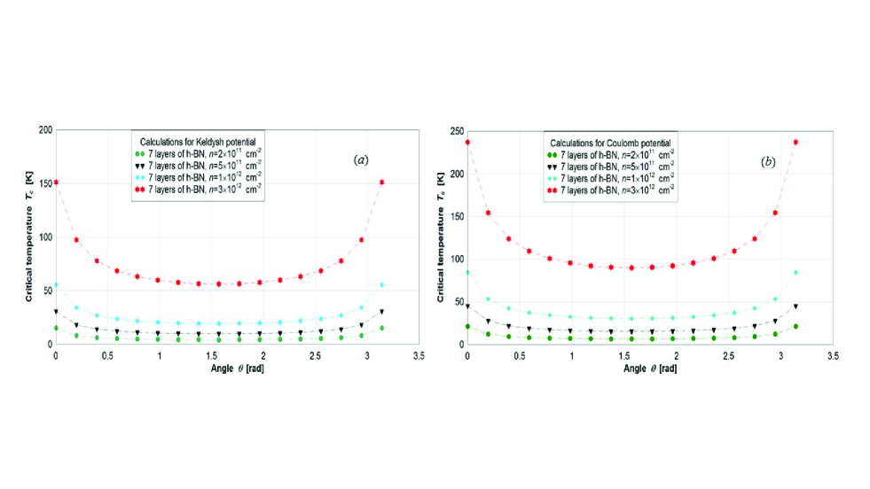
Figure 7: (Color online) The angular dependence of the critical temperature for superfluidity $T_{c}(\Theta)$ for a phosphorene double layer for different exciton concentrations. (a) The interaction between the carriers is described by the Keldysh potential. (b) The interaction between the carriers is described by the Coulomb potential. The number of $h$-BN monolayers between the phosphorene monolayers is $N_{L}=7$. The set of masses is taken from Ref. [Paez2014, ].

According to Eq. (50), the angular dependent concentration of the normal component $\tilde{n}_{n}(\Theta,T)$ for $0\leq\Theta\leq\pi/2$ increases with $\Theta$ if $n_{n}^{(yy)}(T)>n_{n}^{(xx)}(T)$ and decreases with $\Theta$ if $n_{n}^{(yy)}(T)<n_{n}^{(xx)}(T)$. Therefore, at $n_{n}^{(yy)}(T)>n_{n}^{(xx)}(T)$ the superfluidity can exist only if $\Theta<\Theta_{c}(T)$, while at $n_{n}^{(yy)}(T)<n_{n}^{(xx)}(T)$ the superfluidity can exist only if $\Theta>\Theta_{c}(T)$, where $\Theta_{c}(T)$ is the critical angle of the occurrence of superfluidity.

For a chosen temperature, the critical angle $\Theta_{c}(T)$, which corresponds to the occurrence of superfluidity, is given by the condition

$$\tilde{n}_{n}(\Theta_{c}(T),T)=n\ .$$ (59)

Substituting Eq. (50) into Eq, (59), one obtains a closed form analytic expression for $\Theta_{c}(T)$ as

$$\Theta_{c}(T)=\frac{1}{2}\arccos\left[\frac{2n^{2}-\left(\left[n_{n}^{(xx)}(T)\right]^{2}+\left[n_{n}^{(yy)}(T)\right]^{2}\right)}{\left[n_{n}^{(xx)}(T)\right]^{2}-\left[n_{n}^{(yy)}(T)\right]^{2}}\right]\ .$$ (60)

V Proposed experiment to observe the angular dependent superfluidity of dipolar excitons in a phosphorene Double Layer

The angular dependent superfluidity in a phosphorene double layer may be observed in electron-hole Coulomb drag experiments. The Coulomb attraction between electrons and holes can introduce a Coulomb drag that is a process in spatially separated conductors, which enables a current to flow in one of the layers to induce a voltage drop in the other one. In the case when the adjacent layer is part of a closed electrical circuit, an induced current flows. The experimental observation of exciton condensation and perfect Coulomb drag was claimed recently for spatially separated electrons and holes in GaAs/AlGaAs coupled quantum wells in the presence of high magnetic field perpendicular to the quantum wells Nandi . A steady transport current of electrons driven through one quantum well was accompanied by an equal current of holes in another. In Ref.  [Pogrebinskii, ], the authors discussed the drag of holes by electrons in a semiconductor-insulator-semiconductor structure. The prediction was that for two conducting layers separated by an insulator there will be a drag of carriers in one layer due to the direct Coulomb attraction with the carriers in the other layer. The Coulomb drag effect in the electron-hole double layer BCS system was also analyzed in Refs.  [VM, ; JBL, ]. If the external potential difference is applied to one of the layers, it will produce an electric current. The current in an adjacent layer will be initiated as a result of the correlations between electrons and holes at temperatures below the critical one. Consequently, the Coulomb drag effect was explored for semiconductor coupled quantum wells in a number of theoretical and experimental studies Gramila ; Sivan ; Gramila2 ; Jauho ; Zheng ; Sirenko ; Tso ; Flensberg ; Tanatar ; EMN . The Coulomb drag effect in two coaxial nanotubes was studied in Ref. [BGK, ]. The experimental and theoretical achievements in Coulomb drag effect have been reviewed in Ref. [Narrmp, ].

We propose to study experimentally the angular dependent superfluidity of dipolar excitons in a phosphorene double layer by applying a voltage difference for current flowing in one layer in a chosen direction at a chosen angle $\Theta$ relative to the armchair direction and measuring the drag current in the same direction in another layer. This drag current in another layer in the same direction as the current in the first layer will be initiated by the electron-hole Coulomb drag effect due to electron-hole attraction. The measurement of the drag current in an adjacent layer for a certain direction with the corresponding $\Theta$ will indicate the existence of superfluidity in this direction. Due to the angular dependence of the sound velocity, the critical exciton velocity for superfluidity depends on an angle. Therefore, for certain exciton velocities, there are the angle ranges, which correspond to the superfluid exciton flow, and other angle ranges, which correspond to the normal exciton flow. This can be applied as a working principal for switchers, controlling the exciton flows in different directions of exciton motion, caused by the Coulomb drag effect.

VI Conclusions

In summary, the influence of the anisotropy of the dispersion relation of dipolar excitons in a double layer of black phosphorene on the excitonic BEC and directional superfluidity has been investigated. The analytical expressions for the single dipolar exciton energy spectrum and wave functions have been derived. The angle dependent spectrum of collective excitations and sound velocity have been derived. It is predicted that a weakly interacting gas of dipolar excitons in a double layer of black phosphorus exhibits superfluidity at low temperatures due to the dipole-dipole repulsion between the dipolar excitons. It is concluded that the anisotropy of the energy band structure in a black phosphorene causes the critical velocity of the superfluidity to depend on the direction of motion of dipolar excitons. It is demonstrated that the dependence of the concentrations of the normal and superfluid components and the mean field critical temperatures for superfluidity on the direction of motion of dipolar excitons occurs beyond the sound-like approximation for the spectrum of collective excitations. Therefore, the directional superfluidity of dipolar excitons in a phosphorene double layer is possible. Moreover, the presented results, obtained for both Keldysh and Coilomb potentials, describing the interactions between the charge carriers, allow to study the influence of the screening effects on the dipolar exciton binding energy, exciton-exciton interaction, the spectrum of collective excitations, and the critical temperature of superfluidity for a weakly interacting Bose gas of dipolar excitons in a phosphorene double layer. It is important to mention that the binding energy of dipolar excitons, and mean field critical temperature for superfluidity are sensitive to the electron and hole effective masses. Besides, the possibilities of the experimental observation of the superfluidity for various directions of motion of excitons were briefly discussed.

Our analytical and numerical results provide motivation for future experimental and theoretical investigations on excitonic BEC and superfluidity for double layer phosohorene.

References

- (1) Yu. E. Lozovik and V. I. Yudson, Zh. Eksp. Teor. Fiz. 71, 738 (1976) [Sov. Phys. JETP 44, 389 (1976)]; Physica A 93, 493 (1978).
- (2) S. A. Moskalenko and D. W. Snoke, Bose-Einstein Condensation of Excitons and Biexcitons and Coherent Nonlinear Optics with Excitons (Cambridge University Press, New York, 2000; see also a recent review D. W. Snoke, ”Dipole excitons in coupled quantum wells: toward an equilibrium exciton condensate,” in Quantum Gases: Finite Temperature and Non-Equilibrium Dynamics (Vol. 1, Cold Atoms Series), N.P. Proukakis, S.A. Gardiner, M.J. Davis, and M.H. Szymanska, eds. (Imperial College Press, London, 2013).
- (3) M. Combescot, R. Combescot, and F. Dubin, Rep. Prog. Phys. 80, 066501 (2017).
- (4) M. M. Fogler, L. V. Butov, and K. S. Novoselov, Nature Commun. 5, 4555 (2014).
- (5) F. Wu, F. Qu, and A. H. MacDonald, Phys. Rev. B91, 075310 (2015).
- (6) O. L. Berman and R. Ya. Kezerashvili, Phys. Rev. B93, 245410 (2016).
- (7) A. H. Woomer, T. W. Farnsworth, J. Hu, R. A. Wells, C. L. Donley, and S. C. Warren, ACS Nano 9, 8869 (2015).
- (8) H. Liu, A. T. Neal, Z. Zhu, Z. Luo, X. Xu, and D. Tománek… ACS Nano, 8, 4033 (2014).
- (9) A. Jain and A. J. H. McGaughey, Scientific Reports 5, Article number: 8501 (2015).
- (10) H. Liu, A. T. Neal, Z. Zhu, Z. Luo, X. Xu, D. Tománek, and P. D. Ye, ACS Nano 8, 4033 (2014).
- (11) V. Tran, R. Soklaski, Y. Liang, and L. Yang, Phys. Rev. B 89, 235319 (2014).
- (12) J. Qiao, X. Kong, Z.-X. Hu, F. Yang, and W. Ji, Nature Communications 5, 4475 (2014).
- (13) P. Li and I. Appelbaum, Phys. Rev. B 90, 115439 (2014).
- (14) A. S. Rodin, A. Carvalho, and A. H. Castro Neto, Phys. Rev. B90, 075429 (2014).
- (15) A. Chaves, Tony Low, P. Avouris, D. Çakır, and F. M. Peeters, Phys. Rev. B 91, 155311 (2015).
- (16) F. Xia, H. Wang, and Y. Jia, Nature Communications 5, 4458 (2014).
- (17) Xiaomu Wang, Aaron M. Jones, Kyle L. Seyler, Vy Tran, Yichen Jia, Huan Zhao, Han Wang, Li Yang, Xiaodong Xu, and Fengnian Xia, Nature Nanotechnology 10, 517 (2015).
- (18) J .Y. Wu, Chen, G. Gumbs, and M. F. Lin, arxiv (2016).
- (19) Q. Wei and X. Peng, Applied Physics Letters, 104, 251915 (2014).
- (20) Ruixiang Fei and Li Yang, Nano Lett., , 14 (5), 2884 (2014).
- (21) Likai Li, Yijun Yu, Guo Jun Ye, Qingqin Ge, Xuedong Ou, Hua Wu, Donglai Feng, Xian Hui Chen, and Yuanbo Zhang, Nature Nanotechnology 9, 372 (2014).
- (22) L. V. Keldysh, Zh. Eksp. Teor. Fiz. Pis. Red. 29, 716 (1979) [JETP Lett. 29, 658 (1979)].
- (23) A. A. Abrikosov, L. P. Gorkov, and I. E. Dzyaloshinskii, Methods of Quantum Field Theory in Statistical Physics(Prentice-Hall, Englewood Cliffs, NJ, 1963).
- (24) W. M. Saslow, Phys. Rev. Lett. 31, 870 (1973).
- (25) P. Cudazzo, I. V. Tokatly, and A. Rubio, Phys. Rev. B84, 085406 (2011).
- (26) E. Prada, J. V. Alvarez, K.‘L. Narasimha-Acharya, F. J. Bailen, and J. J. Palacios, Phys. Rev. B91, 245421 (2015).
- (27) K.‘A. Velizhanin and A. Saxena, Phys. Rev. B92, 195305 (2015).
- (28) T. C. Berkelbach, M. S. Hybertsen, and D. R. Reichman, Phys. Rev. B88, 045318 (2013).
- (29) D.K. Zhang, D.W. Kidd, and K. Varga, Phys. Rev. B 93, 125423 (2016)
- (30) R.Ya. Kezerashvili and Sh. M. Tsiklauri, Few-Body Syst. 58, 18 (2017).
- (31) F. Jin, R. Roldán, M. I. Katsnelson, and S. Yuan, Phys. Rev. B 92, 115440 (2015)
- (32) L. D. Landau and E. M. Lifshitz, Quantum Mechanics: Non Relativistic Theory (Addison-Wesley, Reading, MA, 1958).
- (33) Y. Cai, L. Zhang, Q. Zeng, L. Cheng, and Y. Xu, Solid State Commun. 141, 262 (2007).
- (34) L. Li, F. Yang, G. J. Ye, Z. Zhang, Z. Zhu, W. Lou, X. Zhou, L. Li, K. Watanabe, T. Taniguchi, K. Chang, Y. Wang, X. H. Chen, and Y. Zhang, Nature Nanotechnology 11, 593 (2016).
- (35) X. Peng, Q. Wei, and A. Copple, Phys. Rev. B 90, 085402 (2014).
- (36) V. Tran and L. Yang, Phys. Rev. B 89, 245407 (2014).
- (37) C. J. Páez, K. DeLello, D. Le, A. L. C. Pereira, and E. R. Mucciolo, Phys. Rev. B 94, 165419 (2016).
- (38) J. Qiao, X. Kong, Z.- X. Hu, F. Yang, and W. Ji, Nature Communications 5, 4475 (2014).
- (39) M. Comberscot, O. Betberder-Matibet, and F. Dubin, Phys. Rep. 463, 215 (2008)
- (40) O. L. Berman, Yu. E. Lozovik, and G. Gumbs, Phys. Rev. B77, 155433 (2008).
- (41) E. M. Lifshitz and L. P. Pitaevskii, Statistical Physics, Part 2 (Pergamon Press, Oxford, 1980).
- (42) O. L. Berman, R. Ya. Kezerashvili, G. V. Kolmakov, and Yu. E. Lozovik, Phys. Rev. B86, 045108 (2012).
- (43) J. Hu, Z. Guo, P. E. Mcwilliams, J. E. Darges, D. L. Druffel, A. M. Moran, and S. C. Warren, Nano Lett. 16, 74 (2016).
- (44) A. Surrente, A. A. Mitioglu, K. Galkowski, L. Klopotowski, W. Tabis, B. Vignolle, D. K. Maude, and P. Plochocka, Phys. Rev. B94, 075425 (2016).
- (45) L. Pitaevskii and S. Stringari, Bose-Einstein Condensation (Clarendon Press, Oxford, 2003).
- (46) D. Nandi, A. D.K. Finck, J. P. Eisenstein, L. N. Pfeiffer, and K. W. West, Nature 488, 481, (2012).
- (47) M. B. Pogrebinskii Fiz. Tekh. Poluprovodn. 11 637 (1977) [Sov. Phys. Semicond. 11 372 (1977) (Engl. transl.) (1977)].
- (48) G. Vignale and A. H. MacDonald, Phys. Rev. Lett. 76, 2786 (1996).
- (49) Y. N. Joglekar, A. V. Balatsky, and M. P. Lilly, Phys. Rev. B72, 205313 (2005).
- (50) T. J. Gramila, J. P. Eisenstein, A. H. MacDonald, L. N. Pfeiffer, and K. W. West, Phys. Rev. Lett. 66, 1216 (1991).
- (51) U. Sivan, P. M. Solomon, and H. Shtrikman, Phys. Rev. Lett. 68, 1196 (1992).
- (52) T. J. Gramila, J. P. Eisenstein, A. H. MacDonald, L. N. Pfeiffer, and K. W. West, Phys. Rev. B47, 12957 (1993).
- (53) A-P. Jauho and H. Smith, Phys. Rev. B47, 4420 (1993).
- (54) L. Zheng and A. H. MacDonald, Phys. Rev. B48, 8203 (1993).
- (55) Yu. M. Sirenko and P. Vasilopoulos, Phys. Rev. B46, 1611 (1992).
- (56) H. C. Tso, P. Vasilopoulos, F. M. Peeters, Phys. Rev. Lett. 68, 2516 (1992).
- (57) K. Flensberg, and B.Yu-K. Hu, Phys. Rev. Lett. 73, 3572 (1994).
- (58) B. Tanatar and A. K. Das, Phys. Rev. B54, 13827 (1996).
- (59) J. P. Eisenstein and A. H. MacDonald, Nature 432, 694 (2004).
- (60) O. L Berman, I. Grigorenko, and R. Ya Kezerashvili, J. Phys.: Condens. Matter 26, 075301 (2014).
- (61) B. N. Narozhny and A. Levchenko, Rev. Mod. Phys. 88, 025003 (2016).