Track selection in Multifunction Radars:
Nash and correlated equilibria

Abstract

We consider a track selection problem for multi-target tracking in a multifunction radar network from a game-theoretic perspective. The problem is formulated as a non-cooperative game. The radars are considered to be players in this game with utilities modeled using a proper tracking accuracy criterion and their strategies are the observed targets whose number is known. Initially, for the problem of coordination, the Nash equilibria are characterized and, in order to find equilibria points, a distributed algorithm based on the best-response dynamics is proposed. Afterwards, the analysis is extended to the case of partial target observability and radar connectivity and heterogeneous interests among radars. The solution concept of correlated equilibria is employed and a distributed algorithm based on the regret-matching is proposed. The proposed algorithms are shown to perform well compared to the centralized approach of significantly higher complexity.

I Introduction

Radar networks that employ multiple, distributed stations have attracted a lot of attention due to the improvements in tracking and detection performance they may offer over conventional, standalone radars. Furthermore, recent advances in sensor technologies enabled a large number of controllable degrees of freedom in modern radars. One such system is the Multifunction Radar (MFR), and it typically employs phased array antennas that allow the radar beam to be controlled almost instantaneously [1]-[3]. Thus, the MFR is much more flexible than conventional, dedicated radars by being capable of performing multiple functions simultaneously - volume surveillance, fire control, and multiple target tracking to name a few. In this paper, we focus on the latter function [4]-[8]; specifically, each MFR radar performs the track filtering of several targets.

The aforementioned flexibility introduces a need to effectively manage available radar resources to achieve specified objectives while conforming to operational and technical constraints [9], [10]. Even for a standalone MFR, the radar resource management plays a crucial role. Most of the existing approaches to MFR radar resource management roughly fit into the following two categories [11]-[13]. The first category consists of the rule-based techniques [14]-[16], which control the resource allocation parameters indirectly, under low computational burden. The main drawback of these techniques is that it is hard to say what performance can be achieved since it highly depends on the application scenario and on the sensors being deployed. The other category is related to the methods that formulate the problem as an optimization one; and thus, they may achieve the optimal performance, see [1], [8], [17]-[19] and the references therein. In the network setting, which is the focus of this paper, the first category of approaches is difficult to be extended, while the second one may involve excessive complexity due to the network dimension [20]-[21]. Thus, to reduce such complexity, one may aim to find, in either centralized or distributed way, a close-optimal solution to the radar management problem that is considered, see e.g., [21]-[23]. In this work, we propose a distributed approach based on game theory so as to model track selection for multi-target track filtering in an MFR network.

Game theory is the mathematical study of conflict and cooperation between intelligent rational decision-makers [24]. Apart from economics and political sciences, over the last decade game theory (GT) is being applied to control, signal processing and wireless communications, mainly due to the issues dealing with networking [25]-[32]. More recently, GT has been applied to solve certain radar problems, mostly related to the multiple input multiple output (MIMO) radar networks. For instance, the problem of waveform design has been investigated [33]-[35]; in [33] by formulating a two player zero-sum (TPZS) game between the radar design engineer and an opponent, and in [35] by a potential game in which the radars choose among the pre-fixed transmit codes. Next, the interaction between a smart target and a MIMO radar has also been modeled as a TPZS game [36]. Furthermore, the problem of transmission power control was addressed by using non-cooperative GT and Nash equilibria in [37] and by employing a coalitional game theoretic solution concept called the Shapley value in [38]. Although not dealing with radar management, a useful work in [39] related to the multi-target tracking application uses correlated equilibrium to solve the data association problem at a single radar. Finally, the works in [11], [40]-[41] utilize a market mechanism, called the continuous double auction, in order to choose the global optimum parameters for each individual task given the global (finite) resource constraint. The method provided a superior performance over its competing heuristic-based algorithms; however, its main drawback is in the implementation complexity [21].

In this paper we apply game theory to multi-target track filtering in an MFR network and extend the initial results from [42]. The main contributions of this article are the following ones:

• A new formulation of the track selection problem for a multi-target tracking scenario in a resource-limited MFR network using the non-cooperative games is proposed.

• The track selection problem is analyzed using the Nash equilibria of the underlying coordination game for the setting with full target observability and radar connectivity as well as the homogeneous interests (target priorities) of radars. Also, to solve the problem in a distributed manner, a low-complexity algorithm based on the best-response dynamics is proposed.

• The track selection problem is extended to the case of partial target observability and radar connectivity and heterogeneous interests among radars. Due to the particularities of this case, the solution concept of correlated equilibria is employed and a distributed algorithm based on the regret-matching is proposed.

The structure of the paper is as follows. Section II provides some background on game theory and the solution concepts employed in this paper. The problem formulation is given in Sec. III. Next, Sections IV-V deal with the analyses of the scenarios where the observability and connectivity conditions as well as radar interests are being equal and heterogeneous, respectively. Specifically, in Sec. IV the former scenario is modeled as a coordination game, its Nash equilibria are characterized in terms of their existence conditions and efficiency, and a distributed algorithm based on the best-response dynamics is proposed. On the other hand, Section V provides a distributed algorithm tracking the set of correlated equilibria points. In Section VI, the effectiveness of the proposed algorithms is demonstrated via computer simulations. Finally, Section VII summarizes the work.

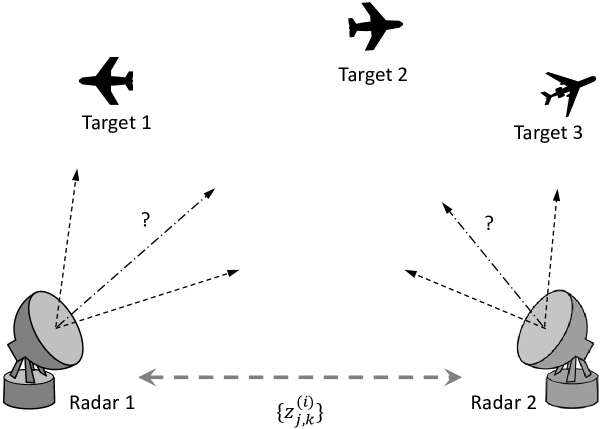
Figure 1: A track selection problem in multi-target tracking.

II Brief preliminaries on game theory

In this section, we provide notation and recall some formal definitions and solution concepts related to game theory that will be used throughout the paper. The focus is put on noncooperative game theory, the dominant branch of game theory, and specifically on so-called normal-form games [24].

Definition 1.

A finite, $N$-person normal-form game is a tuple $\Gamma=(\mathcal{N},\mathcal{S},u)$, where:

• $\mathcal{N}$ is a finite set of $N$ players.

• $\mathcal{S}=\mathcal{S}_{1}\times\cdots\times\mathcal{S}_{N}$, where $\mathcal{S}_{i}$ is a finite set of actions (strategies) available to player $i$, $\forall i\in\mathcal{N}$. Each vector $s=(s_{1},\ldots,s_{N})\in\mathcal{S}$ is called an action (strategy) profile.

• $u=(u_{1},\ldots,u_{N})$ where $u_{i}\colon\mathcal{S}\rightarrow\mathbb{R}$ is a real-valued utility (or payoff) function for player $i$, $\forall i\in\mathcal{N}$ .

To reason about multiplayer games, one can rely on solution concepts, i.e., principles according to which interesting outcomes of a game can be identified. Some fundamental concepts, which will be used throughout this paper, are described in the sequel. A basic and the most widely accepted one is the celebrated Nash equilibrium. Formally, in case where players make deterministic choices (pure strategies) the Nash equilibrium is defined as follows [24].

Definition 2.

A strategy profile $s=(s_{1},\ldots,s_{N})$ is a pure-strategy Nash equilibrium if, for all players $i$ and for all strategies $s^{\prime}_{i}\neq s_{i}$, it holds that

$$u_{i}(s_{i},s_{-i})\geq u_{i}(s^{\prime}_{i},s_{-i}),$$

where $s_{-i}=(s_{1},\ldots,s_{i-1},s_{i+1},\ldots,s_{N})$ is defined as a strategy profile $s$ without player $i$’s strategy.

Otherwise stated, a Nash equilibrium (NE) is a state of a non-cooperative game where no player can unilaterally improve its utility by taking a different strategy, if the other players remain constant in their strategies.

Next, we define the concepts of Pareto domination and Pareto optimality.

Definition 3.

Strategy profile $s$ Pareto dominates strategy profile $s^{\prime}$ if $\forall i\in\mathcal{N}$, $u_{i}(s)\geq u_{i}(s^{\prime})$, and there exists some $j\in\mathcal{N}$ for which $u_{j}(s)>u_{j}(s^{\prime})$. Also, strategy profile $s$ is Pareto optimal if there does not exist another strategy profile $s^{\prime}\in\mathcal{S}$ that Pareto dominates $s$.

To evaluate the (in)efficiency of NE there is a notion called the price of anarchy, which is defined as the ratio of a centralized solution to the worst-case equilibrium in terms of the utility sum that is in economics literature known as ”social welfare”.

Definition 4.

The price of anarchy (PoA) is given as

$${\rm PoA}={\max\limits_{s\in\mathcal{S}}\,\,\sum_{i\in\mathcal{N}}u_{i}(s)\over\min\limits_{s\in\mathcal{S}^{\rm NE}}\,\,\sum_{i\in\mathcal{N}}u_{i}(s)}\,,$$

where $\mathcal{S}^{\rm NE}$ is the set of Nash equilibria of the game.

Note that in case where the equilibria are fully efficient, the PoA is equal to 1.

Finally, we define the notion of correlated equilibrium, which is a generalization of Nash equilibrium [43], [44].

Definition 5.

A correlated equilibrium consists of a probability vector $\pi$ on $\mathcal{S}$ such that the following is satisfied, $\forall i\in\mathcal{N}$ and $\forall s_{i},s^{\prime}_{i}\in\mathcal{S}_{i}$:

$$\sum\limits_{s_{-i}\in\mathcal{S}_{-i}}\pi(s_{i},s_{-i})[u_{i}(s_{i},s_{-i})-u_{i}(s_{i}^{\prime},s_{-i})]\geq 0.$$

To interpret the inequality above, let us first divide it by the marginal probability $\pi(s_{i})$, which yields:

$$\sum\limits_{s_{-i}\in\mathcal{S}_{-i}}\pi(s_{-i}|s_{i})[u_{i}(s_{i},s_{-i})-u_{i}(s_{i}^{\prime},s_{-i})]\geq 0.$$

Thus, an intuitive interpretation of correlated equilibrium is as follows: Suppose that a strategy profile $s\in\mathcal{S}$ is chosen at random, e.g., by some virtual referee, according to the joint distribution $\pi$. Each player $i$ is then given, by the ”referee”, its own recommendation $s_{i}$. The inequality above means that player $i$ cannot obtain a higher expected utility by selecting strategy $s_{i}^{\prime}$ instead of the ”recommended” one, i.e., $s_{i}$. Also, in every finite game, the set of correlated equilibria is nonempty, closed and convex.

III Problem formulation section

Let us consider a network of MFR radars which aims at tracking several targets, e.g., see Fig. 1. Let $\mathcal{N}$ denote the set of $N$ radars and $\mathcal{T}$ denote the set of $T$ targets. We consider that the position of each radar node $i\in\mathcal{N}$ is known. Although there are works in the tracking literature that consider unknown number of targets, e.g., [6], [7], in this work we focus on the case where the number of targets at each time instant is known. The current positions of targets are assumed to be known approximately. Also, the targets are supposed to be well-separated; thus the data association problem is trivial and different transmission beams are required so as to illuminate distinct targets. Furthermore, assume that there is no central processing node to perform track filtering; in other words, fusion is done at each radar node.

Next, the dynamics of each target $j\in\mathcal{T}$, at each discrete time $k$, are represented using the so-called white noise constant velocity model [4], [17] given by

$$\mathrm{x}_{j,k} =F\cdot\mathrm{x}_{j,k-1}+w_{j,k-1}$$ (1)

$$z_{j,k}^{(i)} =h^{(i)}_{j}(\mathrm{x}_{j,k})+\nu^{(i)}_{j,k}$$ (2)

where

• the state vector $\mathrm{x}$ for each target $j$ is comprised of the two dimensional coordinates and velocity, i.e., $\mathrm{x}_{j}=[x_{j},y_{j},v_{j,x},v_{j,y}]^{T}$ where $[\cdot]^{T}$ stands for the transposition of the argument,

• $F$ is a $4\times 4$ matrix corresponding to the deterministic target dynamics given as

  $$F=\left[\begin{smallmatrix}1&t_{u}\\ 0&1\end{smallmatrix}\right]\otimes I_{2}$$ (3)

  with $\otimes$ being the Kronecker product, $I_{2}$ stands for a $2\times 2$ identity matrix and $t_{u}$ is the update time that is fixed,

• the process noise $w$ is Gaussian with zero mean and covariance

  $$Q=\sigma^{2}_{w}\cdot\left[\begin{smallmatrix}t_{u}^{3}/3&t_{u}^{2}/2\\ t_{u}^{2}/2&t_{u}\end{smallmatrix}\right]\otimes I_{2}$$ (4)

  where $\sigma^{2}_{w}$ models maneuverability,

• the measurement vector $z_{j,k}^{(i)}$, at each radar $i\in\mathcal{N}$, consists of range and azimuth, i.e., $z_{j,k}^{(i)}=\left[r_{j,k}^{(i)},a_{j,k}^{(i)}\right]^{T}$,

• the nonlinear transformation $h^{(i)}_{j}(\mathrm{x}_{j})$ is given by

  $$h^{(i)}_{j}(\mathrm{x}_{j})=\begin{bmatrix}\sqrt{(x_{j}-x_{i})^{2}+(y_{j}-y_{i})^{2}}\\ \mathrm{arctan}((y_{j}-y_{i})/(x_{j}-x_{i}))\end{bmatrix},$$ (5)

• the measurement noise $\nu^{(i)}_{j}$ is zero-mean Gaussian with covariance $R_{j,i}=\mathrm{diag}\left\{[\sigma^{(i)}_{r_{j}}]^{2},[\sigma^{(i)}_{a_{j}}]^{2}\right\}$.

The radars have limited time budget in the sense that they cannot take measurements of all targets during the same time slot. The number of measurements per scan that each radar can make is given by $m<|\mathcal{T}|$. Since there is no central entity that may coordinate actions of the radars, a distributed solution is needed.

Furthermore, radars may experience different target observability conditions; thus, the set of the targets that are observable at each radar $i$ is denoted by $\mathcal{T}_{i}$, and it satisfies $\mathcal{T}_{i}\subseteq\mathcal{T}$. The interaction among the radars is existing but limited to sharing the measurements $\{z_{j,k}^{(i)}\}$ related to the previously selected targets. The communication neighborhood of any particular radar $i$, together with radar $i$, is denoted as $\mathcal{N}_{i}$, where $\mathcal{N}_{i}\subseteq\mathcal{N}$. The number of transmissions each radar $i$ collects from its neighborhood $\mathcal{N}_{i}$, and which are related to some target $j\in\bigcup_{i\in\mathcal{N}_{i}}\mathcal{T}_{i}$, is denoted as $m^{t}_{j}(i)$. For notational simplicity, in the rest of this section we drop the index $j$ for targets where no confusion is possible.

At each radar $i$ and for each target $j$, the tracking process is performed by an Extended-Kalman Filter (EKF). Firstly, the prediction step occurs, i.e.,

$$\mathrm{x}_{k|k-1} =F\cdot\mathrm{x}_{k-1|k-1}$$ (6)

$$P_{k|k-1} =FP_{k-1|k-1}F^{T}+Q$$ (7)

where $\mathrm{x}_{k|k-1}$ and $P_{k|k-1}$ are the state estimate and the error covariance matrix for time step $k$ given all measurements till time step $k-1$. Then, the updating step takes place where each available measurement for target $j$ of some radar $n\in\mathcal{N}$ is used in a cyclic manner. In particular, for each $p\in\{1,\ldots,m_{j}^{t}(n)\}$,

$$K_{k}^{(p)} =P_{k|k}^{(p-1)}[H^{(p)}_{k,n}]^{T}\left(H^{(p)}_{k,n}P_{k|k}^{(p-1)}[H^{(p)}_{k,n}]^{T}+R_{n}\right)^{-1}$$ (8)

$$\mathrm{x}_{k|k}^{(p)} =\mathrm{x}_{k|k}^{(p-1)}+K_{k}^{(p)}\left(z_{k}^{(n)}-h^{(n)}\left(\mathrm{x}_{k|k}^{(p-1)}\right)\right)$$ (9)

$$P_{k|k}^{(p)} =\left(I-K_{k}^{(p)}H^{(p)}_{k,n}\right)P_{k|k}^{(p-1)}$$ (10)

where $P_{k|k}^{(p)}$ denotes the error covariance matrix after $p$ incremental updates at the same time step $k$, with $P_{k|k}^{(0)}=P_{k|k-1}$ and $\mathrm{x}_{k|k}^{(0)}=\mathrm{x}_{k|k-1}$. The linearized measurement matrix of radar $n$ at time $k$ is $H^{(p)}_{k,n}=\partial h^{(n)}/\partial\mathrm{x}$ evaluated at $\mathrm{x}_{k|k}^{(p-1)}$. Note that, due to the fact that the coordinates $(x_{n},y_{n})$ of each radar $n\in\mathcal{N}$ are known, the radars do not need to exchange $\{H_{k,n}\}$ matrices in order to implement the algorithm above.

In the following, we study a natural game theoretic variant of this problem. Specifically, we assume that the radars are autonomous decision-makers interested in optimizing their own tracking performance. In other words, the selections of each radar are autonomous in the sense that there is no entity to tell radars what to do in a hierarchical type of structure, nor is there any negotiation among radars. We analyze two indicative scenarios with respect to the observability conditions, communication topology as well as the radars’ interests:

• Scenario 1: a scenario where each radar $i$ observes all targets, i.e., $\bigcap_{i\in\mathcal{N}}\mathcal{T}_{i}=\mathcal{T}$, communicates with all neighbors (all radars communicate through the full graph), i.e., $\mathcal{N}_{i}=\mathcal{N}$, and is interested in tracking all targets in $\mathcal{T}$ (all targets have the same importance).

• Scenario 2: a more general scenario where the radars do not necessarily have the same target interests and where the observability and communication equalities above (full observability and full connectivity conditions) do not need to hold, i.e., $\exists i\in\mathcal{N}\mid\mathcal{N}_{i}\subset\mathcal{N}\lor\mathcal{T}_{i}\subset\mathcal{T}$.

For both scenarios, the fact that each radar (or the radar operator) autonomously and rationally decides to track the targets that increase its utility can be modeled as a one-stage non-cooperative game in normal form, which is the most fundamental representation type in game theory [24]. In following two sections, we analyze the track selection problem in each scenario separately.

IV Scenario 1: the problem of coordination

Firstly, note that there are many classes of normal-form games; however, due to the particularities of the scenario considered, in this section we focus on coordination games, which do not rest solely upon conflict among players. Instead, as their name suggests, more emphasis is put on the coordination issue where players may have an incentive to conform with or to differ from what others do. In the latter case, this kind of games are usually called anti-coordination games [24], [45]-[46].

IV-A Game-theoretic model

We assume that the players are rational and their objective is to maximize their payoff, i.e., the tracking accuracy of all targets. Formally, the track selection game $\Gamma^{(1)}=(\mathcal{N},\mathcal{S},u)$ has the subsequent components:

• The players are the radars represented by the set $\mathcal{N}$.

• The strategy of each radar $i$ is represented by a $T$-tuple $s_{i}=(s_{i,1},s_{i,2},\ldots,s_{i,T})$ where $s_{i,j}=a$ if radar $i$ devotes $a$ transmission beams to a target $j$, with $a\leq m$. Each strategy-tuple has at most $m$ transmissions, i.e., $\sum_{j=1}^{T}s_{i,j}\leq m$. Also, note that

  $$m^{t}_{j}(i)=m^{t}_{j}=\sum_{i=1}^{N}s_{i,j}.$$

• The utility for each radar $i$ is given by

  $$\begin{split}u_{i}(s_{i},s_{-i})=\sum_{j=1}^{T}\mathrm{gain}_{j}(m^{t}_{j})\,,\end{split}$$ (11)

  where the term $\mathrm{gain}_{j}(m^{t}_{j})$ represents the tracking accuracy gain for target $j\in\mathcal{T}$ and it is defined by

  $$\mathrm{gain}_{j}(m^{t}_{j})=\mathrm{Tr}\left\{P_{j,k|k-1}-P_{j,k|k}^{(m^{t}_{j})}\right\}$$ (12)

  where $\mathrm{Tr}\{\cdot\}$ stands for the trace operator and all radars are assumed to have the same initial guesses $\mathrm{x}_{j,0|0}$ and $P_{j,0|0}$.

In other words, the strategy of radar $i$ defines the number of transmissions per each target, at a given time slot, see Fig. 2. Due to the fact that radars share their measurements, their tracking accuracy gains for a specific target are dependent on all radars’ measurements related to that target.

Figure 2: An example strategy profile displayed as a matrix, for $\mathcal{T}=\{a,\ldots,e\}$, and $|\mathcal{N}|=m=3$.

Figure 3: An example of a track allocation in terms of gains per target where $\mathcal{T}=\{a,\ldots,e\}$, and $|\mathcal{N}|=m=3$. Each box represents a gain increment due to a measurement, and the number of measurements per target, $m^{t}_{j}$, varies between 1 and 4 across targets in $\mathcal{T}$. In case 3, the gains are equal for the same number of measurements, while in case 3 they differ.

Note that the gain in (12) can be expressed as

$$\mathrm{gain}_{j}\left(m^{t}_{j}\right)=\sum_{p=1}^{m^{t}_{j}}\Delta g^{(j)}_{p},$$ (13)

where

$$\Delta g^{(j)}_{p}=\mathrm{Tr}\{P_{j,k|k}^{(p-1)}-P_{j,k|k}^{(p)}\}$$ (14)

and $\Delta g^{(j)}_{1}=\mathrm{gain}_{j}(1)$. To analyze the proposed game, we proceed by adopting the following practical assumptions, for all $j\in\mathcal{T}$ and $p\in\{1,\ldots,m^{t}_{j}\}$:

• Assumption 1: the gain function in (12) is increasing in the number of measurements, i.e., $\Delta g^{(j)}_{p}>0$,

• Assumption 2: estimation accuracy gain increment $\Delta g^{(j)}_{p}$ decreases as the order of measurements $p$ grows, i.e., $\Delta g^{(j)}_{p}>\Delta g^{(j)}_{p+1}$.

Finally, the following two cases are analyzed:

• $\Delta g^{(j)}_{p}=\Delta g_{p}$, for all $j\in\mathcal{T}$ and $p\in\{1,\ldots,m^{t}_{j}\}$

• $\Delta g^{(j)}_{p}\neq\Delta g^{(\ell)}_{p}$, for $j\neq\ell$, and $\mathrm{min}_{j\in\mathcal{T}}\Delta g^{(j)}_{p}>\mathrm{max}_{j\in\mathcal{T}}\Delta g^{(j)}_{p+1}$.

Case a) represents an idealistic case where all nodes would have very similar measurements among themselves and related to all targets, see Fig 33. A more realistic scenario, corresponding to case b), is illustrated in Fig 33. In the next subsection, we characterize the Nash equilibria of the aforementioned cases.

IV-B Nash equilibria

Generally, in a coordination game, there are multiple NE. If the players have the same payoffs, and the equilibria are equal, the game is a pure coordination one. In fact, in such a game, all NE are Pareto optimal. On the other hand, in a ranked one, the NE differ and usually there is only one Pareto optimal equilibrium [47].

Now, the main findings related to the NE for cases (a) and (b) are provided.

Proposition 1.

The game for case (a) has PoA $=1$, and any track assignment is a Nash equilibrium, if $\sum_{j=1}^{T}s_{i,j}=m$, and if

• $m^{t}_{j}\leq 1$, $\forall j\in\mathcal{T}$, for a scenario where $N\cdot m\leq T$

• $\mathrm{max}_{j,\ell\in\mathcal{T}}\{|m^{t}_{j}-m^{t}_{\ell}|\}\leq 1$, $\forall j,\ell\in\mathcal{T}$, for a scenario where $N\cdot m>T$.

Proof.

Firstly, let us assume that there is a radar $i$ such that $\sum_{j=1}^{T}s_{i,j}<m$ and that the corresponding $s^{\ast}$ is an NE. Then, radar $i$ can change its strategy by taking an additional measurement. Due to the fact that the radar’s gain function in (12) is increasing in the number of measurements, its utility will be increased. But that contradicts our initial assumption that $s^{\ast}$ is an NE; thus, as per our intuition, each radar should make all possible transmissions toward the target(s) at each time instant. Next, note that if the total number of measurements is less than or equal to the number of targets, the radars are worse off if more than one measurement in total is devoted to the same target. Also, due to the structure of gain function, NE are precisely $\frac{T!}{\left(T-N\cdot m\right)!}$ outcomes in which each measurement is devoted to a distinct target. On the other hand, if $N\cdot m>T$, the corresponding condition states that all targets should be covered as equally as possible. Here, each NE corresponds to a balanced allocation. For instance, the allocation in Fig 33 is not an NE since the payoffs can be increased if some player moves its measurement from target $b$ to any other target. Finally, since the gain of any target is the same for the same number of measurements, the game appears to be a pure anti-coordination one. Thus, every NE is also Pareto optimal, which finally implies that PoA=1. ∎

Proposition 2.

The game for case (b) has PoA $>1$, and any track assignment is an NE, if $\sum_{j=1}^{T}s_{i,j}=m$, and if,

• for a scenario with $N\cdot m\leq T$, each radar chooses its most accurate target that has not been selected,

• for $N\cdot m>T$, the first $\left\lceil{\frac{N\cdot m}{T}}\right\rceil-1$ levels are filled in, i.e., $m_{j}^{t}\geq\left\lceil{\frac{N\cdot m}{T}}\right\rceil-1$, $\forall j\in\mathcal{T}$, and for the $\left\lceil{\frac{N\cdot m}{T}}\right\rceil$-th level each radar chooses its most accurate target that has not been selected by others, where $\lceil{\cdot}\rceil$ is the ceiling function.

Proof.

Similar arguments hold as for Prop. 1. Yet, the game above seems to be a ranked anti-coordination game. Note that here there are still multiple NE, but not all NE are necessarily equal, and hence, not every NE is Pareto optimal (only one is). So, the conditions above are not sufficient to have also a Pareto optimal NE, and consequently, PoA is strictly greater than 1. ∎

IV-C BRD-based distributed track selection algorithm

In the sequel, we present a simple, low-complexity, distributed algorithm, based on the best-response dynamics (BRD) [24], [26], [27] literature, that looks for the NE of the analyzed game. Toward this goal, let us first define the notion of radar $i$’s best response to the vector of strategies $s_{-i}$, denoted by $\mathrm{BR}_{i}(s_{-i})$, as the set-valued function

$$\mathrm{BR}_{i}(s_{-i})=\mathrm{arg}\,\max\limits_{s_{i}\in\mathcal{S}_{i}}u_{i}(s_{i},s_{-i}).$$

Note that there are two versions of BRD that can be used; namely, the sequential version

$$s_{i}(k+1)\in\mathrm{BR}_{i}\big{(}s_{1}(k+1),\ldots\hskip 113.81102pt$$

$$\ldots,s_{i-1}(k+1),s_{i+1}(k),\ldots,s_{N}(k)\big{)},$$

where $s_{i}(k+1)$ is the action selected by radar $i$ at time step $(k+1)$, and the simultaneous one where all players update their actions synchronously

$$s_{i}(k+1)\in\mathrm{BR}_{i}\left(s_{-i}(k)\right).$$

Although the former one is more frequently used [27], it requires the definition of a cyclic path that covers all nodes, which is an NP-hard problem [48], [49], and furthermore it has limited applicability in large and delay-intolerant networks if the whole cycle has to be performed at each time instant. Thus, we focus on the simultaneous BRD implementation which, on the other hand, may experience the problem of a coordination failure due to strategic uncertainty (see Fig. 4). Nevertheless, this problem can be alleviated if radars select their best responses with some probability $\alpha<1$.

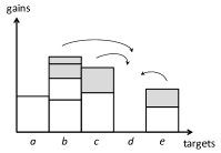
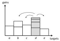
Figure 4: A coordination failure example; 4 initial track allocation; 4 four radars decide to change their current track choices (gray boxes) and illuminate target $d$; 4 the track allocation in the following time instant and possible radar choices (denoted by the arrows) that may result into the cyclic behavior.

In the games above where $N\cdot m>T$, in general, two types of NE may arise, one where a radar illuminates only different targets and the other where it chooses the same target more than once. In practice, it is of interest to exploit the radars’ diversity; thus, we focus on the former type. Let $\mathcal{T}_{\mathrm{sel}}^{(i)}$ denote the set of targets selected by radar $i$.

Then, a summary of the proposed algorithm is provided in the following.

 
Algorithm 1: Low-complexity BRD-based distributed scheme (LC-BRD) for track selection
 

• Start with any strategy profile $s(0)$.

• At each time instant $k=1,2,\ldots,$ each radar $i\in\mathcal{N}$ performs the following steps:

  • Count $m_{j}^{t}$, $\forall j\in\mathcal{T}$, and reallocate the measurements for $\forall j\in\mathcal{T}_{\mathrm{sel}}^{(i)}$ satisfying $s_{i,j}>1$ to a target $\mathrm{argmin}_{\ell\in\{\mathcal{T}\setminus\mathcal{T}_{\mathrm{sel}}^{(i)}\}}m_{\ell}^{t}$.

  • With probability $\alpha$, reallocate the measurement from target $j$ to $\ell$ until

    • $\exists j\in\mathcal{T}_{\mathrm{sel}}^{(i)}$ such that $m_{j}^{t}>\left\lceil{\frac{N\cdot m}{T}}\right\rceil$ and the measurement for $\ell$ is the most accurate one of those satisfying $\mathrm{argmin}_{q\in\{\mathcal{T}\setminus\mathcal{T}_{\mathrm{sel}}^{(i)}\}}m_{q}^{t}$, or

    • $m_{j}^{t}-m_{\ell}^{t}=1$, where $m_{j}^{t}=\mathrm{max}_{q\in\mathcal{T}_{\mathrm{sel}}^{(i)}}m_{q}^{t}$ and $m_{\ell}^{t}=\mathrm{min}_{q\in\{\mathcal{T}\setminus\mathcal{T}_{\mathrm{sel}}^{(i)}\}}m_{q}^{t}$, and if measurement for $\ell$ is more accurate than the one for $j$.

  • Transmit/receive measurements, and $\forall j\in\mathcal{T}$, execute (6)-(7) and employ all available measurements in (8)-(10).

  • (optional) if $u_{i}\big{(}s_{i}(k),s_{-i}(k)\big{)}<u_{i}\big{(}s_{i}(k-1),s_{-i}(k-1)\big{)}$ revert back to the strategy from $k-1$ and skip the first 2 steps, i.e., $s_{i}(k+1)=s_{i}(k-1)$.

 

In the context of general BRD algorithms, players need to observe the actions played by the others; however, in our algorithm, it can be verified that the knowledge of the numbers of transmissions per each target $j$, i.e., $\left\{m^{t}_{j}\right\}_{j=1}^{T}$, is sufficient. Specifically, note that $\left\{m^{t}_{j}\right\}_{j=1}^{T}$ are aggregate functions of the radars’ actions and, due to $u_{i}(s_{i},s_{-i})=u_{i}(m^{t}_{1},\ldots,m^{t}_{T})$, observing the actions themselves is not necessary.

Note that there are no convergence results for general games using BRD, i.e., a BRD-based algorithm may miss an NE [24], [27]. Fortunately, for some special classes of games there exist sufficient conditions under which the convergence of the sequential BRD to a pure NE is always guaranteed. For instance, one such class is related to the so-called potential games [50], which we define next.

Definition 6.

A finite, $N$-person normal-form game $\Gamma=(\mathcal{N},\mathcal{S},u)$ is called a potential game if there exists a function $\Phi\colon\mathcal{S}\rightarrow\mathbb{R}$ such that $\forall i\in\mathcal{N}$ and for all $(s_{i},s_{-i}),(s^{\prime}_{i},s_{-i})\in\mathcal{S}:$

$$u_{i}(s_{i},s_{-i})-u_{i}(s^{\prime}_{i},s_{-i})=\Phi(s_{i},s_{-i})-\Phi(s^{\prime}_{i},s_{-i}),$$

and such a function $\Phi$ is called potential function of the game.

In every finite potential game, every improvement path is finite. Since a finite game has a finite strategy space, the potential function takes on finitely many values and the above sequence must terminate in finitely many steps in an equilibrium point.

Unlike the sequential BRD, there does not seem to exist general convergence results for the simultaneous BRD, yet only a few application-specific proofs[27]. Nevertheless, the proposed Algorithm $1$ does converge to a pure NE.

Theorem 1.

The proposed Algorithm 1, with the s4) step, does converge to a pure Nash equilibrium of the proposed one-shot track selection game $\Gamma^{(1)}=(\mathcal{N},\mathcal{S},u)$, defined in Sec IV-A.

Proof.

Let us first analyze a hypothetical, sequential version of the proposed algorithm. Note that one may construct a potential function $\Phi$ for the analyzed game, i.e., by setting $\Phi=u_{i}(s)$, $\forall i\in\mathcal{N}$. Thus, a sequential BRD-based strategy for the analyzed game would converge. Now, for the proposed (simultaneous) algorithm, note that in general case $\Phi$ is not non-decreasing as time progresses; however, due to the s4) step, only the states where $\Phi$ is not smaller than the best previous $\Phi$ value are actually kept. Specifically, in case where the players at time $k$ select a coordination failure profile which may result in $\Phi(k)<\Phi(k-1)$ (such as one given in Fig. 4), this step ensures that $\Phi(k+1)=\Phi(k-1)$. Then, due to $\alpha<1$, there is a non-negligible probability that only one player will update (as in the asynchronous version) and $\Phi$ will increase; thus, the algorithm will eventually converge. ∎

Remark 1: Strictly speaking, the proposed algorithm with the s4) step is not a traditional simultaneous BRD, since it requires that each player also stores in memory the action and the utility value from the previous time step. This additional, yet small memory requirement is sufficient but not necessary for the algorithm to converge. For properly set $\alpha$, our simulations have shown that the proposed algorithm, even without the s4) step, actually converges and performs well (see also [42]).

Dynamic scenario: Note that the tracking accuracy gain in (12), which constitutes the utility of each radar in (11), generally depends on measurement noise covariance $R_{j,i}$, deterministic target dynamics $F$ and process noise covariance $Q$. To account for time-varying accuracy measures, i.e., range and azimuth variances, and to deal with possibly high target dynamics, the proposed algorithm can be modified in one of the following ways:

• LC-BRD algorithm can be repeated every $K$ time instants so as to search for other NE during the tracking process, or

• Each radar running LC-BRD may randomly change its strategy in step $s2$ (regardless of the conditions in this step) with a small $\epsilon$ probability. In other words, step $s2$ in LC-BRD is run with probability $1-\epsilon$.

The modifications above achieve similar performance, as it will be shown in the simulation section.

V Scenario 2: Coordination $\&$ Conflict

In the previous section, we have analyzed the scenario where all radars share the same interests; thus, the main challenge has been to tackle the problem of coordination among radars. Note that, in practice, different radars or groups of radars (or more precisely, radar operators) can have different interests over targets. For instance, the radar operators can have different target priorities. Or even simpler, radar operators can be interested only in a specific region and/or in a specific type of targets. Yet, in such situations it is still important to exploit the network cooperation, as in the scenario analyzed in the previous section. Thus, here we focus on a more demanding scenario where radars may have different interests and where issues of conflict may also arise. Specifically, we assume that radars:

• do not necessarily have the same target interests,

• are limited to partial target observability, and

• do not communicate with all other radars.

An example of such a scenario is depicted in Fig. 5. For instance, radar $1$ in Fig. 5, denoted as $R_{1}$, communicates with only two neighboring radars ($R_{2}$ and $R_{3}$), observes only two targets ($T_{1}$ and $T_{2}$), while being interested in tracking three targets ($T_{1}$-$T_{3}$), i.e., there are three non-zero weights, which correspond to $T_{1}$-$T_{3}$, in its weight vector $w_{1}$. On the other hand, $R_{3}$ has different yet overlapped interests and different neighbors and observability conditions.

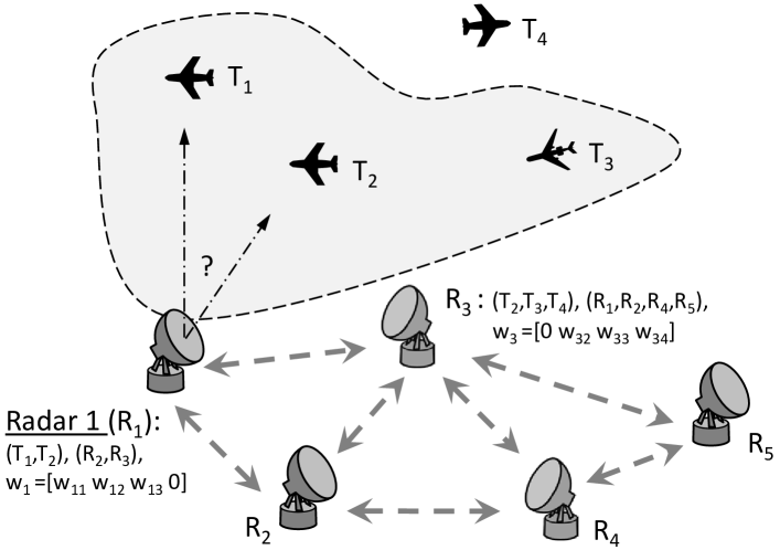
Figure 5: A track selection problem in a scenario with partial observability, limited communication and different interests among radars.

V-A Game-theoretic model

Here, we redefine the track selection game $\Gamma^{(2)}=(\mathcal{N},\mathcal{S},u)$ as:

• The players are the radars represented by the set $\mathcal{N}$.

• The strategy of each radar $i$ is represented by a $T$-tuple $s_{i}=(s_{i,1},s_{i,2},\ldots,s_{i,T})$ where

  $$s_{i,j}=\begin{cases}a,&\text{if }j\in\mathcal{T}_{i}\\ 0,&\text{otherwise}\end{cases}$$ (15)

  where $a$ is the number of transmission beams that radar $i$ devotes to target $j\in\mathcal{T}_{i}$ and it holds that $a\leq m$. Each strategy-tuple has at most $m$ transmissions, i.e., $\sum_{j\in\mathcal{T}_{i}}s_{i,j}\leq m$. Now, the number of transmissions each radar $i$ collects from $\mathcal{N}_{i}$ and related to some target $j\in\bigcup_{i\in\mathcal{N}_{i}}\mathcal{T}_{i}$ is given as $m^{t}_{j}(i)=\sum_{i\in\mathcal{N}_{i}}s_{i,j}$.

• The utility for each radar $i$ is given by

  $$\begin{split}u_{i}(s_{i},s_{-i})=\sum_{j=1}^{T}w_{i,j}\cdot\mathrm{gain}_{j}\left(m^{t}_{j}(i)\right)\,,\end{split}$$ (16)

  with $\mathrm{gain}_{j}\left(m^{t}_{j}(i)\right)=\mathrm{Tr}\left\{P_{j,k|k-1}-P_{j,k|k}^{(m^{t}_{j}(i))}\right\}$, and $w_{i,j}$ being the weight that a radar $i$ gives to some target $j$. In fact, $w_{i,j}$ can be seen as $(i,j)^{\mathrm{th}}$ element of $N\times T$ matrix $W$ which defines the target interests across all radars. Also, note that $u_{i}(s_{i},s_{-i})=u_{i}\left(\{s_{l}\}_{l\in\mathcal{N}_{i}}\right)$.

V-B Correlated equilibria and regret-matching

The scenario considered in the previous example resembles the well-known Battle of the Sexes game [24] where players have a common interest to coordinate (or in our case to anti-coordinate), but they have different preferences regarding the (anti-)coordinated states of the game (which are NE). However, for a general setting of our game defined above, it is not easy to characterize possible NE neither in terms of their efficiency nor even their existence. Furthermore, we cannot ensure that the game is potential. This is due to the fact that, in general case, it is difficult to construct a potential function $\Phi$ since an action profile change can influence different players in an arbitrarily different way (see an example in Fig. 6).

(a) $R_{1}$, time $k$

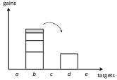
(b) $R_{3}$, time $k$

(c) $R_{1}$, time $k+1$

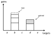
(d) $R_{3}$, time $k+1$

Figure 6: Assume a track allocation across the network as in Fig. 3. Due to limited connectivity and different interests, at time $k$, radar 1 ($R_{1}$) experiences the gains given in 6(a), and those in 6(b) are for radar 3 ($R_{3}$) which decides to change its selection. At time $k+1$, $R_{1}$ has a (great) loss while $R_{3}$ has a (relatively small) gain.

Remark 2: In the extreme case where radars have totally different interests (with no overlap w.r.t. the interests and communication topology), then it would be easy to define a potential function (just the sum of all utilities). However, the solution (NE) is trivial since the problem is totally decoupled (there is no inter-dependence); each radar’s utility depends only on its own strategy selection $u_{i}(s)=u_{i}(s_{i}),\forall i\in\mathcal{N}$.

For the reasons mentioned above, here we focus on the solution concept of correlated equilibrium (CE). Note first that, as mentioned in Sec. II, a CE always exists in a finite game [44]. Actually, every NE is a CE and NE correspond to the special case of a CE for which the joint distribution over the strategy profiles $\pi(s_{i},s_{-i})$ factorizes as the product of its marginals, i.e., the play of different players is independent [43], [44]. Furthermore, in certain settings the set of CE may include even the distribution that is not in the convex hull of the NE distributions.

Next, we will exploit a class of simple, adaptive algorithms, called regret matching, in order to reach a CE of the analyzed track selection game. It does not entail any sophisticated updating, prediction, or fully rational behavior [51]. The approach can be summarized as follows: At each time instant, a radar may either continue playing the same target strategy as in the previous time instant, or switch to other strategies, with probabilities that are proportional to how much higher his accumulated accuracy gain would have been had he always made that change in the past. Specifically, at each time instant $k$ and for any two distinct strategies $s_{i}^{\prime}\neq s_{i}$, the regret which radar $i$ experiences at time $k$ for not playing $s_{i}^{\prime}$ is given by

$$\begin{split}R_{i,k}(s_{i},s_{i}^{\prime})=\max\{D_{i,k}(s_{i},s_{i}^{\prime}),0\},\end{split}$$ (17)

where the term $D_{i,k}(s_{i},s_{i}^{\prime})$ represents the average payoff at time $k$ for not having played, every time that $s_{i}$ was played in the past $k_{p}\leq k$, the different strategy $s_{i}^{\prime}$:

$$\begin{split}&D_{i,k}(s_{i},s_{i}^{\prime})=\\ &\qquad={1\over k}\sum\limits_{k_{p}\leq k}\left[u_{i}\left(s_{i}^{\prime}(k_{p}),s_{-i}(k_{p})\right)-u_{i}\left(s_{i}(k_{p}),s_{-i}(k_{p})\right)\right].\end{split}$$ (18)

Next, the probability at time $k+1$ for radar $i$ to play some strategy $s_{i}^{\prime}\in\mathcal{S}_{i}$ is a linear function of its regret vector, i.e.,

$$\begin{split}\begin{cases}\pi^{k+1}_{i}(s_{i}^{\prime})=\frac{1}{\mu}R_{i,k}(s_{i},s_{i}^{\prime}),\quad\text{for all}\,\,s_{i}^{\prime}\neq s_{i},\\ \pi^{k+1}_{i}(s_{i})=1-\sum\nolimits_{s_{i}^{\prime}\neq s_{i}}\pi^{k+1}_{i}(s_{i}^{\prime}),\quad\text{otherwise},\end{cases}\end{split}$$ (19)

where the fixed constant $\mu>0$ is selected to be large enough such that $\pi^{k+1}_{i}(s_{i})>0$. Finally, for every $k$, we define the empirical distribution $\eta_{k}$ of the strategy profiles played up to time $k$, i.e., for each $s\in\mathcal{S}$,

$$\begin{split}\eta_{k}(s)={1\over k}\#\{k_{p}\leq k:s(k_{p})=s\},\end{split}$$ (20)

with $\#(\cdot)$ standing for the number of times the event inside the brackets occurs while $s(k_{p})$ is the action profile played at time $k_{p}$.

Theorem 2.

If every radar select targets according to (19), then the empirical distributions $\eta_{k}$ converge almost surely as $k\rightarrow\infty$ to the set of correlated equilibrium distributions of the game $\Gamma^{(2)}$.

Proof.

For the proof, see [51]. ∎

Dynamic scenario: Due to possibly time-varying accuracy measures and high target dynamics, as explained in the end of Sec. IV-C, as well as time-varying radar interests, the suggested approach has to be modified so as to take into account the aforementioned effects. In fact, by incorporating an adaptive mechanism in the calculation of the average regret, it can be shown that the resulting algorithm can track the changes if they are sufficiently small.

Firstly, note that the average regret in (18) can be computed recursively, i.e.,

$$\begin{split}D_{i,k}(s_{i},s_{i}^{\prime})=&{k-1\over k}\,D_{i,k-1}(s_{i},s_{i}^{\prime})+\\ &+{1\over k}\left[u_{i}\left(s_{i}^{\prime}(k),s_{-i}(k)\right)-u_{i}\left(s_{i}(k),s_{-i}(k)\right)\right].\end{split}$$ (21)

Also, the average regret in (18) and (21) exploits the history of all past selections. This is not desirable due to the fact that the tracking accuracy gains slightly change in time due to the aforementioned effects. Thus, to compute the average regret, each radar should exponentially discount the influence of its past selections. Specifically, similarly to [52], we rewrite the average regret recursion as:

$$\begin{split}D_{i,k}(s_{i},s_{i}^{\prime})=&D_{i,k-1}(s_{i},s_{i}^{\prime})\\ &+\theta_{k}\Big{[}u_{i}\left(s_{i}^{\prime}(k),s_{-i}(k)\right)-u_{i}\left(s_{i}(k),s_{-i}(k)\right)\\ &\hskip 108.12054pt-D_{i,k-1}(s_{i},s_{i}^{\prime})\Big{]}.\end{split}$$ (22)

where $\theta_{k}$ is a positive step-size. In case where the step-size $\theta_{k}$ is decreasing with time, the algorithm will converge with probability 1 to the correlated equilibria of a static game. In fact, if $\theta_{k}={1\over k}$, then the recursions in (21) and (22) are identical; thus, the convergence arguments from [51] directly apply. However, for the decreasing step-size, the algorithm may not adapt to the changes caused by the target dynamics. On the other hand, with the fixed step-size $\theta_{k}=\theta$, the algorithm is able to adapt to the changes and can be proved to converge to the set of CE by using the arguments from stochastic averaging theory [53]. For a more detailed discussion, see [52].

Finally, we provide the algorithm based on regret-matching.

 
Algorithm 2: Regret-matching distributed scheme (RM) for track selection
 

• Start with some initial probability vector $\pi^{1}(s)$

• At each time instant $k=1,2,\ldots,$ each radar $i\in\mathcal{N}$ performs the following steps:

  • Select target(s) according to probabilities $\pi^{k}_{i}(s_{i}^{\prime})$ and $\pi^{k}_{i}(s_{i})$ $\forall s_{i}^{\prime}\neq s_{i}$, and denote the selection by $s_{i}$.

  • Calculate $D_{i,k}(s_{i},s_{i}^{\prime})$ using (22).

  • Calculate regret $R_{i,k}(s_{i},s_{i}^{\prime})$ using (17).

  • Find probabilities for the following time instant, i.e., $\pi^{k+1}_{i}(s_{i}^{\prime})$ and $\pi^{k+1}_{i}(s_{i})$ using (19).

 

Computational complexity: It is of interest to comment on the computational complexity of the distributed algorithms proposed in this paper. For illustration only, let us consider that the number of observed targets is the same for all radars, i.e., $|\mathcal{T}_{i}|=|\mathcal{T}_{n}|,\forall i,n\in\mathcal{N}$, and that the radars are interested in all targets that are observable to them. Then, the RM-based algorithm has the complexity that is linear in the number of radars but exponential in $m$, i.e., $\mathcal{O}(N\cdot|\mathcal{T}_{i}|^{m})$. This is in contrast to the centralized approach that can be realized by an exhaustive search and which has the exponential complexity also in the number of radars, i.e., $\mathcal{O}(|\mathcal{T}_{i}|^{N\cdot m})$. On the other hand, note that the LC-BRD proposed in Sec. IV is the most efficient from the computational perspective; its complexity is in the order of $\mathcal{O}(N\cdot m\cdot|\mathcal{T}_{i}|)$.

VI Simulations

In this section, we provide some computer simulations that verify the main findings and demonstrate the effectiveness of the proposed algorithms.

Firstly, we consider an MFR network of $N=3$ radars, each of them making $m=2$ measurements per scan and aiming at tracking $T=5$ targets, see Fig. 7. Specifically, the coordinates of radars are given in Table I. The targets follow white noise constant velocity trajectories with initial $x$, $y$-coordinates and velocities provided in Table II. Initial guesses $\mathrm{x}_{j,0|0}$ are noisy versions of the initial states $\mathrm{x}_{j,0}$ and initial covariances are equal to $P_{j,0|0}=P_{0|0}=\mathrm{diag}\big{\{}(0.1\,km)^{2},\break(0.1\,km)^{2},(0.1\,km/s)^{2},(0.1\,km/s)^{2}\big{\}}$. The update time is $t_{u}=0.25\,s$, and in order to model moderate maneuverability, $\sigma^{2}_{w}$ is set to $2.5\cdot 10^{-5}\,km^{2}/{s^{3}}$. Also, the standard deviation in azimuth is $\sigma^{(i)}_{a_{j}}=\sigma_{a}=2\,mrad$, while the range accuracy varies among the radars and targets as $\sigma^{(i)}_{r_{j}}=b_{i,j}\cdot\sigma_{r}$, where $\sigma_{r}=15\,m$ and coefficient $b_{i,j}$ is taken from the interval $[1,4.5]$.

TABLE I: Radar positions

	$x$ [km]	$y$ [km]
radar 1	-10	0
radar 2	3	0
radar 3	10	0

TABLE II: Target parameters

	$x$ [km]	$y$ [km]	$v_{x}$ [km/s]	$v_{y}$ [km/s]
Target 1	1	6	0.5	0.1
Target 2	0.5	7	0.35	-0.1
Target 3	1.5	3	-0.3	0
Target 4	2	4	-0.2	0.1
Target 5	2.5	5	0.3	0.2

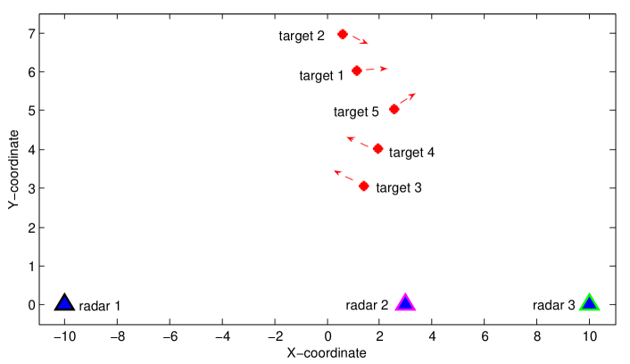
Figure 7: The coordinates of radars and targets.

Most figures present the weighted sum of $\mathrm{Tr}\{P_{j,k|k}^{(m^{t}_{j}(i))}\}$ over all targets and over all radars, i.e.,

$$\begin{split}\sum_{i=1}^{N}\sum_{j=1}^{T}w_{i,j}\cdot\mathrm{Tr}\left\{P_{j,k|k}^{(m^{t}_{j}(i))}\right\},\end{split}$$ (23)

as a function of time $k$. Initially, we focus on the case analyzed in Sec. IV and compare the following strategies:

• Standalone – The standalone radar that does not send/receive measurements. It sequentially chooses $m=2$ different targets each time instant.

• Distributed random with $K=10$ – Distributed strategy where the radars exchange the measurements while each of them randomly selects targets each $K=10$ time instants.

• Distributed random with $K=1$ – Same as in (b), except that targets are being randomly chosen at each time instant, i.e., $K=1$.

• Proposed LC-BRD distributed with $K=10$ – The proposed low-complexity BRD-based distributed algorithm seeking NE while being reinitialized every $K=10$ time instants. The probability $\alpha$ is set to the value of $0.5$.

• Approximated centralized with $K=10$ – The approximated centralized approach based on analytically resolved measurements-to-target allocation every $K=10$ time instants. Due to its exponential search complexity in the total number of measurements, i.e., $\mathcal{O}(T^{N\cdot m})$, the centralized exhaustive search is computationally challenging even for the considered scenario of $T=5$, $N=3$ and $m=2$. For this reason, the coefficients in noise variances $\sigma^{(i)}_{r_{j}}$, which are in the interval $[1,4.5]$, are set in such a way that the best centralized measurements-to-target allocations can be easily analytically determined and changed every $K=10$ time instants.

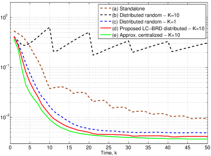
Figure 8: Sum of traces of error covariance matrices for all targets during time in the setting with $T=5$ targets, $N=3$ radars, $m=2$ measurements per scan and update time $t_{u}=0.25\,s$.

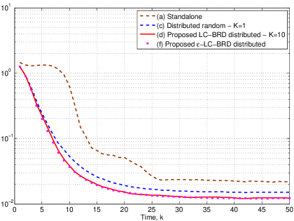
Figure 9: A setting with $T=15$ targets, $N=3$ radars, $m=6$ measurements per scan and update time $t_{u}=0.25\,s$.

Figure 8 compares the above strategies. The results are averaged over 100 realizations. Not surprisingly, due to the high process’ dynamics, a standalone, non-cooperative radar experiences weak performance since it utilizes only its own measurements which are not sufficient to cover all targets. Although approach in (b) uses $N\cdot m=6$ measurements, due to the lack of coordination it performs poorly. However, the distributed random strategy can be significantly improved if strategies are constantly being changed, given that there are no track migration costs involved. Note that the proposed LC-BRD distributed algorithm, which learns underlying NE allocations, outperforms the aforementioned strategies. On the other hand, it closely approaches the performance of the approximated centralized one while mitigating its inherent complexity.

The results related to a setting with more targets and measurements per scan than in the previous setting are plotted in Fig. 9. Here, we also include:

• $\epsilon$-LC-BRD distributed – The proposed low-complexity BRD-based distributed algorithm seeking NE and where each radar may change its strategy (even if in an NE) with a small $\epsilon$ probability. The probabilities $\alpha$ and $\epsilon$ are chosen to be $0.5$ and $0.02$, respectively.

Although without the curve for approximated centralized solution as a benchmark, the results that Figure 9 provides are similar to those in Fig. 8. Also, note that the two versions of the proposed LC-BRD algorithm exhibit pretty similar performance.

For the plots in Figs. 10-11, two additional radars in the network are considered w.r.t. the setting in Fig. 7, i.e., $(x_{4},y_{4})=[-4\,km$, $0\,km]$, $(x_{5},y_{5})=[7\,km$, $0\,km]$. This is probably the least favorable scenario for LC-BRD w.r.t. the distributed totally random ($K=1$) algorithm due to the fact that now $mod(N\cdot m,\,T)=0$, i.e., all targets can be selected with the same number of measurements. In Figs. 10-11, the update time is set to $t_{u}=0.25\,s$ and $t_{u}=0.025\,s$, respectively. Also, in Fig. 11 the following strategy is used in the comparison:

• RM distributed – The proposed distributed algorithm based on Regret-Matching which tracks CE, with $\theta_{k}=0.5$.

It can be noticed that the RM distributed algorithm clearly outperforms other distributed strategies. This is due to its more sophisticated learning mechanism, which comes at the expense of somewhat higher computational complexity than the other distributed strategies.

Figure 10: A setting with $T=5$ targets, $N=5$ radars, $m=2$ and update time $t_{u}=0.25\,s$.

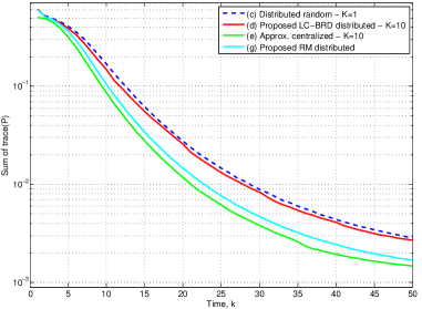
Figure 11: Scenario is same as in Fig. 10 except that $t_{u}=0.025\,s$ and the comparison is made with the proposed distributed algorithm based on Regret-Matching.

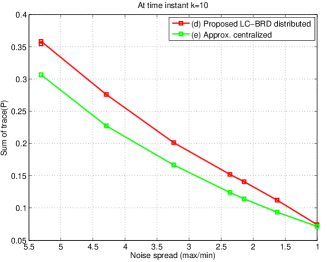
Figure 12: Performance comparison as a function of the measurements diversity in terms of the noise variance spread, for the same setting as in Fig. 11.

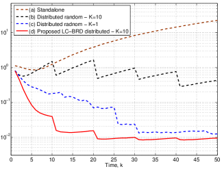
Figure 13: Scenario with $3\leq|\mathcal{T}_{i}|\leq 5$, $5\leq|\mathcal{N}_{i}|\leq 6$ and $W=\mathrm{1}_{N}\cdot\mathrm{1}^{T}_{|\mathcal{T}|}$, where it holds $\bigcup_{i\in\mathcal{N}_{i}}\mathcal{T}_{i}=\mathcal{T}$, $\forall i\in\mathcal{N}$.

Regarding the LC-BRD algorithm, it should be mentioned that its performance difference w.r.t. the centralized approach mainly depends on the measurement diversity, as suggested by Props.1-2 in Sec. IV. Specifically, the more similar measurements’ quality is, the gap w.r.t. the centralized approach is smaller ($PoA\rightarrow 1)$. This is illustrated in Fig. 12 by simulating the performance of the LC-BRD and the approximated centralized solution as a function of the noise variance spread in the network over all targets, i.e., $\textrm{max}_{i,j}(\sigma^{(i)}_{r_{j}})/\textrm{min}_{i,j}(\sigma^{(i)}_{r_{j}})$.

So far, the focus has been on the scenarios where all radars had the same interests, full observability and the radar network was fully connected. Now, let us remove these restrictions by firstly analyzing the scenario where the observability of each radar varies between $3$ and $5$ and the radar connectivity for some radars is not full while all radars are still interested in all targets. We set $T=5$ targets, $N=6$ radars, $m=1$ measurements per scan and update time $t_{u}=0.25\,s$. Note that the compared algorithms were modified accordingly in order to take into account the above constraints. As it can be seen in Fig. 13, the LC-BRD algorithm clearly outperforms the distributed random one ($K=1$) due to the fact that the equally balanced target allocations (from a single radar perspective) are not necessary reasonable, in contrast to the scenario in Figs. 10-11.

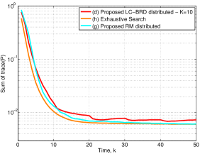
(a) Interest: All targets

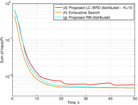
(b) Interest: 4 targets

Figure 14: Scenario with $|\mathcal{T}_{i}|=4$ and $\mathcal{N}_{i}=\mathcal{N}$, with $T=5$, $N=6$, $m=1$ and $t_{u}=0.25\,s$. The case where all radars have the same interests (all targets) is in 14(a), and the case where their interests differ in general is in 14(b).

Finally, we compare the proposed strategies with the centralized solution based on exhaustive search, i.e.,

• Exhaustive Search - The centralized search is implemented with full knowledge of all radars’ interests, observability and connectivity conditions and at each time instant the best allocation optimizing the sum of all radars’ utilities is selected.

Figure 14 shows that the LC-BRD performs well given its complexity. Note also that for the case where the interests of the radars are not necessary the same four targets, there are no theoretical guarantees that the NE exist(s) nor that a BRD-based algorithm may achieve an NE point; however, the LC-BRD still preforms relatively well. On the other hand, the RM-based algorithm, which is designed for more general scenarios, performs better than the LC-BRD and it closely approaches the centralized, exhaustive search solution.

VII Conclusions

In this article, we have proposed a new formulation of the track selection problem for a multi-target tracking scenario in an MFR network using the non-cooperative games. The target selections of each radar are considered to be autonomous; there is no central entity to tell radars what to do nor is there any negotiation process among the radars. We have analyzed two indicative scenarios with equal and heterogeneous conditions of observability and connectivity as well as radar interests. In the former scenario, the Nash equilibria of the underlying anti-coordination games have been analyzed and a simple yet effective distributed algorithm that introduces a balancing effect in track selections has been proposed. Afterwards, for a more demanding scenario, the solution concept of correlated equilibria has been employed and a more sophisticated, distributed algorithm based on the regret-matching has been proposed. Finally, computer simulations have verified that both proposed algorithms closely approximate the centralized solution while mitigating its inherent complexity.

References

- [1] A. O. Hero and D. Cochran, “Sensor management: Past, present, and future,” Sensors Journal, IEEE, vol. 11, no. 12, pp. 3064–3075, 2011.
- [2] S. Sabatini and M. Tarantino, Multifunction array radar. Artech House, 1994.
- [3] M. A. Richards, J. Scheer, and W. A. Holm, Principles of modern radar. SciTech Publishing, 2010.
- [4] S. S. Blackman and R. Popoli, Design and Analysis of Modern Tracking Systems, ser. Artech House radar library. Artech House, 1999.
- [5] Y. Bar-Shalom, “Multitarget-multisensor tracking: advanced applications,” Norwood, MA, Artech House, 1990, 391 p., vol. 1, 1990.
- [6] M. Mallick, V. Krishnamurthy, and B.-N. Vo, Integrated tracking, classification, and sensor management: theory and applications. John Wiley & Sons, 2012.
- [7] R. P. S. Mahler, Statistical Multisource-Multitarget Information Fusion. Norwood, MA, USA: Artech House, Inc., 2007.
- [8] S. P. Sira, Y. Li, A. Papandreou-Suppappola, D. Morrell, D. Cochran, and M. Rangaswamy, “Waveform-agile sensing for tracking,” IEEE Signal Processing Magazine, vol. 26, no. 1, pp. 53–64, Jan 2009.
- [9] Z. Ding, “A survey of radar resource management algorithms,” in Proc. Canadian Conference on Electrical and Computer Engineering, May 2008, pp. 001 559–001 564.
- [10] F. Katsilieris, “Sensor management for surveillance and tracking: An operational perspective,” Ph.D. dissertation, TU Delft, Delft University of Technology, 2015.
- [11] A. Charlish, “Autonomous agents for multi-function radar resource management,” Ph.D. dissertation, UCL (University College London), 2011.
- [12] F. Katsilieris, H. Driessen, and A. Yarovoy, “Threat-based sensor management for target tracking,” IEEE Transactions on Aerospace and Electronic Systems, vol. 51, no. 4, pp. 2772–2785, Oct 2015.
- [13] A. S. Narykov, O. A. Krasnov, and A. Yarovoy, “Algorithm for resource management of multiple phased array radars for target tracking,” in Proc. 16th Int. Conference on Information Fusion (FUSION 2013). IEEE, 2013, pp. 1258–1264.
- [14] G. van Keuk and S. S. Blackman, “On phased-array radar tracking and parameter control,” IEEE Transactions on Aerospace Electronic Systems, vol. 29, pp. 186–194, 1993.
- [15] W. Koch, “On adaptive parameter control for phased-array tracking,” in Signal and Data Processing of Small Targets, 1999, pp. 444–455.
- [16] S. Coetzee, K. Woodbridge, and C. Baker, “Multifunction radar resource management using tracking optimisation,” DTIC Document, Tech. Rep., 2005.
- [17] J. H. Zwaga and H. Driessen, “Tracking performance constrained MFR parameter control: applying constraints on prediction accuracy,” in Proc. 8th International Conference on Information Fusion, 2005, vol. 1, July 2005, pp. 546–551.
- [18] J. Hansen, R. Rajkumar, J. Lehoczky, and S. Ghosh, “Resource management for radar tracking,” in IEEE Conference on Radar, 2006. IEEE, 2006, p. 8.
- [19] V. Krishnamurthy and D. V. Djonin, “Optimal threshold policies for multivariate POMDPs in radar resource management,” IEEE Transactions on Signal Processing, vol. 57, no. 10, pp. 3954–3969, Oct 2009.
- [20] M. Kalandros, “Covariance control for multisensor systems,” IEEE Transactions on Aerospace and Electronic Systems, vol. 38, no. 4, pp. 1138–1157, Oct 2002.
- [21] H. Sherwani and H. D. Griffiths, “Tracking parameter control in multifunction radar network incorporating information sharing,” in 2016 19th International Conference on Information Fusion (FUSION), July 2016, pp. 319–326.
- [22] T. A. Severson and D. A. Paley, “Optimal sensor coordination for multitarget search and track assignment,” IEEE Transactions on Aerospace and Electronic Systems, vol. 50, no. 3, pp. 2313–2320, July 2014.
- [23] Y. Fu, Q. Ling, and Z. Tian, “Distributed sensor allocation for multi-target tracking in wireless sensor networks,” IEEE Transactions on Aerospace and Electronic Systems, vol. 48, no. 4, pp. 3538–3553, October 2012.
- [24] Y. Shoham and K. Leyton-Brown, Multiagent Systems: Algorithmic, Game-Theoretic, and Logical Foundations. Cambridge University Press, 2008.
- [25] J. R. Marden, G. Arslan, and J. S. Shamma, “Cooperative control and potential games,” IEEE Transactions on Systems, Man, and Cybernetics, Part B (Cybernetics), vol. 39, no. 6, pp. 1393–1407, Dec 2009.
- [26] Z. Han, D. Niyato, W. Saad, T. Baar, and A. Hjørungnes, Game Theory in Wireless and Communication Networks: Theory, Models, and Applications, 1st ed. New York, NY, USA: Cambridge University Press, 2012.
- [27] G. Bacci, S. Lasaulce, W. Saad, and L. Sanguinetti, “Game theory for networks: A tutorial on game-theoretic tools for emerging signal processing applications,” IEEE Signal Processing Magazine, vol. 33, no. 1, pp. 94–119, Jan 2016.
- [28] C. U. Saraydar, N. B. Mandayam, and D. Goodman, “Efficient power control via pricing in wireless data networks,” IEEE Transactions on Communications, vol. 50, no. 2, pp. 291–303, Feb 2002.
- [29] E. G. Larsson and E. A. Jorswieck, “Competition versus cooperation on the MISO interference channel,” IEEE Journal on Selected Areas in Communications, vol. 26, no. 7, pp. 1059–1069, September 2008.
- [30] G. Scutari, D. P. Palomar, and S. Barbarossa, “Competitive design of multiuser mimo systems based on game theory: A unified view,” IEEE Journal on Selected Areas in Communications, vol. 26, no. 7, pp. 1089–1103, 2008.
- [31] M. Felegyhazi, M. Cagalj, and J.-P. Hubaux, “Efficient mac in cognitive radio systems: A game-theoretic approach,” IEEE Transactions on Wireless Communications, vol. 8, no. 4, pp. 1984–1995, April 2009.
- [32] N. Bogdanović, D. Ampeliotis, and K. Berberidis, “Coalitional game theoretic approach to distributed adaptive parameter estimation,” in Proc. 2015 IEEE Int. Conference on Acoustics, Speech and Signal Processing (ICASSP), April 2015.
- [33] S. Gogineni and A. Nehorai, “Game theoretic design for polarimetric MIMO radar target detection,” Signal Processing, vol. 92, no. 5, pp. 1281–1289, 2012.
- [34] K. Han and A. Nehorai, “Jointly optimal design for MIMO radar frequency-hopping waveforms using game theory,” IEEE Transactions on Aerospace and Electronic Systems, vol. 52, no. 2, pp. 809–820, 2016.
- [35] M. Piezzo, A. Aubry, S. Buzzi, A. De Maio, and A. Farina, “Non-cooperative code design in radar networks: a game-theoretic approach,” EURASIP Journal on Advances in Signal Processing, vol. 2013, no. 1, pp. 1–17, 2013.
- [36] X. Song, P. Willett, S. Zhou, and P. B. Luh, “The MIMO radar and jammer games,” IEEE Transactions on Signal Processing, vol. 60, no. 2, pp. 687–699, Feb 2012.
- [37] G. Bacci, L. Sanguinetti, M. Greco, and M. Luise, “A game-theoretic approach for energy-efficient detection in radar sensor networks,” in Proc. 7th Sensor Array and Multichannel Signal Processing Workshop (SAM), June 2012, pp. 157–160.
- [38] H. Chen, S. Ta, and B. Sun, “Cooperative game approach to power allocation for target tracking in distributed MIMO radar sensor networks,” IEEE Sensors Journal, vol. PP, no. 99, pp. 1–1, 2015.
- [39] P. Chavali and A. Nehorai, “Concurrent particle filtering and data association using game theory for tracking multiple maneuvering targets,” IEEE Transactions on Signal Processing, vol. 61, no. 20, pp. 4934–4948, 2013.
- [40] A. Charlish, K. Woodbridge, and H. Griffiths, “Multi-target tracking control using continuous double auction parameter selection,” in Proc. 15th International Conference on Information Fusion (FUSION 2012). IEEE, 2012, pp. 1269–1276.
- [41] ——, “Phased array radar resource management using continuous double auction,” IEEE Transactions on Aerospace and Electronic Systems, vol. 51, no. 3, pp. 2212–2224, July 2015.
- [42] N. Bogdanović, H. Driessen, and A. Yarovoy, “Track selection in multifunction radars for multi-target tracking: An anti-coordination game,” in 2016 IEEE International Conference on Acoustics, Speech and Signal Processing (ICASSP), March 2016, pp. 3131–3135.
- [43] R. J. Aumann, “Subjectivity and correlation in randomized strategies,” Journal of Mathematical Economics, vol. 1, no. 1, pp. 67 – 96, 1974.
- [44] S. Hart and A. Mas-Colell, Simple adaptive strategies: from regret-matching to uncoupled dynamics. World Scientific, 2013, vol. 4.
- [45] N. Nisan, T. Roughgarden, E. Tardos, and V. V. Vazirani, Algorithmic Game Theory. Cambridge University Press, 2007.
- [46] Y. Bramoullé, “Anti-coordination and social interactions,” Games and Economic Behavior, vol. 58, no. 1, pp. 30–49, 2007.
- [47] E. Rasmusen, Games and information. Blackwell Publishers, 2001.
- [48] C. H. Papadimitriou, Computational complexity. John Wiley and Sons Ltd., 2003.
- [49] N. Bogdanović, J. Plata-Chaves, and K. Berberidis, “Distributed incremental-based LMS for node-specific adaptive parameter estimation,” IEEE Transactions on Signal Processing, vol. 62, no. 20, pp. 5382–5397, Oct 2014.
- [50] D. Monderer and L. S. Shapley, “Potential games,” Games and Economic Behavior, vol. 14, no. 1, pp. 124 – 143, 1996.
- [51] S. Hart and A. Mas-Colell, “A simple adaptive procedure leading to correlated equilibrium,” Econometrica, vol. 68, no. 5, pp. 1127–1150, 2000.
- [52] M. Maskery, V. Krishnamurthy, and Q. Zhao, “Decentralized dynamic spectrum access for cognitive radios: cooperative design of a non-cooperative game,” IEEE Transactions on Communications, vol. 57, no. 2, pp. 459–469, February 2009.
- [53] H. Kushner and G. G. Yin, Stochastic approximation and recursive algorithms and applications. Springer Science & Business Media, 2003, vol. 35.