Encoding Cardinality Constraints using Generalized Selection Networks

Abstract

Boolean cardinality constraints state that at most (at least, or exactly) $k$ out of $n$ propositional literals can be true. We propose a new class of selection networks that can be used for an efficient encoding of them. Several comparator networks have been proposed recently for encoding cardinality constraints and experiments have proved their efficiency. Those were based mainly on the odd-even or pairwise comparator networks. We use similar ideas, but we extend the model of comparator networks so that the basic components are not only comparators (2-sorters) but more general $m$-sorters, for $m\geq 2$. The inputs are organized into $m$ columns, in which elements are recursively selected and, after that, columns are merged using an idea of multi-way merging. We present two algorithms parametrized by $m\geq 2$. We call those networks $m$-Wise Selection Network and $m$-Odd-Even Selection Network. We give detailed construction of the mergers when $m=4$. The construction can be directly applied to any values of $k$ and $n$. The proposed encoding of sorters is standard, therefore the arc-consistency is preserved. We prove correctness of the constructions and present the theoretical and experimental evaluation, which show that the new encodings are competitive to the other state-of-art encodings.

1 Introduction

Several hard decision problems can be efficiently reduced to Boolean satisfiability (SAT) problem and tried to be solved by recently-developed SAT-solvers. Some of them are formulated with the help of different high-level constraints, which should be either encoded into CNF formulas or solved inside a SAT-solver by a specialized extension. There was much research on both of these approaches.

In this paper we consider encodings of Boolean cardinality constraints that take the form $x_{1}+x_{2}+\dots+x_{n}\sim k$, where $x_{1},x_{2},\dots,x_{n}$ are Boolean literals (that is, variables or their negations) and $\sim$ is a relation from the set $\{<,\leq,=,\geq,>\}$. Such cardinality constraints appear naturally in formulations of different real-world problems including cumulative scheduling [16], timetabling [4] or formal hardware verification [8].

In a direct encoding of a cardinality constraint $x_{1}+x_{2}+\dots+x_{n}<k$ one can take all subsets of $X=\{x_{1},\dots,x_{n}\}$ of size $k$ and for each of them construct a CNF formula that states that at least one of the literals in the subset must be false. The direct encoding is quite efficient for very small values of $k$ and $n$, but for larger parameters another approach should be used.

Related work: In the last years several selection networks were proposed for the encoding cardinality constraints and experiments proved their efficiency. They were based mainly on the odd-even or pairwise comparator networks. Codish and Zazon-Ivry [9] introduced pairwise selection networks that used the concept of Parberry’s pairwise sorting network [15]. Abío, Nieuwenhuis, Oliveras and Rodríguez-Carbonell [1, 3] defined encodings that implemented the odd-even sorting networks by Batcher [6]. In [1] the authors proposed a mixed parametric approach to the encodings, where the direct encoding is chosen for small sub-problems and the splitting point is optimized when large problems are divided into two smaller ones. They proposed to minimize the function $\lambda\cdot num\_vars+mun\_clauses$ in the encodings. The constructed encodings are small and efficient, but non-trivial extra time is needed to find the optimal splitting points.

Our contribution: Partially inspired by this optimization criterion we started looking for selection networks that can be encoded with a smaller number of auxiliary variables and, if possible, not much larger number of clauses, and where there is no need for the costly optimization. In addition, we investigate the influence of our encodings on the execution times of SAT-solvers to be sure that the new algorithms can be used in practice. The obtained constructions are presented in this paper. The main idea is to split the problem into $m$ sub-problems, recursively select elements in them and then merge the selected subsequences using an idea of multi-way merging [7, 11]. In such approach we can use not only comparators (2-sorters) but also $m$-sorters, which can be encoded directly.

Using this generalized version of comparators we have created two novel classes of networks parametrized by $m\geq 2$. First one is called $m$-Wise Selection Network, in which we use the idea of pairwise sorting [15] combined with a multi-way merging algorithm by Gao, Liu and Zhao [11], but in more general way. The second class is called $m$-Odd-Even Selection Networks, where the multi-way merge sorting networks by Batcher and Lee [7] are generalized in a way that we can recursively select $k$ largest elements from each of the $m$ sub-problems. It should be also pointed out that none of the algorithms presented in this paper is using or is even based on the construction presented in the CP’15 paper of Karpiński and Piotrów [12]. The reason is that there the size of an input sequence is required to be a power of 2.

Both algorithms are presented using divide and conquer paradigm. The key to achieve efficient algorithms lie in the construction of networks that combines the results obtained from the recursive calls. The construction of those mergers is the main result of this paper. We fix $m=4$ and give detailed constructions for two merging networks: $4$-Wise Merging Network and $4$-Odd-Even Merging Network. We prove their correctness and compare the numbers of variables and clauses of the corresponding encodings to their two counterparts: Pairwise Merging Networks and Odd-Even Merging Networks [9]. The calculations show that encodings based on our merging networks uses less number of variables and clauses, when $k<n$. In case of $4$-Odd-Even Merging Network this also translates into smaller encodings in terms of variables and clauses for the $4$-Odd-Even Selection Network in comparison to Odd-Even Selection Network, for sufficiently large $k$ and $n$.

The constructions are parametrized by any values of $k$ and $n$, so they can be further optimized by mixing them with other constructions. For example, in our experiments we mixed them with the direct encoding for small values of parameters. We used the standard encoding of $m$-sorters, therefore the arc consistency is preserved. Finally, we present results of our experiments, which is another main contribution of this paper. We show that generalized selection networks are superior to standard selection networks previously proposed in the literature, in context of translating cardinality constraints into propositional formulas. We also conclude that although encodings based on pairwise approach use less number of variables than odd-even encodings, in practice, it is the latter that achieve better reduction in SAT-solving runtime. It is a helpful observation, because from the practical point of view, implementing odd-even networks is a little bit easier.

We also empirically compare our encodings with other state-of-art encodings, not only based on comparator networks, but also on binary adders and binary decision diagrams. Those are mainly used in encodings of Pseudo-Boolean constraints, but it is informative to see how well they perform when encoding cardinality constraints.

Structure of the paper: The rest of the paper is organized as follows: Section 2 contains definitions and notations used in the paper. In Section 3 the construction of the generalized selection networks and the proofs of correctness are given. Section 4 is devoted to specialized merging networks for $m=4$ and contains detailed proofs of correctness. In Section 5 we compare the encodings produced by the construction with Pairwise Cardinality Network and Odd-Even Selection Network, in terms of number of variables and clauses each of them uses. Our experimental evaluation is presented in Section 6 followed by Conclusions.

2 Preliminaries

In this section we introduce definitions and notations used in the rest of the paper. Let $X$ denote a totally ordered set, for example the set of natural numbers $\mathbb{N}$ or the set of binary values $\{0,1\}$. We introduce the auxiliary ”smallest” element $\bot\notin X$, such that for all $x\in X$ we have $\bot<x$. Thus, $X\cup\{\bot\}$ is totally ordered. The element $\bot$ is used in the next section to simplify presentation of algorithms.

Definition 1 (sequences).

A sequence of length $n$, say $\bar{x}=\langle x_{1},\dots,x_{n}\rangle$, is an element of $X^{n}$. In particular, an element of $\{0,1\}^{n}$ is called a binary sequence. We say that a sequence $\bar{x}\in X^{n}$ is sorted if $x_{i}\geq x_{i+1}$, $1\leq i<n$. Given two sequences $\bar{x}=\langle x_{1},\dots,x_{n}\rangle$ and $\bar{y}=\langle y_{1},\dots,y_{m}\rangle$ we define concatenation as $\bar{x}::\bar{y}=\langle x_{1},\dots,x_{n},y_{1},\dots,y_{m}\rangle$. We use also the following subsequence notation: $\bar{x}_{\textit{odd}}=\langle x_{1},x_{3},\dots\rangle$, $\bar{x}_{\textit{even}}=\langle x_{2},x_{4},\dots\rangle$, $\bar{x}_{a,\dots,b}=\langle x_{a},\dots,x_{b}\rangle$, $1\leq a\leq b\leq n$, and the prefix/suffix operators: $pref(i,\bar{x})~{}=~{}\bar{x}_{1,\dots,i}$ and $suff(i,\bar{x})~{}=~{}\bar{x}_{i,\dots,n}$, $1\leq i\leq n$. The number of a given value $b$ in $\bar{x}$ is denoted by $|\bar{x}|_{b}$ and the result of removing all occurrences of $b$ in $\bar{x}$ is written as $\textrm{drop}(b,\bar{x})$.

Let $n,m\in\mathbb{N}$. We define a domination relation ’$\succeq$’ on $X^{n}\times X^{m}$. Let $\bar{x}\in X^{n}$ and $\bar{y}\in X^{m}$, then: $\bar{x}\succeq\bar{y}\iff\forall_{i\in\{1,\dots,n\}}\forall_{j\in\{1,\dots,m\}}\;x_{i}\geq y_{j}$

Definition 2 (zip operator).

For $m\geq 1$ given sequences (column vectors) $\bar{x}^{i}=\langle x^{i}_{1},x^{i}_{2},\dots,x^{i}_{n_{i}}\rangle$, $1\leq i\leq m$ and $n_{1}\geq n_{2}\geq\dots\geq n_{m}$, let us define the zip operation that outputs the elements of the vectors in row-major order:

$$\textrm{zip}(\bar{x}^{1},\dots,\bar{x}^{m})=\begin{cases}\bar{x}^{1}&\mbox{if~{}}m=1\\ \textrm{zip}(\bar{x}^{1},\dots,\bar{x}^{m-1})&\mbox{if~{}}|\bar{x}^{m}|=0\\ \langle x^{1}_{1},x^{2}_{1},\dots,x^{m}_{1}\rangle::\textrm{zip}(\bar{x}^{1}_{2,\dots,n_{1}},\dots,\bar{x}^{m}_{2,\dots,n_{m}})&\mbox{otherwise}\end{cases}$$

We construct and use comparator networks in this paper. The standard definitions and properties of them can be found, for example, in [13]. The only difference is that we assume that the output of any sorting operation or comparator is in a non-increasing order.

Definition 3 (m-sorter).

A comparator network $f^{m}$ is a sorting network (or m-sorter), if for each $\bar{x}\in X^{m}$, $f^{m}(\bar{x})$ is sorted.

In the pairwise sorting network, the first step is to split the input into two equally sized sequences $\bar{x}$ and $\bar{y}$, such that for any $i$, $x_{i}\geq y_{i}$. Then $\bar{x}$ and $\bar{y}$ are sorted independently and finally merged. Even after sorting, the property $x_{i}\geq y_{i}$ is maintained (see [15]). For example, the pair of sequences $\langle 110,100\rangle$ are pairwise sorted. We would like to extend this notion to cover larger number of sequences, let’s say $m\geq 2$. For example, the tuple $\langle 111,110,100,000\rangle$ is 4-wise (sorted). The following definition captures this idea.

Definition 4 (m-wise sequences).

Let $c,k,m\in\mathbb{N}$, $1\leq k$ and $k/m\leq c$. Moreover, let $k_{i}=\min(c,\left\lfloor k/i\right\rfloor)$ and $\bar{x}^{i}\in X^{k_{i}}$, $1\leq i\leq m$. The tuple $\langle\bar{x}^{1},\dots,\bar{x}^{m}\rangle$ is $m$-wise of order $(c,k)$ if:

1. $\forall_{1\leq i\leq m}$ $\bar{x}^{i}$ is sorted,

2. $\forall_{1\leq i\leq m-1}$ $\forall_{1\leq j\leq n_{i+1}}$ $x^{i}_{j}\geq x^{i+1}_{j}$.

Observation 1.

Let a tuple $\langle\bar{x}^{1},\dots,\bar{x}^{m}\rangle$ be $m$-wise of order $(c,k)$. Then:

1. $|\bar{x}^{1}|\geq|\bar{x}^{2}|\geq\dots\geq|\bar{x}^{m}|=\left\lfloor k/m\right\rfloor$,

2. $\sum_{i=1}^{m}|\bar{x}^{i}|\geq k$,

3. if $|\bar{x}^{i-1}|>|\bar{x}^{i}|+1$ then $|\bar{x}^{i}|=\left\lfloor k/i\right\rfloor$.

Proof.

The first statement is obvious. To prove the second one let $k_{i}=|\bar{x}^{i}|$, $1\leq i\leq m$. Then, if $k_{i}=c$ for each $1\leq i\leq m$, we have $\sum_{i=1}^{m}k_{i}=mc\geq mk/m=k$ and we are done. Let $1\leq i\leq m$ be the first index such that $k_{i}\neq c$, therefore $k_{i}=\left\lfloor k/i\right\rfloor<c$. Thus, for each $1\leq j<i$: $k_{j}=c>k_{i}$, therefore $k_{j}\geq k_{i}+1$. From this we get that $\sum_{j=1}^{m}k_{j}\geq\sum_{j=1}^{i}k_{j}\geq i\left\lfloor k/i\right\rfloor+i-1\geq k$.

The third one can be easily proved by contradiction. Assume that $k_{i}=c$, then from the first property $k_{i-1}\geq k_{i}=c$. Therefore, $k_{i-1}=\min(c,\left\lfloor k/(i-1)\right\rfloor)\geq c$, so $k_{i-1}=c$, a contradiction. ∎

Definition 5 (top $k$ sorted sequence).

A sequence $\bar{x}\in X^{n}$ is top $k$ sorted, with $k\leq n$, if $\langle x_{1},\dots,x_{k}\rangle$ is sorted and $\langle x_{1},\dots,x_{k}\rangle\succeq\langle x_{k+1},\dots,x_{n}\rangle$.

Definition 6 (m-wise merger).

A comparator network $f^{s}_{(c,k)}$ is a m-wise merger of order $(c,k)$, if for each $m$-wise tuple $T=\langle\bar{x}^{1},\dots,\bar{x}^{m}\rangle$ of order $(c,k)$, such that $s=\sum_{i=1}^{m}|\bar{x}^{i}|$, $f^{s}_{(c,k)}(T)$ is top $k$ sorted.

Definition 7 (m-odd-even merger).

A comparator network $f^{s}_{k}$ is a m-odd-even merger of order $k$, if for each tuple $T=\langle\bar{x}^{1},\dots,\bar{x}^{m}\rangle$, where each $\bar{x}^{i}$ is top $k$ sorted and $s=\sum_{i=1}^{m}|\bar{x}^{i}|$, $f^{s}_{k}(T)$ is top $k$ sorted.

Definition 8 (selection network).

A comparator network $f^{n}_{k}$ (where $k\leq n$) is a $k$-selection network, if for each $\bar{x}\in X^{n}$, $f^{n}_{k}(\bar{x})$ is top $k$ sorted.

A clause is a disjunction of literals (Boolean variables $x$ or their negation $\neg x$). A CNF formula is a conjunction of one or more clauses. Cardinality constraints are of the form $x_{1}+\dots+x_{n}\sim k$, where $k\in\mathbb{N}$ and $\sim$ belongs to $\{<,\leq,=,\geq,>\}$. We will focus on cardinality constraints with less-than relation, i.e. $x_{1}+\dots+x_{n}<k$. The other can be easily translated to such form (see [3]).

In [1, 3, 9, 10] authors are using sorting networks for an encoding of cardinality constraints, where inputs and outputs of a comparator are Boolean variables and comparators are encoded as a CNF formula. In addition, the $k$-th greatest output variable $y_{k}$ of the network is forced to be 0 by adding $\neg y_{k}$ as a clause to the formula that encodes $x_{1}+\dots+x_{n}<k$. We use similar approach, but rather than using simple comparators (2-sorters), we also use comparators of higher order as building blocks. The $m$-sorter can be encoded as follows: for input variables $\bar{x}$ and output variables $\bar{y}$, we add the set of clauses $\{x_{i_{1}}\wedge\dots\wedge x_{i_{p}}\Rightarrow y_{p}\,:\,1\leq p\leq m,1\leq i_{1}<\dots<i_{p}\leq m\}$. Therefore, we need $m$ auxiliary variables and $2^{m}-1$ clauses.

3 Generalized Selection Networks

Here we present two novel constructions for selection networks which uses sorters of arbitrary size as components. We want to apply our algorithms for CNF encoding, therefore the only non-trivial operation that we are allowed to use in generalized comparator networks is $sort^{m}:X^{m}\rightarrow X^{m}$, which is a $m$-sorter. Here (and in the rest of the paper) we use it as a black box, but keep in mind that in the actual implementation one should encode the $m$-sorter using the standard procedure explained at the end of Section 2. We would also like to note that only first $k$ output variables for each selection network is of interest, but to stay consistent with the definitions of Section 2, we write our algorithms so that the size of the output is the same as the size of the input. To this end we introduce the variable $\overline{out}$ in which we store all throw-away variables in arbitrary order. The sequence $\overline{out}$ is then appended to the output of the algorithms.

3.1 m-Wise Selection Network

We begin with the algorithm for constructing the $m$-Wise Selection Network (Network 1) and we prove that it is correct. In Network 1 we use $mw\_merge^{s}_{(c,k)}$, that is, a $m$-Wise Merger of order $(c,k)$, as a block box. We give detailed constructions of $m$-Wise Merger for $m=4$ in the next section.

The idea we use is the generalization of the one used in Pairwise Cardinality Network from [9] which is based on the Pairwise Sorting Network by Parberry [15]. First, we split the input sequence into $m$ columns of non-increasing sizes (lines 2–5) and we sort rows using sorters (lines 6–8). Then we recursively run the selection algorithm on each column (lines 9–11), where at most $\left\lfloor k/i\right\rfloor$ items are selected from the $i$-th column. In obtained outputs, selected items are sorted and form prefixes of the columns. The prefixes are padded with zeroes (with $\bot$’s) in order to get the input sizes required by the $m$-wise property (Definition 4) and, finally, they are passed to the merging procedure (line 12–13). The base case, when $k=1$, is handled by the auxiliary network $max^{n}$, which outputs the maximum of $n$ elements. The standard construction of $max^{n}$ uses $n-1$ 2-sorters.

Example 1.

In Figure 1 we present a sample run of Network 1. The input is a sequence $1111010010000010000101$, with parameters $\langle n_{1},n_{2},n_{3},n_{4},k\rangle=\langle 8,7,4,3,6\rangle$. First step (Figure 1a) is to arrange the input in columns (lines 2–5). In this example we get $\bar{x}^{1}=\langle 11110100\rangle$, $\bar{x}^{2}=\langle 1000001\rangle$, $\bar{x}^{3}=\langle 0000\rangle$ and $\bar{x}^{4}=\langle 101\rangle$. Next we sort rows using $1,2,3$ or $4$-sorters (lines 6–8), the result is visible in Figure 1b. We make recursive calls in lines 9–11 of the algorithm. Items selected recursively in this step are marked on Figure 1c. Notice that in $i$-th column we only need to select $\left\lfloor k/i\right\rfloor$ largest elements. This is because of the initial sorting of the rows. Next comes the merging step, which is selecting $k$ largest elements from the results of the previous step. How exactly those elements are obtained and outputted depends on the implementation. We choose the convention that the resulting $k$ elements must be placed in the major-row order in our column representation of the input (see Figure 1d).

(a) split into columns

(b) sort rows

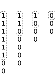
(c) select recursively

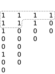
(d) merge columns

Figure 1: Sample run of the 4-Wise Slection Network.

Network 1 $mw\_sel^{n}_{k}$

1:$\bar{x}\in X^{n}$; $n_{1},\dots,n_{m}\in\mathbb{N}$ where $n>n_{1}\geq\dots\geq n_{m}$ and $\sum n_{i}=n$; $1\leq k\leq n$

2:if $k=1$ then return $max^{n}(\bar{x})$

3:$offset=1$

4:for all $i\in\{1,\dots,m\}$ do $\triangleright$ Splitting the input into columns.

5:     $\bar{x}^{i}\leftarrow\langle x_{offset},\dots,x_{offset+n_{i}-1}\rangle$

6:     $offset+=n_{i}$

7:for all $i\in\{1,\dots,n_{1}\}$ do $\triangleright$ Sorting rows.

8:     $m^{\prime}=\max\{j:n_{j}\geq i\}$

9:     $\bar{y}^{i}\leftarrow\textit{sort}^{m^{\prime}}(\langle x^{1}_{i},\dots,x^{m^{\prime}}_{i}\rangle)$

10:for all $i\in\{1,\dots,m\}$ do $\triangleright$ Recursively selecting items in columns.

11:     $k_{i}=\min(n_{1},\left\lfloor k/i\right\rfloor)$;   $l_{i}=\min(n_{i},\left\lfloor k/i\right\rfloor)$ $\triangleright$ $k_{i}\geq l_{i}$

12:     $\bar{z}^{i}\leftarrow mw\_sel^{n_{i}}_{l_{i}}(\bar{y}^{1}_{i},\dots,\bar{y}^{n_{i}}_{i})$

13:$s=\sum_{i=1}^{m}k_{i}$;   $c=k_{1}$;   $\overline{out}=\textrm{suff}(l_{1}+1,\bar{z}^{1})::\dots::\textrm{suff}(l_{m}+1,\bar{z}^{m})$

14:$\overline{res}\leftarrow mw\_merge^{s}_{(c,k)}(\langle pref(l_{1},\bar{z}^{1})::\bot^{k_{1}-l_{1}},\dots,pref(l_{m},\bar{z}^{m})\rangle::\bot^{k_{m}-l_{m}})$

15:return $\textrm{drop}(\bot,\overline{res})::\overline{out}$

In the following we will prove the correctness of Network 1 using the well-known 0-1 Principle, that is, we will consider binary sequences only.

Lemma 1.

Let $\bar{t}^{i}=\langle\bar{y}^{1}_{i},\dots,\bar{y}^{n_{i}}_{i}\rangle$, where $\bar{y}^{j}$, $j=1,\dots,n_{1}$, is the result of Step 8 in Network 1. For each $1\leq i<m$: $|\bar{t}^{i}|_{1}\geq|\bar{t}^{i+1}|_{1}$.

Proof.

Take any $1\leq i<m$. Consider element $y^{j}_{i}$ (for some $1\leq j\leq n_{i}$). Since $\bar{y}^{j}$ is sorted, we have $y^{j}_{i}\geq y^{j}_{i+1}$, therefore if $y^{j}_{i+1}=1$ then $y^{j}_{i}=1$. Thus $|\bar{t}^{i}|_{1}\geq|\bar{t}^{i+1}|_{1}$. ∎

Corollary 1.

For each $1\leq i\leq m$, let $\bar{z}^{i}$ be the result of the step 11 in Network 1. Then for each $1\leq i<m$: $|\bar{z}^{i}|_{1}\geq|\bar{z}^{i+1}|_{1}$.

Proof.

For $1\leq i\leq m$, let $\bar{t}^{i}$ be the same as in Lemma 1. Take any $1\leq i<m$. Comparator network only permutate its input, therefore $|\bar{z}^{i}|_{1}=|mw\_sel^{n_{i}}_{s_{i}}(\bar{t}^{i})|_{1}=|\bar{t}^{i}|_{1}\geq|\bar{t}^{i+1}|_{1}=|mw\_sel^{n_{i+1}}_{s_{i+1}}(\bar{t}^{i+1})|_{1}=|\bar{z}^{i+1}|_{1}$. The inequality comes from Lemma 1. ∎

Theorem 3.1.

$mw\_sel^{n}_{k}$ is a $k$-selection network.

Proof.

We prove by induction that for each $n,k\in\mathbb{N}$ such that $1\leq k\leq n$ and each $\bar{x}\in\{0,1\}^{n}$: $mw\_sel^{n}_{k}(\bar{x})$ is top $k$ sorted. If $1=k\leq n$ then $mw\_sel^{n}_{k}=max^{n}$, so the theorem is true. For the induction step assume that $n\geq k\geq 2$, $m\geq 2$ and for each $(n^{*},k^{*})\prec(n,k)$ (in lexicographical order) the theorem holds. We have to prove the following two properties:

1. The tuple $\langle pref(l_{1},\bar{z}^{1})::\bot^{k_{1}-l_{1}},\dots,pref(l_{m},\bar{z}^{m})::\bot^{k_{m}-l_{m}}\rangle$ is $m$-wise of order $(k_{1},k)$.

2. The sequence $\bar{w}=pref(l_{1},\bar{z}^{1})::\dots::pref(l_{m},\bar{z}^{m})$ contains $k$ largest elements from $\bar{x}$.

Ad. 1): Observe that for any $i$, $1\leq i\leq m$, we have $n_{i}\leq n_{1}<n$ and $l_{i}\leq l_{1}\leq k$. Thus, $(n_{i},l_{i})\prec(n,k)$ and $\bar{z}_{i}$ is top $l_{i}$ sorted due to the induction hypothesis. Therefore, $pref(l_{i},\bar{z}^{i})$ is sorted and so is $pref(l_{i},\bar{z}^{i})::\bot^{k_{i}-l_{i}}$. In this way, we prove that the first property of Definition 4 is satisfied. To prove the second one, fix $1\leq j\leq l_{i+1}$ and assume that $z^{i+1}_{j}=1$. We are going to show that $z^{i}_{j}=1$. Since $\bar{z}^{i}$ and $\bar{z}^{i+1}$ are both top $l_{i+1}$ sorted (by the induction hypothesis) and since $|\bar{z}^{i}|_{1}\geq|\bar{z}^{i+1}|_{1}$ (from Corollary 1), we have $|pref(l_{i+1},\bar{z}^{i})|_{1}\geq|pref(l_{i+1},\bar{z}^{i+1})|_{1}$, so $z^{i}_{j}=1$.

Ad. 2): It is easy to observe that $\bar{z}=\bar{z}^{1}::\dots::\bar{z}^{m}$ is a permutation of the input sequence $\bar{x}$. If all 1’s in $\bar{z}$ are in $\bar{w}$, we are done. So assume that there exists $z^{i}_{j}=1$ for some $1\leq i\leq m$, $l_{i}<j\leq n_{i}$. We will show that $|\bar{w}|_{1}\geq k$. From the induction hypothesis we get $pref(l_{i},z^{i})\succeq\langle z^{i}_{j}\rangle$, which implies that $|pref(l_{i},z^{i})|_{1}=l_{i}$. From (1) and the second property of Definition 4 it is clear that all $z^{s}_{t}$ are 1’s, where $1\leq s\leq i$ and $1\leq t\leq l_{i}$, therefore $|pref(l_{i},\bar{z}^{1})::\dots::pref(l_{i},\bar{z}^{i})|_{1}=i\cdot l_{i}$. Moreover, since $j>l_{i}$, we have $l_{i}=\left\lfloor k/i\right\rfloor$; otherwise we would have $j>n_{i}$. If $i=1$, then $|\bar{w}|_{1}\geq 1\cdot l_{1}=k$ and (2) holds.

Otherwise, $l_{1}>l_{i}$, so from the definition of $l_{i}$, $l_{1}\geq\dots\geq l_{i}$, hence there exists $r\geq 1$ such that $\forall_{r<i^{\prime}\leq i}$ $l_{r}>l_{i^{\prime}}=l_{i}$. Notice that since $|pref(l_{i},z^{i})|_{1}=l_{i}$ and $z^{i}_{j}=1$ where $j>l_{i}$ we get $|z^{i}|_{1}\geq l_{i}+1$. From Corollary 1 we have that for $1\leq r^{\prime}\leq r$: $|\bar{z}^{r^{\prime}}|_{1}\geq l_{i}+1$. Using $l_{r^{\prime}}\geq l_{r}>l_{i}$ and the induction hypothesis we get that each $\bar{z}^{r^{\prime}}$ is top $l_{i}+1$ sorted, therefore $|pref(l_{i}+1,\bar{z}^{r^{\prime}})|_{1}=l_{i}+1$. We finally have that $|\bar{w}|_{1}\geq|pref(l_{i}+1,\bar{z}^{1})::\dots::pref(l_{i}+1,\bar{z}^{r})::pref(l_{i},\bar{z}^{r+1})::\dots::pref(l_{i},\bar{z}^{i})|_{1}=r(l_{i}+1)+(i-r)l_{i}=r(l_{r+1}+1)+(i-r)l_{r+1}=i\cdot l_{r+1}+r\geq(r+1)\left\lfloor k/(r+1)\right\rfloor+r\geq k$. In the second to last inequality, we use the facts: $l_{r+1}=l_{i}=\left\lfloor k/i\right\rfloor<n_{i}\leq n_{r+1}$ from which $l_{r+1}=\left\lfloor k/(r+1)\right\rfloor$ follows.

From the statements (1) and (2) we can conclude that $mw\_merge^{s}_{(n,k)}$ will return the $k$ largest elements from $\bar{x}$, which completes the proof. ∎

3.2 m-Odd-Even Selection Network

Next we present the algorithm for constructing the $m$-Odd-Even Selection Network (Network 2) and we prove that it is correct. In Network 2 we use $oe\_merge^{s}_{k}$ as a black box. It is a $m$-Odd-Even Merger of order $k$. We give detailed constructions of $m$-Odd-Even Merger for $m=4$ in the next section.

The idea we use is the generalization of the one used in Odd-Even Selection Network from [9] which is based on the Odd-Even Sorting Network by Batcher [6]. We arrange the input sequence into $m$ columns of non-increasing sizes and we recursively run the selection algorithm on each column (lines 3–6), where at most $k$ items are selected from each column. Notice that each column is represented by ranges derived from the increasing value of variable $offset$. Selected items are sorted and form prefixes of the columns and they are the input to the merging procedure (line 7–8).

Example 2.

Assuming the same input sequence and parameters as in Example 1, the sample run of 4-Odd-Even Selection Network would be very similar to the one presented in Figure 1, except we would not do the row sorting step, and in consequence we would need to recursively select $k$ largest elements from each column.

Network 2 $oe\_sel^{n}_{k}$

1:$\bar{x}\in\{0,1\}^{n}$; $n_{1},\dots,n_{m}\in\mathbb{N}$ where $n>n_{1}\geq\dots\geq n_{m}$ and $\sum n_{i}=n$; $1\leq k\leq n$

2:if $k=1$ then return $max^{n}(\bar{x})$

3:$offset=1$

4:for all $i\in\{1,\dots,m\}$ do

5:     $k_{i}=\min(k,n_{i})$

6:     $\bar{y}^{i}\leftarrow oe\_sel^{n_{i}}_{k_{i}}(\langle x_{offset},\dots,x_{offset+n_{i}-1}\rangle)$

7:     $offset+=n_{i}$

8:$s=\sum_{i=1}^{m}k_{i}$;   $\overline{out}=\textrm{suff}(k_{1}+1,\bar{y}^{1})::\dots::\textrm{suff}(k_{m}+1,\bar{y}^{m})$

9:return $oe\_merge^{s}_{k}(\langle\textrm{pref}(k_{1},\bar{y}^{1}),\dots,\textrm{pref}(k_{m},\bar{y}^{m})\rangle)::\overline{out}$

Theorem 3.2.

$oe\_sel^{n}_{k}$ is a $k$-selection network.

Proof.

It is easy to observe that $\bar{y}=\bar{y}^{1}::\dots::\bar{y}^{m}$ is a permutation of the input sequence $\bar{x}$. We prove by induction that for each $n,k\in\mathbb{N}$ such that $1\leq k\leq n$ and each $\bar{x}\in\{0,1\}^{n}$: $oe\_sel^{n}_{k}(\bar{x})$ is top $k$ sorted. If $1=k\leq n$ then $oe\_sel^{n}_{k}=max^{n}$, so the theorem is true. For the induction step assume that $n\geq k\geq 2$, $m\geq 2$ and for each $(n^{*},k^{*})\prec(n,k)$ (in lexicographical order) the theorem holds. We have to prove that the sequence $\bar{w}=pref(k_{1},\bar{y}^{1})::\dots::pref(k_{m},\bar{y}^{m})$ contains $k$ largest elements from $\bar{x}$. If all 1’s in $\bar{y}$ are in $\bar{w}$, we are done. So assume that there exists $y^{i}_{j}=1$ for some $1\leq i\leq m$, $k_{i}<j\leq n_{i}$. We will show that $|\bar{w}|_{1}\geq k$. Notice that $k_{i}=k$, otherwise $j>k_{i}=n_{i}$ – a contradiction. Since $|\bar{y}^{i}|=n_{i}\leq n_{1}<n$, from the induction hypothesis we get that $\bar{y}^{i}$ is top $k_{i}$ sorted. In consequence, $pref(k_{i},\bar{y}^{i})\succeq\langle y^{i}_{j}\rangle$, which implies that $|pref(k_{i},y^{i})|_{1}=k_{i}=k$. We conclude that $|\bar{w}|_{1}\geq|pref(k_{i},y^{i})|_{1}=k$. Note also that in the case $n=k$ we have all $k_{i}=\min(n_{i},k)<k$, so the case is correctly reduced.

Finally, using $oe\_merge^{s}_{k}$ the algorithm returns $k$ largest elements from $\bar{x}$, which completes the proof. ∎

4 Merging Networks

In this section we give the detailed constructions of the networks $4mw\_merge$ and $4oe\_merge$ that merge four sequences (columns) obtained from the recursive calls in Networks 1 and 2. In the first construction we can assume that input columns form a tuple that is 4-wise, because rows were sorted before selecting top elements in each column. In the second one input columns are just top $k$ sorted and rows are sorted in the final steps of the merging process. In the subsections 4.1 and 4.2 we present the $4$-Wise Merger and $4$-Column Odd-Even Merger, respectively.

4.1 4-Wise Merging Networks

In this subsection the first merging algorithm for four columns is presented. The input to the merging procedure is $R=\langle pref(n_{1},\bar{y}^{1}),\dots,pref(n_{m},\bar{y}^{m})\rangle$, where each $\bar{y}^{i}$ is the output of the recursive call in Network 1. The main observation is the following: since $R$ is $m$-wise, if you take each sequence $pref(n_{i},\bar{y}^{i})$ and place them side by side, in columns, from left to right, then the sequences will be sorted in rows and columns. The goal of the networks is to put the $k$ largest elements in top rows. It is done by sorting slope lines with decreasing slope rate, in lines 1–14 (similar idea can be found in [11]). The algorithm is presented in Network 3. The pseudo-code looks non-trivial, but it is because we need a separate sub-case every time we need to use either $\textit{sort}^{2}$, $\textit{sort}^{3}$ or $\textit{sort}^{4}$ operation, and this depends on the sizes of columns and the current slope.

After slope-sorting phase some elements might not be in the desired row-major order, therefore the correction phase is needed, which is the goal of the sorting operations in lines 15–18. Figure 2 shows the order relations of elements after $i=\left\lceil\log n_{1}\right\rceil$ iterations of the while loop (disregarding the upper index $i$, for clarity). Observe that the order should be possibly corrected between $z_{j-1}$ and $w_{j+1}$ and then the 4-tuples $\langle x_{j},w_{j},z_{j-1},y_{j-1}\rangle$ and $\langle x_{j+1},w_{j+1},z_{j},y_{j}\rangle$ should be sorted to get the row-major order. Lines 17–18 addresses certain corner cases of the correction phase.

Figure 2: The order relation among elements of neighbouring rows. Arrows shows non-increasing order. Relations that follow from transitivity are not shown.

An input to Network 3 must be 4-wise of order $(c,k)$ and in the output should be top $k$ sorted. We prove it using the 0-1 principle, that is, in this subsection we assume that sequences (in particular, inputs) are binary.

Network 3 $4w\_merge^{s}_{(c,k)}$

1: 4-wise tuple $\langle\bar{w},\bar{x},\bar{y},\bar{z}\rangle$ of order $(c,k)$, where $s=|\bar{w}|+|\bar{x}|+|\bar{y}|+|\bar{z}|$ and $c=|\bar{w}|$.

2:$k_{1}=|\bar{w}|$;   $k_{2}=|\bar{x}|$;   $k_{3}=|\bar{y}|$;   $k_{4}=|\bar{z}|$

3:$d\leftarrow\min\{l\in\mathbb{N}\,|\,2^{l}\geq k_{1}\}$

4:$h\leftarrow 2^{d}$;   $i\leftarrow 0$;   $\langle\bar{w}^{0},\bar{x}^{0},\bar{y}^{0},\bar{z}^{0}\rangle=\langle\bar{w},\bar{x},\bar{y},\bar{z}\rangle$;   $h_{0}\leftarrow h$

5:while $h_{i}>1$ do $\triangleright$ Define the $(i+1)$-th stage of $4w\_merge^{s}_{(n,k)}$.

6:     $i\leftarrow i+1$;   $h_{i}\leftarrow h_{i-1}/2$

7:     $\langle\bar{w}^{i},\bar{x}^{i},\bar{y}^{i},\bar{z}^{i}\rangle=\langle\bar{w}^{i-1},\bar{x}^{i-1},\bar{y}^{i-1},\bar{z}^{i-1}\rangle$

8:     for all $j\in\{1,\dots,\min(k_{3}-h_{i},k_{4})\}$ do

9:         if $j+3h_{i}\leq k_{1}\textbf{~{}and~{}}j+2h_{i}\leq k_{2}$ then $\textit{sort}^{4}(z^{i}_{j},y^{i}_{j+h_{i}},x^{i}_{j+2h_{i}},w^{i}_{j+3h_{i}})$

10:         else if $j+2h_{i}\leq k_{2}$ then $\textit{sort}^{3}(z^{i}_{j},y^{i}_{j+h_{i}},x^{i}_{j+2h_{i}})$ $\triangleright$ $w^{i}_{j+3h_{i}}$ is not defined.

11:         else $\textit{sort}^{2}(z^{i}_{j},y^{i}_{j+h_{i}})$ $\triangleright$ Both $x^{i}_{j+2h_{i}}$ and $w^{i}_{j+3h_{i}}$ are not defined.               

12:     for all $j\in\{1,\dots,\min(k_{2}-h_{i},k_{3},h_{i})\}$ do

13:         if $j+2h_{i}\leq k_{1}$ then $\textit{sort}^{3}(y^{i}_{j},x^{i}_{j+h_{i}},w^{i}_{j+2h_{i}})$

14:         else $\textit{sort}^{2}(y^{i}_{j},x^{i}_{j+h_{i}})$ $\triangleright$ $w^{i}_{j+2h_{i}}$ is not defined.               

15:     for all $j\in\{1,\dots,\min(k_{1}-h_{i},k_{2},h_{i})\}$ do $\textit{sort}^{2}(x^{i}_{j},w^{i}_{j+h_{i}})$      $\triangleright$ Define two more stages to correct local disorders.

16:for all $j\in\{1,\dots,\min(k_{1}-2,k_{4})\}$ do $\textit{sort}^{2}(z^{i}_{j},w^{i}_{j+2})$

17:for all $j\in\{1,\dots,\min(k_{2}-1,k_{4})\}$ do $\textit{sort}^{4}(y^{i}_{j},z^{i}_{j},w^{i}_{j+1},x^{i}_{j+1})$

18:if $k_{1}>k_{4}\textbf{~{}and~{}}k_{2}=k_{4}$ then $\textit{sort}^{3}(y^{i}_{k_{4}},z^{i}_{k_{4}},w^{i}_{k_{4}+1})$ $\triangleright$ $x^{i}_{k_{4}+1}$ is not defined.

19:if $k\bmod 4=3\textbf{~{}and~{}}k_{1}>k_{3}$ then $\textit{sort}^{2}(y^{i}_{k_{4}+1},w^{i}_{k_{4}+2})$ $\triangleright$ $y^{i}_{k_{4}+1}$ must be corrected.

20:return $\textrm{zip}(\bar{w}^{i},\bar{x}^{i},\bar{y}^{i},\bar{z}^{i})$ $\triangleright$ Returns the columns in row-major order.

Thus, the algorithm gets as input four sorted 0-1 columns with the additional property that the numbers of 1’s in successive columns do not increase. Nevertheless, the differences between them can be quite big. The goal of each iteration of the main loop in Network 3 is to decrease the maximal possible difference by the factor of two. Therefore, after the main loop, the differences are bounded by one.

Example 3.

A sample run of slope sorting phase of Network 3 is presented in Figure 3. The arrows represent the sorting order. Notice how the 1s are being pushed towards upper-right side. In the end, the differences between the number of 1s in consecutive columns are bounded by one.

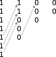
(a)

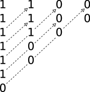
(b)

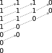
(c)

(d)

Figure 3: Sample run of the slope-sorting phase of 4-Wise Merging Network.

In the $i$-th iteration of the loop the values of columns $\bar{w}^{i}$, $\bar{x}^{i}$, $\bar{y}^{i}$ and $\bar{z}^{i}$ are obtained by sorting the results of the previous iteration in slope lines with decreasing slope rate. The sizes of the sorted prefix of the columns can also decrease in each iteration, but we would like to keep the $k$ largest input elements in that prefixes. In the following observation and lemma we define and formulate the basic properties of the column lengths after each iteration.

Observation 2.

Let $k_{1},\dots,k_{4}$ be as defined in Network 3. For each $i$, $0\leq i\leq\left\lceil\log(k_{1})\right\rceil$, let $c_{i}=\min(k_{3},\left\lfloor k/4\right\rfloor+h_{i})$, $b_{i}=\min(k_{2},c_{i}+h_{i})$ and $a_{i}=\min(k_{1},b_{i}+h_{i})$. Then we have: $k_{1}\geq a_{i}\geq b_{i}\geq c_{i}\geq\left\lfloor k/4\right\rfloor$ and the inequalities: $a_{i}-b_{i}\leq h_{i}$, $b_{i}-c_{i}\leq h_{i}$ and $c_{i}-\left\lfloor k/4\right\rfloor\leq h_{i}$ are true.

Proof.

From Observation 1.(1) we have $k_{1}\geq k_{2}\geq k_{3}\geq\left\lfloor k/4\right\rfloor$. It follows that $c_{i}\geq\left\lfloor k/4\right\rfloor$ and $b_{i}\geq\min(k_{3},\left\lfloor k/4\right\rfloor+h_{i})=c_{i}$ and $k_{1}\geq a_{i}\geq\min(k_{2},c_{i}+h_{i})=b_{i}$. Moreover, one can see that $c_{i}-\left\lfloor k/4\right\rfloor=\min(k_{3}-\left\lfloor k/4\right\rfloor,h_{i})\leq h_{i}$, $b_{i}-c_{i}=\min(k_{2}-c_{i},h_{i})\leq h_{i}$ and $a_{i}-b_{i}=\min(k_{1}-b_{i},h_{i})\leq h_{i}$, so we are done. ∎

Lemma 2.

Let $a_{i},b_{i},c_{i}$, $0\leq i\leq\left\lceil\log(k_{1})\right\rceil$, be as defined in Observation 2. Let $\check{w}^{i}=\textrm{pref}(a_{i},\bar{w}^{i})$, $\check{x}^{i}=\textrm{pref}(b_{i},\bar{z}^{i})$, $\check{y}^{i}=\textrm{pref}(c_{i},\bar{y}^{i})$ and $\check{z}^{i}=\bar{z}^{i}$. Then only the items in $\check{w}^{i}$, $\check{x}^{i}$, $\check{y}^{i}$ and $\check{z}^{i}$ take part in the $i$-th iteration of sorting operations in lines 8-14 of Network 3.

Proof.

An element of the vector $\bar{z}^{i}$, that is, $z^{i}_{j}$ is sorted in one of the lines 8–10 of Network 3, thus for all such $j$ that $1\leq j\leq k_{4}=\left\lfloor k/4\right\rfloor$. An element $y^{i}_{j}$ of $\bar{y}^{i}$ is sorted in lines 8–10 of the first inner loop and in lines 12–13 of the second inner loop. In the first three of those lines we have the bounds on $j$: $1+h_{i}\leq j\leq\min(k_{3},k_{4}+h_{i})$ and in the last three lines - the bounds: $1\leq j\leq\min(k_{3},h_{i})$. The sum of these two intervals is $1\leq j\leq min(k_{3},\left\lfloor k/4\right\rfloor+h_{i})=c_{i}$. Similarly, we can analyse the operations on $x^{i}_{j}$ in lines 8–10, 12–13 and 14. The range of $j$ is the sum of the following disjoint three intervals: $[1+2h_{i},\min(k_{2},k_{3}+h_{i},k_{4}+2h_{i})]$, $[1+h_{i},\min(k_{3}+h_{i},2h_{i})]$ and $[1,\min(k_{2},h_{i})]$ that give us the interval $[1,\min(k_{2},k_{3}+h_{1},k_{4}+2h_{i})]=[1,b_{i}]$ as their sum. The analysis of the range of $j$ used in the operations on $w^{i}_{j}$ in Network 3 can be done in the same way. ∎

The next lemma formulates the key invariants of the main loop in Network 3. They will be used in the proof of the main theorem in this section stating the merging properties of the network.

Lemma 3.

Let $\check{w}^{i}$, $\check{x}^{i}$, $\check{y}^{i}$ and $\check{z}^{i}$ be as defined in Lemma 2. Then for all $i$, $0\leq i\leq\left\lceil\log_{2}k_{1}\right\rceil$, after the $i$-th iteration of the while loop in Network 3 the sequences $\check{w}^{i},\check{x}^{i},\check{y}^{i},\check{z}^{i}$ are of the form $1^{p_{i}}0^{*}$, $1^{q_{i}}0^{*}$, $1^{r_{i}}0^{*}$ and $1^{s_{i}}0^{*}$, respectively, and:

$$p_{i}\geq q_{i}\geq r_{i}\geq s_{i},$$ (1)

$$p_{i}-q_{i}\leq h_{i}\textrm{~{}and~{}}q_{i}-r_{i}\leq h_{i}\textrm{~{}and~{}}r_{i}-s_{i}\leq h_{i},$$ (2)

$$p_{i}+q_{i}+r_{i}+s_{i}\geq\min(k,p_{0}+q_{0}+r_{0}+s_{0}).$$ (3)

Proof.

By induction. At the beginning we have $h_{0}\geq k_{1}\geq k_{2}\geq k3\geq k4=\left\lfloor k/4\right\rfloor$ and therefore $\check{w}^{0}=\bar{w}$, $\check{x}^{0}=\bar{x}$, $\check{y}^{0}=\bar{y}$ and $\check{z}^{0}=\bar{z})$. All four sequences $\bar{w},\bar{x},\bar{y},\bar{z}$ are sorted (by Definition 4), thus, they are of the form $1^{p_{0}}0^{*}$, $1^{q_{0}}0^{*}$, $1^{r_{0}}0^{*}$, and $1^{s_{0}}0^{*}$ respectively. By Definition 4.(2), for each pair of sequences: $(\bar{w}_{1..k_{2}},\bar{x})$, $(\bar{x}_{1..k_{3}},\bar{y})$ and $(\bar{y}_{1..k_{4}},\bar{z})$, if there is a 1 on the $j$ position in the right sequence, it must be a corresponding 1 on the same position in the left one. Therefore, we have: $p_{0}\geq q_{0}\geq r_{0}\geq s_{0}\geq 0$. Moreover, $p_{0}-q_{0}\leq p_{0}\leq k_{1}\leq h_{0}$, $q_{0}-r_{0}\leq q_{0}\leq k_{2}\leq h_{0}$ and $r_{0}-s_{0}\leq r_{0}\leq k_{3}\leq h_{0}$. Finally, $p_{0}+q_{0}+r_{0}+s_{0}\geq\min(k,p_{0}+q_{0}+r_{0}+s_{0})$, thus the lemma holds for $i=0$.

In the inductive step $i>0$ observe that the elements of $\check{w}^{i}$, $\check{x}^{i}$, $\check{y}^{i}$ and $\check{z}^{i}$ are defined by the sort operations over the elements with the same indices from vectors $\check{w}^{i-1}$, $\check{x}^{i-1}$, $\check{y}^{i-1}$ and $\check{z}^{i-1}$. This means that the values of $w^{i-1}_{a_{i}+1,\dots,a_{i+1}}$, $x^{i-1}_{b_{i}+1,\dots,b_{i+1}}$ and $y^{i-1}_{c_{i}+1,\dots,c_{i+1}}$ are not used in the $i$-th iteration. Therefore, the numbers of 1’s in columns that are sorted in the $i$-th iteration are defined by values: $p^{\prime}_{i-1}=\min(a_{i},p_{i-1})$, $q^{\prime}_{i-1}=\min(b_{i},q_{i-1})$, $q^{\prime}_{i-1}=\min(c_{i},r_{i-1})$ and $s^{\prime}_{i-1}=s_{i-1}$. In the following we will prove that the numbers with primes have the same properties as those without them.

$$p^{\prime}_{i-1}\geq q^{\prime}_{i-1}\geq r^{\prime}_{i-1}\geq s^{\prime}_{i-1},$$ (4)

$$p^{\prime}_{i-1}-q^{\prime}_{i-1}\leq h_{i-1}\textrm{~{}and~{}}q^{\prime}_{i-1}-r^{\prime}_{i-1}\leq h_{i-1}\textrm{~{}and~{}}r^{\prime}_{i-1}-s^{\prime}_{i-1}\leq h_{i-1},$$ (5)

$$p^{\prime}_{i-1}+q^{\prime}_{i-1}+r^{\prime}_{i-1}+s^{\prime}_{i-1}\geq\min(k,p_{i-1}+q_{i-1}+r_{i-1}+s_{i-1}).$$ (6)

The proofs of inequalities in Eq. 4 are quite direct and follow from the monotonicity of $\min$. For example, we can observe that $p^{\prime}_{i-1}=\min(a_{i},p_{i-1})\geq\min(b_{i},q_{i-1})=q^{\prime}_{i-1}$, since we have $a_{i}\geq b_{i}$ and $p_{i-1}\geq q_{i-1}$, by Observation 2 and the induction hypothesis. The others can be shown in the same way.

Let us now prove one of the inequalities of Eq. (5), say, the second one. We have $q^{\prime}_{i-1}-r^{\prime}_{i-1}=\min(b_{i},q_{i-1})-\min(c_{i},r_{i-1})\leq\min(c_{i}+h_{i},r_{i-1}+h_{i-1})-\min(c_{i},r_{i-1})\leq h_{i-1}$, by Observation 2, the fact that $h_{i-1}=2h_{i}$ and the induction hypothesis. The proofs of the others are similar.

The proof of Eq. (6) is only needed if at least one of the following inequalities are true: $p^{\prime}_{i-1}<p_{i-1}$, $q^{\prime}_{i-1}<q_{i-1}$ or $r^{\prime}_{i-1}<r_{i-1}$. Obviously, the inequalities are equivalent to $a_{i}<p_{i-1}$, $b_{i}<q_{i-1}$ and $c_{i}<r_{i-1}$, respectively. Therefore, to prove Eq. 6 we consider now three separate cases: (1) $a_{i}\geq p_{i-1}$ and $b_{i}\geq q_{i-1}$ and $c_{i}<r_{i-1}$, (2) $a_{i}\geq p_{i-1}$ and $b_{i}<q_{i-1}$ and (3) $a_{i}<p_{i-1}$.

In the case (1) we have $p^{\prime}_{i-1}=p_{i-1}$, $q^{\prime}_{i-1}=q_{i-1}$ and $r^{\prime}_{i-1}=c_{i}=\min(k_{3},h_{i}+\left\lfloor k/4\right\rfloor)<r_{i-1}\leq q_{i-1}\leq p_{i-1}$. It follows that $p^{\prime}_{i-1}+q^{\prime}_{i-1}+r^{\prime}_{i-1}=p_{i-1}+q_{i-1}+c_{i}\geq c_{i}+1+c_{i}+1+c_{i}=3c_{i}+2$. Since $k_{3}\geq r_{i-1}\geq c_{i}+1=\min(k_{3},\left\lfloor k/4\right\rfloor+h_{i})+1$, we can observe that $c_{i}$ must be equal to $\left\lfloor k/4\right\rfloor+h_{i}$. In addition, by the induction hypothesis we have $s_{i-1}\geq r_{i-1}-h_{i-1}\geq c_{i}+1-2h_{i}$. Merging those facts we can conclude that $p^{\prime}_{i-1}+q^{\prime}_{i-1}+r^{\prime}_{i-1}+s^{\prime}_{i-1}\geq 4c_{i}+3-2h_{i}=4\left\lfloor k/4\right\rfloor+4h_{i}+3-2h_{i}\geq k$, so we are done in this case.

In the case (2) we have $p^{\prime}_{i-1}=p_{i-1}$ and $q^{\prime}_{i-1}=b_{i}=\min(k_{2},c_{i}+h_{i})<q_{i-1}\leq p_{i-1}$. It follows that $p^{\prime}_{i-1}+q^{\prime}_{i-1}\geq 2b_{i}+1$. Since $k_{2}\geq q_{i-1}\geq b_{i}+1=\min(k_{2},c_{i}+h_{i})+1$, we can observe that $b_{i}$ must be equal to $c_{i}+h_{i}$. In addition, by the induction hypothesis and Observation 2, we can bound $r^{\prime}_{i-1}$ as $r^{\prime}_{i-1}=\min(c_{i},r_{i-1})\geq\min(b_{i}-h_{i},q_{i-1}-h_{i-1})\geq b_{i}+1-2h_{i}$. Therefore, $p^{\prime}_{i-1}+q^{\prime}_{i-1}+r^{\prime}_{i-1}\geq 3b_{i}+2-2h_{i}=3c_{i}+2+h_{i}$. Since $c_{i}$ is defined as $\min(k_{3},\left\lfloor k/4\right\rfloor+h_{i})$, we have to consider two subcases of the possible value of $c_{i}$. If $c_{i}=k_{3}\leq\left\lfloor k/4\right\rfloor+h_{i}$, then we have $k_{2}\geq q_{i-1}\geq b_{i}+1=c_{i}+h_{i}+1\geq k_{3}+2$. By Observation 1.(3), $k_{3}$ must be equal to $\left\lfloor k/3\right\rfloor$, thus $3c_{i}+2=3k_{3}+2\geq k$, and we are done. Otherwise, we have $c_{i}=\left\lfloor k/4\right\rfloor+h_{i}$ and since $s^{\prime}_{i-1}=s_{i-1}\geq r_{i-1}-h_{i-1}\geq b_{i}+1-4h_{i}=c_{i}+1-3h_{i}$, we can conclude that $p^{\prime}_{i-1}+q^{\prime}_{i-1}+r^{\prime}_{i-1}+s^{\prime}_{i-1}\geq 4c_{i}+3-2h_{i}=4\left\lfloor k/4\right\rfloor+3+2h_{i}\geq k$.

The last case $a_{i}<p_{i-1}$ can be proved be the similar arguments. Having Eqs. (4.5,6), we can start proving the inequalities from the lemma. Observe that in Network 4 the values of vectors $\bar{w}^{i}$, $\bar{x}^{i}$, $\bar{y}^{i}$ and $\bar{z}^{i}$ are defined with the help of three types of sorters: $\textit{sort}^{4}$, $\textit{sort}^{3}$ and $\textit{sort}^{2}$. The smaller sorters are used, when the corresponding index is out of the range and an input item is not available. In the following analysis we would like to deal only with $\textit{sort}^{4}$ and in the case of smaller sorters we extend artificially their inputs and outputs with 1’s at the left end and 0’s at the right end. For example, in line 18 we have $\langle y^{i}_{j},x^{i}_{j+h_{i}}\rangle\leftarrow\textit{sort}^{2}(y^{i-1}_{j},x^{i-1}_{j+h_{i}})$ and we can analyse this operation as $\langle 1,y^{i}_{j},x^{i}_{j+h_{i}},0\rangle\leftarrow\textit{sort}^{4}(1,y^{i-1}_{j},x^{i-1}_{j+h_{i}},0)$. The 0 input corresponds to the element of $\bar{w}^{i-1}$ with index $j+2h_{i}$, where $j+2h_{i}>k_{1}\geq a_{i}$, and the 1 input corresponds to the element of $\bar{z}^{i-1}$ with index $j-h_{i}$, where $j-h_{i}<0$. A similar situation is in lines 10, 12, 16 and 22, where $\textit{sort}^{2}$ and $\textit{sort}^{3}$ are used. Therefore, in the following we assume that elements of input sequences $\bar{w}^{i-1}$, $\bar{x}^{i-1}$, $\bar{y}^{i-1}$ and $\bar{z}^{i-1}$ with negative indices are equal to 1 and elements of the inputs with indices above $a_{i}$, $b_{i}$, $c_{i}$ and $\left\lfloor k/4\right\rfloor$, respectively, are equal to 0. This assumption does not break the monotonicity of the sequences and we also have the property that $w^{i-1}_{j}=1$ if and only if $j\leq p^{\prime}_{j-1}$ (and similar ones for $\bar{x}^{i-1}$ and $q^{\prime}_{i-1}$, and so on).

It should be clear now that, under the assumption above, we have:

$$w^{i}_{j}= \min(w^{i-1}_{j},x^{i-1}_{j-h_{i}},y^{i-1}_{j-2h_{i}},z^{i-1}_{j-3h_{i}}) \textrm{~{}for~{}}1\leq j\leq a_{i},$$ (7a)

$$x^{i}_{j}= \textrm{2nd}(w^{i-1}_{j+h_{i}},x^{i-1}_{j},y^{i-1}_{j-h_{i}},z^{i-1}_{j-2h_{i}}) \textrm{~{}for~{}}1\leq j\leq b_{i},$$ (7b)

$$y^{i}_{j}= \textrm{3rd}(w^{i-1}_{j+2h_{i}},x^{i-1}_{j+h_{i}},y^{i-1}_{j},z^{i-1}_{j-h_{i}}) \textrm{~{}for~{}}1\leq j\leq c_{i},$$ (7c)

$$z^{i}_{j}= \max(w^{i-1}_{j+3h_{i}},x^{i-1}_{j+2h_{i}},y^{i-1}_{j+h_{i}},z^{i-1}_{j}) \textrm{~{}for~{}}1\leq j\leq\left\lfloor k/4\right\rfloor,$$ (7d)

where 2nd and 3rd denote the second and the third smallest element of its input, respectively. Since the functions $\min$, 2nd, 3rd and $\max$ are monotone and the input sequences are monotone. we can conclude that $w^{i}_{j}\geq w^{i}_{j+1}$, $x^{i}_{j}\geq x^{i}_{j+1}$, $y^{i}_{j}\geq y^{i}_{j+1}$ and $z^{i}_{j}\geq z^{i}_{j+1}$. Let $p_{i}$, $q_{i}$, $r_{i}$ and $s_{i}$ denote the numbers of 1’s in them. Clearly, we have $p_{i}+q_{i}+r_{i}+s_{i}=p^{\prime}_{i-1}+q^{\prime}_{i-1}+r^{\prime}_{i-1}+s^{\prime}_{i-1}$, thus $p_{i}+q_{i}+r_{i}+s_{i}\geq\min(k,p_{i-1}+q_{i-1}+r_{i-1}+s_{i-1})\geq\min(k,p_{0}+q_{0}+r_{0}+s_{0})$, by the induction hypothesis. Thus. we have proved monotonicity of $\bar{w}^{i}$, $\bar{x}^{i}$, $\bar{y}^{i}$ and $\bar{z}^{i}$ and that Eq. (3) holds.

To prove Eq. (2) we would like to show that $p_{i}-h_{i}\leq q_{i}$, $q_{i}-h_{i}\leq r_{i}$, $r_{i}-h_{i}\leq s_{i}$, that is, that the following equalities are true: $x^{i}_{p_{i}-h_{i}}=1$, $y^{i}_{q_{i}-h_{i}}=1$ and $z^{i}_{r_{i}-h_{i}}=1$. The first equality follows from the fact that $w^{i}_{p_{i}}=1$ and $w^{i}_{p_{i}}\leq x^{i}_{p_{i}-h_{i}}$, because they are output in this order by a single sort operation. The other two equalities can be shown by the similar arguments.

The last equation we have to prove is (1). By the induction hypothesis and our assumption we have $w^{i-1}_{j}\geq x^{i-1}_{j}\geq y^{i-1}_{j}\geq z^{i-1}_{j}$, for any $j$. We know also that the vectors are non-increasing. We use these facts to show that $w^{i}_{q_{i}}=1$, which is equivalent to $p_{i}\geq q_{i}$. Since $w^{i}_{q_{i}}=\min(w^{i-1}_{q_{i}},x^{i-1}_{q_{i}-h_{i}},y^{i-1}_{q_{i}-2h_{i}},z^{i-1}_{q_{i}-3h_{i}})$, we have to prove that all the arguments of the $\min$ function are 1’s. From the definition of $q_{i}$ we have $1=x^{i}_{q_{i}}=\textrm{2nd}(w^{i-1}_{q_{i}+h_{i}},x^{i-1}_{q_{i}},y^{i-1}_{q_{i}-h_{i}},z^{i-1}_{q_{i}-2h_{i}})$, thus the maximum of any pair of arguments of 2nd must be 1. Now we can see that $w^{i-1}_{q_{i}}\geq\max(w^{i-1}_{q_{i}+h_{i}},x^{i-1}_{q_{i}})\geq 1$, $x^{i-1}_{q_{i}-h_{i}}\geq\max(x^{i-1}_{q_{i}},y^{i-1}_{q_{i}-h_{i}})\geq 1$, $y^{i-1}_{q_{i}-2h_{i}}\geq\max(y^{i-1}_{q_{i}-h_{i}},z^{i-1}_{q_{i}-2h_{i}})\geq 1$ and $z^{i-1}_{q_{i}-3h_{i}}\geq\max(y^{i-1}_{q_{i}-h_{i}},z^{i-1}_{q_{i}-2h_{i}})\geq 1$. In the last inequality we use the fact that for any $j$ it is true that $z^{i-1}_{j-2h_{i}}\geq y^{i-1}_{j}$ (because $r^{\prime}_{i-1}-2h_{i}\leq s^{\prime}_{i-1}$, by Eq. (5)). Thus, $w^{i}_{q_{i}}$ must be 1 and we are done. The other two inequalities can be proved in the similar way with the help of two additional relations: $x^{i-1}_{j-2h_{i}}\geq w^{i-1}_{j}$ and $y^{i-1}_{j-2h_{i}}\geq x^{i-1}_{j}$, which follows from the induction hypothesis. ∎

Theorem 4.1.

The output of Network 3 is top $k$ sorted.

Proof.

The zip operation outputs its input vectors in the row-major order. By Eq. (3) of Lemma 3, we know that elements in the $out$ sequence are dominated by the $k$ largest elements in the output vectors of the main loop. From the order diagram given in Fig. 2 it follows that $\langle y_{i-1},\max(z_{i-1},w_{j+1}),w_{j},x_{j}\rangle$ dominates $\langle y_{i},z_{i},\min(z_{i-1},w_{j+1}),x_{i+1}\rangle$, thus, after the sorting operations in lines 15–16, the values will appear in the row-major order. The two special cases, where the whole sequence of four elements is not available for the $\textit{sort}^{4}$ operation, are covered by lines 17 and 18. If the vector $\check{x}^{i}$ does not have the element with index $k_{4}+1$, then just 3 elements are sorted in line 17. If $k\bmod 4=3$ then the element $y_{k_{4}+1}$ is the last one in desired order, but the vector $\check{z}^{i}$ does not have the element with index $k_{4}+1$, so the network must sort just 2 elements in line 18. Note that in the first $\left\lfloor k/4\right\rfloor$ rows we have $4\left\lfloor k/4\right\rfloor$ elements of the top $k$ ones, so the values of $k-4\left\lfloor k/4\right\rfloor$ leftmost elements in the row $k_{4}+1$ should be corrected. ∎

4.2 4-Odd-Even Merging Networks

In this subsection the second merging algorithm for four columns is presented (Network 5). The input to the procedure is $\langle pref(k_{1},\bar{y}^{1}),\dots,pref(k_{m},\bar{y}^{m})\rangle$, where each $\bar{y}^{i}$ is the output of the recursive call in Network 2. Again, the goal is to put the $k$ largest elements in top rows. It is done by splitting each input sequence into two parts, one containing elements of odd index, the other containing elements of even index. Odd sequences and even sequences are then recursively merged (lines 7–8). The resulting sequences are again split into odd and even parts, and combined using auxiliary Network 4 (lines 9–10). Lastly, the combine operation is used again (line 11) to get the top $k$ sorted sequence.

Our network is the generalization of the classic Odd-Even Merging Network by Batcher [6]. Network 4 is the standard combine operation of the Odd-Even Merging Network, but with smaller number of comparators, since our network is the selection network. For more information on these classes of networks and to see examples, see [13].

Definition 9.

A binary sequence $\bar{r}$ is top $k^{\prime}$ full if it is of the form $1^{k^{\prime}}\bar{r}^{\prime}$, where $\bar{r}^{\prime}\in\{0,1\}^{|\bar{r}|-k^{\prime}}$.

Network 4 $oe\_combine^{s}_{k}$

1:A pair of sequences $\langle\bar{x},\bar{y}\rangle$, where $k\leq s=|\bar{x}|+|\bar{y}|$.

2:$\bar{z}\leftarrow\textrm{zip}(\bar{x},\bar{y})$

3:for all $i\in\{1,\dots,\left\lfloor\min(k,|\bar{z}|-1)/2\right\rfloor\}$ do

4:     $\textit{sort}^{2}(z_{2i},z_{2i+1})$

5:return $\bar{z}$

Observation 3.

Let $K,k,l\in\mathbb{N}$ and $K\geq k+l$ and $0\leq l-k\leq 2$. If $\bar{a}$ is top $l$ full and $\bar{b}$ is top $k$ full then $oe\_combine^{|a|+|b|}_{K}(\bar{a},\bar{b})$ is top $l+k$ full.

Proof.

If $l\in\{k,k+1\}$ or $b_{k+1}=1$, then $oe\_combine^{|a|+|b|}_{K}(\bar{a},\bar{b})$ is top $l+k$ full due to the zip operation in line 1 (notice that additional sorting is not needed). If $l=k+2$ and $b_{k+1}=0$, then after the zip operation in line 1, the sequence $\bar{z}$ is of the form $1^{2k+1}01\{0,1\}^{*}$. Since $K\geq k+l=2k+2$, the elements $\langle z_{2k+2},z_{2k+3}\rangle=\langle 0,1\rangle$ will be sorted in line 3. Therefore $\bar{z}$ will be of the form $1^{2k+2}\{0,1\}^{*}$, so $\bar{z}$ is top $l+k$ full. ∎

Network 5 $4oe\_merge^{s}_{k}$

1:A tuple of top $k$ sorted sequences $\langle\bar{w},\bar{x},\bar{y},\bar{z}\rangle$, where $s=|\bar{w}|+|\bar{x}|+|\bar{y}|+|\bar{z}|$, $|\bar{w}|\geq|\bar{x}|\geq|\bar{y}|\geq|\bar{z}|$ and $k\geq 1$.

2:$k_{1}=|\bar{w}|$;   $k_{2}=|\bar{x}|$;   $k_{3}=|\bar{y}|$;   $k_{4}=|\bar{z}|$

3:if $k_{2}=0$ then return $\bar{w}$

4:if $k_{1}=1$ then

5:     $\bar{a}\leftarrow\textrm{zip}(\bar{w},\bar{x},\bar{y},\bar{z})$

6:     return $\textit{sort}^{|\bar{a}|}(\bar{a})$

7:$sa=\left\lceil k_{1}/2\right\rceil+\left\lceil k_{2}/2\right\rceil+\left\lceil k_{3}/2\right\rceil+\left\lceil k_{4}/2\right\rceil$;   $sb=\left\lfloor k_{1}/2\right\rfloor+\left\lfloor k_{2}/2\right\rfloor+\left\lfloor k_{3}/2\right\rfloor+\left\lfloor k_{4}/2\right\rfloor$

8:$\bar{a}\leftarrow 4oe\_merge^{sa}_{\min(sa,\left\lfloor k/2\right\rfloor+2)}(\bar{w}_{\textit{odd}},\bar{x}_{\textit{odd}},\bar{y}_{\textit{odd}},\bar{z}_{\textit{odd}})$ $\triangleright$ Recursive calls.

9:$\bar{b}\leftarrow 4oe\_merge^{sb}_{\min(sb,\left\lfloor k/2\right\rfloor)}(\bar{w}_{\textit{even}},\bar{x}_{\textit{even}},\bar{y}_{\textit{even}},\bar{z}_{\textit{even}})$

10:$\bar{c}\leftarrow oe\_combine_{\left\lfloor k/2\right\rfloor+1}(\bar{a}_{\textit{odd}},\bar{b}_{\textit{odd}})$

11:$\bar{d}\leftarrow oe\_combine_{\left\lfloor k/2\right\rfloor}(\bar{a}_{\textit{even}},\bar{b}_{\textit{even}})$

12:return $oe\_combine_{k}(\bar{c},\bar{d})$ $\triangleright$ The output is top $k$ sorted.

Observation 4.

If $\bar{x}$ is a sorted sequence, then $|\bar{x}_{\textit{odd}}|_{1}-|\bar{x}_{\textit{even}}|_{1}\leq 1$.

Lemma 4.

Let $k,k^{\prime}\in\mathbb{N}$ and $k^{\prime}\leq k$. If $\langle\bar{w},\bar{x},\bar{y},\bar{z}\rangle$ is a top $k^{\prime}$ sorted tuple such that $k\leq s=|\bar{w}|+|\bar{x}|+|\bar{y}|+|\bar{z}|$ and $|\bar{w}|\geq|\bar{x}|\geq|\bar{y}|\geq|\bar{z}|$, then $4oe\_merge^{s}_{k}(\bar{w},\bar{x},\bar{y},\bar{z})$ is top $k^{\prime}$ sorted.

Proof.

By induction on $(k^{\prime},s)$. First we introduce the schema of the proof, as it has many base cases:

1. When $k^{\prime}\leq s=1$ or $k_{1}=1$.

2. When $k^{\prime}=s$ and $k_{1}\geq 2$.

3. When $k^{\prime}=1$.

4. When $k^{\prime}=2$.

After that we will prove the inductive step. Notice that we needed to include cases 2 and 4 in the base step, because inductive step is only viable when $\left\lfloor k^{\prime}/2\right\rfloor+2\leq k^{\prime}$, which is when $k^{\prime}\geq 3$.

Ad. 1. If $k^{\prime}\leq s=1$, then from $k_{1}\geq k_{2}\geq k_{3}\geq k_{4}$ we get that $k_{1}=1$ and $k_{2}=0$. Therefore $\bar{w}$ is the only non-empty input sequence and it consists of only one element, therefore it is sorted and the algorithm terminates on line 2. If $k_{1}=1$, then from $k_{1}\geq k_{2}\geq k_{3}\geq k_{4}$ we get that each input sequence has at most one element. Therefore using sorter of order at most 4 gives the desired result (lines 4–5).

Ad. 2. If $k^{\prime}=s$, then $k=s$. Assume that $k_{1}\geq 2$. We prove this case by induction on $s$. Base case is covered by $(1)$. Take any $s>1$ and assume that for any $s^{\prime}<s$, the lemma holds. Consider the execution of $4oe\_merge^{s}_{s}(\bar{w},\bar{x},\bar{y},\bar{z})$. Each input sequence is top $s$ sorted, therefore they are sorted. Which means that $\langle\bar{w}_{\textit{odd}},\bar{x}_{\textit{odd}},\bar{y}_{\textit{odd}},\bar{z}_{\textit{odd}}\rangle$ and $\langle\bar{w}_{\textit{even}},\bar{x}_{\textit{even}},\bar{y}_{\textit{even}},\bar{z}_{\textit{even}}\rangle$ are also sorted. Since $\min(sa,\left\lfloor s/2\right\rfloor+2)=sa$, $\min(sb,\left\lfloor s/2\right\rfloor)=sb$, $sa<s$ (because $k_{1}\geq 2$) and $sb<s$ we can use the induction hypothesis to get that $\bar{a}$ is top $sa$ sorted and $\bar{b}$ is top $sb$ sorted. Since $|\bar{a}|=sa$ and $|\bar{b}|=sb$ we get that $\bar{a}$ and $\bar{b}$ are sorted. Using Observation 4 on the input sequences we also get that $|\bar{a}|_{1}-|\bar{b}|_{1}\leq 4$. Therefore sequences $\bar{a}_{\textit{odd}},\bar{b}_{\textit{odd}},\bar{a}_{\textit{even}},\bar{b}_{\textit{even}}$ are sorted and $|\bar{a}_{\textit{odd}}|_{1}-|\bar{b}_{\textit{odd}}|_{1}\leq 2$ and $|\bar{a}_{\textit{even}}|_{1}-|\bar{b}_{\textit{even}}|_{1}\leq 2$. It is easy to check that $|\bar{a}_{\textit{odd}}|_{1}+|\bar{b}_{\textit{odd}}|_{1}\leq\left\lceil sa/2\right\rceil+\left\lceil sb/2\right\rceil\leq\left\lceil sa/2\right\rceil+\left\lfloor sb/2\right\rfloor+1=\left\lceil s/4\right\rceil+\left\lfloor s/4\right\rfloor+1\leq\left\lfloor s/2\right\rfloor+1$, (for $s>1$). Similarly we get $|\bar{a}_{\textit{even}}|_{1}+|\bar{b}_{\textit{even}}|_{1}\leq\left\lfloor sa/2\right\rfloor+\left\lfloor sb/2\right\rfloor\leq\left\lceil sa/2\right\rceil+\left\lfloor sb/2\right\rfloor=\left\lceil s/4\right\rceil+\left\lfloor s/4\right\rfloor\leq\left\lfloor s/2\right\rfloor$, (for $s>1$). Therefore from Observation 3 we get that $\bar{c}$ is top $|\bar{a}_{\textit{odd}}|_{1}+|\bar{b}_{\textit{odd}}|_{1}$ full and $\bar{d}$ is top $|\bar{a}_{\textit{even}}|_{1}+|\bar{b}_{\textit{even}}|_{1}$ full. Also since $\bar{a}_{\textit{odd}},\bar{b}_{\textit{odd}},\bar{a}_{\textit{even}},\bar{b}_{\textit{even}}$ were sorted, $\bar{c}$ and $\bar{d}$ are also sorted. Using Observation 4 we get that $|\bar{c}|_{1}-|\bar{d}|_{1}=|\bar{a}_{\textit{odd}}|_{1}+|\bar{b}_{\textit{odd}}|_{1}-|\bar{a}_{\textit{even}}|_{1}-|\bar{b}_{\textit{even}}|_{1}\leq 2$. Also $|\bar{c}|_{1}+|\bar{d}|_{1}\leq\left\lceil sa/2\right\rceil+\left\lceil sb/2\right\rceil+\left\lfloor sa/2\right\rfloor+\left\lfloor sb/2\right\rfloor=sa+sb=s$. Therefore using Observation 3 we get that the sequence returned in line 11 is top $|\bar{c}|_{1}+|\bar{d}|_{1}$ full and it is sorted, since $\bar{c}$ and $\bar{d}$ were sorted. This completes the inductive step and this case.

Ad. 3. Let $k\geq k^{\prime}=1$. We prove this case by induction on $s$. Assume $s>1$ and $k_{1}\geq 2$ (the other cases are covered by $(1)$). Consider two sub-cases:

$(i)$. $|\bar{w}::\bar{x}::\bar{y}::\bar{z}|_{1}=0$. Therefore output of the algorithm is of the form $0^{*}$, so it is top $k^{\prime}$ sorted.

$(ii)$. $|\bar{w}::\bar{x}::\bar{y}::\bar{z}|_{1}>0$. Without loss of generality assume that $|\bar{w}|_{1}>0$, and because it is top $k^{\prime}$ sorted, we get that $w_{1}=1$. Because of that $w^{\textit{odd}}_{1}=1$ and since $k_{1}\geq 2$, we get that $sa<s$, so we can use induction hypothesis to get that $\bar{a}$ is top $\left\lceil k^{\prime}/2\right\rceil=1$ sorted and $a_{1}=1$. From this we get that $a^{\textit{odd}}_{1}=1$, therefore $c_{1}=1$. From this we conclude that the output in line 11 is of the form $1\{0,1\}^{*}$, so it is top $k^{\prime}$ sorted.

Ad. 4. Let $k\geq k^{\prime}=2$. Assume $s>2$ and $k_{1}\geq 2$ (the other cases are covered by $(1)$ and $(2)$). From our assumptions $\left\lceil k^{\prime}/2\right\rceil=\left\lfloor k^{\prime}/2\right\rfloor=1$. Therefore from case $(3)$ we get that $\bar{a}$ and $\bar{b}$ are top 1 sorted. Notice that $\left\lfloor k/2\right\rfloor+1\geq 2$ and consider $\langle a_{1},b_{1}\rangle,\langle a_{2},b_{2}\rangle\in\{\langle 0,0\rangle,\langle 1,0\rangle,\langle 1,1\rangle\}$. Using Observation 3, in all possible cases $\bar{c}$ is top 2 sorted (regardless of the value of $a_{3}$) and $\bar{d}$ is top 1 sorted. We can now consider all possible cases for values of $c_{1},c_{2}$ and $d_{1}$ and using Observation 3 again, conclude that the sequence returned in line 11 is top $2=k^{\prime}$ sorted.

We can finally prove the induction step. Assume $s\geq k\geq k^{\prime}>2$ and $k_{1}\geq 2$. Consider three cases:

(i) One of the input sequences (say $\bar{w}$) is top $k^{\prime}$ full. Therefore $\bar{w}_{\textit{odd}}$ is top $\left\lceil k^{\prime}/2\right\rceil$ full and $\bar{w}_{\textit{even}}$ is top $\left\lfloor k^{\prime}/2\right\rfloor$ full. Also since $s\geq k^{\prime}>2$ and $k_{1}\geq 2$ we get that $sa<s$, $sb<s$ and $\left\lfloor k^{\prime}/2\right\rfloor+2\leq k^{\prime}$. Therefore we can use induction hypothesis to get that $\bar{a}$ is top $\left\lceil k^{\prime}/2\right\rceil$ full and $\bar{b}$ is top $\left\lfloor k^{\prime}/2\right\rfloor$ full. Therefore $\bar{a}_{\textit{odd}}$ is top $\left\lceil\left\lceil k^{\prime}/2\right\rceil/2\right\rceil$ full,$\bar{a}_{\textit{even}}$ is top $\left\lfloor\left\lceil k^{\prime}/2\right\rceil/2\right\rfloor$ full, $\bar{b}_{\textit{odd}}$ is top $\left\lceil\left\lfloor k^{\prime}/2\right\rfloor/2\right\rceil$ full and $\bar{b}_{\textit{even}}$ is top $\left\lfloor\left\lfloor k^{\prime}/2\right\rfloor/2\right\rfloor$ full. Let $q=\left\lceil\left\lfloor k^{\prime}/2\right\rfloor/2\right\rceil+\left\lceil\left\lfloor k^{\prime}/2\right\rfloor/2\right\rceil$ and $r=\left\lfloor\left\lceil k^{\prime}/2\right\rceil/2\right\rfloor+\left\lfloor\left\lfloor k^{\prime}/2\right\rfloor/2\right\rfloor$. Notice that $q\leq\left\lfloor k^{\prime}/2\right\rfloor+1$ and $r\leq\left\lfloor k^{\prime}/2\right\rfloor$ (for $k^{\prime}\geq 2$). Furthermore, $0\leq\left\lceil\left\lceil k^{\prime}/2\right\rceil/2\right\rceil-\left\lceil\left\lfloor k^{\prime}/2\right\rfloor/2\right\rceil\leq 1$ and $0\leq\left\lfloor\left\lceil k^{\prime}/2\right\rceil/2\right\rfloor-\left\lfloor\left\lfloor k^{\prime}/2\right\rfloor/2\right\rfloor\leq 1$. Hence we can use Observation 3 to get that $\bar{c}$ is top $q$ full and $\bar{d}$ is top $r$ full. It is easy to check that $0\leq q-r\leq 2$ and $q+r=k^{\prime}$, therefore we can use Observation 3 again and we can conclude that the last combine operation (line 11) will return top $k^{\prime}$ sorted sequence, therefore this case is done.

(ii) All input sequences are of the form $1^{j}0^{*}$, where $j<k^{\prime}$, and $I=|\bar{w}::\bar{x}::\bar{y}::\bar{z}|_{1}\leq k^{\prime}$. Since $s\geq k^{\prime}>2$ and $k_{1}\geq 2$ we get that $sa<s$, $sb<s$ and $\left\lfloor k^{\prime}/2\right\rfloor+2\leq k^{\prime}$. Therefore using induction hypothesis we get that $\bar{a}$ is of the form $1^{q}0^{*}$ and $\bar{b}$ is of the form $1^{r}0^{*}$, where $q+r=I$. Furthermore, applying Observation 4 to all input sequences we get that $0\leq q-r\leq 4$. Which means that $\bar{a}_{\textit{odd}},\bar{a}_{\textit{even}},\bar{b}_{\textit{odd}},\bar{b}_{\textit{even}}$ are all sorted and of the form $1^{\left\lceil q/2\right\rceil}0^{*}$, $1^{\left\lfloor q/2\right\rfloor}0^{*}$, $1^{\left\lceil r/2\right\rceil}0^{*}$, $1^{\left\lfloor r/2\right\rfloor}0^{*}$ respectively, also $0\leq|\bar{a}_{\textit{odd}}|_{1}-|\bar{b}_{\textit{odd}}|_{1}=\left\lceil q/2\right\rceil-\left\lceil r/2\right\rceil\leq 2$ and $0\leq|\bar{a}_{\textit{even}}|_{1}-|\bar{b}_{\textit{even}}|_{1}=\left\lfloor q/2\right\rfloor-\left\lfloor r/2\right\rfloor\leq 2$. Using Observation 3 we get that $\bar{c}$ is top $\left\lceil q/2\right\rceil+\left\lceil r/2\right\rceil$ full and $\bar{d}$ is top $\left\lfloor q/2\right\rfloor+\left\lfloor r/2\right\rfloor$ full. Moreover, $0\leq|\bar{c}|_{1}-|\bar{d}|_{1}=\left\lceil q/2\right\rceil+\left\lceil r/2\right\rceil-\left\lfloor q/2\right\rfloor-\left\lfloor r/2\right\rfloor\leq 2$, therefore using Observation 3 again we conclude that the returned sequence (in line 11) is top $q+r$ full, and since $q+r=I<k^{\prime}$, then the returned sequence is of the form $1^{I}0^{*}$, so it is also top $k^{\prime}$ sorted.

(iii) All input sequences are of the form $1^{j}0^{*}$, where $j<k^{\prime}$, and $I=|\bar{w}::\bar{x}::\bar{y}::\bar{z}|_{1}>k^{\prime}$. Since $s\geq k^{\prime}>2$ and $k_{1}\geq 2$ we get that $sa<s$, $sb<s$ and $\left\lfloor k^{\prime}/2\right\rfloor+2\leq k^{\prime}$. Therefore we can use induction hypothesis to get that $\bar{a}$ is top $\left\lfloor k^{\prime}/2\right\rfloor+2$ sorted and $\bar{b}$ is top $\left\lfloor k^{\prime}/2\right\rfloor$ sorted. Applying Observation 4 to all input sequences we get that $0\leq|\bar{a}|_{1}-|\bar{b}|_{1}\leq 4$, in particular, $|\bar{a}|_{1}\geq|\bar{b}|_{1}$. Let $q=|a_{1\dots\left\lfloor k^{\prime}/2\right\rfloor+2}|_{1}$ and $r=|b_{1\dots\left\lfloor k^{\prime}/2\right\rfloor}|_{1}$. Furthermore, either $\bar{a}$ is top $\left\lfloor k^{\prime}/2\right\rfloor+2$ full or $\bar{b}$ is top $\left\lfloor k^{\prime}/2\right\rfloor$ full. Otherwise $a_{\left\lfloor k^{\prime}/2\right\rfloor+2}=0$ and $b_{\left\lfloor k^{\prime}/2\right\rfloor}=0$, which means that for each $j\geq\left\lfloor k^{\prime}/2\right\rfloor+2$ and $j^{\prime}\geq\left\lfloor k^{\prime}/2\right\rfloor$, $a_{j}=0$ and $b_{j^{\prime}}=0$. This implies that $I\leq q+r\leq(\left\lfloor k^{\prime}/2\right\rfloor+1)+(\left\lfloor k^{\prime}/2\right\rfloor-1)\leq k^{\prime}$, a contradiction. Consider two cases: (A) $\bar{b}$ is top $\left\lfloor k^{\prime}/2\right\rfloor$ full. Since $|\bar{a}|_{1}\geq|\bar{b}|_{1}$, then $\bar{a}$ is also top $\left\lfloor k^{\prime}/2\right\rfloor$ full. Furthermore, since $I>k^{\prime}$ it is true that $\bar{a}$ is also top $\left\lfloor k^{\prime}/2\right\rfloor+1$. This means that $q+r\geq k^{\prime}$. For case (B) assume that $\bar{a}$ is top $\left\lfloor k^{\prime}/2\right\rfloor+2$ full. If $a_{\left\lfloor k^{\prime}/2\right\rfloor+3}=0$, then since $I>k^{\prime}$ we get that $\bar{b}$ is top $\left\lfloor k^{\prime}/2\right\rfloor-1$ full. This implies that $q+r\geq k^{\prime}$. On the othe hand, if $a_{\left\lfloor k^{\prime}/2\right\rfloor+3}=1$, then since $|\bar{a}|_{1}-|\bar{b}|_{1}\leq 4$ we get that $\bar{b}$ is top $\left\lfloor k^{\prime}/2\right\rfloor-1$ full, which also implies that $q+r\geq k^{\prime}$. Therefore in all the cases $q+r\geq k^{\prime}$. Notice that $0\leq\left\lceil q/2\right\rceil-\left\lceil r/2\right\rceil\leq 2$ and $0\leq\left\lfloor q/2\right\rfloor-\left\lfloor r/2\right\rfloor\leq 2$. Using Observation 3 we get that $\bar{c}$ is top $\left\lceil q/2\right\rceil+\left\lceil r/2\right\rceil$ full and $\bar{d}$ is top $\left\lfloor q/2\right\rfloor+\left\lfloor r/2\right\rfloor$ full. Moreover, $0\leq\left\lceil q/2\right\rceil+\left\lceil r/2\right\rceil-\left\lfloor q/2\right\rfloor-\left\lfloor r/2\right\rfloor\leq 2$, therefore using Observation 3 again we conclude that the returned sequence (in line 11) is top $q+r$ full, and since $q+r\geq k^{\prime}$, then the returned sequence is top $k^{\prime}$ sorted. ∎

5 Comparison of Selection networks

In this section we would like to estimate and compare the number of variables and clauses in encodings based on our algorithms to other encoding based on odd-even selection and pairwise selection proposed by Codish and Zazon-Ivry [9]. We start with counting how many variables and clauses are needed in order to merge 4 sorted sequences returned by recursive calls of 4-Wise Selection Network, Pairwise Cardinality Network, 4-Odd-Even Selection Network and Odd-Even Selection Network. Then, based on those values we prove that overall number of variables and clauses are almost always smaller when using 4-column encodings rather than 2-column encodings. In the next section we show that the new encodings are not just smaller, but also have better solving times in many benchmark instances.

To simplify the presentation we assume that $k\leq n/4$ and both $k$ and $n$ are the powers of $4$. We also omit the ceiling and floor function in the calculations, when it is convenient for us.

Definition 10.

Let $n,k\in\mathbb{N}$. For given (selection) network $f^{n}_{k}$ let $V(f^{n}_{k})$ and $C(f^{n}_{k})$ denote the number of variables and clauses used in the standard CNF encoding of $f^{n}_{k}$.

We remind the reader that a single 2-comparator uses 2 auxiliary variables and 3 clauses. In case of 3-comparator the numbers are 3 and 7, and for 4-comparator it’s 4 and 15.

We begin by briefly introducing the Pairwise Cardinality Networks [9] that can be summed up by the following three-step recursive procedure (omitting the base case):

1. Split the input $\bar{x}\in\{0,1\}^{n}$ into two sequences $\bar{x}^{1}$ and $\bar{x}^{2}$ of equal size and order pairs, such that for each $1\leq i\leq n/2$, $\bar{x}^{1}_{i}\geq\bar{x}^{2}_{i}$.

2. Recursively select top $k$ sorted elements from $\bar{x}^{1}$ and top $k/2$ sorted elements from $\bar{x}^{2}$.

3. Merge the outputs of the previous step using a Pairwise Merging Network of order $(2k,k)$ and output the top $k$ elements.

The details of the above construction can be found in [9]. If we treat the splitting step as a network $pw\_split^{n}$, the merging step as a network $pw\_merge^{2k}_{k}$, then the number of 2-comparators used in the Pairwise Cardinality Network of order $(n,k)$ can be written as:

$$|pw\_sel^{n}_{k}|=\left\{\begin{array}[]{l l}|pw\_sel^{n/2}_{k}|+|pw\_sel^{n/2}_{k/2}|+&\\ +|pw\_split^{n}|+|pw\_merge^{2k}_{k}|&\quad\text{if $k<n$}\\ |oe\_sort^{k}|&\quad\text{if $k=n$}\\ |max^{n}|&\quad\text{if $k=1$}\\ \end{array}\right.$$ (8)

One can check that Step 1 requires $|pw\_split^{n}|=n/2$ 2-comparators and Step 3 requires $|pw\_merge^{2k}_{k}|=k\log k-k+1$ 2-comparators. The schema of this network is presented in Figure 4. We want to count the number of variables and clauses used in merging 4 outputs of the recursive steps, therefore we expand the recursion by one level (see Figure 4b).

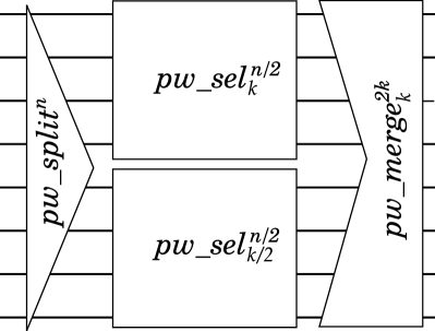
(a) one step

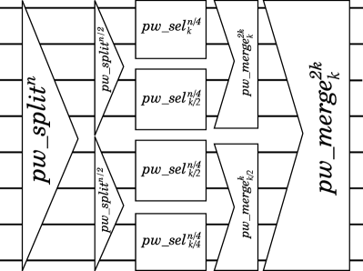
(b) two steps

Figure 4: Pairwise Cardinality Network

Lemma 5.

Let $k\in\mathbb{N}$. Then $2V(pw\_merge^{2k}_{k})+V(pw\_merge^{k}_{k/2})=5k\log k-6k+6$ and $2C(pw\_merge^{2k}_{k})+C(pw\_merge^{k}_{k/2})=\frac{15}{2}k\log k-9k+9$.

Proof.

The number of 2-comparator used is:

$$2|pw\_merge^{2k}_{k}|+|pw\_merge^{k}_{k/2}|=\frac{5}{2}k\log k-3k+3$$

Elementary calculation gives the desired result. ∎

We now count the number of variables and clauses for the 4-Wise Selection Network, again, disregarding the recursive steps.

Lemma 6.

Let $k\in\mathbb{N}$. Then $V(4w\_merge^{4k}_{k})=k\log k+\frac{7}{6}k-5$, $C(4w\_merge^{4k}_{k})=\frac{15}{4}k\log k-\frac{33}{24}k-10$.

Proof.

We separately count the number of 2, 3 and 4-comparators used in the merger (Network 3). By the assumption that $k\leq n/4$ we get $|\bar{w}|=k$, $|\bar{x}|=k/2$, $|\bar{y}|=k/3$, $|\bar{z}|=k/4$ and $h_{1}=k/2$. We will consider iterations 1, 2 and 3 separately and then provide the formulas for the number of comparators for iterations 4 and beyond. Results are summarized in Table 1.

In the first iteration $h_{1}=k/2$, which means that sets of $j$-values in the first two inner loops (lines 7–10 and 11–13) are empty. On the other hand, $1\leq j\leq\min(k_{1}-h_{1},k_{2},h_{1})=k/2$ (line 14), therefore $k/2$ 2-comparators are used. In fact it is true for every iteration $i$ that $\min(k_{1}-h_{i},k_{2},h_{i})=h_{i}=k/2^{i}$. We note this fact in column 3 of Table 1 (the first term of each expression). For the next iterations we only need to consider the first and second inner loops of the algorithm.

In the second iteration $h_{2}=k/4$, therefore in the first inner loop only the condition in line 10 will hold, and only when $j\leq k/3-k/4=k/12$, hence $k/12$ 2-comparators are used. In the second inner loop the $j$-values satisfy condition $1\leq j\leq\min(k_{2}-h_{2},k_{3},h_{2})=k/4$. Therefore the condition in line 12 will hold for each $j\leq k/4$, hence $k/4$ 3-comparators are used. In fact it is true for every iteration $i\geq 2$ that $\min(k_{2}-h_{i},k_{3},h_{i})=k/2^{i}$, so the condition in line 12 will be true for $1\leq j\leq k/2^{i}$. We note this fact in column 4 of Table 1. For the next iterations we only need to consider the first inner loop of the algorithm.

In the third iteration $h_{3}=k/8$, therefore $j$-values in the first inner loop satisfy the condition $1\leq j\leq\min(k_{3}-h_{3},k_{4})=5k/24$ and the condition in line 8 will hold for each $j\leq 5k/24$, hence $5k/24$ 4-comparators are used.

From the forth iteration $h_{i}\leq k/16$, therefore for every $1\leq j\leq\min(k_{3}-h_{i},k_{4})=k/4$ the condition in line 8 holds. Therefore $k/4$ 4-comparators are used.

What’s left is to sum 2,3 and 4-comparators throughout $\log k$ iterations of the algorithm. The results are are presented in Table 1. Elementary calculation gives the desired result.

$i$	$h_{i}$	#2-comparators	#3-comparators	#4-comparators
$1$	$\frac{k}{2}$	$\frac{k}{2}$	$0$	$0$
$2$	$\frac{k}{4}$	$\frac{k}{4}+\frac{k}{12}$	$\frac{k}{4}$	$0$
$3$	$\frac{k}{8}$	$\frac{k}{8}$	$\frac{k}{8}$	$\frac{5k}{24}$
$\geq 4$	$\frac{k}{2^{i}}$	$\frac{k}{2^{i}}$	$\frac{k}{2^{i}}$	$\frac{k}{4}$
	Sum	$\frac{13}{12}k-1$	$\frac{k}{2}-1$	$\frac{1}{4}k\log k-\frac{13k}{24}$

Table 1: Number of comparators used in different iterations of Network 3

∎

Let $V_{PCN}=2V(pw\_merge^{2k}_{k})+V(pw\_merge^{k}_{k/2})$, $C_{PCN}=2C(pw\_merge^{2k}_{k})+C(pw\_merge^{k}_{k/2})$, $V_{4W}=V(4w\_merge^{4k}_{k})$ and $C_{4W}=C(4w\_merge^{4k}_{k})$. Then the following corollary shows that using 4-column pairwise merging networks produces smaller encodings than their 2-column counterpart.

Corollary 2.

Let $k\in\mathbb{N}$ such that $k\geq 4$. Then $V_{4W}<V_{PCN}$ and $C_{4W}<C_{PCN}$.

For the following theorem, note that $V(4w\_split^{n})=V(pw\_split^{n})=n$.

Theorem 5.1.

Let $n,k\in\mathbb{N}$ such that $1\leq k\leq n/4$ and $n$ and $k$ are both powers of 4. Then $V(4w\_sel^{n}_{k})\leq V(pw\_sel^{n}_{k})$.

Proof.

Proof is by induction. For the base case, consider $1=k<n$. It follows that $V(4w\_sel^{n}_{k})=V(pw\_sel^{n}_{k})=V(max^{n})$. For the induction step assume that for each $(n^{\prime},k^{\prime})\prec(n,k)$ (in lexicographical order), where $k\geq 4$, the inequality holds, we get:

$$V(4w\_sel^{n}_{k})=V(4w\_split^{n})+\sum_{1\leq i\leq 4}V(4w\_sel^{n/4}_{k/i})+V(4w\_merge^{4k}_{k})$$

(by the construction of )

(by the induction hypothesis)

(by Corollary 2 and because )

(because )

(by the construction of )

∎

Now we will count how many variables and clauses are needed in order to merge 4 sorted sequences returned by recursive calls of Odd-Even Selection Network and 4-Odd-Even Selection Network, respectively. Two-column selection network using odd-even approach is presented in [9]. We briefly introduce this network with the following three-step recursive procedure (omitting the base case):

1. Split the input $\bar{x}\in\{0,1\}^{n}$ into two sequences $\bar{x}^{1}=\bar{x}_{\textit{odd}}$ and $\bar{x}^{2}=\bar{x}_{\textit{even}}$.

2. Recursively select top $k$ sorted elements from $\bar{x}^{1}$ and top $k$ sorted elements from $\bar{x}^{2}$.

3. Merge the outputs of the previous step using a Odd-Even Merging Network of order $(2k,k)$ and output the top $k$ elements.

If we treat the merging step as a network $oe\_merge^{2k}_{k}$, then the number of 2-comparators used in the Odd-Even Selection Network of order $(n,k)$ can be written as:

$$|2oe\_sel^{n}_{k}|=\left\{\begin{array}[]{l l}2|2oe\_sel^{n/2}_{k}|+|2oe\_merge^{2k}_{k}|&\quad\text{if $k<n$}\\ |oe\_sort^{k}|&\quad\text{if $k=n$}\\ |max^{n}|&\quad\text{if $k=1$}\\ \end{array}\right.$$ (9)

One can check that Step 3 requires $|2oe\_merge^{2k}_{k}|=k\log k+1$ 2-comparators. Overall number of 2-comparators was already calculated in [9].

Lemma 7 ([9]).

For $k\leq n$ (both powers of two) $2oe\_sel^{n}_{k}$ uses $\frac{1}{4}n\log^{2}k+\frac{3}{4}n\log k-k\log k$ 2-comparators.

The schema of this network is presented in Figure 5. Similarly to the previous case, in order to count the number of comparators used in merging 4 sorted sequences we need to expand the recursive step by one level (see Figure 5b).

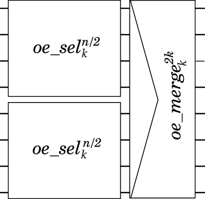
(a) one step

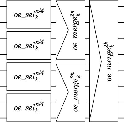
(b) two steps

Figure 5: Pairwise Cardinality Network

Lemma 8.

$3V(2oe\_merge^{2k}_{k})=6k\log k+6$, $3C(2oe\_merge^{2k}_{k})=9k\log k+9$.

Proof.

The number of 2-comparator used is:

$$3|2oe\_merge^{2k}_{k}|=3k\log k+3$$

Elementary calculation gives the desired result. ∎

Now we do the same counting for our 4-Odd-Even Selection Network based on Networks 2 and 5.

Lemma 9.

Let $k\in\mathbb{N}$. Then $V(4oe\_merge^{4k}_{k})\leq 2k\log k+16k-4\log k-6$ and $C(4oe\_merge^{4k}_{k})\leq 3k\log k+33k-6\log k-9$.

Proof.

We separately count the number of 2 and 4-comparators used. We count the comparators in the merger (Network 5). By the assumption that $k\leq n/4$ and that $k$ is the power of 4 we get that $|\bar{w}|=|\bar{x}|=|\bar{y}|=|\bar{z}|=k$. This implies that $s=4k$ and $sa=sb=2k$.

In the algorithm 4-comparators are only used in the base case (line 3–5). Furthermore number of 4-comparators is only dependent on the variable $s$. The solution to the following recurrence gives the sought number: $\{A(4)=1;A(s)=2A(s/2),\text{for }s>4\}$, which is equal to $s/4=k$.

We now count the number of 2-comparators used. The combine operations in lines 9–11 uses $(2k/2+1+k)/2\leq k+1$ 2-comparators. The total number of 2-comparators is then a solution to the following recurrence:

$$B(s,k)=\begin{cases}0&\quad\text{if }s\leq 4\\ B(s/2,k/2+2)+B(s/2,k/2)+k+1&\quad\text{otherwise }\\ \end{cases}$$

We claim that $B(s,k)\leq k\log\frac{s}{2}-k-2\log s+\frac{3}{2}s+1$. This can be easily verified using induction. Applying $s=4k$ gives us the upper bound on number of 2-comparators used, which is $k\log k+6k-2\log k-3$.

Elementary calculation gives the desired result. ∎

Let $V_{2OE}=3V(oe\_merge^{2k}_{k})$, $C_{2OE}=3C(oe\_merge^{2k}_{k})$, $V_{4OE}=V(4oe\_merge^{4k}_{k})$ and $C_{4OE}=C(4oe\_merge^{4k}_{k})$.

Corollary 3.

Let $k\in\mathbb{N}$. If $k\geq 16$, then $V_{4OE}\leq V_{2OE}$. If $k\geq 64$, then $C_{4OE}\leq C_{2OE}$

The corollary above does not cover all values of $k$. For the sake of the next theorem we set $k=4$ and compare values $V(4oe\_sel^{n}_{4})$ and $V(2oe\_sel^{n}_{4})$ in the following lemma. We do similar calculations for $C(4oe\_sel^{n}_{k})$ and $C(2oe\_sel^{n}_{k})$, for $k\in\{4,16\}$.

Lemma 10.

Let $n\in\mathbb{N}$ such that $n\geq 16$ and $n$ is a power of 4. Then $V(4oe\_sel^{n}_{4})\leq V(2oe\_sel^{n}_{4})$.

Proof.

Applying $k=4$ to the formula in Lemma 7 gives $\frac{5}{2}n-8$ 2-comparators and therefore $V(2oe\_sel^{n}_{4})=5n-16$.

On the other hand, we calculate the value $B(s,k)$ from Lemma 9 more accurately when $k=4$ to get accurate result for $V(4oe\_merge^{s}_{4})$ and, in consequence, for $V(4oe\_sel^{n}_{4})$. First we rewrite the formula so it represents the number of variables used in $4oe\_merge^{n}_{k}$:

$$B^{*}(s,k)=\begin{cases}4&\quad\text{if }s\leq 4\\ B^{*}(s/2,\left\lfloor k/2\right\rfloor+2)+B^{*}(s/2,\left\lfloor k/2\right\rfloor)+4\left\lfloor k/2\right\rfloor+2&\quad\text{otherwise }\\ \end{cases}$$

The change is straightforward. Since $s=4k$, we can calculate by hand that $B^{*}(16,4)=42$. The sought value is given by:

$$V(4oe\_sel^{n}_{4})=\begin{cases}V(4oe\_merge^{16}_{4})+16&\quad\text{if }n=16\\ 4V(4oe\_sel^{n/4}_{4})+V(4oe\_merge^{16}_{4})&\quad\text{otherwise }\\ \end{cases}$$

In the first case we use one merger of order $(16,4)$ and 4 4-comparators. The second case is straightforward. Since $V(4oe\_merge^{16}_{4})=B^{*}(16,4)$, so the recursive formula above can be reduced into:

$$f(n)=\begin{cases}58&\quad\text{if }n=16\\ 4f(n/4)+42&\quad\text{otherwise }\\ \end{cases}$$

for which the solution is $f(n)=\frac{9}{2}n-14$. Obviously $\frac{9}{2}n-14\leq 5n-16$, for $n\geq 4$, so we are done. ∎

Theorem 5.2.

Let $n,k\in\mathbb{N}$ such that $1\leq k\leq n/4$ and $n$ and $k$ are both powers of 4. Then $V(4oe\_sel^{n}_{k})\leq V(2oe\_sel^{n}_{k})$.

Proof.

Proof is by induction. For the base case, consider $1=k<n$. It follows that $V(2oe\_sel^{n}_{k})=V(4oe\_sel^{n}_{k})=V(max^{n})$. The case $n>k=4$ is handled by Lemma 10. For the induction step assume that for each $(n^{\prime},k^{\prime})\prec(n,k)$ (in lexicographical order), where $k\geq 16$, the inequality holds, we get:

$$V(4oe\_sel^{n}_{k})=4V(4oe\_sel^{n/4}_{k})+V(4oe\_merge^{4k}_{k})$$

(by the construction of )

(by the induction hypothesis)

(by Corollary 3)

(by the construction of )

∎

6 Experimental Evaluation

As it was observed in [1], having a smaller encoding in terms of number of variables or clauses is not always beneficial in practice, as it should also be accompanied with a reduction of SAT-solver runtime. In this section we assess how our encodings based on the new family of selection networks affect the performance of a SAT-solver.

Our algorithms that encode CNF instances with cardinality constraints into CNFs were implemented as an extension of MiniCard ver. 1.1, created by Mark Liffiton and Jordyn Maglalang. MiniCard uses three types of solvers:

• minicard - the core MiniCard solver with native AtMost constraints,

• minicard_encodings - a cardinality solver using CNF encodings for AtMost constraints,

• minicard_simp_encodings - the above solver with simplification / preprocessing.

The main program in minicard_encodings has an option to generate a CNF formula, given a CNFP instance (CNF with the set of cardinality constraints) and to select a type of encoding applied to cardinality constraints. Program run with this option outputs a CNF instance that consists of collection of the original clauses with the conjunction of CNFs generated by given method for each cardinality constraint. No additional preprocessing and/or simplifications are made. Authors of minicard_encodings have implemented six methods to encode cardinality constraints and arranged them in one library called Encodings.h. Our modification of MiniCard is that we added implementations of encodings presented in this paper and put them in the library Encodings_MW.h. Then, for each CNFP instance and each encoding method, we used MiniCard to generate CNF instances. After preparing, the benchmarks were run on a different SAT-solvers. Our extension of MiniCard, which we call KP-MiniCard, is available online.

We use two SAT-solvers in this evaluation. The first one is the well known MiniSat (ver. 2.2.0) created by Niklas Eén and Niklas Sörensson. The second SAT-solver is the GlueMiniSat (ver. 2.2.8), by Hidetomo Nabeshima, Koji Iwanuma and Katsumi Inoue. All experiments were carried out on the machines with Intel(R) Core(TM) i7-2600 CPU @ 3.40GHz.

Detailed results are available online. We publish spreadsheets showing running time for each instance, speed-up/slow-down tables for our encodings, number of time-outs met and total running time.

Encodings: From this paper we choose two multi-column selection networks for evaluation:

• 4WISE - 4-column selection network based on pairwise approach (Networks 1 and 3),

• 4OE - 4-column odd-even selection network based on Networks 2 and 5.

We compare our encodings to some others found in the literature. We consider the Pairwise Cardinality Networks [9] to rival our 4-column pairwise selection network. We also consider a solver called MiniSat+ which implements techniques to encode Pseudo-Boolean constraints to propositional formulas [10]. Since cardinality constraints are a subclass of Pseudo-Boolean constraints, we can measure how well the encodings used in MiniSat+ perform, compared with our methods. The solver chooses between three techniques to generate SAT encodings for Pseudo-Boolean constraints. These convert the constraint to: a BDD structure, a network of binary adders, a network of sorters. The network of adders is the most concise encoding, but it has poor propagation properties and often leads to longer computations than the BDD based encoding. The network of sorters is the implementation of classic odd-even (2-column) sorting network by Batcher [6]. Calling the solver we can choose the encoding with one of the parameters: -ca, -cb, -cs. By default, MiniSat+ uses the so called Mixed strategy, where program chooses which method (-ca, -cb or -cs) to use in the encodings, and this depends on size of the input and memory restrictions. We don’t include Mixed strategy in the results, as the evaluation showed that it performs almost the same as -cb option. The generated CNFs were written to files with the option -cnf=$<$file$>$.

To sum up, here are the competitors’ encodings used in this evaluation:

• PCN - the Pairwise Cardinality Networks (our implementation)

• CA - encodings based on Binary Adders (from MiniSat+)

• CB - encodings based on Binary Decision Diagrams (from MiniSat+)

• CS - the Odd-Even Sorting Networks (from MiniSat+)

Additionally, encodings 4WISE, 4OE and PCN were extended, following the idea presented in [1], where authors use Direct Cardinality Networks in their encodings for sufficiently small values of $n$ and $k$. Values of $n$ and $k$ for which we substitute the recursive calls with Direct Cardinality Network were selected based on our knowledge and some experiments.

Solver MiniSat+ have been slightly modified, namely, we fixed several bugs such as the one reported in the experiments section of [5].

Benchmarks: We used the following sets of benchmarks:

1. MSU4 suite: A set consisting of about 14000 benchmarks, each of which contains a mix of CNF formula and multiple cardinality constraints. This suite was created from a set of MaxSAT instances reduced from real-life problems, and then it was converted by the implementation of msu4 algorithm [14]. This algorithm reduces a MaxSAT problem to a series of SAT problems with cardinality constraints. The MaxSAT instances were taken from the Partial Max-SAT division of the Third Max-SAT evaluation. We perform experiments for this benchmarks using MiniSat.

2. PB15 suite: A set of benchmarks from the Pseudo-Boolean Evaluation 2015. One of the categories of the competition was DEC-LIN-32-CARD, which contains 2289 instances – we use these in our evaluation. Every instance is a set of cardinality constraints. This set of benchmarks were evaluated using GlueMiniSat.

	4OE speed-up						4OE slow-down
	TO	4.0	2.0	1.5	1.1	Total	TO	4.0	2.0	1.5	1.1	Total
PCN	54	73	1	6	9	143	1	6	0	2	4	13
4WISE	26	48	11	5	4	94	2	7	4	3	4	20
CA	840	1114	0	6	4	1964	2	3	1	1	3	10
CB	100	187	0	7	3	297	3	6	1	4	2	16
CS	53	73	0	2	4	132	2	17	0	2	0	21
	4WISE speed-up						4WISE slow-down
	TO	4.0	2.0	1.5	1.1	Total	TO	4.0	2.0	1.5	1.1	Total
PCN	30	35	16	8	12	101	1	7	6	2	6	22
4OE	2	7	4	3	4	20	26	48	11	5	4	94
CA	816	1083	13	7	8	1927	2	3	4	1	3	13
CB	86	154	23	11	6	280	13	18	5	2	4	42
CS	35	50	6	2	5	98	8	34	5	3	3	53

Table 2: Comparison of encodings in terms of SAT-solver runtime on MSU suite. We count number of benchmarks for which 4OE and 4WISE showed speed-up or slow-down factor with respect to different encodings.

	4OE speed-up						4OE slow-down
	TO	4.0	2.0	1.5	1.1	Total	TO	4.0	2.0	1.5	1.1	Total
PCN	4	4	1	4	11	24	0	0	2	4	8	14
4WISE	2	0	2	4	9	17	0	0	3	3	10	16
CA	10	13	32	13	20	88	2	2	6	5	15	30
CB	8	5	15	7	18	53	6	0	5	14	7	32
CS	15	10	17	14	19	75	6	1	5	8	17	37

Table 3: Comparison of encodings in terms of SAT-solver runtime on PB15 suite. We count number of benchmarks for which 4OE showed speed-up or slow-down factor with respect to different encodings.

		4OE	4WISE	CS	PCN	CB	CA
MSU4	Total time	25319	44978	52284	62695	102894	695003
	Time-outs	16	40	67	69	113	854
PB15	Total time	2291394	2292065	2311042	2294726	2301762	2312199
	Time-outs	1240	1242	1249	1244	1242	1248

Table 4: Total running time (in seconds) of all instances and total number of time-outs.

Results: The time-out limit in the SAT-solvers was set to 600 seconds in case of MSU4 suite, and 1800 seconds for PB15 suite. When comparing two encodings we only considered instances for which at least one achieved the SAT-solver runtime of at least 10% of the time-out limit. All other instances were considered trivial, and therefore were not included in the results. We also filtered out the instances for which relative percentage deviation of the running time of encoding A w.r.t the running time of encoding B was less than 10% (and vice-versa), i.e., $|(t(A,I)-t(B,I))|/\min(t(A,I),t(B,I))\leq 0.1$, where $t(E,I)$ is the time in which the SAT-solver terminated given a CNF generated from the instance $I$ using encoding $E$.

Tables 2 and 3 present speed-up and slow-down factors for encodings 4OE and 4WISE w.r.t all other encodings. For PB15 suite we only show speed-up/slow-down of 4OE, since from the first batch of tests (on MSU4 suite) we can conclude that it is the superior encoding. Explanation of how to read the tables now follows. Consider the comparison of encoding A w.r.t encoding B. In the speed-up section, TO indicates the number of instances run with encoding B that ended as time-outs but were solved while run with encoding A. The TO value in the slow-down section means that the opposite is true. Column headers with numbers indicate speed-up (slow-down) factors for the encoding A, for example, instances counted in column $1.5$ are those for which $2.0\cdot t(A,I)\geq t(B,I)>1.5\cdot t(A,I)$ for speed-up, and $2.0\cdot t(A,I)\leq t(B,I)<1.5\cdot t(A,I)$ for slow-down. In case of factor $4.0$ the other coefficient is $\infty$.

From the evaluation we can conclude that the best performing encoding is 4OE, on both MSU4 and PB15 suites. On MSU4 suite (Table 2), the superiority is apparent, as our encoding achieve significant speed-up factor w.r.t all other encodings. The runner-up encoding is 4WISE, which performs worse than 4OE, but still beats all other encodings. This is also reflected in the total running times and number of time-outs met over all instances – those values are presented in Table 4. We see that on MSU4 suite, SAT-solver finished twice as fast using encoding 4OE rather than CS, and solved almost all instances in given time. Similar observation can be made for 4WISE w.r.t PCN, where our encoding has about 18 000 seconds (5 hours) smaller total time and 75% less time-outs. This shows that using 4-column selection networks is more desirable than using 2-column selection/sorting networks for encoding cardinality constraints. Encodings CA and CB had the worst performance on MSU4 suite.

As for the results on PB15 suite, we see that the total running times and time-outs are similar (Table 4) for all encodings. This is due to the fact that PB15 suite contains a lot of hard instances and a lot of trivial instances, so the true competition boils down to a few medium-sized instances. Still, encoding 4OE is the clear winner, having finished computations about 20 000 seconds (5.5 hours) faster than CS. Encoding 4WISE performs similar to 4OE, with only about 10 minutes gap in the total running time, but it is the latter that solved the most number of instances. Encoding 4OE also outperforms all other encodings in terms of speed-up, which is presented in Table 3.

In Figure 6 we present two cactus plots, where x-axis gives the number of solved instances and the y-axis the time needed to solve them (in seconds) using given encoding. Results for MSU4 suite are in Figure 6a and for PB15 suite in Figure 6b. Notice that we did not include the CA encoding in the first plot, as it was not competitive to the other encodings. From the plots we can see again that the 4OE encoding outperforms all other encodings.

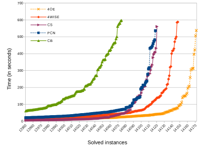
(a) MSU4

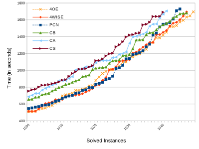
(b) PB15

Figure 6: Number of solved instances of MSU4 suite and PB15 suite in given time.

7 Conclusions

In this paper we presented a family of multicolumn selection networks based on odd-even and pairwise approach, that can be used to encode cardinality constraints. We showed detailed constructions where the number of columns is equal to 4 and showed that their CNF encodings are smaller than their 2-column counterparts. We extended the encodings by applying the Direct Cardinality Networks of [1] for sufficiently small input. The new encodings were compared with the selected state-of-art encodings based on comparator networks, adders and binary decision diagrams. The experimental evaluation shows that the new encodings yield significant speed-ups in the SAT-solver performance.

Developing new methods to encode cardinality constraints based on comparator networks is important from the practical point of view. Using such encodings give an extra edge in solving optimization problems for which we need to solve a series of problems that differ only in that a bound on cardinality constraint $x_{1}+\dots+x_{n}\leq k$ becomes tighter, i.e., by decreasing $k$ to $k^{\prime}$. In this setting we only need to add one more clause $\neg y_{k^{\prime}}$, and the computation can be resumed while keeping all the previous clauses untouched. This operation is allowed because if a comparator network is a $k$-selection network, then it is also a $k^{\prime}$-selection network, for any $k^{\prime}<k$. This property is called incremental strengthening and most state-of-art SAT-solvers provide an interface for doing this.

References

- [1] Abío, I., Nieuwenhuis, R., Oliveras, A., Rodríguez-Carbonell, E.: A Parametric Approach for Smaller and Better Encodings of Cardinality Constraints. In: C. Schulte, (ed), Principles and Practice of Constraint Programming - CP 2013, LNCS, vol. 8124, pp. 80–96. Springer Heidelberg, (2013).
- [2] Anbulagan, Grastein, A.: Importance of Variables Semantic in CNF Encoding of Cardinality Constraints. In: V. Bulitko and J. C. Beck, (ed), Eighth Symposium on Abstraction, Reformulation, and Approximation, SARA’09. AAAI, 2009.
- [3] Asín, R., Nieuwenhuis, R., Oliveras, A., Rodríguez-Carbonell, E.: Cardinality networks: a theoretical and empirical study. Constraints, 16(2):195–221, (2011).
- [4] Asín, R., Nieuwenhuis, R.: Curriculum-based course timetabling with SAT and MaxSAT. Annals of Operations Research, 218(1):71–91, (2014).
- [5] Aavani, A., Mitchell, D.G., Ternovska, E.: New encoding for translating pseudo-Boolean constraints into SAT. In: Frisch, A.M., Gregory, P. (eds.) SARA, AAAI (2013).
- [6] K. E. Batcher.: Sorting networks and their applications. In: Proc. of the April 30–May 2, 1968, Spring Joint Computer Conference, AFIPS ’68 (Spring), pp. 307–314, ACM, New York, NY, USA, (1968).
- [7] K. E. Batcher, Lee, D.: A Multiway Merge Sorting Network. In: IEEE Transactions on Parallel and Distributed Systems, Vol. 6, No. 2, February 1995, pp. 211–215.
- [8] Biere, A., Cimatti, A., Clarke, E., Zhu, Y.: Symbolic Model Checking without BDDs. In: Proc. of 5th International Conference on Tools and Algorithms for the Construction and Analysis of Systems (TACAS’99), LNCS vol. 1579, pp. 193–207, Springer Heidelberg (1999).
- [9] Codish, M., Zazon-Ivry, M.: Pairwise cardinality networks. In: E. Clarke and A. Voronkov, (eds), Logic for Programming, Artificial Intelligence, and Reasoning, LNCS vol. 6355, pp. 154–172. Springer Heidelberg (2010).
- [10] Eén, N., Sörensson, N.: Translating pseudo-boolean constraints into sat. Journal on Satisfiability, Boolean Modeling and Computation, 2:1–26, (2006).
- [11] Gao, Q., Liu, Z., Zhao, L.: An efficient multiway merging algorithm. Science in China Series E: Technological Sciences, vol. 41:5, October 1998, Science in China Press, 1998.
- [12] Karpiński, M., Piotrów, M.: Smaller Selection Networks for Cardinality Constraints Encoding. In: G. Pesant, (ed), Principles and Practice of Constraint Programming - CP 2015, LNCS, vol. 9255, pp. 210-225. Springer International Publishing, 2015.
- [13] Knuth, D. E.: The Art of Computer Programming, Volume 3: (2Nd Ed.) Sorting and Searching. Addison Wesley Longman Publishing Co., Inc., Redwood City, CA, USA, (1998).
- [14] Marques-Silva, J., Planes, J.: Algorithms for Maximum Satisfiability using Unsatisfiable Cores. In: 2008 Conference on Design, Automation and Test in Europe Conference, DATE’08, pp. 408–413. IEEE Computer Society, 2008.
- [15] Parberry, I.: The pairwise sorting network. Parallel Processing Letters, 2:205–211, (1992).
- [16] Schutt, A., Feydy, T., Stuckey, P., Wallace, M.: Why cumulative decomposition is not as bad as it sounds. In: I. Gent, (ed), Principles and Practice of Constraint Programming - CP 2009, LNCS, vol. 5732, pp. 746–761. Springer Heidelberg, (2009).