New higher-order transition in causal dynamical triangulations
Abstract
We reinvestigate the recently discovered bifurcation phase transition in Causal Dynamical Triangulations (CDT) and provide further evidence that it is a higher order transition. We also investigate the impact of introducing matter in the form of massless scalar fields to CDT. We discuss the impact of scalar fields on the measured spatial volumes and fluctuation profiles in addition to analysing how the scalar fields influence the position of the bifurcation transition.
PACS numbers: 04.60.Gw, 04.60.Nc
1 Introduction
The reasons for attempting to quantize gravity are manifold, including the fact that every other fundamental force can be understood within the framework of quantum field theory. However, treating gravity as a perturbative quantum field theory results in a complete loss of predictive power, since in order to define such a theory one would first need to experimentally determine an infinite number of independent coefficients. The divergent number of counterterm coefficients associated with the perturbative treatment of general relativity have been confirmed by explicit calculation, appearing at two-loops for pure gravity [1] and at one-loop for gravity including matter [2]. The divergences associated with the perturbative treatment of gravity has generated considerable interest in nonperturbative formulations, one of the most promising of which is the so-called asymptotic safety scenario.
First proposed by Weinberg [3], asymptotic safety posits the existence of an ultra-violet fixed point (UVFP) under the flow of the renormalization group of gravitational couplings. If there exist only a finite number of such couplings that are attracted to the fixed point at high energies, then asymptotic safety may define a finite and predictive theory of quantum gravity in the nonperturbative regime. There is mounting evidence for the existence of an UVFP, ranging from the -expansion of spacetime dimensionality [4] to functional renormalization group results [5, 6, 7]. A lattice formulation of quantum gravity provides a complimentary approach to asymptotic safety, since it permits the definition of a gravitational path integral that can be studied in the nonperturbative regime. Lattice gravity can also provide direct evidence for asymptotic safety, since in a lattice formulation an UVFP would appear as a higher (than first) order critical point, the approach to which would define a continuum limit.
One of the first lattice regularizations of quantum gravity is Euclidean dynamical triangulations (EDT), which attempts to define a nonperturbative theory of quantum gravity as the continuum limit of a sum over discrete spacetime geometries. In this approach spacetime is approximated by a network of locally flat -dimensional triangles that are connected via their -dimensional faces. Unfortunately, early EDT simulations found just two phases, neither of which resembled -dimensional semiclassical general relativity.111Although there are some encouraging signs that a particular modification of EDT may have a suitable infra-red limit after a certain fine-tuning is implemented [8]. Moreover, it was shown that these two phases are separated by a first order phase transition, making the existence of a continuum limit improbable. Motivated by the difficulties encountered in the original EDT formulation, a causality condition was added to the model whereby the lattice is foliated into space-like hypersurfaces of fixed topology, an approach known as causal dynamical triangulations (CDT) [9]. The inclusion of this additional constraint appears to cure the problems found in the original EDT formulation.
The path integral for pure CDT quantum gravity is defined by
| (1) |
where one performs a sum over all discrete triangulations allowed by the causality constraint. is a symmetry factor encoding the number of equivalent ways of labelling the vertices in , and is the discretised Einstein-Hilbert action of the triangulation [10], where
| (2) |
denotes the number of simplicial building blocks with vertices on hypersurface and vertices on hypersurface . The number of vertices in the triangulation is given by . The CDT action includes three bare coupling constants , and . is inversely proportional to Newton’s constant, is related to the ratio of the length of space-like and time-like links on the lattice and is proportional to the cosmological constant. is tuned to a (pseudo)-critical value in the simulations such that one can take an infinite-volume limit. The parameter space of CDT can then be explored by varying and .
Using Monte Carlo simulations the CDT parameter space spanned by and has now largely been mapped out, as shown schematically in Fig. 1. To date there are 4 known phases of CDT, labelled A, B, and . Phases and do not appear to reproduce general relativity in the semiclassical limit, and are generally regarded as lattice artifacts. The recently discovered bifurcation phase also has a number of unphysical features [11] such as a very large, and possibly infinite, effective spacetime dimension [12]. However, the de Sitter phase has a volume profile that closely matches Euclidean de Sitter space [13] and an effective dimension consistent with [14, 15, 16], thus defining the physically interesting phase of CDT.
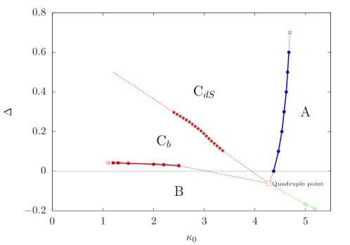
The transition is known to be first order, while the - transition is likely second order [17]. The order of the transition has yet to be definitively determined, although preliminary calculations suggest a higher-order transition [18]. Conclusively determining the order of the transition may prove an important result in CDT, since a second order transition would raise the possibility of defining a continuum limit from within the physically interesting de Sitter phase . In this work we aim to more definitively determine the order of the transition.
Another question that this work addresses is how the inclusion of matter fields affects the phase structure of CDT. In particular, it is possible that the bifurcation phase is an artifact of the naive pure gravity formulation of CDT, and that the inclusion of a sufficient number of matter fields may be a necessary condition for the universe to exhibit the correct semiclassical behaviour, as suggested in Ref. [19]. In this work we investigate this possibility by coupling CDT to massless scalar fields and examining how this affects the extent of the bifurcation phase.
This paper is organised as follows. In section 2 we define the order parameter used to study the phase transition and detail how a finite-size scaling analysis can be used to indicate the order of this transition. After reviewing some technical details in section 3 regarding the numerical implementation of adding massless scalar fields to CDT, we study how the inclusion of such matter fields affects the position of the transition in the parameter space. A discussion and summary of the results obtained in this work are presented in section 4.
2 The order of the transition
Phase transitions are often associated with a breaking of some symmetry. To quantify the transition one can define an order parameter that captures the symmetry difference between the phases. Such an order parameter is typically zero (or constant) inside the symmetric phase and non-zero (or non-constant) in the symmetry broken phase. The first order phase transition point is then characterised by a discontinuity in the first order derivative of the in the infinite volume limit, whereas for a th order transition the th order derivatives are continuous but the th order derivative is not.
In numerical simulations it is quite difficult to distinguish the order of a phase transition by just looking at the (dis)continuity of some order parameter’s th derivative. The reason is twofold. First, numerical simulations are always performed with finite precision and it is very difficult to judge whether a sudden jump in some order parameter (or its derivative) is caused by a real discontinuity, or is actually caused by insufficient measurement precision. Secondly, numerical simulations always require finite systems (volumes) and thus no real phase transitions take place (all infinities are replaced by large but finite numbers dependent on the system’s size). One should therefore carefully analyse finite size effects and extrapolate the results to the infinite volume limit.
As an example, one can locate (pseudo-)critical points by searching the parameter space for peaks in the susceptibility of the order parameter
| (3) |
Positions of such transition points in the parameter space will typically depend on the system volume and by measuring how they change with increasing volume one can in principle determine the position of the true phase transition in the infinite volume limit by extrapolation. One can also use the same method to determine critical exponents, whose values may indicate the order of the phase transition.
The results presented in this section are a continuation of work initiated in Refs. [20, 18], where a suitable choice of order parameters was suggested based on microscopic geometric properties of the bifurcation phase . Distribution of volume in phase is markedly different than in the de Sitter phase , with spatial volume concentrated in clusters connected by vertices of very high coordination number [20, 11]. This geometric difference is presumably caused by a breaking of homogeneity222The homogeneity of phase should be understood in a statistical sense, i.e. the emergent average semiclassical background geometry is homogeneous but individual trajectories of the path integral (triangulations) are not. This is in analogy with the ordinary path integral of quantum mechanics where the classical (average) trajectory is smooth but individual path integral trajectories are nowhere differentiable. This homogeneity is not the case in phase where the average geometry is not homogeneous and also individual triangulations are much less homogeneous than inside phase . This is due to the formation of large volume clusters around vertices of very high coordination number present every second lattice time coordinate in phase (see Fig. 3, right, and Fig. 3). Such volume clusters constitute most of the individual triangulations of phase and they overlap forming a four-dimensional structure. Geometry inside the structure is markedly different than the geometry outside since neither the average space-time geometry nor average spatial geometries are homogeneous. In phase some volume clusters also form around the highest order vertices due to quantum fluctuations, however in this case the volume clusters are much smaller and their overlap is only statistical. As a result there is no distinct four-dimensional structure and the average space-time and spatial geometries seem to be homogeneous. The differences between the geometry of phases and will be discussed in detail in forthcoming articles. of phase and it can be exploited to signal the transition to phase .
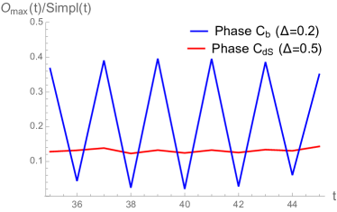
When one looks inside the de Sitter phase and measures the distribution of vertex coordination numbers444Vertex coordination number is defined as a number of 4-simplices sharing a given vertex. (see Fig. 3 left) one observes that there is no clear gap between the highest order vertex (the one with maximal coordination number in a given time slice ) and other vertices present in the same slice . This is independent on the parity of the lattice time coordinate . The situation changes when one goes inside the bifurcation phase . Here the distribution of vertex coordination numbers (see Fig. 3 right) depends on . For (say) even the distribution is quite similar to the one observed in phase whereas for odd one observes a clear gap between the highest order vertex and other vertices . The gap rises when one goes deeper and deeper into the bifurcation phase and also when one increases the total lattice volume . As a result the maximal coordination number jumps between odd and even spatial slices in the bifurcation phase , and there is no such jumping in phase (see Fig. 3). In Refs. [20, 18] a simple order parameter based on the above observation was proposed
| (4) |
where is chosen in such a way that is the highest coordination number in a triangulation, i.e. the highest among all high order vertices :
| (5) |
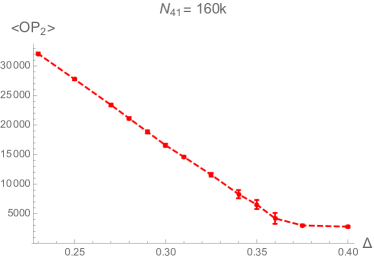
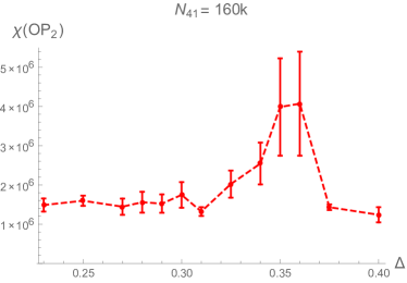
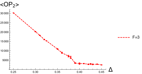
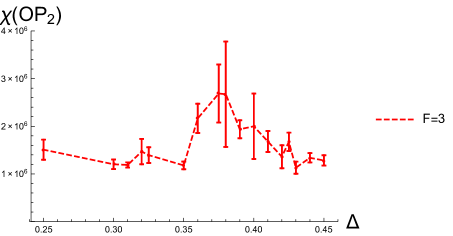
The order parameter is approximately zero in the (more) symmetric phase and non-zero in the symmetry-broken phase . If, for example, one starts from some chosen point in the phase diagram inside phase and lowers one encounters the phase transition to phase when the order parameter starts to rise approximately linearly with decreasing (see Fig. 4 left). The (pseudo-)critical point is signalled by a peak in susceptibility (Fig. 4 right) and, as already explained, its position depends on the lattice volume . One can fit the measured volume dependence to the formula
| (6) |
and compute the critical exponent . A first order transition should be associated with , and accordingly signals a higher order transition. In Fig. 5 we present results obtained for a wider choice of lattice volumes and also much longer Monte Carlo runs than in reference [18]. The critical exponent fitted using formula (6) is which is greater than with a confidence interval of . This result strongly supports the conjecture that the phase transition is a higher order transition. For comparison we also present in Fig. 5 a fit with forced value of critical exponent which seems to be much less likely.

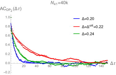
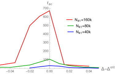
A practical problem with using formula (6), and the reason why we present the updated data, is that one should have transition points measured for a wide choice of lattice volumes, which is very computationally expensive. This is due to the fact that when performing numerical simulations near phase transitions of higher order one usually encounters a so-called critical slowing down, related to very large auto-correlation times of the measured data. The auto-correlation time (in Monte Carlo time) peaks at the phase transition causing the numerical algorithm to loose efficiency, and consequently a very long simulation time is needed to get reliable data in the vicinity of the transition point. This kind of critical slowdown is clearly observed for the phase transition - see Fig 6 (left) where the measured auto-correlation of the order parameter
| (7) |
is shown as a function of the Monte Carlo time difference . Red data points present auto-correlation at the phase transition while other colours are auto-correlations observed slightly away from the phase transition point. One clearly sees that auto-correlation is much longer in the vicinity of the phase transition. This difference can be also exploited to signal the position of (pseudo-)critical points. Fig. 6 (right) presents the auto-correlation time around phase transition points measured for various lattice volumes. The transition points are defined by peaks in susceptibility (3) and the auto-correlation time is obtained by fitting
| (8) |
to the empirical auto-correlation data (7). One clearly sees that the peaks in auto-correlation time are consistent with the peaks in susceptibility. As a side effect the very long auto-correlation time at the phase transition means that a much longer simulation time555Monte Carlo simulations needed to produce susceptibility plots with reasonable error bars and as a consequence to produce Fig. 5 lasted almost one year. is needed to decrease the error bars666Measurement errors were estimated using a single-elimination (binned) jackknife procedure, after blocking the data to account for auto-correlation errors. The procedure was described in detail in Ref. [18]. of the measured observables in the vicinity of the phase transition points. This explains the relatively large error bars observed for the transition points, e.g. in Fig. 4.
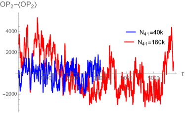
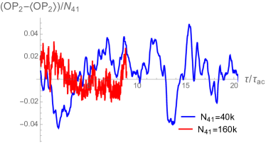
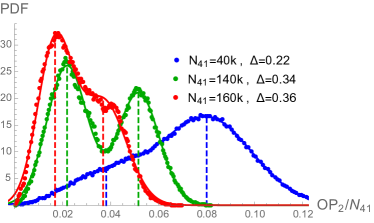
Last but not least, we comment on the double peaks observed in the order parameter histograms (see Fig 8 left) measured at the phase transition points () as already reported in Ref. [18]. The double peaks are caused by the order parameter jumping (in Monte Carlo time) between two values (see Fig. 7) and it was noticed that the frequency of such jumps decreases with increasing lattice volume (see Fig. 7 left), which might in principle signal a first order transition. Now we attribute the decrease in jumping frequency or, in other words, an increase in jumping period to the auto-correlation time which also increases with increasing lattice volume. If one, for example, introduces a dimensionless simulation time by rescaling to account for the auto-correlation difference observed for various lattice volumes one can see that the jumps are less frequent for smaller lattice volumes than they are for larger lattice volumes (see Fig. 7 right). One can also argue that one should look at the normalised order parameters to account for volume difference. Vertex coordination number scales approximately linearly with the number of simplices in a triangulation and thus one should look at rather than . Consequently the amplitude of the (normalised) order parameter jumps seems to decrease with increasing lattice volume. It is clearly visible if one fits a double Gaussian function to the measured histograms of (see Fig. Fig. 8 left). One observes that the Gaussians are only slightly separated. In Fig. 8 (right) we plot the separation of the two peaks as a function of lattice volume . The separation seems to decrease with increasing lattice volume but we have not yet reached a point at which it shrinks to zero. This analysis suggests that the spurious behaviour of which mimics some features of a first order transition is most likely due to finite size effects, and it supports the conjecture that the phase transition is really a higher order transition. Similar phenomena were previously observed for the transition between the bifurcation phase and phase (formerly called the transition), which was shown to be a higher order transition [17], and it was recently explained by a very nontrivial shape of free energy in the vicinity of the phase transition line [11].
3 Adding massless scalar fields to CDT
Motivated by the suggestion of Hartle and Hawking that a sufficient number of matter fields may be a necessary condition to produce the correct classical behaviour of the universe [19] we investigate the effect of adding massless scalar fields to the bare lattice action of CDT. We discuss the impact of the scalar fields on average spatial volume profiles and spatial volume fluctuations in the de Sitter phase and the bifurcation phase . We also analyse whether the position of the transition line is dependent on the number of massless scalar fields .
To this end, we employ a bare action of the form , where is a bare CDT action for pure gravity (2) and is the action for copies of minimally coupled scalar fields ,
| (9) |
with a measure
| (10) |
In (9) we assume that the (real valued) scalar fields are located in simplex centres, and we express the scalar field action in terms of the dual lattice. Consequently, the sums and are over all 4-simplices and over all neighbouring pairs of simplices, respectively. In this work we are only interested in massless scalar fields and so we set the mass parameter equal to zero.
In order to generate configurations, which now consist of a triangulation and superimposed scalar fields, according to action (9), we modify the Metropolis algorithm used thus far. The heat bath method is applied to update the values of the scalar fields. Incorporating the scalar fields does not change the geometrical structure of the Monte Carlo moves, but it influences their weight so that the detailed balance condition is fulfilled [21]. Due to the quadratic form of the scalar field action (9), the heat bath method reduces to generating the updated values of the scalar fields inside the region in which the moves are implemented, i.e. simplices affected by a given move, from a multivariate Gaussian distribution whose parameters depend on the surrounding field values. The scalar fields are updated regardless of whether the move is accepted or not. Such a method is very efficient as the field values inside the region in which the moves are implemented are always altered and the acceptance rate is not impaired. The factors which are not covered by the Gaussian distribution depend only on the field values around the move region and contribute to the weight of the move. The normalisation factors (matrix determinants) can be absorbed by bare coupling redefinitions.
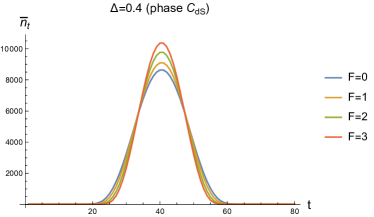
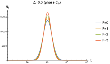
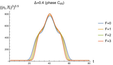
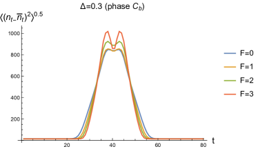
A question that arises is how do the scalar fields impact the spacetime geometry. Here we concentrate on the (average) spatial volume profiles (see Fig. 9) and fluctuation amplitudes (see Fig. 10), where the averages are taken over lattice configurations. The data measured in the de Sitter phase are shown on the left and in the bifurcation phase on the right charts, respectively. As a result of adding scalar fields both the volume and fluctuation profiles narrow in the time direction. The effect is qualitatively the same in the de Sitter phase and in the bifurcation phase . Additionally, in phase one may observe that adding scalar fields leads to a greater decrease in volume fluctuations in the centre of the profile.
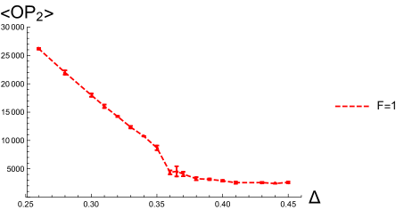
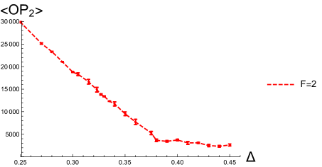
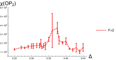
Using the order parameter defined in Eq. (4) we also analyse the impact of the scalar fields on the position of the phase transition line. Once again we fix and vary to find the transition point by looking for peaks in the susceptibility (3). Figure 11 shows the mean values of the order parameter and susceptibility as functions of for CDT including 1, 2 and 3 massless scalar fields. The peak value of indicates that the (pseudo)-critical value of seems to be largely independent of the number of massless scalar fields, remaining within the range - , which is very close to observed for pure gravity simulations with the same lattice volume (). However, the plots of may suggest that the (pseudo)-critical value of slightly increases in response to an increasing number of scalar fields, although this is far from conclusive given the data presented. To summarise, the data presented in Fig. 11 indicates that adding massless scalar fields to CDT does not significantly alter the position of the transition, suggesting that the bifurcation phase is probably not simply an artifact of the naive pure gravity formulation of CDT.

4 Discussion and conclusions
The approach of causal dynamical triangulations (CDT) has produced a number of important results, however some key questions still remain. Principle among these open problems is whether CDT has a continuum limit. An important step towards answering this question will be to determine whether there exists a second order phase transition that is accessible from within the physically interesting phase , at which point the correlation length becomes infinite so that one can keep observable quantities fixed in physical units while the lattice spacing is taken to zero. In this work we have presented strong evidence that the transition between phases and is greater than first order, therefore presenting a strong candidate for the long sought after second order transition.
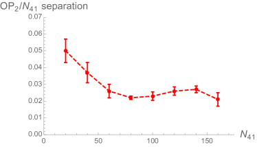
Using an order parameter that exploits the geometric differences in phases and we are able to approximately locate the position of the (pseudo-)critical phase transition for a number of different lattice volumes . By measuring how the position of the phase transition depends on the lattice volume we can extract a value for the critical exponent , which indicates the order of the phase transition. A first order transition is characterised by a critical exponent , whereas for a higher order transition one would expect . Using 8 different lattice volumes we determine the critical exponent of the transition to be . This result marks a significant improvement on the preliminary results found in Ref. [20, 18] and establishes that the transition is greater than first order with a confidence interval. This result strongly supports the conjecture that the phase transition is a higher order transition.
Motivated by Hartle and Hawking’s suggestion that a sufficient number of matter fields may be a necessary condition to produce the correct classical behaviour of the universe [19] we have also investigated the effect of adding massless scalar fields to the bare lattice action of CDT. Specifically, we have studied the impact of scalar fields on average spatial volume profiles and spatial volume fluctuations in the de Sitter phase as well as the bifurcation phase . We observe that the addition of massless scalar fields causes both the volume and fluctuation profiles to narrow in the time direction, with the same qualitative behaviour observed in phases and .
Using the same order parameter studied in the case of pure gravity (zero massless scalar fields) we have also analysed whether the position of the transition line depends on the number of massless scalar fields . We find that the position of the transition appears to be largely independent of the number of massless scalar fields , at least for or . This result may be interpreted as suggesting that the bifurcation phase is probably not simply an artifact of the naive pure gravity formulation of CDT.
Acknowledgements
JGS and JJ wish to acknowledge the support of the grant DEC-2012/06/A/ST2/00389 from the National Science Centre Poland. JA and DNC wish to acknowledge support from the ERC-Advance grant 291092, “Exploring the Quantum Universe” (EQU). AG acknowledges support by the National Science Centre, Poland under grant no. 2015/17/D/ST2/03479.
References
- [1] Marc H. Goroff and Augusto Sagnotti. The Ultraviolet Behavior of Einstein Gravity. Nucl.Phys., B266:709, 1986.
- [2] Gerard ’t Hooft and M.J.G. Veltman. One loop divergencies in the theory of gravitation. Annales Poincare Phys.Theor., A20:69–94, 1974.
- [3] Steven Weinberg. General Relativity, an Einstein Centenary Survey. 1997.
- [4] S. M. Christensen and M. J. Duff. Quantum Gravity in Two + Dimensions. Phys. Lett., B79:213–216, 1978.
- [5] Dario Benedetti, Pedro F. Machado, and Frank Saueressig. Asymptotic safety in higher-derivative gravity. Mod.Phys.Lett., A24:2233–2241, 2009.
- [6] Alessandro Codello, Roberto Percacci, and Christoph Rahmede. Investigating the Ultraviolet Properties of Gravity with a Wilsonian Renormalization Group Equation. Annals Phys., 324:414–469, 2009.
- [7] Daniel F. Litim. Fixed points of quantum gravity. Phys.Rev.Lett., 92:201301, 2004.
- [8] J. Laiho, S. Bassler, D. Coumbe, D. Du, and J. T. Neelakanta. Lattice Quantum Gravity and Asymptotic Safety. arXiv:1604.02745. 2016.
- [9] Jan Ambjorn and R. Loll. Nonperturbative Lorentzian quantum gravity, causality and topology change. Nucl.Phys., B536:407–434, 1998.
- [10] T. Regge. General Relativity Without Coordinates. Nuovo Cim., 19:558–571, 1961.
- [11] J. Ambjørn, J. Gizbert-Studnicki, A. Görlich, J. Jurkiewicz, N. Klitgaard, and R. Loll. Characteristics of the new phase in CDT. Eur. Phys. J., C77(3):152, 2017.
- [12] Jan Ambjorn, Daniel Coumbe, Jakub Gizbert-Studnicki, and Jerzy Jurkiewicz. Recent results in CDT quantum gravity. In 14th Marcel Grossmann Meeting on Recent Developments in Theoretical and Experimental General Relativity, Astrophysics, and Relativistic Field Theories (MG14) Rome, Italy, July 12-18, 2015, 2015.
- [13] J. Ambjorn, A. Gorlich, J. Jurkiewicz, and R. Loll. The Nonperturbative Quantum de Sitter Universe. Phys.Rev., D78:063544, 2008.
- [14] J. Ambjorn, J. Jurkiewicz, and R. Loll. Reconstructing the universe. Phys.Rev., D72:064014, 2005.
- [15] J. Ambjorn, J. Jurkiewicz, and R. Loll. Spectral dimension of the universe. Phys.Rev.Lett., 95:171301, 2005.
- [16] D.N. Coumbe and J. Jurkiewicz. Evidence for Asymptotic Safety from Dimensional Reduction in Causal Dynamical Triangulations. JHEP, 1503:151, 2015.
- [17] Jan Ambjorn, S. Jordan, J. Jurkiewicz, and R. Loll. Second- and First-Order Phase Transitions in CDT. Phys. Rev., D85:124044, 2012.
- [18] D. N. Coumbe, J. Gizbert-Studnicki, and J. Jurkiewicz. Exploring the new phase transition of CDT. JHEP, 02:144, 2016.
- [19] James B. Hartle, S.W. Hawking, and Thomas Hertog. The Classical Universes of the No-Boundary Quantum State. Phys.Rev., D77:123537, 2008.
- [20] Jan Ambjørn, Daniel N. Coumbe, Jakub Gizbert-Studnicki, and Jerzy Jurkiewicz. Signature Change of the Metric in CDT Quantum Gravity? JHEP, 08:033, 2015. [JHEP08,033(2015)].
- [21] J. Ambjorn, A. Goerlich, J. Jurkiewicz, and R. Loll. Nonperturbative Quantum Gravity. Phys.Rept., 519:127–210, 2012.