Impulse-Based Hybrid Motion Control

Abstract

The impulse-based discrete feedback control has been proposed in previous work for the second-order motion systems with damping uncertainties. The sate-dependent discrete impulse action takes place at zero crossing of one of both states, either relative position or velocity. In this paper, the proposed control method is extended to a general hybrid motion control form. We are using the paradigm of hybrid system modeling while explicitly specifying the state trajectories each time the continuous system state hits the guards that triggers impulsive control actions. The conditions for a stable convergence to zero equilibrium are derived in relation to the control parameters, while requiring only the upper bound of damping uncertainties to be known. Numerical examples are shown for an underdamped closed-loop dynamics with oscillating transients, an upper bounded time-varying positive system damping, and system with an additional Coulomb friction damping.

I INTRODUCTION

Hybrid impulsive control [1] combines the piecewise continuous system dynamics with a controlled impulsive behavior, at which a certain jump in the system state occurs at time instants of the discrete impulse action. Both the impulsive control stimulus and, in consequence, resulted state jumps are triggered by the state trajectory hits some prescribed boundary region, therefore fulfilling the so-called guard condition within the state-space. Note that in that case the set of guards constitutes are inherent part of the hybrid control law. Impulsive control obviously belongs to a general framework of the hybrid control systems and, more specifically, provides the system excitation (correspondingly actuation) in form of the infinitely short impulsive stimuli. Despite the methodologies and theoretical examples of the hybrid impulsive and, more generally, switching controls are well-known from the literature e.g. [2, 1, 3] along with fundamentals on the hybrid dynamics and hybrid control systems [4, 5, 6, 7], their applications, in particular in motion control, remain rather modest than one might expect. Not least, a nontrivial analysis and complexity of the associated design methods are responsible for a gap between the theoretical framework of hybrid control systems and their entrance into the engineering practice. In addition, a whole slew of the practical implementation issues, for details we refer to an extensive tutorial [7], make the hybrid control systems to a challenging task for the applications.

Few examples of applying the impulsive control strategies to the motion systems, found in the published works, are mentioned below. An explicit consideration of impulsive control for the motion control systems with uncertain friction has been made in [8]. The authors considered a set-point stabilization for the class of position-, velocity-, and time-dependent friction laws with uncertainty, thus extending an impulsive control strategy originally proposed in [9]. Both approaches [9] and [8] apply the controlled impulsive forces when the system “gets stuck” at non-zero steady-state control error, i.e. when reaching zero velocity in a bounded vicinity to the set-point. Also the use of mechanical stroke impulses for precise alignments of components in the precision engineering and optics has been reported in [10], however without an explicit analysis and design of the control methods. Some neighboring strategies of controllers with a sequence of adapted/modulated pulses, also referred to as dithering, have been former used in the applications, e.g. for positioning tables [11] and pneumatic control valves [12]. Also the experimental evaluation of impulse-based control, similar as addressed in this paper, has been previously shown for the linear guidance drive system in [13].

The aim of this paper is to elaborate the impulsive control method originally proposed in [13] to a general hybrid motion control formulation suitable for the actuated systems with time-varying and uncertain damping characteristics. The outline of the paper is as follows. In Section II, we briefly summarize the impulse-based discrete feedback control, while adapting the control law to be the function of the states rather than time. The hybrid motion control system, in the sense of an autonomous-impulse hybrid system [4], is formulated in Section III while combining the standard proportional-derivative feedback regulator with the proposed impulsive control action aimed for reaching the set-point position despite the damping uncertainties. We provide an explicit analysis of trajectory solutions at zero crossing impulsive control actions and derive the corresponding jump map for the hybrid inclusions. The efficiency of the proposed hybrid motion control is demonstrated in Section IV by three different numerical examples. Finally, some concluding remarks are drawn in Section V.

II IMPULSE-BASED DISCRETE FEEDBACK CONTROL

The impulse-based discrete feedback control has been proposed in [13] for the motion systems with damping uncertainties. The latter assume a relative displacement $x$ with the bounded uncertain damping coefficient $d$ and the known mass $m$. The time-varying damping is driven by some unknown disturbance $\xi(t)$ so that

$$0<\underline{d}\leqslant d(\xi)\leqslant\overline{d}.$$ (1)

The lower and upper bounds of the damping coefficient are indicated by the subscript and superscript correspondingly. Only the upper bound is supposed to be known. The impulse-based discrete feedback control law, similar to the one which is previously used in [13], is given by

$$u=-\alpha\,\mathrm{sign}(\dot{x})\frac{\mathrm{d}}{\mathrm{d}x}\,\mathrm{sign}(x)-\beta\,\mathrm{sign}(x)\frac{\mathrm{d}}{\mathrm{d}\dot{x}}\mathrm{sign}(\dot{x}),$$ (2)

where $\alpha,\,\beta>0$ are the design parameters. Here and further on we will write the dynamic system quantities without explicit time argument, this for the sake of simplicity. Note that unlike in [13], the introduced control law (2) utilizes the sign derivatives with respect to the states and not time argument. This allows a direct relation to the Dirac delta-function used further on in Section III for analysis. Furthermore, we recall that despite the sign operator is not differentiable at zero, in the ordinary sense, its derivative under the generalized notion of differentiation in the distribution theory is twofold of the Dirac $\delta(\cdot)$-function. The later satisfies the identity property of integration over the argument

$$\int\delta(y)dy=1,$$

which we will make use of when analyzing later in Section III the weighted control actions of (2).

The impulsive control action occurs each time the state trajectory crosses one of the state axes so that both summands in (2) are disjunctive. Note that they act simultaneously in zero equilibrium only. Though, when reaching zero equilibrium, the overall control action becomes apparently zero, that follows from the limiting conditions $(x,\dot{x})\rightarrow 0$ substituted into (2) for both possible configurations in the phase-plane, $(x<0,\,\dot{x}>0)$ and $(x>0,\,\dot{x}<0)$. By implication, for any instantaneous point within the state-space except zero equilibrium, both impulsive control summands in (2) can be analyzed independently. In other words, they discrete impulsive execution is joint by the logical operator OR. It is also worth noting that the discrete control system switched at the states zero crossing, also denoted as “twisting algorithm” in [14], has been former proposed in [15] and later analyzed on the finite time convergence and robustness in [16].

III HYBRID MOTION CONTROL SYSTEM

III-A Feedback controlled motion dynamics

Now, consider a hybrid motion control system

$$m\ddot{x}+d(t)\dot{x}=u+v,$$ (3)

with the time-varying damping complying (1), and the control input which combines the impulse-based discrete feedback action (2) and a standard linear feedback regulator $v$. The choice of the latter depends on the eigen-dynamics of system under consideration, i.e. left-hand-side of (3). For instance, without damping uncertainties i.e. $d(t)=\mathrm{const}$ the standard proportional-derivative (PD) control

$$v=K(x_{r}-x)-D\dot{x}$$ (4)

ensures an asymptotic position convergence to the set-point $x_{r}$. Well-known the feedback control gains $K,\,D>0$ allow for arbitrary shaping the second-order closed-loop dynamics. Making the coordinate’s shift to zero set-point, i.e. $x_{r}=0$, the original control problem transforms into that of an unforced motion with non-zero initial condition $x(0)\neq 0$. Substituting (2) and (4) into (3) results in a hybrid motion control system

$$m\ddot{x}+\bigl{(}d(t)+D\bigr{)}\dot{x}+Kx=-\alpha\,\mathrm{sign}(\dot{x})\frac{\mathrm{d}}{\mathrm{d}x}\,\mathrm{sign}(x)-$$

$$-\beta\,\mathrm{sign}(x)\frac{\mathrm{d}}{\mathrm{d}\dot{x}}\mathrm{sign}(\dot{x}).$$ (5)

III-B Autonomous-impulse hybrid system

Generally, an autonomous hybrid (control) system, with a piecewise continuous state dynamics (set-valued flow mapping) $\mathbf{F}:\,\mathcal{C}\rightarrow\mathbb{R}^{n}$ and impulsive behavior (set-valued jump mapping) $\mathbf{J}:\,\mathcal{D}\rightarrow\mathbb{R}^{n}$, can be described by means of the hybrid inclusions [17] as

$$\mathbf{\dot{x}}\in\mathbf{F}(\mathbf{x}) \hbox{ if }\mathbf{x}\in\mathcal{C},$$ (6)

$$\mathbf{x}^{+}\in\mathbf{J}(\mathbf{x}) \hbox{ if }\mathbf{x}\in\mathcal{D}.$$ (7)

Note that the flow set $\mathcal{C}$ and jump set $\mathcal{D}$ should be disjoint in the state-space, i.e. $\mathcal{C}\cap\mathcal{D}=\oslash$. The next state value $\mathbf{x}^{+}$, the so-called “successor”, occurs as a consequence of impulsive control actions which, in conjunction with the system eigen-dynamics, determine the jump mapping $\mathbf{J}$.

Obviously, the hybrid motion control system (5), with the state vector $\mathbf{x}=(x,\dot{x})^{T}$, incorporates only one single-valued flow map so that

$$\mathbf{F}=\{f\}=\left(\begin{array}[]{c}\dot{x}\\[5.69054pt] -\bigl{(}d(t)+D\bigr{)}/m\,\dot{x}-K/m\,x\\ \end{array}\right).$$ (8)

Therefore the flow mapping (6) can be released from the differential inclusion, and the initial hybrid system model can be transformed into

$$\mathbf{\dot{x}}=f(\mathbf{x}) \hbox{ if }\>\mathbf{x}\in\mathcal{C},$$ (9)

$$\mathbf{x}^{+}\in\mathbf{J}(\mathbf{x}) \hbox{ if }\>\mathbf{x}\in\mathcal{D}.$$ (10)

Note that, at the same time, the jump inclusion (10) remains the same as in (7) since the jump mapping incorporates more than one vector-valued function, this according to the right-hand side of (5). Recall that the latter provides an impulsive control stimulus each time the state trajectory hits or crosses one of the state-space axes. This implies

$$\mathcal{D}=X_{0}\cup\dot{X}_{0}\quad\hbox{with}\quad X_{0}:=\{\mathbf{x}\>|\>x=0\},\;\dot{X}_{0}:=\{\mathbf{x}\>|\>\dot{x}=0\},$$

while consequently $\mathcal{C}=\mathbb{R}^{2}\setminus\mathcal{D}$.

In order to derive the jump map of the hybrid motion control system (5), consider the corresponding dynamics for two disjunctive state configurations at zero crossing, i.e. for $J\bigl{(}(0,\dot{x})^{T}\bigr{)}$ and $J\bigl{(}(x,0)^{T}\bigr{)}$. Obviously, for solving the state trajectories and deriving, based thereupon, the jump mapping we can use the linear state-space notation of the system matrix and input coupling vector

$$A=\left(\begin{array}[]{cc}0&1\\[5.69054pt] -\frac{K}{m}&-\frac{d+D}{m}\end{array}\right),\quad B=\left(\begin{array}[]{c}0\\[5.69054pt] \frac{1}{m}\end{array}\right),$$ (11)

given the left-hand-side of (5). The general trajectory solution of (5) can be then written as

$$\mathbf{x}(t)=\exp(At)\,\mathbf{x}_{0}+\int\limits_{t_{0}}^{t}\exp\bigl{(}A(t-\tau)\bigr{)}Bz(\tau)d\tau.$$ (12)

Here the right-hand-side of (5) is summarized by $z(t)$ and an initial state $\mathbf{x}_{0}$ is given for time $t_{0}$. Further one should recall that the matrix exponential function is defined as a power series

$$\exp(At)=\sum\limits_{v=0}^{\infty}\frac{(At)^{v}}{v\,!}.$$

It can be shown that for position zero crossing (further denoted with superscript “$0x$”) the general solution (12) transforms into

$$\mathbf{x}^{0x}(t) = \exp(At)\left(\begin{array}[]{c}0\\ \dot{x}_{0}\\ \end{array}\right)+$$

$$+ \int\limits_{t_{0}}^{t}\exp\bigl{(}A(t-\tau)\bigr{)}B\,\mathrm{sign}\bigl{(}\dot{x}(t)\bigr{)}(-2\alpha)\delta(\tau)d\tau.$$

Note that the inhomogeneous part of solution (III-B), i.e. impulse-excited, is sign-specific depending on the motion direction prior to position zero crossing. Further we note that due to equivalence $\delta(x)|_{x=0}=\delta(t)|_{t=t_{0}}=+\infty$ and $\delta(x)|_{x\neq 0}=\delta(t)|_{t>t_{0}}=0$ for the position zero crossing $x(t_{0})=0$ we use the $\delta$-impulse of time argument $\tau$ instead of that of the state, as otherwise required by (2).

Following the same line of argumentation, it can be shown that for velocity zero crossing (further denoted with superscript “$0\dot{x}$”) the general solution (12) results in

$$\mathbf{x}^{0\dot{x}}(t) = \exp(At)\left(\begin{array}[]{c}x_{0}\\ 0\\ \end{array}\right)+$$

$$+ \int\limits_{t_{0}}^{t}\exp\bigl{(}A(t-\tau)\bigr{)}B\,\mathrm{sign}\bigl{(}x(t)\bigr{)}(-c\beta)\delta(\tau)d\tau.$$

Note that despite the system eigen-dynamics, which is determined by (11), ensures an asymptotic convergence to zero equilibrium, the damping uncertainties can lead to a full motion stop at non-zero position. This is in case of the motion gets sticking or creeping, at which no efficient velocity zero crossing can be detected and, therefore, an undesirable premature motion stop should be taken into account in (III-B). This case, the corresponding derivative of the sign operator yields the single Dirac impulse, instead of the twofold as in case of an effective zero crossing. The introduced weighting variable $c$ captures this distinction by

$$c=\left\{\begin{array}[]{ll}2&\hbox{if }\>\ddot{x}(t_{0})\neq 0,\\[2.84526pt] 1&\hbox{otherwise.}\\ \end{array}\right.$$ (19)

For deriving the jump map of the hybrid motion control system, i.e. determining the system state $\mathbf{x}^{+}=\mathbf{x}(t^{+})$ (the “successor”) after jump, take the limit condition $t\rightarrow t_{0}$ for which (III-B) and (III-B) can be directly evaluated. Assuming the state trajectory hits the jump set $\mathcal{D}$ at time $t_{0}$, for which the instantaneous state $\mathbf{x}_{0}$ is known, results in

$$\mathbf{x}^{+}=\left\{\begin{array}[]{ll}\mathbf{x}^{0x}(t_{0})&\hbox{if }\>\mathbf{x}(t_{0})\in X_{0},\\[2.84526pt] \mathbf{x}^{0\dot{x}}(t_{0})&\hbox{if }\>\mathbf{x}(t_{0})\in\dot{X}_{0}.\end{array}\right.$$ (20)

This yields, after evaluating (III-B) and (III-B), the jump mapping

$$\mathbf{J}(\mathbf{x})=\left\{\begin{array}[]{ll}\mathbf{x}-2B\,\alpha\,\mathrm{sign}(\dot{x})&\hbox{for }\>\mathbf{x}\in X_{0},\\[2.84526pt] \mathbf{x}-cB\,\beta\,\mathrm{sign}(x)&\hbox{for }\>\mathbf{x}\in\dot{X}_{0}.\end{array}\right.$$ (21)

III-C Impulsive control gains

The selection of impulsive control gains, $\alpha$ and $\beta$, follows straight to the jump map since the latter determines the motion system state immediately after an impulsive control execution.

Consider first the discrete control action at the position zero crossing, for which the instantaneous state is $\mathbf{x}(t_{0})=[0,\dot{x}_{0}]$. Obviously, the desired “successor” should lie in the origin, therefore representing attainment of zero equilibrium. Substituting $\textbf{x}^{+}=\mathbf{0}$ into (21), for the first case $\mathbf{x}\in X_{0}$, and solving with respect to the control gain $\alpha$, results in

$$\alpha=0.5m|\dot{x}_{0}|.$$ (22)

Note that the above situation represents an ideal case of instantaneous velocity change, i.e. assuming infinite accelerations of the moving mass. Since a real system acceleration is bounded and with an actuation force dynamics, (22) represents rather the lower gain boundary, below which the state trajectory cannot, even theoretically, reach zero equilibrium after an impulsive control execution. For determining the upper gain boundary one can show that in case of

$$\alpha=m|\dot{x}_{0}|,$$

the jump map yields the state “successor” $\textbf{x}^{+}=-\textbf{x}(t_{0})$, here theoretically as well i.e. without taking into account the real system accelerations. That is the “successor” state will remain in zero position but accept the opposite-sign velocity of the same magnitude as before the last impulsive control action. Consequentially, the resulted (ideal) trajectory will end up in an infinite time switching cycle between $\pm\dot{x}_{0}$ around zero position. The above consideration allows us to formulate the overall gain criterion as

$$0.5m|\dot{x}_{0}|\leq\alpha<m|\dot{x}_{0}|.$$ (23)

Note that the same parameter criterion has been suggested in [13] for the case of the unity mass and without explicit analysis of the hybrid system dynamics and jump mapping.

Now consider the problem of determining $\beta$-gain for an impulsive control action at the velocity zero crossing. Substituting $\textbf{x}^{+}=\mathbf{0}$ into (21), for the second case $\mathbf{x}\in\dot{X}_{0}$, one can see that no direct solution for attaining zero equilibrium exists. This is since the impulsive, equally as any other, control action is unmatched with the position state jump, correspondingly dynamics. Therefore, the single alternative is in providing the jump to a predefined velocity $\dot{x}^{+}$ at $x(t_{0})\neq 0$ which will afterwards allow reaching zero equilibrium for the trajectory to be driven by the eigen-dynamics of (11). For the critically damped eigen-dynamics, i.e. $(d+D)^{2}=4mK$, the homogenous solution is given by

$$x(t)=C_{1}\exp(\lambda t)+C_{2}\exp(\lambda t)t,$$ (24)

where the real double-pole is

$$\lambda=-(d+D)/(2m).$$

Note that here we write some (nominal) constant damping $d$ which complies with (1). Further we explicitly underline that the feedback controlled system should be critically damped by the assigned derivative feedback control gain $D$. In case the controlled motion system becomes underdamped, and that through the time-varying damping behavior $d(t)$, the trajectory will inevitably hits $X_{0}$ and an impulsive action of the position zero crossing employs as described above. On the contrary, if the controlled motion system becomes overdamped, which implies an undesirable premature motion stop, then this case should be captured by the initial requirement on the upper bound of damping coefficient to be known, cf. with Section II. Taking the time derivative of the homogenous solution (24), which is

$$\dot{x}(t)=C_{1}\lambda\exp(\lambda t)+C_{2}\bigl{(}\lambda t\exp(\lambda t)+\exp(\lambda t)\bigr{)},$$ (25)

and solving for the initial values $\mathbf{x}(0)=[x_{0},0]$ one obtains

$$C_{1}=x_{0},\quad C_{2}=-x_{0}\lambda.$$ (26)

It is obvious that the above constants of the homogenous solution (24), (25) reflect both the initial position and system damping and, therefore, bear the signature of the required initial velocity to be excited through an impulsive control action. Moreover it should be underlined that both constants (26) have been determined for the initial values of the nominal system, i.e. with a known and constant damping $d$. Therefore, the nominal system will asymptotically reach zero equilibrium, after velocity zero crossing, even if neither impulsive control action takes place. Consequentially, when substituting the constants (26) into (25), first a zero initial velocity

$$\dot{x}(0)=C_{1}\lambda+C_{2}=x_{0}\lambda-x_{0}\lambda,$$ (27)

is obtained as expected. However, for an uncertain, correspondingly time-varying, system damping the first $\lambda$-term in (27) becomes uncertain, correspondingly time-varying, while the second one remains fixed by the $C_{2}$ initial value. Therefore, the initial velocity required for ensuring the $\lambda$-uncertain solution (24) can reach zero equilibrium is not longer zero. As assumed in Section II, it is sufficient to know the upper bound of the uncertain system damping so that the first $\lambda$-term in (27) can be computed for the maximal damping value $\bar{d}$. After that (27) can be transformed into

$$\dot{x}(0)=-x_{0}\frac{\bar{d}+D}{2m}+x_{0}\frac{d+D}{2m}=-x_{0}\frac{\bar{d}-d}{2m}.$$ (28)

It is evident that the required velocity jump depends on the position at velocity zero crossing, on the one hand, and difference between the upper bound of the damping coefficient and its nominal value $d$, on the other hand. Since the latter is a-priory unknown and, in worst case, can be infinitesimally low at instant of the velocity zero crossing, the suggested velocity jump is

$$\dot{x}^{+}=-x_{0}\frac{\bar{d}}{2m}.$$ (29)

We stress that (29) captures the case of maximal system damping, while for all lower damping values the resulted motion trajectory will be guaranteed hitting $X_{0}$. Now, substituting (29) into (21), for the second case $\mathbf{x}\in\dot{X}_{0}$, and solving with respect to the $\beta$-gain results in

$$\beta=|x_{0}|\frac{\bar{d}}{2c}.$$ (30)

It should be noted that in order to capture the case when the instantaneous acceleration at velocity zero crossing is unavailable, cf. case difference in (19), the weighting factor $c=1$ can be continuously used. Recall that this ensures the $\beta$-gain to be sufficient also in case of the system sticking, i.e. when a relative motion stops outside of zero equilibrium.

IV NUMERICAL EXAMPLES

The proposed hybrid motion control is demonstrated for two numerical examples provided below. The simulation setup is realized using the Simulink^® software from MathWorks Inc, with the set fixed-step (0.0001) $ode3$ solver, while the trapezoidal method for integration calculus is used.

TABLE I: Parameters of numerical simulation setup

Param.	$m$	$K$	$D$	$F_{c}$	$\underline{d}$	$\overline{d}$	$c$	$\alpha/m/|\dot{x}_{0}|$
Value	0.1	10	0.5	1	0.15	1.5	2	0.6

The control parameters are set according to the developments provided in Section III and all the system simulation parameters are listed in Table I. Note that the parameters are assumed as normalized (unitless), so that the computed system states are correspondingly unitless as well.

In order to provide and appropriate sensation of the resulted system dynamics, the hybrid motion control system (5) is first simulated without impulsive control action, i.e. with zero right-hand-side. The non-zero initial position is set to $x(0)=0.5$ so that the PD feedback control loop forces the state trajectory to converge towards zero equilibrium. A comparison is made for two cases – the lower and upper bounds of the system damping $d$. The resulted trajectories are shown in Fig. 1. Obviously, the case of the upper bound of damping coefficient represents a critically damped response, cf. with Section III-C. The case of the lower bound of damping coefficient offers an oscillating trajectory which converges to zero equilibrium after several periods. Note that the assumed lower and upper bounds of the system damping differ by an order of magnitude, see Table I.

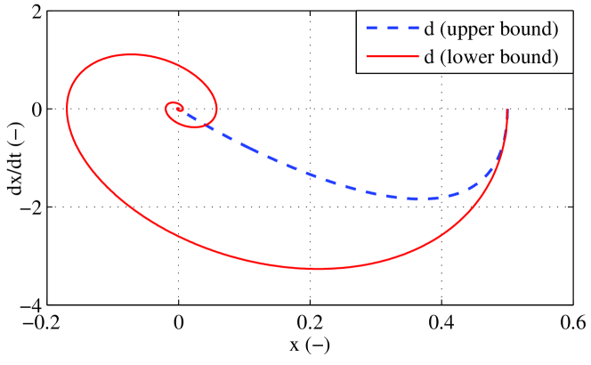
Figure 1: Trajectories of the feedback motion control system (5) without impulsive control part (zero right-hand-side) for initial value $x(0)=0.5$. The system damping at upper $d=\bar{d}=1.5$ and lower $d=\underline{d}=0.15$ bounds.

The above results disclose the reduced performance of the motion control system in case of the underdamped closed-loop dynamics. In the following, we are to evaluate the hybrid motion control system with impulsive control action as in (2).

IV-A Underdamped closed-loop dynamics

When allowing for the impulse-based control law, i.e. employing the right-hand side of (5), the hybrid control performance becomes clearly superior comparing to that demonstrated above for the PD-controlled motion dynamics without impulsive control part.

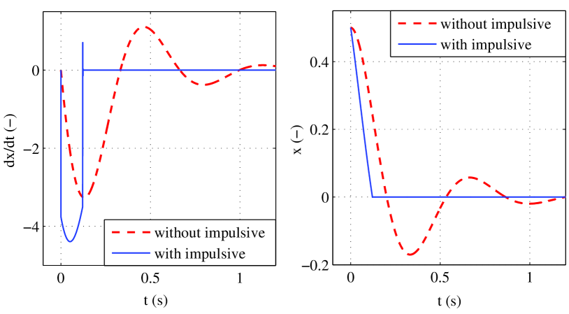
Figure 2: Position and velocity response of the feedback motion control system (5), once with and once without right-hand-side which is impulsive control action. The plant damping of the low bound $d=\underline{d}=0.15$ is assumed.

Here the case of the low bound system damping $d=\underline{d}=0.15$ is assumed, since that one implies several periods of the sate oscillations and, consequently, zero crossing of the state axes at which the impulsive control actions occur. The relative position and velocity response of both motion control systems are shown opposite to each other in Fig. 2. Obviously, the hybrid motion control provides a much faster convergence to zero set-position, even with a nearly linear rate corresponding to the induced velocity. At the same time, the induced peak velocity is not significantly higher comparing to that of the pure PD feedback control. Some minor transient peaks occur in vicinity to zero settling point, but these are fairly negligible comparing to the transient oscillations of the feedback control system without impulsive control part.

IV-B Time-varying damping coefficient

A time-varying system damping $d(t)$ is included into the control system (5) while solely fulfilling the boundary condition (1). The time-varying damping signal is generated by using a low-path filtered white-noise with an additional bias to guarantee that (1) holds. The simulated time-series of the damping coefficient is shown in Fig. 3.

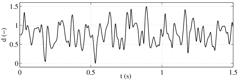
Figure 3: Time-varying damping coefficient used for evaluation.

Note that, generally, a time-varying system damping is usual for e.g. system with mechanical friction, where the weakly-known internal and external factors render the frictional coefficients as time- or state-varying and often without an explicit functional relationship which could assist the control design. For more details on the kinetic friction uncertainties and their impact on the linear feedback control systems we refer to [18] and [19].

The trajectories of the controlled system, once without and once with the impulsive control part, are compared to each other in Fig. 4.

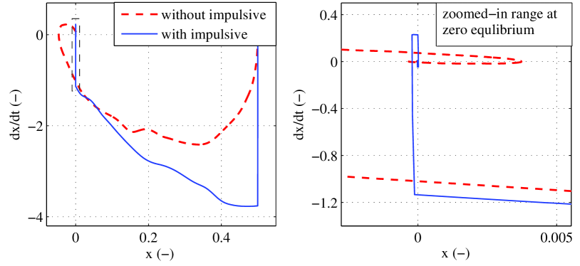
Figure 4: Trajectories of the system (5) with time-varying damping, without and with impulsive control part. The initial value is set to $x(0)=0.5$.

From the zoom-in on the right, it becomes evident that while the first position zero crossing occurs at the comparable velocities, a fast (almost immediate) convergence to zero is only in case of the hybrid impulsive control.

IV-C System with Coulomb friction

The system under control, with the assumed low bound damping $d=\underline{d}=0.15$, is extended by the Coulomb friction so that the left-hand-side of (5) results in $m\ddot{x}+\bigl{(}d(t)+D\bigr{)}\dot{x}+Kx+F_{c}\mathrm{sign}(\dot{x})$. Therefore, the constant friction force of a magnitude equal to the Coulomb friction coefficient $F_{c}>0$ acts at the unidirectional motion, thus providing a rate-independent damping until full motion stop. Well-known, within a certain dead-zone around zero equilibrium, which is $\pm F_{c}/K$ for the PD feedback control (4), the vector field on both sides of the $x$-axis is orthogonal and points towards $\dot{x}=0$. That is once attaining the dead-zone, the trajectory stays for always so that neither continuation of the controlled motion towards zero equilibrium occurs, cf. with [20]. Accordingly, the interval $-F_{c}/K\leq x\leq F_{c}/K$, see grey bar in Fig. 5, constitutes the largest invariant subset of the $x$-axis with an infinite number of stable equilibria. It implies that convergence of the feedback control system to zero equilibrium cannot be guaranteed without impulsive control part, independently of the $K$ and $D$ parameters selection. The corresponding trajectory is shown in Fig. 5 for the initial state $[x(0),\dot{x}(0)]=[0.15,0]$ while the assigned Coulomb friction coefficient results in $F_{c}/K=0.1$.

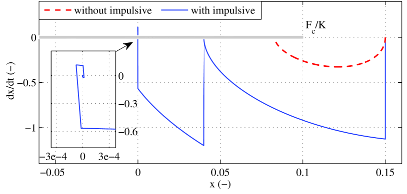
Figure 5: Trajectories of the system (5), extended by Coulomb friction, without and with impulsive control part. The initial position is set to $x(0)=0.15$.

On the contrary, enabling for the impulsive control coaction allows for reaching zero equilibrium, while an asymptotic convergence can be guaranteed. It follows due to zero equilibrium appears as a global attractor as long as $\dot{x},K\neq 0$. Recall that the largest invariant subset lies on the $x$-axis, so that the motion can become ‘stuck’ only at zero velocity. At the same time, an impulsive control action at hitting the $x$-axis ensures the velocity jump so that the system temporary releases from sticking. This is valid even for an infinitesimally short instant as the position approach zero equilibrium, cf. with (26). The trajectory which converges to zero equilibrium when enabling for the impulsive control is equally shown in Fig. 5. One can see that after the first impulse, starting from the same initial position $x(0)=0.15$, the trajectory next reaches the largest invariant subset. Here the system should experience full the motion stop when operating without impulsive control coaction. After hitting the guard, however, the trajectory is repulsed again and runs towards velocity zero crossing. Afterwards the trajectory converges to zero equilibrium while being excited each time when crossing the state axes, see zoom-in in Fig. 5.

V CONCLUSIONS

In this paper we have introduced the generalized formulation of the impulse-based hybrid motion control for the second-order systems with damping uncertainties. Using the unified framework of the hybrid systems and, more specifically, autonomous-impulse hybrid systems, we have analyzed the controlled motion dynamics with the right-hand-side impulsive control actions at both states zero crossing. An appropriate jump inclusion has been derived for the state trajectories hit the guards, which are position and velocity state axes. We have analyzed the “successor” state dynamics, i.e. immediately after execution of impulsive control actions and, based thereupon, provided the appropriate conditions for selection of the control gains. Three numerical examples of the system with (i) significantly underdamped closed-loop dynamics, (ii) time-varying damping, and (iii) additional Coulomb friction damping have been demonstrated to emphasize the performance of the proposed impulse-based hybrid motion control.

References

- [1] B. Miller and E. Rubinovich, Impulsive Control in Continuous and Discrete-Continuous Systems. New-York: Springer US, 2003.
- [2] T. Yang, Impulsive control theory. Berlin: Springer, 2001.
- [3] Z.-H. Guan, D. Hill, and X. Shen, “On hybrid impulsive and switching systems and application to nonlinear control,” IEEE Transactions on Automatic Control, vol. 50, no. 7, pp. 1058–1062, 2005.
- [4] M. Branicky, V. Borkar, and S. Mitter, “A unified framework for hybrid control: model and optimal control theory,” IEEE Transactions on Automatic Control, vol. 43, no. 1, pp. 31–45, 1998.
- [5] R. DeCarlo, M. Branicky, S. Pettersson, and B. Lennartson, “Perspectives and results on the stability and stabilizability of hybrid systems,” Proceedings of the IEEE, vol. 88, no. 7, pp. 1069–1082, 2000.
- [6] W. M. Haddad, V.-S. Chellaboina, and S. G. Nersesov, Impulsive and hybrid dynamical systems. Princeton University Press, 2006.
- [7] R. Goebel, R. Sanfelice, and A. Teel, “Hybrid dynamical systems,” IEEE Control Systems Magazine, vol. 29, no. 2, pp. 28–93, 2009.
- [8] N. Van De Wouw and R. Leine, “Robust impulsive control of motion systems with uncertain friction,” International Journal of Robust and Nonlinear Control, vol. 22, no. 4, pp. 369–397, 2012.
- [9] Y. Orlov, R. Santiesteban, and L. T. Aguilar, “Impulsive control of a mechanical oscillator with friction,” in American Control Conference, 2009, pp. 3494–3499.
- [10] C. Siebenhaar, “Precise adjustment method using stroke impulse and friction,” Precision engineering, vol. 28, no. 2, pp. 194–203, 2004.
- [11] S. Yang and M. Tomizuka, “Adaptive pulse width control for precise positioning under influence of stiction and coulomb friction,” in American Control Conference, 1987, pp. 188–193.
- [12] T. Hägglund, “A friction compensator for pneumatic control valves,” Journal of process control, vol. 12, no. 8, pp. 897–904, 2002.
- [13] M. Ruderman and M. Iwasaki, “Impulse-based discrete feedback control of motion with damping uncertainties,” in IEEE 40th Annual Conference of the Industrial Electronics Society, 2014, pp. 2780–2785.
- [14] L. Fridman, J. A. Moreno, B. Bandyopadhyay, S. Kamal, and A. Chalanga, “Continuous nested algorithms: The fifth generation of sliding mode controllers,” in Recent Advances in Sliding Modes: From Control to Intelligent Mechatronics, 2015, pp. 5–35.
- [15] S. V. Emel’yanov, S. K. Korovin, and L. V. Levantovskii, “Higher-order sliding modes in binary control systems,” Soviet Physics Doklady, vol. 31, no. 7, pp. 291–293, 1986.
- [16] Y. Orlov, “Finite time stability and robust control synthesis of uncertain switched systems,” SIAM Journal on Control and Optimization, vol. 43, no. 4, pp. 1253–1271, 2004.
- [17] J. Lunze and F. Lamnabhi-Lagarrigue, Handbook of hybrid systems control: theory, tools, applications. Cambridge University Press, 2009.
- [18] M. Ruderman and M. Iwasaki, “Observer of nonlinear friction dynamics for motion control,” IEEE Transactions on Industrial Electronics, vol. 62, no. 9, pp. 5941–5949, 2015.
- [19] M. Ruderman, “Integral control action in precise positioning systems with friction,” in IFAC 12th Workshop on Adaptation and Learning in Control and Signal Processing, 2016, pp. 82–86.
- [20] D. Putra, H. Nijmeijer, and N. van de Wouw, “Analysis of undercompensation and overcompensation of friction in 1dof mechanical systems,” Automatica, vol. 43, no. 8, pp. 1387–1394, 2007.