Hidden Broad-line Regions in Seyfert 2 Galaxies: from the spectropolarimetric perspective

Abstract

The hidden broad-line regions (BLRs) in Seyfert 2 galaxies, which display broad emission lines (BELs) in their polarized spectra, are a key piece of evidence in support of the unified model for active galactic nuclei (AGNs). However, the detailed kinematics and geometry of hidden BLRs are still not fully understood. The virial factor obtained from reverberation mapping of type 1 AGNs may be a useful diagnostic of the nature of hidden BLRs in type 2 objects. In order to understand the hidden BLRs, we compile six type 2 objects from the literature with polarized BELs and dynamical measurements of black hole masses. All of them contain pseudobulges. We estimate their virial factors, and find the average value is 0.60 and the standard deviation is 0.69, which agree well with the value of type 1 AGNs with pseudobulges. This study demonstrates that (1) the geometry and kinematics of BLR are similar in type 1 and type 2 AGNs of the same bulge type (pseudobulges), and (2) the small values of virial factors in Seyfert 2 galaxies suggest that, similar to type 1 AGNs, BLRs tend to be very thick disks in type 2 objects.

To appear in The Astrophysical Journal Letters.

1 Introduction

The unified model (Antonucci, 1993), which originates from the detection of broad emission lines (BELs) in the spectropolarimetric data of Seyfert 2 galaxy NGC 1068 (Antonucci & Miller, 1985), proposes that the type 1 (showing both BELs and narrow emission lines) and type 2 (showing only narrow emission lines) active galactic nuclei (AGNs) are the same type of objects viewed from different angles. The hidden broad-line regions (BLRs) are observed in the polarized spectra of many type 2 AGNs (e.g., Antonucci 1984; Tran et al. 1992; Young et al. 1996; Moran et al. 2000; Ramos Almeida et al. 2016), and are thought to have scattering of BELs by the regions above the poles of accretion disks (called “polar scatter regions”) (Antonucci & Miller, 1985; Antonucci, 1993). However, the detailed geometry and kinematics of BLRs hidden in the centers of type 2 AGNs remain elusive and are not yet fully understood.

The virial mass of black holes can be obtained by reverberation mapping (RM, e.g., Blandford & McKee 1982; Peterson et al. 1998; Kaspi et al. 2000; Bentz et al. 2009; Du et al. 2014, 2015, 2016). The RM technique provides a key component, the time lag between continuum and BEL response, that provides a sizescale due to the finite speed of light. There is a dilemma that we are not able to get the black hole mass without specifying the kinematics and structure of the BLR. Fortunately, we can obtain the black hole mass from galactic dynamics in type 2 AGNs, providing the opportunity to define the virial factor

$$f_{\rm vir}=\frac{M_{\bullet}}{M_{\rm vir}}=\frac{GM_{\bullet}}{V^{2}R_{\rm BLR}}$$ (1)

where $M_{\bullet}$ is the BH mass determined by galactic dynamics techniques, $M_{\rm vir}$ is the virial mass, $V$ is the width of BEL, $R_{\rm BLR}$ is the emissivity-weighted radius of BLR, $G$ is the gravitational constant. For type 1 AGNs, $R_{\rm BLR}=c\tau$, where $c$ is the speed of light, $\tau$ is the time delay between the response of broad emission lines (mainly H$\beta$) to the variation of continuum which is normally measured from the peak of cross-correlation functions between the light curves of the continuum and emission lines. The value of virial factor is determined by the geometry and kinematics of BLR, and its evaluation leads to an indirect path to understand the nature of BLRs. Comparing statistically with the BH mass – stellar velocity dispersion ($M_{\bullet}$ – $\sigma_{*}$) relation (e.g., Ferrarese & Merritt 2000; Tremaine et al. 2002), its average value is estimated as the order of unity for type 1 AGNs if the velocity $V$ is measured from the full-width-half-maximum (FWHM) of broad H$\beta$ lines (e.g., Onken et al. 2004; Ho & Kim 2014; Woo et al. 2015). However, a more recent work indicates that the virial factor in individual objects probably varies significantly, as demonstrated by reconstructing the geometry and kinematics of BLRs in a small sample using the Markov Chain Monte Carlo method (MCMC, Pancoast et al. 2014). This result means that the kinematics of BLRs or the viewing angles are diverse in these objects.

The polar scattering regions in type 2 AGNs provides an additional viewing angle, namely from the polar axes, similar to the angle of observation for type 1 AGN. Considering that the virial factor reflects the geometry and kinematics of BLRs, we can diagnose the hidden BLRs in type 2 AGNs by comparing the virial factors, obtained from their polarized spectra, to those of type 1 AGNs. Therefore, we search for type 2 AGNs with hidden BELs in polarized spectra and directly determined dynamical BH mass measurements, and estimate their $f_{\rm vir}$ factors.

2 Virial Factors of Type 2 AGNs

We compile all of the type 2 AGNs which have both polarized BEL detections and direct dynamical BH mass measurements from the published literatures in order to check their virial factors. The objects which are identified definitely as low-ionization nuclear emission-line regions (LINER, e.g., Ho 2008) or those with uncertain BH mass measurements have been eliminated. There are a total of six sources in the final sample. The degree of polarization in type 2 AGNs is generally very low (less than several percent), in most cases, only broad H$\alpha$ lines in the polarized spectra are visible (e.g., Antonucci 1984; Tran et al. 1992; Young et al. 1996; Moran et al. 2000; Ramos Almeida et al. 2016). We assume that broad H$\beta$ and H$\alpha$ lines have the same widths in the polarized spectrum for each individual object, as has been demonstrated in several objects (Ramos Almeida et al., 2016). Because the poor quality of polarized spectra would influence the measurements of the line dispersions (second momentum of the profile, $\sigma$), we only adopt the FWHM of polarized emission lines in the following analysis.

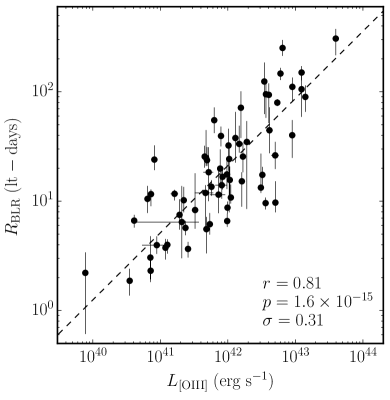
Figure 1: Correlation between the luminosity of [O iii] and $R_{\rm BLR}$. The points with error bars are the RM objects summarized in Du et al. (2015, 2016). The dotted line is the best fit. $r$ is the Pearson’s correlation coefficient, $p$ is null-probability of no correlation and $\sigma$ is the standard deviation of residual after subtracting the best fit in logarithmic space. We adopt $\Lambda$CDM cosmology with $H_{0}=70~{}{\rm km~{}s^{-1}~{}Mpc^{-1}}$, $\Omega_{\Lambda}=0.7$ and $\Omega_{\rm M}=0.3$.

To estimate the radii of BLRs in Equation 1, instead of the RM method as employed for type 1 AGNs, we use of two approaches: (1) the empirical relation between the time delay and the luminosity of [O iii]$\lambda$5007 and (2) the empirical relation with the hard X-ray luminosity in 2-10 keV found in the RM samples. For the first approach, we compile the luminosities of [O iii] and the time delays of H$\beta$ for all of the type 1 AGNs that have RM observations summarized in Du et al. (2015, 2016). It should be noted that the narrow-line regions (NLRs) in type 1 AGNs suffer local extinction of E(B-V) $\sim 0.2-0.3$ (e.g., Netzer et al. 2006; Vaona et al. 2012) in addition to the Galactic extinction (Schlafly & Finkbeiner, 2011). The line extinction should be corrected for the RM objects. Considering that the Balmer decrements of narrow lines for some RM objects are difficult to determine accurately because of their Lorentzian-like H$\alpha$ and H$\beta$ profiles (encompassing both narrow and broad components), we adopt the mean E(B-V) of 0.28, which is obtained from the Data Release 7 quasar sample of Sloan Digital Sky Survey (SDSS, Shen et al. 2011), to correct the intrinsic extinction in those RM objects. Using the FITEXY algorithm (Press et al., 1992) for linear regression, the resulting correlation (shown in Figure 1) is

$$\log R_{\rm BLR}=-(24.475\pm 0.684)+(0.614\pm 0.016)\log L_{\rm[OIII]},$$ (2)

where $L_{\rm[OIII]}$ is the extinction-corrected luminosity of [O iii]. Equation 2 can be used to estimate the BLR radius. In order to avoid the potential contamination of star formation activities in [O iii] fluxes, which would result in uncertainties in $R_{\rm BLR}$ estimates to some extent, we also adopt hard X-ray luminosity in 2-10 keV ($L_{\rm 2-10}$ , the relation of $L_{\rm 2-10}$ versus $R_{\rm BLR}$ in Kaspi et al. 2005) to deduce $R_{\rm BLR}$ as comparison. To calculate the virial factors of the hidden BLRs in type 2 AGN sample, their extinction in narrow emission lines and the absorption in 2-10 keV X-ray luminosities should be also taken into account (see the references in Table 1). The extinction-corrected [O iii] luminosities (corrected individually using the Balmer decrement of NLR for each object found in the literatures) and absorption-corrected hard X-ray luminosities compiled from the literatures, as well as their deduced virial factors (denoted as $f_{\rm[OIII]}$ and $f_{\rm 2-10}$ , respectively), are listed in Table 1.

For the uncertainties of virial factors, the dispersions of the empirical relationships we used are included. For $f_{\rm[OIII]}$ , the primary uncertainties come from the dispersions of Equation 2 (0.31 dex, Figure 1). The uncertainties caused by the [O iii] luminosity measurements are much smaller, and can be ignored. And we use the dispersion (62 percents) of the relation between $L_{\rm 2-10}$ and $R_{\rm BLR}$ (Kaspi et al., 2005) to calculate the error bars of $f_{\rm 2-10}$ . The uncertainties of $L_{\rm 2-10}$ mainly result from their intrinsic variations over time, and have been rolled into the dispersion of the $L_{\rm 2-10}$ – $R_{\rm BLR}$ relationship. Therefore, we do not include them explicitly.

Table 1: Virial factors

Object	FWHM(${\rm H\alpha}$)	Ref.		$M_{\bullet}$	Ref.		$\log L_{\rm[OIII]}^{a}$	Ref.	$f_{\rm[OIII]}$		$\log{L_{\rm 2-10}}$	Ref.	$f_{\rm 2-10}$
	${\rm(km\ s^{-1})}$			$(M_{\odot})$			$(\rm erg\ s^{-1})$				$\rm(erg\ s^{-1})$
Circinus	$2300\pm 500$	1		$1.14^{+0.20}_{-0.20}\times 10^{6}$	2		41.17	3	$0.17^{+0.15}_{-0.15}$		42.62	4	$0.20^{+0.16}_{-0.16}$
IC 2560	$2100\pm 300$	1		$2.51^{+3.80}_{-1.51}\times 10^{6}$	5		40.19	6	$1.83^{+3.11}_{-1.79}$		41.80	7	$1.47^{+2.45}_{-1.34}$
NGC 1068	$4377\pm 300$	8		$8.39^{+0.44}_{-0.44}\times 10^{6}$	9		42.38	4	$0.06^{+0.05}_{-0.05}$		43.02	4	$0.25^{+0.16}_{-0.16}$
NGC 2273	$2399\pm 419$	10b		$8.61^{+0.91}_{-0.46}\times 10^{6}$	11		41.13	4	$1.28^{+1.02}_{-1.02}$		42.73	4	$1.24^{+0.89}_{-0.89}$
NGC 3393	$5000\pm 600$	1		$1.57^{+0.98}_{-0.99}\times 10^{7}$	12		42.04	3	$0.15^{+0.14}_{-0.14}$		41.60	7	$2.08^{+1.90}_{-1.91}$
NGC 4388	$4500\pm 1400$	1		$7.31^{+0.17}_{-0.18}\times 10^{6}$	11		41.85	4	$0.11^{+0.10}_{-0.10}$		42.90	4	$0.24^{+0.21}_{-0.21}$

Note. — References: 1. Ramos Almeida et al. (2016), 2. Greenhill et al. (2003), Kormendy & Ho (2013), 3. Bassani et al. (1999), 4. Marinucci et al. (2012), 5. Läsker et al. (2016), 6. Gu et al. (2006), 7. Tilak et al. (2008), 8. Inglis et al. (1995), 9. Lodato & Bertin (2003), Kormendy & Ho (2013), 10. Moran et al. (2000), 11. Kuo et al. (2011), Kormendy & Ho (2013), 12. Kondratko et al. (2008), Kormendy & Ho (2013). ^aThe Galactic and local extinction has been corrected. ^bWe measure the FWHM from the polarized spectrum in Ref. 10. We do not list the uncertainties of $L_{\rm[OIII]}$ and $L_{\rm 2-10}$ here, because we only use the dispersion of the empirical relationship to deduce the uncertainties of $f_{\rm[OIII]}$ and $f_{\rm 2-10}$ (see Section 2).

The comparison between the virial factors $f_{\rm[OIII]}$ and $f_{\rm 2-10}$  and their distributions are provided in Figure 2. The mean values of $f_{\rm[OIII]}$ and $f_{\rm 2-10}$ are 0.60 and 0.92, and their standard deviations are 0.69 and 0.73, respectively. The Kolmogorov – Smirnof test shows the probability is 8% (It means, if the two distributions were identical, they would appear as discrepant as the observations indicate by chance in 8% of the cases). Considering that the size of the present sample is quite small and the scatter is moderately large, we think the resulting $f_{\rm[OIII]}$ and $f_{\rm 2-10}$ in the present sample are not significantly inconsistent with each other. More observations are needed to clarify this point. The empirical relation between $L_{\rm 2-10}$ and $R_{\rm BLR}$ we used to deduce $f_{\rm 2-10}$ has more uncertainty (Kaspi et al., 2005), we prefer to use $f_{\rm[OIII]}$ in the following discussion.

We individually corrected the extinction of $L_{\rm[OIII]}$ for the six type 2 AGNs (see the references in Table 1), but we adopt a characteristic E(B-V) value to establish the $R_{\rm BLR}$ - $L_{\rm[OIII]}$ relation for the RM AGNs. This characteristic correction method applies to a considerable size sample: (1) Adopting a characteristic value does not influence the slope of the $R_{\rm BLR}$ - $L_{\rm[OIII]}$ relationship, because the Balmer decrement of NLR does not correlate with [O iii] luminosity (Shen et al., 2011). (2) We have checked the effects of different characteristic extinctions, and find if we change it to 0.18 or 0.38, the $f_{\rm[OIII]}$  only becomes 18% smaller or 22% larger, respectively. These uncertainties are much smaller than the error bars. We searched $({\rm H\alpha/H\beta})_{\rm NLR}$ for the RM sample, and found the values for 20 objects which can be measured from their narrow lines reliably (see Table 2). The median $({\rm H\alpha/H\beta})_{\rm NLR}$ for the 20 objects is 4.29, and the corresponding E(B-V) $=$ 0.31 which is similar to the value (0.28) used here. And also, 0.28 is consistent with the mean NLR extinction reported by Heard & Gaskell (2016) (see their Figure 3). Although we cannot find ${\rm(H\alpha/H\beta)_{\rm NLR}}$ reported for the entirety of the RM sample, there is no evidence that the average E(B-V) for the whole RM sample is significantly different from the value we used here. Therefore, the characteristic extinction is reasonable for the present sample.

Table 2: Balmer Decrements

Object	$({\rm H\alpha}/{\rm H\beta})_{\rm NLR}$	Ref.
SDSS J075101.42+291419.1	6.16	1
Mrk 79	2.68	2

Note. — References: 1. Obtained from the spectrum in SDSS, 2. Obtained from the spectrum in NASA/IPAC Extragalactic Database. (This table is available in its entirety in machine-readable form.)

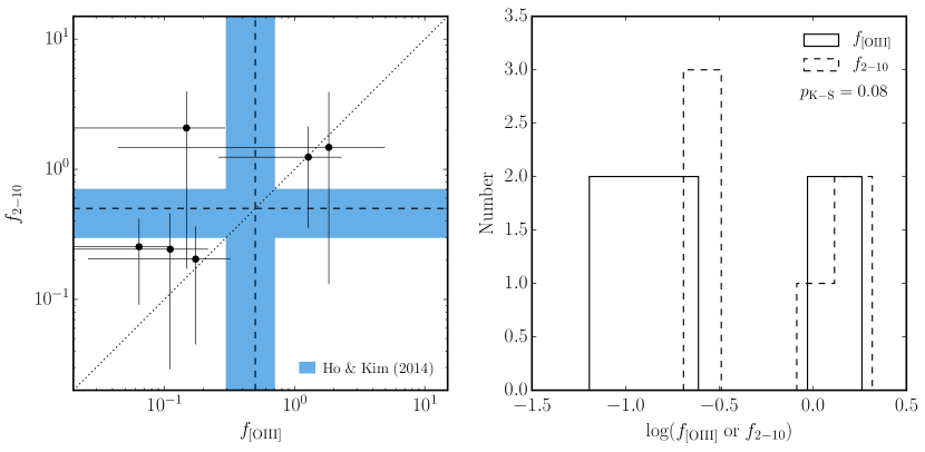
Figure 2: Virial factors. The left panel is the comparison between $f_{\rm[OIII]}$ and $f_{\rm 2-10}$ . The dashed lines and blue regions are the virial factor and its uncertainty for AGNs with pseudobulges in Ho & Kim (2014). The dotted line is the diagonal. The right panel shows the distributions of $f_{\rm[OIII]}$ and $f_{\rm 2-10}$ (solid lines for $f_{\rm[OIII]}$ and dashed lines for $f_{\rm 2-10}$ ). $p_{\rm K-S}$ is the Kolmogorov – Smirnof probability (see Section 2).

3 Comparison with virial factor in type 1 AGNs

In order to compare the obtained virial factors in the type 2 sample with the values in type 1 AGNs, we first provide some necessary background.

Once the time lag between continuum and emission line, as well as the emission line width, have been measured from RM, the mass of BH in an AGN can be determined using Equation 1 if the virial factor $f_{\rm vir}$ is known. Due to the fact that the velocity measurement could be either FWHM or $\sigma$, and the velocity could be measured from mean spectra or rms spectra (Peterson et al., 1998), there are four combinations of $f_{\rm vir}$ estimates ($f_{\rm vir}$ for FWHM in mean or rms spectra, or for $\sigma$ in mean or rms spectra). For simplicity, we designate them as $f_{\rm FWHM}{\rm(mean)}$ , $f_{\rm FWHM}{\rm(rms)}$ , $f_{\rm\sigma}{\rm(mean)}$ and $f_{\rm\sigma}{\rm(rms)}$ .

Assuming the velocity distribution of BLR is isotropic (which is likely not true), the simplest deduction from theory is that the virial factor for FWHM is 0.75 (Netzer, 1990). Observationally, the average virial factor for a sample can be calibrated by comparing the RM objects with measurements of bulge stellar velocity dispersion with the $M_{\bullet}$ – $\sigma_{*}$ relation of inactive galaxies, if we assume that active and inactive galaxies follow the same $M_{\bullet}$ – $\sigma_{*}$ relation. Based on a sample of 14 AGNs with RM observations, Onken et al. (2004) calibrated ${f_{\rm FWHM}{\rm(rms)}}=1.4$ and ${f_{\rm\sigma}{\rm(rms)}}=5.5$ through the comparison with the $M_{\bullet}$ – $\sigma_{*}$relation from Ferrarese & Merritt (2000) and Tremaine et al. (2002). By adding the observations from Lick AGN Monitoring Project (LAMP, e.g., Bentz et al. 2009), Woo et al. (2010) compiled a sample of 24 RM objects with $\sigma_{*}$ measurements and found that $\log{f_{\rm\sigma}{\rm(rms)}}=0.72^{+0.09}_{-0.10}$, if adopting the $M_{\bullet}$ – $\sigma_{*}$relation in Gültekin et al. (2009), which is in good agreement with the value of Onken et al. (2004). Graham et al. (2011) improved the $M_{\bullet}$ – $\sigma_{*}$relation by including more BH mass measurements of barred galaxies, and derived ${f_{\rm\sigma}{\rm(rms)}}=3.8^{+0.7}_{-0.6}$, which is lower than the value in Woo et al. (2010) by a factor of 2, for their sample of 28 AGNs. When dividing the sample into barred and non-barred galaxies, they found $f_{\rm\sigma}{\rm(rms)}$ would be $2.3^{+0.6}_{-0.5}$ and $7.0^{+1.8}_{-1.4}$, respectively. Furthermore, they accounted for the selection bias caused by the non-detection of intermediate-mass BHs, and gave ${f_{\rm\sigma}{\rm(rms)}}=2.8^{+0.7}_{-0.5}$, $2.3^{+0.9}_{-0.6}$ and $5.4^{+1.5}_{-1.2}$ for full, barred and non-barred AGN samples. Park et al. (2012) claimed that the discrepancy of virial factors in those previous works is mainly caused by the sample selection effect, and preferred to use $\log{f_{\rm\sigma}{\rm(rms)}}=0.71\pm 0.11$. Woo et al. (2013) investigated the assumption that active and inactive galaxies follow the same $M_{\bullet}$ – $\sigma_{*}$relation, and demonstrated it is generally reasonable. Grier et al. (2013) updated the RM sample, and added new $\sigma_{*}$ measurements of a few highly-luminous quasars. They obtained ${f_{\rm\sigma}{\rm(rms)}}=4.31\pm 1.05$ which is slightly lower than Park et al.’s value but larger than that in Graham et al. (2011). Motivated by the fact that galaxies with pseudoblges do not obey the $M_{\bullet}$ – $\sigma_{*}$relation of classical bulges and ellipticals, Ho & Kim (2014) separated the calibration by bulge types in galaxies and provided calibrated values of [$f_{\rm FWHM}{\rm(mean)}$ , $f_{\rm\sigma}{\rm(mean)}$ , $f_{\rm FWHM}{\rm(rms)}$ , $f_{\rm\sigma}{\rm(rms)}$ ] = [$1.3\pm 0.4$, $5.6\pm 1.3$, $1.5\pm 0.4$, $6.3\pm 1.5$] for classical bulges and ellipticals, and [$0.5\pm 0.2$, $1.9\pm 0.7$, $0.7\pm 0.2$, $3.2\pm 0.7$] for pseudobulges. More recently, Woo et al. (2015) used the single-epoch spectra and the $R_{\rm BLR}$ – $L_{5100}$ relationship to calibrate narrow-line Seyfert 1 galaxies, and found $\log{f_{\rm FWHM}{\rm(mean)}}=0.05\pm 0.12$ and $\log{f_{\rm\sigma}{\rm(mean)}}=0.65\pm 0.12$.

Based on another technology, Pancoast et al. (2014) carried out MCMC to reconstruct kinematics models of BLRs in five Seyfert 1 galaxies. It does not rely on $M_{\bullet}$ – $\sigma_{*}$ relation, but uses RM data only and can provide $f_{\rm vir}$ estimates for individual objects. Adopting this an independent method, Pancoast et al. (2014) derives the averages $f_{\rm vir}$ for the five objects to be $\approx 0.85$ and $\approx 4.74$ corresponding for FWHM and $\sigma$, respectively. However, the values in individual objects are very different (by an order of magnitude). They also showed that $f_{\rm vir}$ strongly depends on the inclination angle of the BLR and is much larger in more face-on objects (from $\sim 0.2$ for the viewing angle of 50 degrees to $\sim 6$ for 10 degrees).

For the present Seyfert 2 sample, it is difficult to measure the $\sigma$ of emission lines accurately in their polarized spectra given the poor signal-to-noise ratio ($\sigma$ depends on accurate measurement of the wings of emission lines). However, FWHMs are more robustly measured. We only estimate the virial factors based on FWHM. The average value of $f_{\rm vir}$ in those Seyfert 2s is 0.60, and the dispersion is 0.69. Considering that all of the objects in the sample are galaxies with pseudobulges (Kormendy & Ho, 2013), this number is in good agreement with the $f_{\rm FWHM}{\rm(mean)}$ and $f_{\rm FWHM}{\rm(rms)}$ for Seyfert 1 galaxies with pseudobulges in Ho & Kim (2014). Therefore, we can draw a preliminary conclusion, based on the present type 2 sample of limited size, that the virial factors in type 2 AGNs are consistent with the values in type 1 AGNs of the same bulge type (pseudobulge).

Scattering regions in type 2 AGNs are mainly located along the polar axis (e.g., Antonucci 1983; Capetti et al. 1995), and provide a new perspective to BLRs from pole-on direction (small viewing angles). The similar value of virial factors, which are found from the polarized spectra of type 2 AGNs, as in type 1 objects indicate that the geometry and kinematics of BLR are similar in type 1 and type 2 AGNs of the same bulge type (pseudobulge). And the small virial factors (${f_{\rm[OIII]}}=0.60$) found from the polarized spectra demonstrate that the geometry of BLRs in the present sample tend to be very thick disks (thicker than the results in Pancoast et al. 2014 because of our smaller $f_{\rm vir}$) or are perhaps even isotropic to some extent.

It should be noted that thermal motion of the free electrons in scattering regions could provide an additional broadening to the polarized emission lines, and further, influence the estimates of virial factors to some extent. Miller et al. (1991) shows that, consistent with the conclusion of Antonucci & Miller (1985), thermal electrons dominate the scattering process in NGC 1068 and broaden the polarized emission lines. Unfortunately, similar information is unavailable in other AGNs. On the other hand, lower temperature dust grains could also contribute to the scattering, and may dominate at least in some objects. In such case, the additional broadening from the scattering particles is not an issue. The virial factor of NGC 1068 is low compared to the other 5 objects (Table 1). If the width from the dust scattering were used, it would be more similar. The detailed nature of scattering and the corresponding broadening still remain open questions and need to be investigated in the future.

4 Summary

In this work we compile a sample of six Seyfert 2 galaxies with spectropolarimetric observations and dynamical BH mass measurements, and derive their virial factors from the FWHMs of the polarized BELs, in order to investigate the kinematics and geometry of hidden BLRs in type 2 AGNs. Generally, the virial factors estimated in the different ways (from the luminosities of [O iii] and X-ray) are in agreement. The average of the derived virial factors is 0.60 in the present sample, which is similar to the value of type 1 objects with pseudobulges (Ho & Kim, 2014). It implies that (1) the geometry and kinematics of BLR are similar in type 1 and type 2 AGNs of the same bulge type (pseudobulge) and (2) the geometry of BLRs in type 2 AGNs tend to be a very thick disk or isotropic. In the future, more spectropolarimetric observations would make it possible to explore the properties of hidden BLRs in more details, and further, to investigate the dependency of hidden BLR kinematics and geometry on black hole masses or accretion rates of AGNs.

References

- Antonucci (1983) Antonucci, R. R. J. 1983, Nature, 303, 158
- Antonucci (1984) Antonucci, R. R. J. 1984, ApJ, 278, 499
- Antonucci (1993) Antonucci, R. 1993, ARA&A, 31, 473
- Antonucci & Miller (1985) Antonucci, R. R. J., & Miller, J. S. 1985, ApJ, 297, 621
- Bassani et al. (1999) Bassani, L., Dadina, M., Maiolino, R., et al. 1999, ApJS, 121, 473
- Bentz et al. (2009) Bentz, M. C., Walsh, J. L., Barth, A. J., et al. 2009, ApJ, 705, 199
- Blandford & McKee (1982) Blandford, R. D., & McKee, C. F. 1982, ApJ, 255, 419
- Capetti et al. (1995) Capetti, A., Axon, D. J., Macchetto, F., Sparks, W. B., & Boksenberg, A. 1995, ApJ, 446, 155
- Du et al. (2014) Du, P., Hu, C., Lu, K.-X., et al. (SEAMBH Collaboration) 2014, ApJ, 782, 45
- Du et al. (2015) Du, P., Hu, C., Lu, K.-X., et al. (SEAMBH Collaboration) 2015, ApJ, 806, 22
- Du et al. (2016) Du, P., Lu, K.-X., Zhang, Z.-X., et al. (SEAMBH Collaboration) 2016, ApJ, 825, 126
- Fabbiano et al. (2011) Fabbiano, G., Wang, J., Elvis, M., & Risaliti, G. 2011, Nature, 477, 431
- Ferrarese & Merritt (2000) Ferrarese, L., & Merritt, D. 2000, ApJ, 539, L9
- Graham et al. (2011) Graham, A. W., Onken, C. A., Athanassoula, E., & Combes, F. 2011, MNRAS, 412, 2211
- Greenhill et al. (2003) Greenhill, L. J., Booth, R. S., Ellingsen, S. P., et al. 2003, ApJ, 590, 162
- Grier et al. (2013) Grier, C. J., Martini, P., Watson, L. C., et al. 2013, ApJ, 773, 90
- Gu et al. (2006) Gu, Q., Melnick, J., Cid Fernandes, R., et al. 2006, MNRAS, 366, 480
- Gültekin et al. (2009) Gültekin, K., Richstone, D. O., Gebhardt, K., et al. 2009, ApJ, 698, 198
- Heard & Gaskell (2016) Heard, C. Z. P., & Gaskell, C. M. 2016, MNRAS, 461, 4227
- Ho (2008) Ho, L. C. 2008, ARA&A, 46, 475
- Ho & Kim (2014) Ho, L. C., & Kim, M. 2014, ApJ, 789, 17
- Inglis et al. (1995) Inglis, M. D., Young, S., Hough, J. H., et al. 1995, MNRAS, 275, 398
- Kaspi et al. (2005) Kaspi, S., Maoz, D., Netzer, H., et al. 2005, ApJ, 629, 61
- Kaspi et al. (2000) Kaspi, S., Smith, P. S., Netzer, H., et al. 2000, ApJ, 533, 631
- Kormendy & Ho (2013) Kormendy, J., & Ho, L. C. 2013, ARA&A, 51, 511
- Kondratko et al. (2008) Kondratko, P. T., Greenhill, L. J., & Moran, J. M. 2008, ApJ, 678, 87
- Kuo et al. (2011) Kuo, C. Y., Braatz, J. A., Condon, J. J., et al. 2011, ApJ, 727, 20
- Läsker et al. (2016) Läsker, R., Greene, J. E., Seth, A., et al. 2016, ApJ, 825, 3
- Lodato & Bertin (2003) Lodato, G., & Bertin, G. 2003, A&A, 398, 517
- Marinucci et al. (2012) Marinucci, A., Bianchi, S., Nicastro, F., Matt, G., & Goulding, A. D. 2012, ApJ, 748, 130
- Miller et al. (1991) Miller, J. S., Goodrich, R. W., & Mathews, W. G. 1991, ApJ, 378, 47
- Moran et al. (2000) Moran, E. C., Barth, A. J., Kay, L. E., & Filippenko, A. V. 2000, ApJ, 540, L73
- Netzer (1990) Netzer, H. 1990, Active Galactic Nuclei, 57
- Netzer et al. (2006) Netzer, H., Mainieri, V., Rosati, P., & Trakhtenbrot, B. 2006, A&A, 453, 525
- Onken et al. (2004) Onken, C. A., Ferrarese, L., Merritt, D., et al. 2004, ApJ, 615, 645
- Pancoast et al. (2014) Pancoast, A., Brewer, B. J., Treu, T., et al. 2014, MNRAS, 445, 3073
- Park et al. (2012) Park, D., Kelly, B. C., Woo, J.-H., & Treu, T. 2012, ApJS, 203, 6
- Peterson et al. (1998) Peterson, B. M., Wanders, I., Bertram, R., et al. 1998, ApJ, 501, 82
- Press et al. (1992) Press, W. H., Teukolsky, S. A., Vetterling, W. T., & Flannery, B. P. 1992, Cambridge: University Press, —c1992, 2nd ed.,
- Ramos Almeida et al. (2016) Ramos Almeida, C., Martínez González, M. J., Asensio Ramos, A., et al. 2016, MNRAS, 461, 1387
- Schlafly & Finkbeiner (2011) Schlafly, E. F., & Finkbeiner, D. P. 2011, ApJ, 737, 103
- Shen et al. (2011) Shen, Y., Richards, G. T., Strauss, M. A., et al. 2011, ApJS, 194, 45
- Tilak et al. (2008) Tilak, A., Greenhill, L. J., Done, C., & Madejski, G. 2008, ApJ, 678, 701-711
- Tran et al. (1992) Tran, H. D., Miller, J. S., & Kay, L. E. 1992, ApJ, 397, 452
- Tremaine et al. (2002) Tremaine, S., Gebhardt, K., Bender, R., et al. 2002, ApJ, 574, 740
- Vaona et al. (2012) Vaona, L., Ciroi, S., Di Mille, F., et al. 2012, MNRAS, 427, 1266
- Woo et al. (2013) Woo, J.-H., Schulze, A., Park, D., et al. 2013, ApJ, 772, 49
- Woo et al. (2010) Woo, J.-H., Treu, T., Barth, A. J., et al. 2010, ApJ, 716, 269
- Woo et al. (2015) Woo, J.-H., Yoon, Y., Park, S., Park, D., & Kim, S. C. 2015, ApJ, 801, 38
- Young et al. (1996) Young, S., Hough, J. H., Efstathiou, A., et al. 1996, MNRAS, 281, 1206