Structure-preserving model reduction for
marginally stable LTI systems

Abstract

This work proposes a structure-preserving model reduction method for marginally stable linear time-invariant (LTI) systems. In contrast to Lyapunov-stability-based approaches—which ensure the poles of the reduced system remain in the open left-half plane—the proposed method preserves marginal stability by reducing the subsystem with poles on the imaginary axis in a manner that ensures those poles remain purely imaginary. In particular, the proposed method decomposes a marginally stable LTI system into (1) an asymptotically stable subsystem with eigenvalues in the open left-half plane and (2) a pure marginally stable subsystem with a purely imaginary spectrum. We propose a method based on inner-product projection and the Lyapunov inequality to reduce the first subsystem while preserving asymptotic stability. In addition, we demonstrate that the pure marginally stable subsystem is a generalized Hamiltonian system; we then propose a method based on symplectic projection to reduce this subsystem while preserving pure marginal stability. In addition, we propose both inner-product and symplectic balancing methods that balance the operators associated with two quadratic energy functionals while preserving asymptotic and pure marginal stability, respectively. We formulate a geometric perspective that enables a unified comparison of the proposed inner-product and symplectic projection methods. Numerical examples illustrate the ability of the method to reduce the dimensionality of marginally stable LTI systems while retaining accuracy and preserving marginal stability; further, the resulting reduced-order model yields a finite infinite-time energy, which arises from the pure marginally stable subsystem.

1 Introduction

Reduced-order models (ROMs) are essential for enabling high-fidelity computational models to be used in many-query and real-time applications such as control, optimization, and uncertainty quantification. Marginally stable linear time-invariant dynamical (LTI) systems often arise in such applications; examples include inviscid fluid flow, quantum mechanics, and undamped structural dynamics. An ideal model-reduction approach for such systems would produce a dynamical-system model that is lower dimensional, is accurate with respect to the original model, and remains marginally stable, which is an intrinsic property of the dynamical system (it ensures, e.g., a finite system response at infinite time). Unfortunately, most classical model-reduction methodologies, such as balanced truncation [34], Hankel norm approximation [19], optimal $\mathcal{H}_{2}$ approximation [20, 48, 32], and Galerkin projection exploiting inner-product structure [43], were originally developed for asymptotically stable LTI systems, i.e., systems with all poles in the open left half-plane.

Although developed for asymptotically stable systems, balanced truncation and optimal $\mathcal{H}_{2}$ approximation can be extended to unstable stable systems without poles on the imaginary axis. In particular, a reduced-order model can be obtained by balancing and truncating frequency-domain controllability and observability Gramians [41, 51]. By extending the $\mathcal{H}_{2}$ norm to the $\mathcal{L}_{2}$-induced Hilbert-Schmidt norm, an iteratively corrected rational Krylov algorithm was proposed for optimal $\mathcal{L}_{2}$ model reduction [31]. However, the methods in Refs. [41, 51, 31] cannot be applied to marginally stable systems, as the frequency-domain controllability and observability Gramians as well as the $\mathcal{L}_{2}$-induced Hilbert-Schmidt norm are not well defined when there are poles on the imaginary axis.

Although many well-known model reduction methods can be directly applied to systems with purely imaginary poles, they do not guarantee stability. These methods include proper orthogonal decomposition (POD)–Galerkin [24], balanced POD [42], pseudo balanced POD [30, 36], and moment matching [5, 18]. The shift-reduce-shift-back approach (SRSB) [50, 8, 44, 52, 49] reduces a $\mu$-shifted system $(A-\mu I,B,C)$ by balanced truncation. However, this approach fails to ensure stability when the balanced reduced system is shifted back by $\mu$.

In general, stability-preserving ROMs fall into roughly two categories. The first category of methods derives a priori a stability-preserving model reduction framework, often specific to a particular equation set; the present work falls within this category. Refs. [43, 9, 25] construct ROMs in an energy-based inner product. Ref. [45] extends Ref. [9, 25] by applying the stabilizing projection to a skew-symmetric system constructed by augmenting a given linear system with its dual system. Refs. [28, 12, 13, 46, 22, 40, 21, 38, 37, 1] construct reduced-order models to preserve the Lagrangian and (port-)Hamiltonian structures of the original systems. However, these methods cannot be applied to general marginally stable LTI systems.

The second category of methods stabilizes an unstable ROM through a posteriori stabilization step. In particular, Ref. [26] stabilizes reduced-order models via optimization-based eigenvalue reassignment. Refs. [11, 2, 6] construct reduced basis via minimal subspace rotation on the Stiefel manifold while preserving certain properties of the original system matrix. Other methods includes to introduce viscosity [4, 39, 16] or penalty term [14], to enrich basis functions representing the small and energy dissipation scale [7, 35, 10], and to calibrate POD coefficients [15, 27]. In many cases, the stabilization alters the original unstable ROM and a sacrifice of accuracy is inevitable.

In this work, we propose a structure-preserving model-reduction method for marginally stable systems. The method guarantees marginal-stability preservation by executing two steps. First, the approach decomposes the original marginally stable linear system into two subsystems: one with eigenvalues in the left-half plane and one with nonzero eigenvalues on the imaginary axis. This is similar to the approach taken in Ref. [33, 51] for performing model reduction of unstable systems without poles on the imaginary axis. Specifically, given a marginally stable (autonomous) LTI system $\dot{x}=Ax$, where $A$ is invertible and all eigenvalues have a non-positive real part, we apply a similarity transformation, which yields $A=T\mathop{\operator@font diag}\nolimits(A_{s},A_{m})T^{-1}$. Here, $A_{s}$ has eigenvalues in the left-half plane (i.e., is Hurwitz) and $A_{m}$ has purely imaginary eigenvalues. In this case, the subsystem $\dot{x}_{s}=A_{s}x_{s}$ is asymptotically stable, while we show that the subsystem $\dot{x}_{m}=A_{m}x_{m}$ is a generalized Hamiltonian system. Second, the method performs structure-preserving model reduction on the subsystems separately; namely, inner-product projection based on the Lyapunov inequality is employed to reduce the asymptotically stable subsystem, while symplectic projection is applied to the pure marginally stable subsystem characterized by purely imaginary eigenvalues.

Specific contributions of this work include:

1. A novel structure-preserving model reduction method for marginally stable LTI systems that preserves the asymptotic stability of the asymptotically stable subsystem via inner-product projection and the pure marginal stability of pure marginally stable subsystem via symplectic projection (Algorithm 1).

2. A general inner-product projection framework (Section 3), which we demonstrate ensures asymptotic-stability preservation if the matrix used to define the inner product satisfies the Lyapunov inequality (Lemma 11).

3. An inner-product balancing approach that enables the operators associated with any primal or dual quadratic energy functional to be balanced (Section 3.4). If either of these satisfies a Lyapunov inequality, then asymptotic stability is additionally preserved (Corollary 15). We show that many existing model-reduction techniques (e.g., POD–Galerkin, balanced truncation, balanced POD, and SRSB) can be expressed as an inner-product projection and in fact are special cases of inner-product balancing (Table 3).

4. A stabilization approach that produces an asymptotically stable reduced-order model starting with a subset of the ingredients required for a stability-preserving inner-product projection, e.g., starting with an arbitrary trial basis matrix and a symmetric-positive-definite matrix that satisfies the Lyapunov inequality (Section 3.5).

5. Analysis that demonstrates that any pure marginally stable system is equivalent to a generalized Hamiltonian system with marginal stability (Theorem 27).

6. A novel symplectic-projection framework (Section 4) that ensures preservation of pure marginal stability (Theorem 34).

7. A symplectic balancing approach that enables the operators associated with any primal or negative dual quadratic energy functional to be balanced (Section 4.4) and preserve pure marginal stability (Corollary 38). In particular, we show that the generalized Hamiltonians associated with the primal and negative dual systems can be balanced with this approach.

8. A stabilization approach that produces a pure marginally stable reduced-order model starting with a subset of the ingredients required for a symplectic projection (Section 4.5).

9. A geometric framework that enables a unified analysis and comparison of inner-product and symplectic projection (Tables 1 and 2).

10. Experiments on two model problems that demonstrate that the proposed method has a small relative error in both the state and total energy (Section 5). Because symplectic model reduction is energy-conserving, the proposed method ensures that the infinite-time system energy is equal to the initial energy of the marginally stable subsystem. In contrast, the infinite-time energy of other reduced models is zero or infinity.

The remainder of the paper is organized as follows. Section 2 provides an overall view of the proposed method. Sections 3 and 4 present the methodologies to reduce the asymptotically stable subsystem and marginally stable subsystem, respectively. Section 5 illustrates the stability, accuracy, and efficiency of the proposed method through two numerical examples. Finally, Section 6 provides conclusions.

We make extensive use of the following sets in the remainder of the paper:

• $\mathrm{SPD}(n)$: the set of all $n\times n$ symmetric-positive-definite (SPD) matrices.

• $\mathrm{SPSD}(n)$: the set of all $n\times n$ symmetric-positive-semidefinite (SPSD) matrices.

• $\mathrm{SS}(n)$: the set of $n\times n$ nonsingular, skew-symmetric matrices.

• $\mathrm{H}(n)$: the set of real-valued $n\times n$ matrices whose eigenvalues have strictly negative real parts (i.e., the set of Hurwitz matrices).

• $\mathrm{GH}(n)$: the set of real-valued $n\times n$ diagonalizable matrices with nonzero purely imaginary eigenvalues.

• $\mathbb{R}_{*}^{n\times k}$: the set of full-column-rank $n\times k$ matrices with $k\leq n$ (i.e., the non-compact Stiefel manifold).

• $O(M,N)$: the set of full-column-rank $n\times k$ matrices $V$ with $k\leq n$ such that $V^{\tau}MV=N$ with $M\in\mathrm{SPD}(n)$ and $N\in\mathrm{SPD}(k)$. Note that $O(I_{n},I_{k})$ represents the Stiefel manifold.

• $\mathrm{Sp}(J_{\Omega},J_{\Pi})$: the set of full-column-rank $2n\times 2k$ matrices $V$ with $k\leq n$ such that $V^{\tau}J_{\Omega}V=J_{\Pi}$ with $J_{\Omega}\in\mathrm{SS}(2n)$ and $J_{\Pi}\in\mathrm{SS}(2k)$. Note that $\mathrm{Sp}(J_{2n},J_{2k})$ represents the symplectic Stiefel manifold.

2 Marginally stable LTI systems

We begin by formulating the full-order model, which is a marginally stable LTI system (Section 2.1), and subsequently present the formulation for a general projection-based reduced-order model (Section 2.2). Then, we present the proposed framework based on system decomposition (Section 2.3).

2.1 Full-order model

This work considers continuous-time LTI systems of the form

(1) $$\dot{x} =Ax+Bu$$

$$y =Cx$$

with $A\in\mathbb{R}^{n\times n}$, $B\in\mathbb{R}^{n\times p}$, and $C\in\mathbb{R}^{q\times n}$, $x\in\mathbb{R}^{n}$, $u\in\mathbb{R}^{p}$, and $y\in\mathbb{R}^{q}$. We denote this system by $(A,B,C)$ and focus on the particular case where the linear system is marginally stable. Because stability concerns the spectrum of the operator $A$, we focus primarily on the corresponding autonomous system

(2) $$\dot{x}=Ax.$$

We now define marginal stability.

Definition 1 (Marginal stability).

Linear system (1) is marginally stable, or Lyapunov stable, if for every initial condition $x(0)=x_{0}\in\mathbb{R}^{n}$, the state response $x(t)$ of the associated autonomous system (2) is uniformly bounded.

The following standard lemmas (e.g., Ref. [23, pp. 66–70]) provide conditions for marginal stability.

Lemma 2.

The following conditions are equivalent:

1. The system (1) is marginally stable.

2. All eigenvalues of $A$ have non-positive real parts and all Jordan blocks corresponding to eigenvalues with zero real parts are $1\times 1$.

Lemma 3.

The system (1) is marginally stable if one of the following conditions holds:

1. There exists $\Theta\in\mathrm{SPD}(n)$ that satisfies the Lyapunov inequality

   (3) $$A^{\tau}\Theta+\Theta A\preceq 0.$$

2. For every $Q\in\mathrm{SPSD}(n)$, there exists a unique solution $\Theta\in\mathrm{SPD}(n)$ to the Lyapunov equation

   (4) $$A^{\tau}\Theta+\Theta A=-Q.$$

3. There exists $\Theta\in\mathrm{SPD}(n)$ such that the energy $\frac{1}{2}x^{\tau}\Theta x$ of the corresponding autonomous system is nonincreasing in time, i.e.,

   (5) $$\frac{d}{dt}\left(\frac{1}{2}x^{\tau}\Theta x\right)\leq 0,$$

   for $x\in\mathbb{R}^{n}$ satisfying (2).

We note that because $\frac{d}{dt}(\frac{1}{2}x^{\tau}\Theta x)=\frac{1}{2}x^{\tau}(A^{\tau}\Theta+\Theta A)x$, (a) and (c) are equivalent. Lemma 3 provides sufficient conditions for marginal stability; not all marginally stable systems have a Lyapunov matrix $\Theta$ that satisfies (3)–(5).

2.2 Reduced-order model

Let $\Psi,\Phi\in\mathbb{R}_{*}^{n\times k}$ denote test and trial basis matrices that are biorthogonal (i.e., $\Psi^{\tau}\Phi=I_{k}$) and whose columns span $k$-dimensional test and trial subspaces of $\mathbb{R}^{n}$, respectively. If the reduced-order model is constructed via Petrov–Galerkin projection performed on the full-order model, then (1) reduces to

(6) $$\dot{z} =\tilde{A}z+\tilde{B}u$$

$$y =\tilde{C}z,$$

where $\tilde{A}{:=}\Psi^{\tau}A\Phi\in\mathbb{R}^{k\times k}$, $\tilde{B}{:=}\Psi^{\tau}B\in\mathbb{R}^{k\times p}$, $\tilde{C}{:=}C\Phi\in\mathbb{R}^{q\times k}$, and the state is approximated as $x\approx\Phi z$. We denote this system by $(\tilde{A},\tilde{B},\tilde{C})$. The corresponding autonomous system is

(7) $$\dot{z}=\tilde{A}z$$

with initial condition $z(0)=\Psi^{\tau}x_{0}\in\mathbb{R}^{k}$.

2.3 System decomposition

If the full-order-model system (1) is marginally stable and the matrix $A$ has a full rank, then there exists $T\in\mathbb{R}_{*}^{n\times n}$ such that the similarity transformation satisfies

(8) $$A=T\begin{bmatrix}A_{s}&0\\ 0&A_{m}\end{bmatrix}T^{-1},$$

where $A_{s}\in\mathrm{H}(n_{s})$, $A_{m}\in\mathrm{GH}(n_{m})$, and $n_{s}+n_{m}=n$. Let $T=\begin{bmatrix}T_{s}&T_{m}\end{bmatrix}$ with $T_{s}\in\mathbb{R}_{*}^{n\times n_{s}}$ and $T_{m}\in\mathbb{R}_{*}^{n\times n_{m}}$. Then, $AT_{i}=T_{i}A_{i}$ (for $i\in\{s,m\}$), which implies that the columns of $T_{i}$ span an invariant subspace of $A$. Let $x_{s}\in\mathbb{R}^{n_{s}}$ and $x_{m}\in\mathbb{R}^{n_{m}}$. Substituting $x=T\begin{bmatrix}x_{s}^{\tau}&x_{m}^{\tau}\end{bmatrix}^{\tau}$ into (1) and premultiplying the first set of equations by $T^{-1}$ yields a decoupled LTI system

(9) $$\begin{split}\frac{d}{dt}\begin{bmatrix}x_{s}\\ x_{m}\end{bmatrix}&=\begin{bmatrix}A_{s}&0\\ 0&A_{m}\end{bmatrix}\begin{bmatrix}x_{s}\\ x_{m}\end{bmatrix}+\begin{bmatrix}B_{s}\\ B_{m}\end{bmatrix}u\\ y&=\begin{bmatrix}C_{s}&C_{m}\end{bmatrix}\begin{bmatrix}x_{s}\\ x_{m}\end{bmatrix},\end{split}$$

where $T^{-1}B=\begin{bmatrix}B_{s}^{\tau}&B_{m}^{\tau}\end{bmatrix}^{\tau}$ and $CT=\begin{bmatrix}C_{s}&C_{m}\end{bmatrix}$. Here, the subsystem associated with $x_{s}$ is asymptotically stable, while the subsystem associated with $x_{m}$ is marginally stable.

This decomposition enables each subsystem to be reduced in a manner that preserves its particular notion of stability. In the present context, we can accomplish this by defining biorthogonal test and trial basis matrices for each subsystem $\Psi_{i}\in\mathbb{R}_{*}^{n_{i}\times k_{i}}$, $\Phi_{i}\in\mathbb{R}_{*}^{n_{i}\times k_{i}}$, $i\in\{s,m\}$. Applying Petrov–Galerkin projection to (9) with test basis matrix $\mathop{\operator@font diag}\nolimits(\Psi_{s},\Psi_{m})$ and trial basis matrix $\mathop{\operator@font diag}\nolimits(\Phi_{s},\Phi_{m})$ yields a decoupled reduced LTI system

(10) $$\begin{split}\frac{d}{dt}\begin{bmatrix}z_{s}\\ z_{m}\end{bmatrix}&=\begin{bmatrix}\tilde{A}_{s}&0\\ 0&\tilde{A}_{m}\\ \end{bmatrix}\begin{bmatrix}z_{s}\\ z_{m}\end{bmatrix}+\begin{bmatrix}\tilde{B}_{s}\\ \tilde{B}_{m}\end{bmatrix}u\\ y&=\begin{bmatrix}\tilde{C}_{s}&\tilde{C}_{m}\end{bmatrix}\begin{bmatrix}z_{s}\\ z_{m}\end{bmatrix},\end{split}$$

where the full state is approximated as

$$x(t)\approx T\begin{bmatrix}\Phi_{s}z_{s}(t)\\ \Phi_{m}z_{m}(t)\end{bmatrix}.$$

Within this decomposition-based approach, basis matrices $\Psi_{s}$ and $\Phi_{s}$ can be computed to preserve asymptotic stability in the associated reduced subsystem (e.g., via balanced truncation or other Lyapunov methods). For the marginally stable subsystem, we will show that the symplectic model reduction method can be applied to obtain a low-order marginally stable system wherein all eigenvalues of $\tilde{A}_{m}$ are nonzero and purely imaginary.

Algorithm 1 summarizes the proposed procedure for computing reduced-order-model operators $(\tilde{A}_{s},\tilde{B}_{s},\tilde{C}_{s})$ and $(\tilde{A}_{m},\tilde{B}_{m},\tilde{C}_{m})$. Here, we have defined Table 1 lists the methods and key properties of each subsystem. The next two sections explain Algorithm 1 and Table 1 in detail.

Algorithm 1 Structure-preserving model reduction for marginally stable LTI systems.

0:  A marginally stable LTI system $(A,B,C)$.

0:  Reduced-order-model operators $(\tilde{A}_{s},\tilde{B}_{s},\tilde{C}_{s})$ and $(\tilde{A}_{m},\tilde{B}_{m},\tilde{C}_{m})$.

1:  Compute a matrix $T$ such that $A$ is transformed into block-diagonal form (8).

2:  Select $M\in\mathrm{SPD}(n_{s})$ such that the Lyapunov inequality $A_{s}^{\tau}M+MA_{s}\prec 0$ is satisfied.

3:  Construct trial basis matrix $\Phi_{s}\in O(M,N)$ for some $N\in\mathrm{SPD}(k_{s})$, $k_{s}<n_{s}$.

4:  Construct test basis matrix $\Psi_{s}=M\Phi_{s}N^{-1}$.

5:  Construct the reduced system $\tilde{A}_{s}=\Psi_{s}^{\tau}A_{s}\Phi_{s}$, $\tilde{B}_{s}=\Psi_{s}^{\tau}B_{s}$, $\tilde{C}_{s}=C_{s}\Phi_{s}$.

6:  Select $J_{\Omega}\in\mathrm{SS}(n_{m})$ such that $A_{m}=-J_{\Omega}^{-1}L$ with $L\in\mathrm{SPD}(n_{m})$.

7:  Construct trial basis matrix $\Phi_{m}\in\mathrm{Sp}(J_{\Omega},J_{\Pi})$ for some $J_{\Pi}\in\mathrm{SS}(k_{m})$, $k_{m}<n_{m}$.

8:  Construct test basis matrix $\Psi_{m}=J_{\Omega}\Phi_{m}J_{\Pi}^{-1}$.

9:  Construct the reduced system $\tilde{A}_{m}=\Psi_{m}^{\tau}A_{m}\Phi_{m}$, $\tilde{B}_{m}=\Psi_{m}^{\tau}B_{m}$, $\tilde{C}_{m}=C_{m}\Phi_{m}$.

Appendix A describes how this decomposition approach can be extended to general unstable LTI systems with $A$ possibly singular.

Table 1: Inner-product model reduction v. symplectic model reduction.

	Asymptotically stable subsystem	Marginally stable subsystem
Original space	Inner-product space: $(\mathbb{R}^{n_{s}},M)$ with $M\in\mathrm{SPD}(n_{s})$	Symplectic space: $(\mathbb{R}^{n_{m}},J_{\Omega})$ with $J_{\Omega}\in\mathrm{SS}(n_{m})$
System matrix	$A_{s}\in\mathrm{H}(n_{s})$	$A_{m}\in\mathrm{GH}(n_{m})$
Autonomous system	$\dot{x}_{s}=A_{s}x_{s}$ with $x_{s}\in\mathbb{R}^{n_{s}}$	$\dot{x}_{m}=A_{m}x_{m}$ with $x_{m}\in\mathbb{R}^{n_{m}}$
Key property of full system	Lyapunov inequality: $A_{s}^{\tau}M+MA_{s}\prec 0$	Generalized Hamiltonian property: $A_{m}^{\tau}J_{\Omega}+J_{\Omega}A_{m}=0$
Energy property of full system	$\frac{d}{dt}\left(\frac{1}{2}x_{s}^{\tau}Mx_{s}\right)<0$	$\frac{d}{dt}\left(\frac{1}{2}x_{s}^{\tau}Lx_{s}\right)=0$ with $A_{m}=-J_{\Omega}^{-1}L$
Canonical form	$M=I_{n}$ $A_{s}^{\tau}+A_{s}\prec 0$	$J_{\Omega}=J_{2n}$ $A_{m}^{\tau}J_{2n}+J_{2n}A_{m}=0$
Reduced space	Inner-product space: $(\mathbb{R}^{k_{s}},N)$ with $N\in\mathrm{SPD}(k_{s})$	Symplectic space: $(\mathbb{R}^{k_{m}},J_{\Pi})$ with $J_{\Pi}\in\mathrm{SS}(k_{m})$
Projection	Inner-product projection	Symplectic projection
Trial basis matrix	$\Phi_{s}\in O(M,N)$	$\Phi_{m}\in\mathrm{Sp}(J_{\Omega},J_{\Pi})$
Test basis matrix	$\Psi_{s}=M\Phi_{s}N^{-1}\in\mathbb{R}_{*}^{n_{s}\times k_{s}}$	$\Psi_{m}=J_{\Omega}\Phi_{m}J_{\Pi}^{-1}\in\mathbb{R}_{*}^{n_{m}\times k_{m}}$
Reduced-system matrix	$\tilde{A}_{s}=\Psi_{s}^{\tau}A_{s}\Phi_{s}\in\mathrm{H}(k_{s})$	$\tilde{A}_{m}=\Psi_{m}^{\tau}A_{m}\Phi_{m}\in\mathrm{GH}(k_{m})$
Reduced autonomous system	$\dot{z}_{s}=\tilde{A}_{s}z_{s}$	$\dot{z}_{m}=\tilde{A}_{m}z_{m}$
Key property of reduced system	Lyapunov inequality: $\tilde{A}_{s}^{\tau}N+N\tilde{A}_{s}\prec 0$	Generalized Hamiltonian property: $\tilde{A}_{m}^{\tau}J_{\Pi}+J_{\Pi}\tilde{A}_{m}=0$
Energy property of reduced system	$\frac{d}{dt}\left(\frac{1}{2}z_{s}^{\tau}Nz_{s}\right)<0$	$\frac{d}{dt}\left(\frac{1}{2}z_{s}^{\tau}\tilde{L}z_{s}\right)=0$ with $\tilde{A}_{m}=-J_{\Pi}^{-1}\tilde{L}$
Approximate solution	$x_{s}(t)\approx\Phi_{s}z_{s}(t)$	$x_{m}(t)\approx\Phi_{m}z_{m}(t)$

3 Reduction of asymptotically stable subsystems

This section focuses on reducing the asymptotically stable subsystem $\dot{x}_{s}=A_{s}x_{x}$. Section 3.2 introduces inner-projection projection, Section 3.3 demonstrates that a model-reduction method based on inner-projection projection preserves asymptotic stability, Section 3.4 presents the inner-product-balancing framework, and Section 3.5 describes methods for constructing the basis matrices that lead to a inner-product projection given a subset of the required ingredients. For notational simplicity, we omit the subscript $s$ throughout this section.

3.1 Asymptotically stable systems

We begin by defining asymptotic stability.

Definition 4 (Asymptotic stability).

Linear system (1) is asymptotically stable if, in addition to being marginally stable, $x(t)\to 0$ as $t\to\infty$ for every initial condition $x(0)=x_{0}\in\mathbb{R}^{n}$.

In analogue to Lemmas 2–3, we now provide conditions for asymptotic stability.

Lemma 5.

The following conditions are equivalent:

1. The system (1) is asymptotically stable.

2. $A\in\mathrm{H}(n)$.

3. There exists $\Theta\in\mathrm{SPD}(n)$ that satisfies the Lyapunov inequality

   (11) $$A^{\tau}\Theta+\Theta A\prec 0.$$

4. For every $Q\in\mathrm{SPD}(n)$, there exists a unique Lyapunov matrix $\Theta\in\mathrm{SPD}(n)$ that satisfies (4).

5. There exists $\Theta\in\mathrm{SPD}(n)$ such that the energy $\frac{1}{2}x^{\tau}\Theta x$ of the corresponding autonomous system is strictly decreasing in time, i.e.,

   (12) $$\frac{d}{dt}\left(\frac{1}{2}x^{\tau}\Theta x\right)<0,$$

   for any $x\neq 0\in\mathbb{R}^{n}$ satisfying (2).

We note that $A\in\mathrm{H}(n)$ does not necessarily imply that the symmetric part of $A$ is negative definite. However, $A\in\mathrm{H}(n)$ if and only if it can be transformed into a matrix with negative symmetric part by similarity transformation with a real matrix; see Lemma 41 in Appendix B for details.

We now connect asymptotic stability of the primal system to that of its dual.

Lemma 6 (Dual version of Lemma 5).

If any condition of Lemma 5 holds, then the following conditions hold:

1. The dual system $(A^{\tau},C^{\tau},B^{\tau})$ is asymptotically stable.

2. $A^{\tau}\in\mathrm{H}(n)$.

3. There exists $\Theta^{\prime}\in\mathrm{SPD}(n)$ that satisfies the dual Lyapunov inequality

   (13) $$A\Theta^{\prime}+\Theta^{\prime}A^{\tau}\prec 0.$$

4. For every $Q^{\prime}\in\mathrm{SPD}(n)$, there exists a unique Lyapunov matrix $\Theta^{\prime}\in\mathrm{SPD}(n)$ that satisfies

   (14) $$A\Theta^{\prime}+\Theta^{\prime}A^{\tau}=-Q^{\prime}.$$

5. There exists $\Theta^{\prime}\in\mathrm{SPD}(n)$ such that the energy $\frac{1}{2}x^{\tau}\Theta^{\prime}x$ of the corresponding autonomous dual system is strictly decreasing in time, i.e.,

   (15) $$\frac{d}{dt}\left(\frac{1}{2}x^{\tau}\Theta^{\prime}x\right)<0,$$

   for any $x\neq 0\in\mathbb{R}^{n}$ satisfying $\dot{x}=A^{\tau}x$.

Proof.

Because the eigenvalues of $A$ are identical to the eigenvalues of $A^{\tau}$, $A\in\mathrm{H}(n)$ if and only if $A^{\tau}\in\mathrm{H}(n)$. Thus the LTI system associated with $A^{\tau}$ is asymptotically stable and satisfies the corresponding conditions of Lemma 5. ∎

Remark 7 (Relationship with negative dual system: asymptotic stability).

Thus, any method proposed in this work for ensuring asymptotic stability of a given (sub)system also ensures asymptotic stability of the associated dual (sub)system. However, because the trial basis $\Phi$ associated with $(\tilde{A},\tilde{B},\tilde{C})$ corresponds to the test basis of $(\tilde{A}^{\tau},\tilde{C}^{\tau},\tilde{B}^{\tau})$ (i.e., $\tilde{A}^{\tau}=\Phi^{\tau}A^{\tau}\Psi$), the proposed methods for constructing a trial basis matrix $\Phi$ should be applied to the dual system as a test basis matrix. Similarly, the proposed methods for constructing a test basis matrix $\Psi$ should be applied to the dual system as a trial basis matrix.

3.2 Inner-product projection of spaces

Let $\mathbb{V}\cong\mathbb{R}^{n}$ and $\mathbb{W}\cong\mathbb{R}^{k}$ with $k\leq n$ denote vector spaces equipped with inner products $\left\langle\cdot,\cdot\right\rangle_{\mathbb{V}}:\mathbb{V}\times\mathbb{V}\to\mathbb{R}$ and $\left\langle\cdot,\cdot\right\rangle_{\mathbb{W}}:\mathbb{W}\times\mathbb{W}\to\mathbb{R}$ respectively. These inner products can be represented by matrices $M\in\mathrm{SPD}(n)$ and $N\in\mathrm{SPD}(k)$, respectively, i.e.,

$$\left\langle\hat{x}_{1},\hat{x}_{2}\right\rangle_{\mathbb{V}} \equiv x_{1}^{\tau}Mx_{2},\quad\forall x_{1},x_{2}\in\mathbb{R}^{n}$$

$$\left\langle\hat{z}_{1},\hat{z}_{2}\right\rangle_{\mathbb{W}} \equiv z_{1}^{\tau}Nz_{2},\quad\forall z_{1},z_{2}\in\mathbb{R}^{k},$$

where the operator $\hat{\cdot}$ provides the representation of an element of a vector space from its coordinates, i.e., $\hat{x}\in\mathbb{V}$, $\forall x\in\mathbb{R}^{n}$ and $\hat{z}\in\mathbb{W}$, $\forall z\in\mathbb{R}^{k}$. We represent these inner-product spaces $\mathbb{V}$ and $\mathbb{W}$ by $(\mathbb{R}^{n},M)$ and $(\mathbb{R}^{k},N)$ respectively.

Definition 8 (Inner-product lift).

An inner-product lift is a linear mapping $\phi:\mathbb{W}\to\mathbb{V}$ that preserves inner-product structure:

(16) $$\left\langle\hat{z}_{1},\hat{z}_{2}\right\rangle_{\mathbb{W}}=\left\langle\phi(\hat{z}_{1}),\phi(\hat{z}_{2})\right\rangle_{\mathbb{V}},\quad\forall\hat{z}_{1},\hat{z}_{2}\in\mathbb{W}.$$

Definition 9 (Inner-product projection).

Let $\phi:\mathbb{W}\to\mathbb{V}$ be an inner-product lift. The adjoint of $\phi$ is the linear mapping $\psi:\mathbb{V}\to\mathbb{W}$ satisfying

(17) $$\left\langle\psi(\hat{x}),\hat{z}\right\rangle_{\mathbb{W}}=\left\langle\hat{x},\phi(\hat{z})\right\rangle_{\mathbb{V}},\quad\forall\hat{z}\in\mathbb{W},\ \hat{x}\in\mathbb{V}.$$

We say $\psi$ is the inner-product projection induced by $\phi$.

In coordinate space, this inner-product lift and projection can be expressed equivalently as

$$\phi(\hat{z}) \equiv\Phi z,\quad\forall z\in\mathbb{R}^{k}$$

$$\psi(\hat{x}) \equiv\Psi^{\tau}x,\quad\forall x\in\mathbb{R}^{n},$$

respectively, where (16)–(17) imply that $\Phi\in\mathbb{R}_{*}^{n\times k}$ and $\Psi\in\mathbb{R}_{*}^{n\times k}$ satisfy

(18) $$\Phi^{\tau}M\Phi =N$$

(19) $$\Psi N =M\Phi,$$

from which it follows that

(20) $$\Psi=M\Phi N^{-1}.$$

For convenience, we write $\Phi\in O(M,N)$. Although $\Psi^{\tau}$ is not in general equal to the Moore–Penrose pseudoinverse $(\Phi^{\tau}\Phi)^{-1}\Phi^{\tau}$, it can be verified that it is indeed a left inverse of $\Phi$, which implies that $\psi\circ\phi$ is the identity map on $\mathbb{W}$.

3.3 Inner-product projection of dynamics

This section describes the connection between inner-product projection and asymptotic-stability preservation in model reduction. Namely, we show that if inner-product projection is employed to construct the reduced-order model with $M$ corresponding to a Lyapunov matrix of the original system, then the reduced-order model inherits asymptotic stability.

Definition 10 (Model reduction via inner-product projection).

A reduced-order model $(\tilde{A},\tilde{B},\tilde{C})$ with $\tilde{A}=\Psi^{\tau}A\Phi$, $\tilde{B}=\Psi^{\tau}B$, and $\tilde{C}=C\Phi$ is constructed by an inner-product projection if $\Phi\in O(M,N)$, $\Psi=M\Phi N^{-1}$, where $M\in\mathrm{SPD}(n)$ and $N\in\mathrm{SPD}(k)$.

Lemma 11 (Inner-product projection preserves asymptotic stability).

If the original LTI system $(A,B,C)$ has a Lyapunov matrix $\Theta$ satisfying (11) and the reduced-order model is constructed by inner-product projection with $M=\Theta$, then the reduced-order model $(\tilde{A},\tilde{B},\tilde{C})$ is asymptotically stable with Lyapunov matrix $N$.

Proof.

Left- and right-multiplying inequality (11) (with $\Theta=M$) by $\Phi^{\tau}$ and $\Phi$, respectively, yields

(21) $$\Phi^{\tau}A^{\tau}M\Phi+\Phi^{\tau}MA\Phi\prec 0.$$

Substituting (19) and $\tilde{A}=\Psi^{\tau}A\Phi$ in (21) yields

(22) $$\tilde{A}^{\tau}N+N\tilde{A}\prec 0,$$

which implies that the reduced system is asymptotically stable by Lemma 5. ∎

We note that Lemma 11 is a generalization of the stability-preservation property in Ref. [43], which required the reduced space to be Euclidean (i.e., $N=I_{k}$ in the present notation). Lemma 11 considers a more general form where the reduced space can be any inner-product space, i.e., $N\in\mathrm{SPD}(k)$ but otherwise arbitrary.

3.4 Inner-product balancing

We now describe an inner-product-balancing approach that leverages inner-product structure. Table 2 compares this approach with a novel symplectic-balancing approach, which will be described in Section 4.4.

Table 2: Inner-product balancing v. symplectic balancing. Both methods require inputs $\Xi,\Xi^{\prime}\in\mathrm{SPD}(n)$ and employ decompositions $\Xi=RR^{\tau}$, $\Xi^{\prime}=SS^{\tau}$, and $R^{\tau}S=U\Sigma V^{\tau}$ and $\bar{\Phi}=SV_{1}\Sigma_{1}^{-1/2}$, $\bar{\Psi}=RU_{1}\Sigma_{1}^{-1/2}$.

	Inner-product balancing	Symplectic balancing
Primal energy $\frac{1}{2}x^{\tau}Mx$	$M=\Xi$	$M=G^{-\tau}\mathop{\operator@font diag}\nolimits(\Xi,\Xi^{\prime})G^{-1}$
Dual energy $\frac{1}{2}(x^{\prime})^{\tau}M^{\prime}x^{\prime}$	$M^{\prime}=\Xi^{\prime}$	$M^{\prime}=G\mathop{\operator@font diag}\nolimits(\Xi^{\prime},\Xi)G^{\tau}$
Autonomous dual system	$\dot{x}^{\prime}=A^{\tau}x^{\prime}$	$\dot{x}^{\prime}=-A^{\tau}x^{\prime}$
Trial basis $\Phi$	$\Phi=\bar{\Phi}$	$\Phi=G\mathop{\operator@font diag}\nolimits(\bar{\Phi},\bar{\Psi})$
Test basis $\Psi$	$\Psi=\bar{\Psi}$	$\Psi=G^{-\tau}\mathop{\operator@font diag}\nolimits(\bar{\Psi},\bar{\Phi})$
Structure	Inner-product projection with $M=\Xi$, $M^{\prime}=\Xi^{\prime}$, $N=N^{\prime}=\Sigma_{1}$	Symplectic projection with $J_{\Omega}=-J_{\Omega^{\prime}}^{-1}=G^{-\tau}J_{2n}G^{-1}$, $J_{\Pi}=J_{\Pi^{\prime}}=J_{2k}$
Balancing property	$\Phi\in O(M,\Sigma_{1})$ $\Psi\in O(M^{\prime},\Sigma_{1})$	$\Phi\in O(M,\mathop{\operator@font diag}\nolimits(\Sigma_{1},\Sigma_{1}))$ $\Psi\in O(M^{\prime},\mathop{\operator@font diag}\nolimits(\Sigma_{1},\Sigma_{1}))$
Canonical choice for energies $\Xi$ and $\Xi^{\prime}$	$\Xi=W_{o}$, $\Xi^{\prime}=W_{c}$	$\Xi=\Xi^{\prime}=\beta$
Stability preserved	Asymptotic stability if $A^{\tau}\Xi+\Xi A\prec 0$ or $A\Xi^{\prime}+\Xi^{\prime}A^{\tau}\prec 0$	Pure marginal stability if $A=JL$ with $J=-J_{\Omega}^{-1}$ and $L\in\mathrm{SPD}(2n)$

Definition 12 (Inner-product balancing).

Given any $\Xi\in\mathrm{SPD}(n)$ and $\Xi^{\prime}\in\mathrm{SPD}(n)$, the trial and test basis matrices characterizing an inner-product balancing correspond to

(23) $$\Phi=SV_{1}\Sigma_{1}^{-1/2}\quad\text{and}\quad\Psi=RU_{1}\Sigma_{1}^{-1/2},$$

respectively, where $\Xi=RR^{\tau}$, $\Xi^{\prime}=SS^{\tau}$, and $R^{\tau}S=U\Sigma V^{\tau}$ is the singular value decomposition. Here, we have defined $U=[U_{1}\ U_{2}]$, $\Sigma=\mathop{\operator@font diag}\nolimits(\Sigma_{1},\Sigma_{2})$, and $V=[V_{1}\ V_{2}]$, where $U_{1},V_{1}\in O(I_{n},I_{k})$ and $\Sigma_{1}=\mathop{\operator@font diag}\nolimits(\sigma_{1},\ldots,\sigma_{k})$ contains the $k$ largest singular values of $R^{\tau}S$.

We now show that inner-product balancing leads to an inner-product projection.

Lemma 13.

An inner-product balancing characterized by the test and trial basis matrices $(\Psi,\Phi)$ with $\Xi,\Xi^{\prime}\in\mathrm{SPD}(n)$ has the following properties:

1. The basis matrices $(\Psi,\Phi)$ correspond to an inner-product projection performed on an LTI system $(A,B,C)$ with $M=\Xi$ and $N=\Sigma_{1}$.

2. The basis matrices $(\Phi,\Psi)$ correspond to an inner-product projection performed on the dual system $(A^{\tau},C^{\tau},B^{\tau})$ with $M^{\prime}=\Xi^{\prime}$ and $N^{\prime}=\Sigma_{1}$.

3. The basis matrices $(\Psi,\Phi)$ balance $\Xi$ and $\Xi^{\prime}$, i.e., $\Phi\in O(\Xi,\Sigma_{1})$ and $\Psi\in O(\Xi^{\prime},\Sigma_{1})$.

Proof.

To prove (a), we verify that $\Phi\in O(\Xi,\Sigma_{1})$ and $\Psi=\Xi\Phi\Sigma_{1}^{-1}$, as

$$\Phi^{\tau}\Xi\Phi=\left(SV_{1}\Sigma_{1}^{-1/2}\right)^{\tau}\left(RR^{\tau}\right)\left(SV_{1}\Sigma_{1}^{-1/2}\right)=\left(\left(R^{\tau}S\right)V_{1}\Sigma_{1}^{-1/2}\right)^{\tau}\left(\left(R^{\tau}S\right)V_{1}\Sigma_{1}^{-1/2}\right)=\Sigma_{1},$$

$$\Xi\Phi\Sigma_{1}^{-1}=\left(RR^{\tau}\right)\left(SV_{1}\Sigma_{1}^{-1/2}\right)\Sigma_{1}^{-1}=RU_{1}\Sigma_{1}^{-1/2}=\Psi.$$

Thus, the conditions for an inner-product projection are satisfied; note that $\Psi^{\tau}\Phi=I_{k}$. To prove (b), recall from Remark 7 that the test basis of the dual system corresponds to $\Phi$, while the trial basis corresponds to $\Psi$. Thus, we aim to verify that $\Psi\in O(\Xi^{\prime},\Sigma_{1})$ and $\Phi=\Xi^{\prime}\Psi\Sigma_{1}^{-1}$, which can be done similarly to the steps above. Finally, (c) holds because $\Phi\in O(\Xi,\Sigma_{1})$ and $\Psi\in O(\Xi^{\prime},\Sigma_{1})$. ∎

We now show that any inner-product projection corresponds to a particular balancing.

Lemma 14.

If test and trial basis matrices $(\Psi,\Phi)$ characterize an inner-product projection with $M\in\mathrm{SPD}(n)$ and $N\in\mathrm{SPD}(n)$, then there exists $M^{\prime}\in\mathrm{SPD}(n)$ such that $\Phi\in O(M,N)$ and $\Psi\in O(M^{\prime},N)$. Further, there exists a realization of that reduced-order model that corresponds to an inner-product balancing with $\Xi=M$, $\Xi^{\prime}=\hat{M}^{\prime}$, and $\Sigma_{1}=\mathop{\operator@font diag}\nolimits(\lambda_{1},\ldots,\lambda_{k})$ characterized by basis matrices $(\hat{\Psi},\hat{\Phi})$ that satisfy $\hat{\Phi}\in O(M,\Lambda)$, $\text{Ran}(\Phi)=\text{Ran}(\hat{\Phi})$, $\hat{\Psi}\in O(\hat{M}^{\prime},\Lambda)$, $\text{Ran}(\Psi)=\text{Ran}(\hat{\Psi})$, and $\Psi^{\tau}\Phi=\hat{\Psi}^{\tau}\hat{\Phi}=I_{k}$.

Proof.

From the definition of an inner-product projection, we have $\Phi\in O(M,N)$ and $\Psi=M\Phi N^{-1}$. Using $M^{\prime}=\Psi_{\mathrm{ext}}^{-\tau}N_{\mathrm{ext}}\Psi_{\mathrm{ext}}^{-1}$, we have $[\Psi\ \bar{\Psi}]^{\tau}M^{\prime}[\Psi\ \bar{\Psi}]=\mathop{\operator@font diag}\nolimits(N,\bar{N})$, whose (1,1) block gives $\Psi\in O(M^{\prime},N)$. Similarly, $\Phi^{\tau}M\Phi=N$ implies $U^{\tau}\Phi^{\tau}M\Phi U=\Lambda$, thus $\Phi\in O(M,N)$ implies $\hat{\Phi}\in O(M,\Lambda)$ with $\hat{\Phi}=\Phi U$. Using $\hat{M}^{\prime}=\hat{\Psi}_{\mathrm{ext}}^{-\tau}\hat{N}_{\mathrm{ext}}\hat{\Psi}_{\mathrm{ext}}^{-1}$, we have $[\hat{\Psi}\ \bar{\Psi}]^{\tau}\hat{M}^{\prime}[\hat{\Psi}\ \bar{\Psi}]=\mathop{\operator@font diag}\nolimits(\Lambda,\bar{N})$, whose (1,1) block gives $\hat{\Psi}\in O(M^{\prime},\Lambda)$. Now, to ensure $(\hat{\Psi},\hat{\Phi})$ corresponds to an inner-product projection with $M$ and $\Lambda$, we set $\hat{\Psi}=M\hat{\Phi}\Lambda^{-1}=M\Phi U\Lambda^{-1}=M\Phi N^{-1}NU\Lambda^{-1}=\Psi NU\Lambda^{-1}$. Noting that $\text{Ran}(\Phi)=\text{Ran}(\hat{\Phi})$ and $\text{Ran}(\Psi)=\text{Ran}(\hat{\Psi})$ as well as $\Psi^{\tau}\Phi=\hat{\Psi}^{\tau}\hat{\Phi}=I_{k}$, we conclude that basis matrices $(\Psi,\Phi)$ and $(\hat{\Psi},\hat{\Phi})$ yield different realizations of the same reduced-order model. ∎

Corollary 15.

A inner-product-balancing reduced-order model preserves asymptotic stability if $\Theta=\Xi$ satisfies the Lyapunov inequality (11), or if $\Theta^{\prime}=\Xi^{\prime}$ satisfies the dual Lyapunov inequality (13).

Proof.

The result follows directly from Lemmas 13 (a) and 11, as Lemma 13 (b) and 11 for the dual system. ∎

We note that many existing model-reduction methods correspond to an inner-product balancing; these methods are reported in Table 3. Appendix E discusses these model-reduction methods in more detail.

Table 3: Comparison of different model-reduction methods with inner-product-balancing structure defined by $\Xi$ and $\Xi^{\prime}$. In all cases, $N=\Sigma_{1}$ is defined by the inner-product balancing. The remaining quantities are defined in Appendix E.

	POD–Galerkin	Balanced truncation	Balanced POD	SRSB	Proposed inner-product projection
$M=\Xi$	$XX^{\tau}$	$W_{o}$	$\hat{W}_{o}$	$W_{o}^{\mu}$	$\Theta$ satisfying (11)
$M^{\prime}=\Xi^{\prime}$	$XX^{\tau}$	$W_{c}$	$\hat{W}_{c}$	$W_{c}^{\mu}$	$\Theta^{\prime}$ satisfying (13)
Stability preservation?	No	Yes	No	No	Yes

3.5 Construction of basis matrices given subset of ingredients

Lemma 11 demonstrated that a ROM will preserve asymptotic stability if it is constructed via inner-product projection with $M=\Theta$ a Lyapunov matrix satisfying (11). Unfortunately, as reported in Table 3, while many typical model-reduction techniques associate with an inner-product projection (and an inner-product balancing), the associated operator $M$ does not often satisfy the Lyapunov inequality, which precludes assurances of stability preservation (e.g., POD–Galerkin, Balanced POD, and SRSB).

We propose three methods (including inner-product balancing) for constructing a stability-preserving inner-product projection satisfying the conditions of Lemma 11. Table 4 summarizes these methods; this corresponds to Steps 6–8 in Algorithm 1. Methods 2 and 3 assume that we are given a subset of the required ingredients, which can be computed by any technique. For example, the trial basis can be computed by POD, balanced POD, or rational approximation; the metric $\Theta$ can be obtained by solving Lyapunov equation (4) with $Q\in\mathrm{SPD}(n)$ but otherwise arbitrary. Thus, these methods can be viewed as stabilization techniques applied to the provided inputs.

Table 4: Algorithms for constructing an inner-product projection that ensure the conditions of Definition 10.

	Method 1 (inner-product balancing)	Method 2	Method 3
Input	$\Xi,\Xi^{\prime}\in\mathrm{SPD}(n)$ with $\Xi=\Theta$ satisfying (11) or $\Xi^{\prime}=\Theta^{\prime}$ satisfying (13)	$\Phi\in\mathbb{R}_{*}^{n\times k}$, $\Theta$ satisfying (11)	$\Phi_{0}\in O(M_{0},N_{0})$, $N_{0},N\in\mathrm{SPD}(k)$, $M_{0}\in\mathrm{SPD}(n)$, $\Theta$ satisfying (11)
Output	$M\in\mathrm{SPD}(n)$, $N\in\mathrm{SPD}(k)$, $\Phi\in O(M,N)$, $\Psi\in O(M^{\prime},N)$	$M\in\mathrm{SPD}(n)$, $N\in\mathrm{SPD}(k)$, $\Psi\in\mathbb{R}_{*}^{n\times k}$	$M\in\mathrm{SPD}(n)$, $\Phi\in O(M,N)$, $\Psi\in\mathbb{R}_{*}^{n\times k}$
Algorithm	1. Compute symmetric factorization     $\Xi=RR^{\tau}$, $\Xi^{\prime}=SS^{\tau}$ 2. Compute SVD $R^{\tau}S=U\Sigma V^{\tau}$ 3. $\bar{\Phi}=SV_{1}\Sigma_{1}^{-1/2}$ 4. $\bar{\Psi}=RU_{1}\Sigma_{1}^{-1/2}$ 5. $M=\Xi$, $M^{\prime}=\Xi^{\prime}$, $N=\Sigma_{1}$	1. $M=\Theta$ 2. $N=\Phi^{\tau}M\Phi$ 3. $\Psi=M\Phi N^{-1}$	1. Set $M=\Theta$ 2. Construct $G\in O(M,M_{0})$ 3. Construct $\tilde{G}\in O(N,N_{0})$ 4. $\Phi=G\Phi_{0}\tilde{G}^{-1}$ 5. $\Psi=M\Phi N^{-1}$

Method 2 constructs a stability-preserving inner-product projection starting with any arbitrarily chosen trial basis matrix $\Phi\in\mathbb{R}_{*}^{n\times k}$ and a Lyapunov matrix $\Theta$ satisfying (11). Method 3 constructs a stability-preserving inner-product projection starting with a basis $\Phi_{0}\in O(M_{0},N_{0})$, where $M_{0}$ might not satisfy Lyapunov inequality (11), and a Lyapunov matrix $\Theta$ satisfying (11). For simplicity, we can choose $G=M^{-1/2}M_{0}^{1/2}$ and $\tilde{G}=N^{-1/2}N_{0}^{1/2}$. Lemma 16 demonstrates that we can compute the trial basis matrix in this context as $\Phi=G\Phi_{0}^{\tau}\tilde{G}^{-1}\in O(M,N)$, which constitutes step 4 of the algorithm.

Lemma 16.

Let $\phi:(\mathbb{R}^{k},N)\to(\mathbb{R}^{n},M),x\mapsto\Phi x$ denote an inner-product lift with $\Phi\in O(M,N)$. Let $g:(\mathbb{R}^{n},M_{0})\to(\mathbb{R}^{n},M),x\mapsto Gx$ and $\tilde{g}:(\mathbb{R}^{k},N_{0})\to(\mathbb{R}^{k},N),x\mapsto\tilde{G}x$ represent (invertible) inner-product transformations, i.e., $G\in O(M,M_{0})\subseteq\mathbb{R}_{*}^{n\times n}$ and $\tilde{G}\in O(N,N_{0})\subseteq\mathbb{R}_{*}^{k\times k}$, respectively. Then, there exists a unique inner-product lift $\phi_{0}:(\mathbb{R}^{k},N_{0})\to(\mathbb{R}^{n},M_{0}),x\mapsto\Phi_{0}x$ with $\Phi_{0}\in O(M_{0},N_{0})$, such that the following diagram commutes:

Equivalently, for all $z\in(\mathbb{R}^{k},N)$,

(24) $$\phi(z)=g(\phi_{0}(\tilde{g}^{-1}(z)))$$

and $\Phi=G\Phi_{0}\tilde{G}^{-1}$ in matrix representation.

Proof.

Because $G\in O(M,M_{0})$, we have $G^{\tau}MG=M_{0}$. It follows that $G^{-\tau}M_{0}G^{-1}=M$. By the same argument, $\tilde{G}\in O(N,N_{0})$ implies that $\tilde{G}^{\tau}N\tilde{G}=N_{0}$. Because $\Phi\in O(M,N)$, we have $\Phi^{\tau}M\Phi=N$. Because $g$ is invertible, we can define $\phi_{0}:(\mathbb{R}^{k},N_{0})\to(\mathbb{R}^{n},M_{0})$ by $g^{-1}\circ\phi\circ\tilde{g}$ with matrix representation $\Phi_{0}=G^{-1}\Phi\tilde{G}$. It follows that $\Phi_{0}^{\tau}M_{0}\Phi_{0}=\tilde{G}^{\tau}\Phi^{\tau}(G^{-\tau}M_{0}G^{-1})\Phi\tilde{G}=\tilde{G}^{\tau}(\Phi^{\tau}M\Phi)\tilde{G}=\tilde{G}^{\tau}N\tilde{G}=N_{0}$. The last equation implies that $\Phi_{0}\in O(M_{0},N_{0})$. Finally, if $\phi_{0}$ satisfies $\phi=g\circ\phi_{0}\circ\tilde{g}^{-1}$, $\phi_{0}$ is uniquely determined by $\phi_{0}=g^{-1}\circ\phi\circ\tilde{g}$. ∎

We now show that if the original trial basis matrix $\Phi_{0}$ exhibits a POD-like optimality property, then $\Phi$ computed by Method 3 in Table 4 will inherit a related optimality property. Given a set of snapshots $\{x_{i}\}_{i=1}^{N}$ with $x_{i}\in(\mathbb{R}^{n},M)$, we define the projection error of the ensemble in the $M$-induced norm by $\sum_{i=1}^{N}\left\|{x_{i}-\Phi\Psi^{\tau}x_{i}}\right\|_{M}^{2}=\sum_{i=1}^{N}\left\|{x_{i}-\Phi N^{-1}\Phi^{\tau}Mx_{i}}\right\|_{M}^{2}$, where we have used $\Psi=M\Phi N^{-1}$.

Theorem 17.

Let $M_{0}$, $M$, $N_{0}$, $N$, $G$, $\tilde{G}$, $\Phi_{0}$ and $\Phi$ be as defined in Lemma 16. If $\Phi_{0}$ minimizes the projection of the snapshot ensemble $\{y_{i}\}_{i=1}^{N}$ with $y_{i}\in(\mathbb{R}^{n},M_{0})$, i.e.,

(25) $$\Phi_{0}=\underset{V_{0}\in O(M_{0},N_{0})}{\arg\min}\sum_{i=1}^{N}\|y_{i}-V_{0}N_{0}^{-1}V_{0}^{\tau}M_{0}y_{i}\|_{M_{0}}^{2},$$

then $\Phi=G\Phi_{0}\tilde{G}^{-1}$ minimizes the projection of the snapshot ensemble $\{x_{i}\}_{i=1}^{N}$ with $x_{i}=Gy_{i}\in(\mathbb{R}^{n},M)$, i.e.,

(26) $$\Phi=\underset{V\in O(M,N)}{\arg\min}\sum_{i=1}^{N}\|x_{i}-VN^{-1}V^{\tau}Mx_{i}\|_{M}^{2}.$$

Moreover, the cost function in (25) and (26) achieves the same minimal value.

Proof.

By Lemma 16, for any $V\in O(M,N)$, there exists a unique $V_{0}\in O(M_{0},N_{0})$ such that $V=GV_{0}\tilde{G}^{-1}$. For any $i\in\{1,\ldots,N\}$, we have

$$\|x_{i}-VN^{-1}V^{\tau}Mx_{i}\|_{M}^{2} =\|x_{i}-(GV_{0}\tilde{G}^{-1})N^{-1}(GV_{0}\tilde{G}^{-1})^{\tau}Mx_{i}\|_{M}^{2}\quad\quad\quad\quad(V=GV_{0}\tilde{G}^{-1})$$

$$=\|Gy_{i}-GV_{0}(\tilde{G}^{-1}N^{-1}G^{-\tau})V_{0}^{\tau}(G^{\tau}MG)y_{i}\|_{M}^{2}\ \quad\quad(x_{i}=Gy_{i})$$

$$=\|Gy_{i}-GV_{0}N_{0}^{-1}V_{0}^{\tau}M_{0}y_{i}\|_{M}^{2}\ \quad\quad\quad\quad\quad\quad\quad\quad\quad(\tilde{G}^{\tau}N\tilde{G}=N_{0},\ G^{\tau}MG=M_{0})$$

$$=\|y_{i}-V_{0}N_{0}^{-1}V_{0}^{\tau}M_{0}y_{i}\|_{M_{0}}^{2}.\ \ \quad\quad\quad\quad\quad\quad\quad\quad\quad\quad(G^{\tau}MG=M_{0})$$

Then, the cost function in (25) and (26) have the same value when $V=GV_{0}\tilde{G}^{-1}$. Thus, if $\Phi_{0}$ is given by (25), then $\Phi=G\Phi_{0}\tilde{G}^{-1}$ is the optimal value in (26). Moreover, two cost functions achieve the same minimal value. ∎

We note that (typical) POD satisfies optimality property (25) with $M_{0}=I_{n}$, $N_{0}=I_{k}$, and $\{y_{i}\}_{i=1}^{N}$ corresponding to snapshots of the system state, while balanced POD [47, 42] satisfies this property with $M_{0}=\hat{W}_{o}$ and $N_{0}=\Sigma_{1}$, and $y_{i}$, $i\in\{1,\ldots,N\}$ corresponding to snapshots arising from an impulse response. Because $\Phi$ constructed by Method 3 in Table 4 satisfies $\Phi=G\Phi_{0}\tilde{G}^{-1}$, Theorem 25 implies that $\Phi$ inherits the optimality to minimize the projection error.

4 Reduction of pure marginally stable subsystems

This section focuses on reducing the pure marginally stable subsystem $\dot{x}_{m}=A_{m}x_{m}$. While the inner-product-projection approach could be applied to the marginally stable subsystem if it has Lyapunov structure (i.e., if (3)–(4) hold), not all marginally stable systems exhibit this structure; further, such a reduction would not guarantee the poles remain nonzero and purely imaginary. Instead, we pursue an approach that is valid for all pure marginally stable subsystems. It is based on the key observation that all pure marginally stable systems are equivalent to a generalized Hamiltonian system.

Section 4.1 introduces LTI Hamiltonian systems and demonstrates that the marginally stable subsystem has symplectic structure (Theorem 27). Subsequently, Section 4.2 introduces symplectic projection, Section 4.3 demonstrates that a model-reduction method based on symplectic projection preserves symplectic structure of generalized LTI Hamiltonian systems and thus preserves pure marginal stability, Section 4.4 presents the symplectic-balancing framework, and Section 4.5 describes methods for constructing the basis matrices that lead to a symplectic projection given a subset of the required ingredients. For notational simplicity, we omit the subscript $m$ throughout this section.

4.1 Pure marginally stable systems

We begin by defining pure marginal stability.

Definition 18 (Pure marginal stability).

Linear system (1) is pure marginally stable, if the system matrix $A$ is nonsingular and diagonalizable, and has a purely imaginary spectrum.

If $A$ is a $2n\times 2n$ matrix, pure marginal stability means $A\in\mathrm{GH}(2n)$.

We next introduce the concept of symplectic spaces, and subsequently introduce the LTI Hamiltonian and generalized LTI Hamiltonian equations. Then, Theorem 27 proves the key result: any pure marginally stable system is a generalized Hamiltonian system.

Let $\mathbb{V}\cong\mathbb{R}^{2n}$ denote a vector space. A symplectic form $\Omega:\mathbb{V}\times\mathbb{V}\to\mathbb{R}$ is a skew-symmetric, nondegenerate, bilinear function on the vector space $\mathbb{V}$. The pair $(\mathbb{V},\Omega)$ is called a symplectic vector space. Assigning a symplectic form $\Omega$ to $\mathbb{V}$ is referred to as equipping $\mathbb{V}$ with symplectic structure.

By choosing canonical coordinates on $\mathbb{V}$, the symplectic vector space can be represented by $(\mathbb{R}^{2n},J_{2n})$, where $J_{2n}\in\{0,\pm 1\}^{2n\times 2n}$ is a Poisson matrix defined as

$${J_{2n}}{:=}\begin{bmatrix}0_{n}&{I_{n}}\\ {-I_{n}}&0_{n}\\ \end{bmatrix}$$

that satisfies $J_{2n}J_{2n}^{\tau}=J_{2n}^{\tau}J_{2n}=I_{2n}$, and $J_{2n}J_{2n}=J_{2n}^{\tau}J_{2n}^{\tau}=-I_{2n}$. The symplectic form $\Omega$ can be represented by the Poisson matrix as

$$\Omega(\hat{x}_{1},\hat{x}_{2})=x_{1}^{\tau}J_{2n}x_{2},\quad\forall x_{1},x_{2}\in\mathbb{R}^{2n},$$

where (as before) the operator $\hat{\cdot}$ provides the representation of an element of a vector space from its coordinates, i.e., $\hat{x}\in\mathbb{V}$, $\forall x\in\mathbb{R}^{2n}$.

Definition 19 (LTI Hamiltonian system).

An LTI system $(A,B,C)$ is an LTI Hamiltonian system if its corresponding autonomous system is given by

(27) $$\dot{x}=J_{2n}\nabla_{x}H_{0}(x)=J_{2n}L_{0}x,$$

where $L_{0}\in\mathbb{R}_{*}^{2n\times 2n}$ is symmetric and defines the (quadratic) Hamiltonian

(28) $$H_{0}:\mathbb{R}^{2n}\rightarrow\mathbb{R},\ x\mapsto{\frac{1}{2}}{x^{\tau}}L_{0}x.$$

Definition 20 (Hamiltonian matrix).

A Hamiltonian matrix is given by

(29) $$A_{0}=J_{2n}L_{0}\in\mathbb{R}_{*}^{2n\times 2n},$$

where $L_{0}\in\mathbb{R}_{*}^{2n\times 2n}$ is symmetric.

Thus, the $A$ matrix characterizing an LTI Hamiltonian system $(A,B,C)$ is a Hamiltonian matrix.

Lemma 21.

$A_{0}\in\mathbb{R}_{*}^{2n\times 2n}$ is a Hamiltonian matrix if and only if it satisfies

(30) $$A_{0}^{\tau}J_{2n}+J_{2n}A_{0}=0.$$

Proof.

Suppose the matrix $A_{0}\in\mathbb{R}_{*}^{2n\times 2n}$ is Hamiltonian. Substituting $A_{0}$ with $J_{2n}L_{0}$, (30) holds for any symmetric $L_{0}$. Conversely, suppose (30) holds. This implies that $J_{2n}^{\tau}A_{0}$ is symmetric. Let $L_{0}=J_{2n}^{\tau}A_{0}$. Then, $A_{0}=J_{2n}L_{0}$, which is a Hamiltonian matrix. ∎

We note that the Hamiltonian is constant in time, as

$$\frac{d}{dt}H_{0}(x(t))=\frac{d}{dt}\left(\frac{1}{2}x^{\tau}L_{0}x\right)=x^{\tau}L_{0}\dot{x}=x^{\tau}L_{0}A_{0}x=x^{\tau}L_{0}J_{2n}L_{0}x=0.$$

More generally, if non-canonical coordinates are chosen, the symplectic vector space $(\mathbb{V},\Omega)$ can be represented by $(\mathbb{R}^{2n},J_{\Omega})$, where $J_{\Omega}\in\mathrm{SS}(2n)$. Then, the symplectic form can be represented as

$$\Omega(\hat{x}_{1},\hat{x}_{2})=x_{1}^{\tau}J_{\Omega}x_{2},\quad\forall x_{1},x_{2}\in\mathbb{R}^{2n}.$$

Definition 22 (Generalized LTI Hamiltonian system).

An LTI system $(A,B,C)$ is a generalized LTI Hamiltonian system if its corresponding autonomous system is given by

(31) $$\dot{x}=J\nabla_{x}H(x)=JLx,$$

where $J\in\mathrm{SS}(2n)$ and $L\in\mathbb{R}_{*}^{2n\times 2n}$ is symmetric. The matrix $L$ defines the (quadratic) generalized Hamiltonian

(32) $$H:\mathbb{R}^{2n}\rightarrow\mathbb{R},\ x\mapsto{\frac{1}{2}}{x^{\tau}}Lx.$$

Definition 23 (Generalized Hamiltonian matrix).

A generalized Hamiltonian matrix is given by

(33) $$A=JL\in\mathbb{R}_{*}^{2n\times 2n},$$

where $J\in\mathrm{SS}(2n)$ and $L\in\mathbb{R}_{*}^{2n\times 2n}$ is symmetric.

Thus, the $A$ matrix characterizing a generalized LTI Hamiltonian system $(A,B,C)$ is a generalized Hamiltonian matrix.

Lemma 24.

$A\in\mathbb{R}_{*}^{2n\times 2n}$ is a generalized Hamiltonian matrix if and only if it satisfies

(34) $$A^{\tau}J_{\Omega}+J_{\Omega}A=0$$

for some $J_{\Omega}\in\mathrm{SS}(2n)$.

Proof.

Suppose $A$ is a generalized Hamiltonian matrix with $A=JL$, where $J\in\mathrm{SS}(2n)$ and $L\in\mathbb{R}_{*}^{2n\times 2n}$ is symmetric. Let $J_{\Omega}=-J^{-1}$. Then, we obtain $J_{\Omega}\in\mathrm{SS}(2n)$ and $A^{\tau}J_{\Omega}+J_{\Omega}A=(JL)^{\tau}(-J^{-1})+(-J^{-1})(JL)=0$. Conversely, suppose (34) holds with $J_{\Omega}\in\mathrm{SS}(2n)$. Then, $-J_{\Omega}A$ is symmetric. Let $L=-J_{\Omega}A$. Because both $-J_{\Omega}$ and $A$ are nonsingular, so is $L$. Moreover, because $J_{\Omega}\in\mathrm{SS}(2n)$, $-J_{\Omega}^{-1}\in\mathrm{SS}(2n)$. Thus, $A=-J_{\Omega}^{-1}L$ is a generalized Hamiltonian matrix. ∎

As with the Hamiltonian, the generalized Hamiltonian is constant in time, as

$$\frac{d}{dt}H(x(t))=\frac{d}{dt}\left(\frac{1}{2}x^{\tau}Lx\right)=x^{\tau}L\dot{x}=x^{\tau}LAx=x^{\tau}LJLx=0$$

due to skew-symmetry of $J$.

We now derive the transformation between the coordinates defining the Hamiltonian and generalized Hamiltonian systems.

Lemma 25.

$J_{\Omega}\in\mathrm{SS}(2n)$ if and only if there exists a $G\in\mathbb{R}_{*}^{2n\times 2n}$ such that

(35) $$G^{\tau}J_{\Omega}G=J_{2n}.$$

The proof is provided in [17, Corollary 5.4.4]. Note that $\mathrm{Sp}(J_{\Omega},J_{2n})$ is not empty for $J_{\Omega}\in\mathrm{SS}(2n)$ by Lemma 25. This set represents the set of (invertible, linear) symplectic transformations $g:(\mathbb{R}^{2n},J_{2n})\to(\mathbb{R}^{2n},J_{\Omega}),\ y\mapsto Gy$ with $G\in\mathrm{Sp}(J_{\Omega},J_{2n})$ such that

$$x_{1}^{\tau}J_{2n}x_{2}=(Gx_{1})^{\tau}J_{\Omega}(Gx_{2}),\quad\forall x_{1},x_{2}\in(\mathbb{R}^{2n},J_{2n}).$$

Lemma 26.

$A$ is a generalized Hamiltonian matrix if and only if it can be transformed into a Hamiltonian matrix $A_{0}$ by a similarity transformation with a matrix $G\in\mathbb{R}_{*}^{2n\times 2n}$, i.e.,

(36) $$A_{0}=G^{-1}AG.$$

Proof.

Assume $A=JL$ is a generalized Hamiltonian matrix, where $J\in\mathrm{SS}(2n)$ and $L\in\mathbb{R}_{*}^{2n\times 2n}$ is symmetric. Because $-J^{-1}\in\mathrm{SS}(2n)$, Lemma 25 implies that there exists $G\in\mathrm{Sp}(J_{\Omega},J_{2n})$ such that $G^{\tau}(-J^{-1})G=J_{2n}$. It follows that

$$G^{-1}AG=G^{-1}(JL)G=G^{-1}(GJ_{2n}G^{\tau})LG=J_{2n}(G^{\tau}LG).$$

By setting $L_{0}=G^{\tau}LG$, $L_{0}$ is symmetric and nonsingular. Letting $A_{0}=J_{2n}L_{0}$, the last expression implies that $G^{-1}AG=A_{0}$, which is a Hamiltonian matrix.

Conversely, suppose that $A_{0}=G^{-1}AG$, where $A_{0}=J_{2n}L_{0}$ is a Hamiltonian matrix and $G$ is nonsingular. Substituting $A_{0}=G^{-1}AG$ into (30) yields

$$(G^{-1}AG)^{\tau}J_{2n}+J_{2n}(G^{-1}AG)=0.$$

Left-multiplying by $G^{-\tau}$ and right-multiplying by $G^{-1}$ yields

$$A^{\tau}G^{-\tau}J_{2n}G^{-1}+G^{-\tau}J_{2n}G^{-1}A=0.$$

Letting $J_{\Omega}=G^{-\tau}J_{2n}G^{-1}$, we have $J_{\Omega}\in\mathrm{SS}(2n)$. The above equation is equivalent to (34), which implies that $A$ is a generalized Hamiltonian matrix. ∎

By Lemma 26, an autonomous LTI system $\dot{x}=Ax$ can be transformed into an LTI Hamiltonian system (27) if and only if the autonomous LTI system is a generalized LTI Hamiltonian system (31), as substituting $x=Gy$ in (31) yields

$$\dot{y}=G^{-1}\dot{x}=G^{-1}Ax=G^{-1}AGy=A_{0}y.$$

The next theorem shows that any pure marginally stable system $\dot{x}=Ax$ with $A\in\mathrm{GH}(2n)$ is a generalized LTI Hamiltonian system, where $\mathrm{GH}(n)$ denotes the set of real-valued $n\times n$ diagonalizable matrices with nonzero purely imaginary eigenvalues.

Theorem 27.

The following conditions are equivalent:

1. $A\in\mathrm{GH}(2n)$.

2. $A$ is a generalized Hamiltonian matrix whose corresponding generalized LTI Hamiltonian system is marginally stable.

3. There exists $G\in\mathbb{R}_{*}^{2n\times 2n}$ such that $G^{-1}AG=J_{2n}L_{0}$, where $L_{0}=\mathop{\operator@font diag}\nolimits(\beta,\beta)$, $\beta=\mathop{\operator@font diag}\nolimits(\beta_{1},\ldots,\beta_{n})$, and $\beta_{1}\geq\ldots\geq\beta_{n}>0$. Further, we have

   (37) $$A=JL,\quad J=GJ_{2n}G^{\tau},\quad L=G^{-\tau}L_{0}G^{-1},$$

   where $J\in\mathrm{SS}(2n)$ and $L\in\mathrm{SPD}(2n)$.

Proof.

$(b)\Rightarrow(a)$. Recall from Lemma 2 that the marginal-stability assumption is equivalent to assuming that eigenvalues of $A$ have non-positive real parts and all Jordan blocks corresponding to eigenvalues with zero real parts are $1\times 1$. Now, assume that $A$ is a generalized Hamiltonian matrix whose eigenvalues have non-positive real parts. By Lemma 24, a generalized Hamiltonian matrix $A$ satisfies $A^{\tau}J_{\Omega}+J_{\Omega}A=0$ for some $J_{\Omega}\in\mathrm{SS}(2n)$. It follows that

(38) $$A=J_{\Omega}^{-1}(-A^{\tau})J_{\Omega},$$

i.e., $A$ is similar to $-A^{\tau}$. So, if $\lambda$ is an eigenvalue of $A$, $\lambda$ is an eigenvalue of $-A^{\tau}$ and thus an eigenvalue of $-A$. This implies that $-\lambda$ is also an eigenvalue of $A$. Thus, the eigenvalues of $A$ would have positive real parts unless the real part of $\lambda$ is zero, i.e., the eigenvalues of $A$ are purely imaginary. Due to the marginal-stability assumption on $A$, every Jordan block for purely imaginary eigenvalues must has dimension $1\times 1$. Therefore, $A$ is diagonalizable and has only nonzero purely imaginary eigenvalues, i.e., $A\in\mathrm{GH}(2n)$.

$(a)\Rightarrow(c)$. Assume $A\in\mathrm{GH}(2n)$. Let $\lambda$ be an eigenvalue of $A$. Then $\lambda$ is a root of the characteristic polynomial $\det(\lambda I_{2n}-A)=0$. Because the matrix $A$ is a real matrix, the characteristic polynomial only contains real coefficients of $\lambda$. Thus, if $i\beta_{0}$ with $\beta_{0}\in\mathbb{R}$ is a root of $\det(\lambda I_{2n}-A)=0$, so is $-i\beta_{0}$. Moreover, $i\beta_{0}$ and $-i\beta_{0}$ must have the same algebraic multiplicity. It follows that $A$ contains eigenvalues of the form $\{\pm i\beta_{1},\ldots,\pm i\beta_{n}\}$, where $\beta_{1}\geq\ldots\geq\beta_{n}>0$. Because the system matrix $A$ is assumed to be diagonalizable, there exists a matrix $P_{1}\in\mathbb{C}_{*}^{2n\times 2n}$ such that

(39) $$A=P_{1}\mathop{\operator@font diag}\nolimits(i\beta_{1},-i\beta_{1},\ldots,i\beta_{n},-i\beta_{n})P_{1}^{-1}.$$

Let $\beta=\mathop{\operator@font diag}\nolimits(\beta_{1},\ldots,\beta_{n})$, it is straightforward to verify that the matrix $J_{2n}\mathop{\operator@font diag}\nolimits(\beta,\beta)$ also contains eigenvalues $\{\pm i\beta_{1},\ldots,\pm i\beta_{n}\}$ and is diagonalizable. Thus, there exists a matrix $P_{2}\in\mathbb{C}_{*}^{2n\times 2n}$ such that

(40) $$J_{2n}\mathop{\operator@font diag}\nolimits(\beta,\beta)=P_{2}\mathop{\operator@font diag}\nolimits(i\beta_{1},-i\beta_{1},\ldots,i\beta_{n},-i\beta_{n})P_{2}^{-1}.$$

With $P_{3}=P_{1}P_{2}^{-1}\in\mathbb{C}_{*}^{2n\times 2n}$, we have

(41) $$P_{3}^{-1}AP_{3}=P_{2}(P_{1}^{-1}AP_{1})P_{2}^{-1}=P_{2}\mathop{\operator@font diag}\nolimits(i\beta_{1},-i\beta_{1},\ldots,i\beta_{n}-i\beta_{n})P_{2}^{-1}=J_{2n}L_{0}.$$

where $L_{0}=\mathop{\operator@font diag}\nolimits(\beta,\beta)\in\mathbb{R}_{*}^{2n}$ is symmetric . Equation (41) implies that $A$ is similar to the Hamiltonian matrix $J_{2n}L_{0}$ via a complex matrix $P_{3}$. Let $A_{0}=J_{2n}L_{0}$, we can also rewrite (41) as

$$AP_{3}=P_{3}A_{0}.$$

Decomposing this matrix as $P_{3}=P_{4}+iP_{5}$ with $P_{4},P_{5}\in\mathbb{R}^{2n\times 2n}$ and noting that both $A$ and $A_{0}$ are real matrices, the above equation implies that

$$AP_{4}=P_{4}A_{0},\quad AP_{5}=P_{5}A_{0}.$$

This implies that $A$ is similar to $A_{0}$ via a real matrix $P_{4}+\alpha P_{5}$ for any $\alpha\in\mathbb{R}$. Because $\text{det}(P_{3})=\text{det}(P_{4}+iP_{5})\neq 0$, $P(\alpha):=\text{det}(P_{4}+\alpha P_{5})$ is a nonzero polynomial of $\alpha$ with degree no great than $2n$. Thus, the equation $P(\alpha)=0$ contains $2n$ roots in $\mathbb{C}$ at most. Thus, we can choose $\alpha_{0}\in\mathbb{R}$ such that $G=P_{4}+\alpha_{0}P_{5}$ is invertible. Thus, we obtain $G^{-1}AG=J_{2n}L_{0}$ with $G\in\mathbb{R}_{*}^{2n\times 2n}$ and $L_{0}=\mathop{\operator@font diag}\nolimits(\beta,\beta)$. Setting $J=GJ_{2n}G^{\tau}$ and $L=G^{-\tau}L_{0}G^{-1}$, we have $J\in\mathrm{SS}(2n)$ and $L\in\mathrm{SPD}(2n)$. It follows that

$$A=G\left(J_{2n}L_{0}\right)G^{-1}=(GJ_{2n}G^{\tau})(G^{-\tau}L_{0}G^{-1})=JL.$$

$(c)\Rightarrow(b)$. Suppose $G^{-1}AG=J_{2n}L_{0}\in\mathbb{R}^{2n\times 2n}$ with $G\in\mathbb{R}_{*}^{2n\times 2n}$ and $L_{0}=\mathop{\operator@font diag}\nolimits(\beta,\beta)$. Lemma 26, implies that $A$ is a generalized Hamiltonian matrix. Because $J_{2n}\mathop{\operator@font diag}\nolimits(\beta,\beta)$ contains eigenvalues $\{\pm i\beta_{1},\ldots,\pm i\beta_{n}\}$ and is diagonalizable, so is $A$. Therefore, the corresponding system of $A$ is marginally stable. ∎

The part $(a)\Rightarrow(c)$ is a constructive proof. Algorithm 2 lists the detailed procedure.

Algorithm 2 Transform $A\in\mathrm{GH}(2n)$ into a canonical Hamiltonian matrix.

0:  $A\in\mathrm{GH}(2n)$.

0:  $G\in\mathbb{R}_{*}^{2n\times 2n}$ satisfying $G^{-1}AG=J_{2n}L_{0}$, where $L_{0}=\mathop{\operator@font diag}\nolimits(\beta,\beta)$ and $\beta=\mathop{\operator@font diag}\nolimits(\beta_{1},\ldots,\beta_{n})$.

1:  Compute the eigenvalue decomposition (39) of $A$ to obtain the eigenvalues $\{\pm i\beta_{1},\ldots,\pm i\beta_{n}\}$ and the transformation matrix $P_{1}\in\mathbb{C}_{*}^{2n\times 2n}$.

2:  Construct the matrix $A_{0}=J_{2n}L_{0}$, where $L_{0}=\mathop{\operator@font diag}\nolimits(\beta,\beta)$ with $\beta=\mathop{\operator@font diag}\nolimits(\beta_{1},\ldots,\beta_{n})$.

3:  Compute the eigenvalue decomposition (40) of $A_{0}$ to obtain the transformation matrix $P_{2}\in\mathbb{C}_{*}^{2n\times 2n}$.

4:  Compute $P_{3}=P_{1}P_{2}^{-1}\in\mathbb{C}_{*}^{2n\times 2n}$.

5:  Decompose $P_{3}=P_{4}+iP_{5}$ with $P_{4},P_{5}\in\mathbb{R}^{2n\times 2n}$ and define $P(\alpha){:=}P_{4}+\alpha P_{5}$.

6:  $\alpha\leftarrow 0$

7:  while $\det(P(\alpha))=0$ and $\alpha<2n$ do

8:     $\alpha\leftarrow\alpha+1$.

9:     Update $P(\alpha)=P_{4}+\alpha P_{5}$.

10:  end while

11:  $G=P(\alpha)$.

Theorem 27 implies that performing model reduction in a manner that preserves generalized Hamiltonian structure and marginal stability will ensure that the reduced-order model retains pure marginal stability. We will accomplish this via symplectic projection.

Corollary 28 (Dual version of Theorem 27).

If any condition of Theorem 27 holds, then the following conditions hold:

1. $-A^{\tau}\in\mathrm{GH}(2n)$.

2. $-A^{\tau}$ is a generalized Hamiltonian matrix whose corresponding generalized LTI Hamiltonian system is marginally stable.

3. With $G$ and $L_{0}$ defined in Theorem 27, we have $G^{\tau}(-A^{\tau})G^{-\tau}=J_{2n}L_{0}$. Moreover, we can have

   (42) $$-A^{\tau}=J^{\prime}L^{\prime},\quad J^{\prime}=G^{-\tau}J_{2n}G^{-1}=-J^{-1},\quad L^{\prime}=GL_{0}G^{\tau},$$

   where $J^{\prime}\in\mathrm{SS}(2n)$ and $L^{\prime}\in\mathrm{SPD}(2n)$.

Proof.

Suppose $A\in\mathrm{GH}(2n)$. Then, (38) holds for some $J_{\Omega}\in\mathrm{SS}(2n)$, which implies that $A$ is similar to $-A^{\tau}$. Thus, $-A^{\tau}\in\mathrm{GH}(2n)$. By Theorem 27, (a) and (b) in this corollary are equivalent.

Using (c) in Theorem 27, i.e., $G^{-1}AG=J_{2n}L_{0}$ with $L_{0}=\mathop{\operator@font diag}\nolimits(\beta,\beta)$, we have

$$G^{-1}AG=\begin{bmatrix}0&\beta\\ -\beta&0\end{bmatrix}.$$

It follows that

$$G^{\tau}(-A^{\tau})G^{-\tau}=\begin{bmatrix}0&\beta\\ -\beta&0\end{bmatrix}=J_{2n}L_{0}.$$

Defining $J^{\prime}=G^{-\tau}J_{2n}G^{-1}$ and $L^{\prime}=GL_{0}G^{\tau}$, we have $J^{\prime}\in\mathrm{SS}(2n)$ and $L^{\prime}\in\mathrm{SPD}(2n)$. Moreover, the above equation yields $-A^{\tau}=G^{-\tau}(J_{2n}L_{0})G^{\tau}=J^{\prime}L^{\prime}$. Finally, with $J=GJ_{2n}G^{\tau}$, we obtain $J^{\prime}=-J^{-1}$. ∎

Remark 29 (Relationship with dual system: pure marginal stability).

Any method proposed in this work for ensuring pure marginal stability of a given (sub)system also ensures pure marginal stability of the associated negative dual (sub)system $(-A^{\tau},C^{\tau},B^{\tau})$. However, as before, the proposed methods for constructing a trial basis matrix $\Phi$ should be applied to the negative dual system as a test basis matrix. Similarly, the proposed methods for constructing a test basis matrix $\Psi$ should be applied to the negative dual system as a trial basis matrix.

4.2 Symplectic projection of spaces

Let $(\mathbb{V},\Omega)$ and $(\mathbb{W},\Pi)$ be two symplectic vector spaces with coordinate representations $(\mathbb{R}^{2n},J_{\Omega})$ and $(\mathbb{R}^{2k},J_{\Pi})$, respectively, $\dim(\mathbb{V})=2n$, $\dim(\mathbb{W})=2k$, and $k\leq n$.

Definition 30 (Symplectic lift).

A symplectic lift is a linear mapping $\phi:(\mathbb{W},\Pi)\to(\mathbb{V},\Omega)$ that preserves symplectic structure:

(43) $$\Pi(\hat{z}_{1},\hat{z}_{2})=\Omega(\phi(\hat{z}_{1}),\phi(\hat{z}_{2})),\quad\forall\hat{z}_{1},\hat{z}_{2}\in\mathbb{W}.$$

Definition 31 (Symplectic projection).

Let $\phi:(\mathbb{W},\Pi)\to(\mathbb{V},\Omega)$ be a symplectic lift. The adjoint of $\phi$ is the linear mapping $\psi:(\mathbb{V},\Omega)\to(\mathbb{W},\Pi)$ satisfying

(44) $$\Pi(\psi(\hat{x}),\hat{z})=\Omega(\hat{x},\phi(\hat{z})),\quad\forall\hat{z}\in\mathbb{W},\ \hat{x}\in\mathbb{V}.$$

We say $\psi$ is the symplectic projection induced by $\phi$.

As in the case of the inner-product lift and projection, the symplectic lift and projection can be expressed in coordinate space as

$$\phi(\hat{z}) \equiv\Phi z,\ \forall z\in\mathbb{R}^{2k},\quad\quad\psi(\hat{x})\equiv\Psi^{\tau}x,\ \forall x\in\mathbb{R}^{2n},$$

respectively, where (43)–(44) imply that $\Phi\in\mathbb{R}_{*}^{2n\times 2k}$ and $\Psi\in\mathbb{R}_{*}^{2n\times 2k}$ satisfy

(45) $$\Phi^{\tau}J_{\Omega}\Phi =J_{\Pi}$$

(46) $$\Psi J_{\Pi} =J_{\Omega}\Phi,$$

from which it follows that

(47) $$\Psi=J_{\Omega}\Phi J_{\Pi}^{-1}.$$

When (45) holds, we say $\Phi$ is a symplectic matrix with respect to $J_{\Omega}$ and $J_{\Pi}$, which we denote by $\Phi\in\mathrm{Sp}(J_{\Omega},J_{\Pi})$. As in the inner-product projection case, it can be verified that $\Psi^{\tau}$ is a left inverse of $\Phi$, as

(48) $$\Psi^{\tau}\Phi=(J_{\Omega}\Phi J_{\Pi}^{-1})^{\tau}\Phi=J_{\Pi}^{-1}(\Phi^{\tau}J_{\Omega}\Phi)=J_{\Pi}^{-1}J_{\Pi}=I_{2k},$$

which implies that $\psi\circ\phi$ is the identity map on $\mathbb{W}$.

4.3 Symplectic projection of dynamics

This section first defines symplectic projection of dynamics. We show that if the original system is a generalized Hamiltonian LTI system, then the reduced system constructed by symplectic projection is also a generalized Hamiltonian LTI system.

Definition 32 (Model reduction via symplectic projection).

A reduced-order model $(\tilde{A},\tilde{B},\tilde{C})$ with $\tilde{A}=\Psi^{\tau}A\Phi$, $\tilde{B}=\Psi^{\tau}B$, and $\tilde{C}=C\Phi$ is constructed by a symplectic projection if $\Phi\in\mathrm{Sp}(J_{\Omega},J_{\Pi})$ and $\Psi=J_{\Omega}\Phi J_{\Pi}^{-1}$, where $J_{\Omega}\in\mathrm{SS}(2n)$ and $J_{\Pi}\in\mathrm{SS}(2k)$.

Lemma 33.

If the original LTI system $(A,B,C)$ is a generalized LTI Hamiltonian system—i.e., $A=JL$ with $J\in\mathrm{SS}(2n)$ and $L\in\mathbb{R}_{*}^{2n\times 2n}$ is symmetric—and the reduced-order model is constructed by symplectic projection with $J_{\Omega}=-J^{-1}$, then the reduced-order model $(\tilde{A},\tilde{B},\tilde{C})$ remains a generalized LTI Hamiltonian system, i.e., $\tilde{A}=-J_{\Pi}^{-1}\tilde{L}$, where $J_{\Pi}\in\mathrm{SS}(2k)$ and $\tilde{L}=\Phi^{\tau}L\Phi\in\mathbb{R}_{*}^{k\times k}$ is symmetric.

Proof.

Because $A=-J_{\Omega}^{-1}L$ and $\Phi\in\mathrm{Sp}(J_{\Omega},J_{\Pi})$, we have from (47) that

$$\tilde{A}=\Psi^{\tau}A\Phi=(J_{\Pi}^{-1}\Phi^{\tau}J_{\Omega})(-J_{\Omega}^{-1}L)\Phi=-J_{\Pi}^{-1}(\Phi^{\tau}L\Phi).$$

Because $J_{\Pi}\in\mathrm{SS}(2k)$, $-J_{\Pi}^{-1}\in\mathrm{SS}(2k)$. Define $\tilde{L}=\Phi^{\tau}L\Phi\in\mathbb{R}_{*}^{2k\times 2k}$. Because $L$ is symmetric and nonsingular, so is $\tilde{L}$. Thus, $\tilde{A}=-J_{\Pi}^{-1}\tilde{L}$ is a generalized Hamiltonian matrix. ∎

Recall that if $A\in\mathrm{GH}(2n)$, Theorem 27 (c) implies that there exists $G\in\mathbb{R}_{*}^{2n\times 2n}$ such that $A=JL$, $J=GJ_{2n}G^{\tau}\in\mathrm{SS}(2n)$, and $L=G^{-\tau}L_{0}G^{-1}\in\mathrm{SPD}(2n)$, where $L_{0}=\mathop{\operator@font diag}\nolimits(\beta_{1},\ldots,\beta_{n},\beta_{1},\ldots,\beta_{n})$ with $\beta_{i}>0$.

Theorem 34 (Preservation of pure marginal stability).

Suppose the original system $(A,B,C)$ is pure marginally stable, i.e., $A=JL\in\mathrm{GH}(2n)$ with $J\in\mathrm{SS}(2n)$ and $L\in\mathrm{SPD}(2n)$. Then the reduced system $(\tilde{A},\tilde{B},\tilde{C})$ constructed by symplectic projection with $J_{\Omega}=-J^{-1}$ and any $J_{\Pi}\in\mathrm{SS}(2k)$ remains pure marginally stable, i.e., $\tilde{A}\in\mathrm{GH}(2k)$.

Proof.

Lemma 33, the reduced system matrix $\tilde{A}$ constructed by symplectic projection with $J_{\Omega}=-J^{-1}$ can be written as $\tilde{A}=-J_{\Pi}^{-1}\tilde{L}$ with $\tilde{L}=\Phi^{\tau}L\Phi$ and $\Phi\in\mathrm{Sp}{(J_{\Omega},J_{\Pi})}$. Because $L\in\mathrm{SPD}(2n)$, we have $\tilde{L}\in\mathrm{SPD}(2k)$.

Let $\tilde{H}:z\mapsto\frac{1}{2}z^{\tau}\tilde{L}z$ denote the Hamiltonian function of the reduced system $\dot{z}=\tilde{A}z$. Because $\tilde{L}\in\mathrm{SPD}(2k)$, there exists a $\delta>0$ such that $\tilde{H}(z)>\tilde{H}(z_{0})$ for all $\|z\|=\delta$, where $z_{0}$ is the initial condition. Because the reduced system is a generalized Hamiltonian system, the Hamiltonian function satisfies $\tilde{H}(z(t))=\tilde{H}(z_{0})$ for all $t\geq 0$. Thus, $\|z(t)\|<\delta$ for all $t\geq 0$, i.e., the reduced-order-model solution is uniformly bounded. Because the reduced system is also linear, it is marginally stable.

Finally, since $\tilde{A}$ is a generalized Hamiltonian matrix with marginal stability, Theorem 27 implies $\tilde{A}\in\mathrm{GH}(2k)$. ∎

Corollary 35.

Suppose $J_{\Omega}\in\mathrm{SS}(2n)$ and the original system $(A,B,C)$ satisfies

(49) $$-J_{\Omega}A\in\mathrm{SPD}(2n).$$

Then the reduced system $(\tilde{A},\tilde{B},\tilde{C})$ constructed by symplectic projection with $J_{\Omega}$ and any $J_{\Pi}\in\mathrm{SS}(2k)$ is pure marginally stable, i.e., $\tilde{A}\in\mathrm{GH}(2k)$.

Proof.

Define $L=-J_{\Omega}A$. Then, $L\in\mathrm{SPD}(2n)$ and $A=-J_{\Omega}^{-1}L$. Theorem 34 implies that $\tilde{A}\in\mathrm{GH}(2k)$. ∎

4.4 Symplectic balancing

In analogue to Section 3.4, we now discuss a symplectic-balancing approach that leverages symplectic structure. Recall that Table 2 compares the proposed symplectic-balancing approach with inner-product balancing.

Definition 36 (Symplectic balancing).

Given any $\Xi,\Xi^{\prime}\in\mathrm{SPD}(n)$, $J_{\Omega}\in\mathrm{SS}(2n)$, and $G\in\mathrm{Sp}(J_{\Omega},J_{2n})$, the trial and test bases characterizing a symplectic balancing correspond to

(50) $$\Phi=G\mathop{\operator@font diag}\nolimits(\bar{\Phi},\bar{\Psi})\quad\text{and}\quad\Psi=G^{-\tau}\mathop{\operator@font diag}\nolimits(\bar{\Psi},\bar{\Phi}),$$

where basis matrices $(\bar{\Psi},\bar{\Phi})$ characterize an inner-product balancing on matrices $\Xi$ and $\Xi^{\prime}$, i.e.,

(51) $$\bar{\Phi}=SV_{1}\Sigma_{1}^{-1/2}\quad\text{and}\quad\bar{\Psi}=RU_{1}\Sigma_{1}^{-1/2},$$

where quantities ($R,S,U_{1},\Sigma_{1},V_{1}$) are defined in Definition 12.

Lemma 37.

A symplectic balancing characterized by the test and trial basis matrices $(\Psi,\Phi)$ with $\Xi,\Xi^{\prime}\in\mathrm{SPD}(n)$ and $J_{\Omega}\in\mathrm{SS}(2n)$ has the following properties:

1. The test and trial subsystem basis matrices $(\bar{\Psi},\bar{\Phi})$ balance $\Xi$ and $\Xi^{\prime}$, i.e., $\bar{\Phi}\in O(\Xi,\Sigma_{1})$ and $\bar{\Psi}\in O(\Xi^{\prime},\Sigma_{1})$.

2. The test and trial (full-system) basis matrices $(\Psi,\Phi)$ balance $M=G^{-\tau}\mathop{\operator@font diag}\nolimits(\Xi,\Xi^{\prime})G^{-1}$ and $M^{\prime}=G\mathop{\operator@font diag}\nolimits(\Xi^{\prime},\Xi)G^{\tau}$, i.e., $\Phi\in O(M,\mathop{\operator@font diag}\nolimits(\Sigma_{1},\Sigma_{1}))$ and $\Psi\in O(M^{\prime},\mathop{\operator@font diag}\nolimits(\Sigma_{1},\Sigma_{1}))$.

3. The basis matrices $(\Psi,\Phi)$ correspond to a symplectic projection with $J_{\Omega}$ and $J_{2k}.$

4. The basis matrices $(\Phi,\Psi)$ correspond to a symplectic projection with $J_{\Omega^{\prime}}$ and $J_{2k}$, where $J_{\Omega^{\prime}}=-J_{\Omega}^{-1}$.

Proof.

The conclusion (a) directly follows from Lemma 13 (c). Thus, we have $(\bar{\Phi})^{\tau}\Xi\bar{\Psi}=(\bar{\Psi})^{\tau}\Xi^{\prime}\bar{\Psi}=\Sigma_{1}$ and $(\bar{\Psi})^{\tau}\bar{\Phi}=(\bar{\Phi})^{\tau}\bar{\Psi}=I_{k}$.

To prove (b), we verify that $\Phi\in O(M,\mathop{\operator@font diag}\nolimits(\Sigma_{1},\Sigma_{1}))$ and $\Psi\in O(M^{\prime},\mathop{\operator@font diag}\nolimits(\Sigma_{1},\Sigma_{1}))$. Using $(\bar{\Phi})^{\tau}\Xi\bar{\Psi}=(\bar{\Psi})^{\tau}\Xi^{\prime}\bar{\Psi}=\Sigma_{1}$, we have

$$\Phi^{\tau}M\Phi=\left(G\begin{bmatrix}\bar{\Phi}&0\\ 0&\bar{\Psi}\end{bmatrix}\right)^{\tau}\left(G^{-\tau}\begin{bmatrix}\Xi&0\\ 0&\Xi^{\prime}\end{bmatrix}G^{-1}\right)\left(G\begin{bmatrix}\bar{\Phi}&0\\ 0&\bar{\Psi}\end{bmatrix}\right)=\begin{bmatrix}(\bar{\Phi})^{\tau}\Xi\bar{\Phi}&0\\ 0&(\bar{\Psi})^{\tau}\Xi^{\prime}\bar{\Psi}\end{bmatrix}=\begin{bmatrix}\Sigma_{1}&0\\ 0&\Sigma_{1}\end{bmatrix}.$$

Similarly, we can obtain $\Psi^{\tau}M^{\prime}\Psi=\mathop{\operator@font diag}\nolimits(\Sigma_{1},\Sigma_{1})$.

To prove (c), we verify that $\Phi\in\mathrm{Sp}(J_{\Omega},J_{2k})$ and $\Psi=J_{\Omega}\Phi J_{2k}^{-1}$. Using $G^{\tau}J_{\Omega}G=J_{2n}$ and $(\bar{\Psi})^{\tau}\bar{\Phi}=(\bar{\Phi})^{\tau}\bar{\Psi}=I_{k}$, we obtain

$$\Phi^{\tau}J_{\Omega}\Phi=\begin{bmatrix}(\bar{\Phi})^{\tau}&0\\ 0&(\bar{\Psi})^{\tau}\end{bmatrix}\left(G^{\tau}J_{\Omega}G\right)\begin{bmatrix}\bar{\Phi}&0\\ 0&\bar{\Psi}\end{bmatrix}=\begin{bmatrix}(\bar{\Phi})^{\tau}&0\\ 0&(\bar{\Psi})^{\tau}\end{bmatrix}J_{2n}\begin{bmatrix}\bar{\Phi}&0\\ 0&\bar{\Psi}\end{bmatrix}=\begin{bmatrix}0&(\bar{\Phi})^{\tau}\bar{\Psi}\\ -(\bar{\Psi})^{\tau}\bar{\Phi}&0\end{bmatrix}=J_{2k},$$

$$J_{\Omega}\Phi J_{2k}^{-1}=\left(G^{-\tau}J_{2n}G^{-1}\right)\left(G\begin{bmatrix}\bar{\Phi}&0\\ 0&\bar{\Psi}\end{bmatrix}\right)\left(-J_{2k}\right)=G^{-\tau}\begin{bmatrix}\bar{\Psi}&0\\ 0&\bar{\Phi}\end{bmatrix}=\Psi.$$

This proves (d); we can verify $\Psi\in\mathrm{Sp}(-J_{\Omega}^{-1},J_{2k})$ and $\Phi=\left(-J_{\Omega}^{-1}\right)\Psi J_{2k}^{-1}$ in a similar manner. ∎

Corollary 38.

Suppose the original system $(A,B,C)$ is pure marginally stable, i.e., $A=JL\in\mathrm{GH}(2n)$ with $J\in\mathrm{SS}(2n)$ and $L\in\mathrm{SPD}(2n)$. If $J_{\Omega}=-J^{-1}$, then

1. The reduced system $(\tilde{A},\tilde{B},\tilde{C})$ constructed by symplectic balancing characterized by $(\Psi,\Phi)$ remains pure marginally stable.

2. The reduced system $(-\tilde{A}^{\tau},\tilde{C}^{\tau},\tilde{B}^{\tau})$ constructed by symplectic balancing characterized by $(\Phi,\Psi)$ remains pure marginally stable.

Proof.

The conclusion (a) directly follows from Lemma 37 (c) and Theorem 34.

If $A\in\mathrm{GH}(2n)$, Corollary 28 (c) implies that $-A^{\tau}=J^{\prime}L^{\prime}$ with $J^{\prime}=-J^{-1}\in\mathrm{SS}(2n)$ and $L^{\prime}\in\mathrm{SPD}(2n)$. With the dual relationships $J_{\Omega^{\prime}}=-J_{\Omega}^{-1}$ and $J^{\prime}=-J^{-1}$, the condition $J_{\Omega}=-J^{-1}$ yields $J_{\Omega^{\prime}}=-(J^{\prime})^{-1}$. Then, by Lemma 37 (d) and Theorem 34, the conclusion (b) holds. ∎

Corollary 39.

Let $L,L^{\prime}\in\mathrm{SPD}(2n)$ defined in (37) and (42), performing symplectic balancing with $\Xi=\Xi^{\prime}=\beta=\mathop{\operator@font diag}\nolimits(\beta_{1},\ldots,\beta_{n})$ preserves pure marginal stability and balances the Hamiltonians of the primal and negative dual systems, i.e., $\Phi\in O(L,\Sigma_{1})$, $\Psi\in O(L^{\prime},\Sigma_{1})$.

Proof.

By (37), $L=G^{-\tau}L_{0}G^{-1}=G^{-\tau}\mathop{\operator@font diag}\nolimits(\Xi,\Xi^{\prime})G^{-1}$. By (42), $L^{\prime}=GL_{0}G^{\tau}=G\mathop{\operator@font diag}\nolimits(\Xi^{\prime},\Xi)G^{\tau}$. Then, the result follows trivially from Corollary (38) and Lemma 37 (b). ∎

Thus, in analogue to inner-product balancing for asymptotically stable systems, performing symplectic balancing with $L$ and $L^{\prime}$ (i.e., $\Xi=\Xi^{\prime}=\beta=\mathop{\operator@font diag}\nolimits(\beta_{1},\ldots,\beta_{n})$ with $\beta_{i}>0$) not only preserves stability in the appropriate (i.e., pure marginal) sense, it also balances the quadratic energy functionals that characterize the primal and the dual systems.

In analogue to Section 3.5, the next section presents three algorithms (including symplectic balancing) for constructing basis matrices that ensure symplectic projection given a subset of the required ingredients.

4.5 Construction of basis matrices given a subset of ingredients

Theorem 34 demonstrated that a ROM will preserve marginally stability if it is constructed via symplectic projection when the original system has a symplectic structure. Unfortunately, most other model reduction methods, such as POD–Galerkin and balanced POD, does not preserves the symplectic structure, consequently the reduced model can be unstable.

We propose three methods (including symplectic balancing) for constructing a stability-preserving symplectic projection satisfying the conditions of Definition 32. Table 3 summarizes these methods; this corresponds to Steps 6–8 in Algorithm 1.

Table 5: Algorithms for constructing a symplectic projection that ensure the conditions of Definition 32.

	Method 1 (symplectic balancing)	Method 2	Method 3
Input	$\Xi,\Xi^{\prime}\in\mathrm{SPD}(n)$, $J_{\Omega}\in\mathrm{SS}(2n)$ satisfying (49), $G$ satisfying (37)	$\Phi\in\mathrm{Sp}{(J_{\Omega},J_{\Pi})}$, $J_{\Pi}\in\mathrm{SS}(2k)$, $J_{\Omega}\in\mathrm{SS}(2n)$ satisfying (49)	$\Phi_{0}\in\mathrm{Sp}(J_{2n},J_{2k})$, $J_{\Pi}\in\mathrm{SS}(2k)$, $J_{\Omega}\in\mathrm{SS}(2n)$ satisfying (49)
Output	$J_{\Pi}\in\mathrm{SS}(2k)$, $\Phi\in\mathrm{Sp}{(J_{\Omega},J_{2k})}$, $\Psi\in\mathrm{Sp}{(J_{\Omega^{\prime}},J_{2k})}$	$\Psi\in\mathbb{R}_{*}^{2n\times 2k}$	$\Phi\in\mathrm{Sp}{(J_{\Omega},J_{\Pi})}$, $\Psi\in\mathbb{R}_{*}^{2n\times 2k}$
Algorithm	1. Compute symmetric factorization     $\Xi=RR^{\tau}$, $\Xi^{\prime}=SS^{\tau}$ 2. Compute SVD $R^{\tau}S=U\Sigma V^{\tau}$ 3. $\bar{\Phi}=SV_{1}\Sigma_{1}^{-1/2}$, $\bar{\Psi}=RU_{1}\Sigma_{1}^{-1/2}$ 4. $\Phi=G\mathop{\operator@font diag}\nolimits(\bar{\Phi},\bar{\Psi})$, $\Psi=G^{-\tau}\mathop{\operator@font diag}\nolimits(\bar{\Psi},\bar{\Phi})$ 5. $J_{\Pi}=J_{2k}$	1. $\Psi=J_{\Omega}\Phi J_{\Pi}^{-1}$	1. Compute $G\in\mathrm{Sp}(J_{\Omega},J_{2n})$     via Algorithm 2 2. Compute $\tilde{G}\in\mathrm{Sp}(J_{\Pi},J_{2k})$     via Algorithm 2 3. $\Phi=G\Phi_{0}\tilde{G}^{-1}$ 4. $\Psi=J_{\Omega}\Phi J_{\Pi}^{-1}$

Method 2 constructs a stability-preserving symplectic projection starting with any trial basis matrix satisfying $\Phi\in Sp(J_{\Omega},J_{\Pi})$, $J_{\Pi}\in\mathrm{SS}(2k)$, and $J_{\Omega}\in\mathrm{SS}(2n)$ satisfying (49). Method 3 constructs a stability-preserving symplectic projection starting with a basis $\Phi_{0}\in O(J_{2n},J_{2n})$, $J_{\Pi}\in\mathrm{SS}(2k)$, and $J_{\Omega}\in\mathrm{SS}(2n)$ satisfying (49). Lemma 40 demonstrates that we can compute the trial basis matrix in this context as $\Phi=G\Phi_{0}^{\tau}\tilde{G}^{-1}\in Sp(J_{\Omega},J_{\Pi})$, which constitutes step 3 of the algorithm.

Lemma 40.

Let $\phi:(\mathbb{R}^{2k},J_{\Pi})\to(\mathbb{R}^{2n},J_{\Omega})$ denote a symplectic lift with matrix presentation $\Phi\in\mathrm{Sp}(J_{\Omega},J_{\Pi})$. Let $g:(\mathbb{R}^{2n},J_{2n})\to(\mathbb{R}^{2n},J_{\Omega})$ and $\tilde{g}:(\mathbb{R}^{2k},J_{2k})\to(\mathbb{R}^{2k},J_{\Pi})$ represent symplectic transformations, represented by $G\in\mathrm{Sp}(J_{\Omega},J_{2n})$ and $\tilde{G}\in\mathrm{Sp}(J_{\Pi},J_{2k})$ respectively. Then, there exists a unique symplectic lift $\phi_{0}:(\mathbb{R}^{2k},J_{2k})\to(\mathbb{R}^{2n},J_{2n})$, represented by $\Phi_{0}\in\mathrm{Sp}(J_{2n},J_{2k})$, such that the following diagram commutes:

Equivalently, for all $z\in(\mathbb{R}^{2k},J_{\Pi})$,

(52) $$\phi(z)=g(\phi_{0}(\tilde{g}^{-1}(z))),$$

and $\Phi=G\Phi_{0}\tilde{G}^{-1}$ in matrix representation.

Proof.

Because $G\in\mathrm{Sp}(J_{\Omega},J_{2n})$, we have $G^{\tau}J_{\Omega}G=J_{2n}$. It follows that $G^{-\tau}J_{2n}G^{-1}=J_{\Omega}$. By the same argument, $\tilde{G}\in\mathrm{Sp}(J_{\Pi},J_{2k})$ implies that $\tilde{G}^{\tau}J_{\Pi}\tilde{G}=J_{2k}$ and $\tilde{G}^{-\tau}J_{2k}\tilde{G}^{-1}=J_{\Pi}$. Because $\Phi\in\mathrm{Sp}(J_{\Omega},J_{\Pi})$, we have $\Phi^{\tau}J_{\Omega}\Phi=J_{\Pi}$. Because $g$ is invertible, we can define $\phi_{0}:(\mathbb{R}^{2k},J_{2k})\to(\mathbb{R}^{2n},J_{2n})$ by $g^{-1}\circ\phi\circ\tilde{g}$ with matrix representation $\Phi_{0}=G^{-1}\Phi\tilde{G}$. It follows that

$$\Phi_{0}^{\tau}J_{2n}\Phi_{0}=\tilde{G}^{\tau}\Phi^{\tau}(G^{-\tau}J_{2n}G^{-1})\Phi\tilde{G}=\tilde{G}^{\tau}(\Phi^{\tau}J_{\Omega}\Phi)\tilde{G}=\tilde{G}^{\tau}J_{\Pi}\tilde{G}=J_{2k}.$$

The last equation implies that $\Phi_{0}\in\mathrm{Sp}(J_{2n},J_{2k})$. Finally, if $\phi_{0}$ satisfies $\phi=g\circ\phi_{0}\circ\tilde{g}^{-1}$, $\phi_{0}$ is uniquely determined by $\phi_{0}=g^{-1}\circ\phi\circ\tilde{g}$. ∎

Apart from the symplectic-balancing approach we propose, there is no standard method to construct a trial basis matrix satisfying $\Phi\in\mathrm{Sp}(J_{\Omega},J_{\Pi})$. However, Ref. [38] proposed several empirical methods to construct $\Phi_{0}\in\mathrm{Sp}(J_{2n},J_{2k})$, including cotangent lift (reviewed in Appendix C), the complex SVD, and nonlinear optimization. Alternatively, we can also use a greedy algorithm [1] to construct $\Phi_{0}\in\mathrm{Sp}(J_{2n},J_{2k})$ from empirical data.

5 Numerical examples

This section illustrates the performance of the proposed structure-preserving method (SP) using two numerical examples. We compare the full-order model with reduced-order models constructed by POD–Galerkin (POD) (Appendix E.1), shift-reduce-shift-back method (SRSB) (Appendix E.4), balanced POD (BPOD) (Appendix E.3), as well as the proposed structure-preserving (SP) method. For reference, Table 8 reports the algorithms for the existing model-reduction methods. For simplicity, we focus on autonomous systems $\dot{x}=Ax$ and employ the analytical solution $x(t)=\exp(At)x_{0}$ as the ‘truth’ solution. When applying BPOD and SRSB—which require a full $(A,B,C)$ description—we set $B=C^{\tau}=x_{0}$. For POD (see Appendix E.1), we employ $N$ snapshots $\{x(i\Delta t)\}_{i=0}^{N-1}$ with $\Delta t$ the specified snapshot interval. For balanced POD, we compute the primal and dual snapshots according to (69) and (70), respectively, with the same snapshot interval $\Delta t$. For SRSB, we must define only the shift margin $\mu$. For each example, we compare two different SP methods: a POD-like method and a balancing method.

For time discretization, we define a uniform grid $\{t_{i}\}_{i=0}^{i=T-1}$ with $t_{0}=0$ and $t_{T-1}=t_{f}$, which employs a uniform time step $\delta t$ such that $t_{i}=t_{i-1}+\delta t$. We apply the midpoint rule $x(t_{i+1})=x(t_{i})+\frac{\delta t}{2}A(x(t_{i})+x(t_{i+1}))$ for performing time integration of both the full-order and reduced-order models. When $A$ is a Hamiltonian matrix, this scheme corresponds to a symplectic integrator; this ensures that the time-discrete system will inherit any Hamiltonian structure that exists in the time-continuous system.

To assess the accuracy of each method, we define the relative state-space error as

(53) $$\eta=\frac{\left(\sum_{i=0}^{T-1}\|x(t_{i})-\hat{x}(t_{i})\|_{2}^{2}\right)^{1/2}}{\left(\sum_{i=0}^{T-1}\|x(t_{i})\|_{2}^{2}\right)^{1/2}},$$

where $x(t_{i})$ and $\hat{x}(t_{i})$ denote the benchmark and approximate solutions computed at time instance $t_{i}$. We also consider the relative system-energy error as

(54) $$\eta_{E}=\frac{\left(\sum_{i=0}^{T-1}\left(E(t_{i})-\hat{E}(t_{i}))\right)^{2}\right)^{1/2}}{\left(\sum_{i=0}^{T-1}E(t_{i})^{2}\right)^{1/2}},$$

where $E(t_{i})$ and $\hat{E}(t_{i})$ denote the benchmark and approximate system energies at time instance $t_{i}$.

5.1 A 1D example

To provide a simple illustration of the merits of the proposed technique, we first consider a simple linear system with $n=8$, where

(55) $$A=\begin{bmatrix}-8&-29&-72&-139&-192&-171&-128&-60\\ 1&0&0&0&0&0&0&0\\ 0&1&0&0&0&0&0&0\\ 0&0&1&0&0&0&0&0\\ 0&0&0&1&0&0&0&0\\ 0&0&0&0&1&0&0&0\\ 0&0&0&0&0&1&0&0\\ 0&0&0&0&0&0&1&0\end{bmatrix}$$

The eigenvalue decomposition of $A$ gives $A=P_{1}\Lambda P_{1}^{-1}$, where $\Lambda=\mathop{\operator@font diag}\nolimits(-3,-2+i,-2-i,-1,2i,-2i,i,-i)$ and $P_{1}\in\mathbb{C}_{*}^{8\times 8}$. Thus, the original system is marginally stable. Then we construct $T=\begin{bmatrix}T_{s}\ T_{m}\end{bmatrix}\in\mathbb{R}_{*}^{n\times n}$ such that $AT_{i}=T_{i}A_{s}$ (for $i\in\{s,m\}$), where the spectrum of $A_{s}$ and $A_{m}$ are given by $\{-3,-2\pm i,-1\}$ and $\{\pm 2i,\pm i\}$, respectively. In particular, we obtain

(56) $$A_{s}=\begin{bmatrix}-3&0&0&0\\ 0&-2&1&0\\ 0&-1&-2&0\\ 0&0&0&-1\end{bmatrix},\quad A_{m}=\begin{bmatrix}0&0&2&0\\ 0&0&0&1\\ -2&0&0&0\\ 0&-1&0&0\end{bmatrix}.$$

We choose $M=\Theta=\mathop{\operator@font diag}\nolimits\left(\frac{1}{6},\frac{1}{4},\frac{1}{4},\frac{1}{2}\right)$ (which satisfies the Lyapunov equation (4) with $Q=I_{4}$) and $J_{\Omega}=J_{4}$ (which satisfies $A_{m}=J_{4}L_{0}$ with $L_{0}=\mathop{\operator@font diag}\nolimits(2,1,2,1)$).

We test two SP methods; both of them reduce $A_{s}$ and $A_{m}$ from dimension $n/2$ to dimension $k/2$. The first SP method, SP1, is a POD-like method: SP1 applies Method 2 in Table 4 for the asymptotically subsystem, where $\Phi$ is computed via POD with snapshots $\{x_{s}(i\Delta t)\}_{i=0}^{N-1}$; SP1 applies Method 2 in Table 5 for the pure marginally stable subsystem, where $J_{\Pi}$ is a Poisson matrix and $\Phi$ is constructed via cotangent lift (see Algorithm 3 of Appendix C) with snapshots $\{x_{m}(i\Delta t)\}_{i=0}^{N-1}$. The second SP method, SP2, is a balancing method: SP2 applies the balanced truncation for the asymptotically stable subsystem and symplectic balancing with $\Xi=\Xi^{\prime}=\mathrm{diag}(\beta,\beta)$ for the pure marginally stable subsystem; this approach balances the primal and negative dual Hamiltonians; this approach balances the primal and negative dual Hamiltonians.

We set the initial condition to the first canonical unit vector, i.e., $x_{0}=e_{1}$. For the purpose of constructing basis matrices, we collect $N=11$ snapshots from the time domain $[0,5]$ with snapshot interval $\Delta t=0.5$. For SRSB, we set the shift margin to $\mu=0.01$.

All experiments consider reduced-order models of dimension $k=4$. Table 6 compares the performance of different methods for this example; we compute the infinite-time energy via eigenvalue analysis. We choose a longer time interval characterized by $t_{f}=50$ (and time step $\delta t=0.001$) to compute the errors $\eta$ and $\eta_{E}$; thus, $T=50001$ in (53) and (54). Figure 1 (a) plots the evolution of the $\ell^{2}$-norm of the state-space error $e(t){:=}x(t)-\hat{x}(t)$. Figure 1 (b) plots the evolution of the system energy $E(t)$ , which is defined in (65) of Appendix D.

Table 6: 1D example. Comparison of different model-reduction methods for reduced dimension $k=4$.

	POD	SRSB	BPOD	SP1	SP2	Full-order model
Eigenvalues $\lambda$	-6.9457 -0.4456 $0.0828\pm 1.9679i$	$-0.0008\pm 0.9999i$ $0.0002\pm 2.0002i$	$-2.8850\pm 0.5713i$ $-0.0063\pm 2.0060i$	$-2.3590\pm 0.3684i$ $\pm 1.9998i$	$-2.8663\pm 1.8442i$ $\pm 2.0000i$	$-3$ $-2\pm i$ $-1$ $\pm i$ $\pm 2i$
Marginal-stability preservation	No	No	Yes	Yes	Yes	Yes
Relative state-space error $\eta$	16.2082	0.2245	0.1936	0.0870	0.0774	$1.9269\times 10^{-5}$
Relative system-energy error $\eta_{E}$	302.2681	0.7900	0.1401	0.0055	0.0852	$2.8761\times 10^{-7}$
Infinite-time energy	$+\infty$	$+\infty$	0	0.07179	0.07181	0.07216

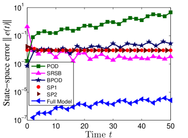
(a) The evolution of the state-space error $\|e(t)\|=\|x(t)-\hat{x}(t)\|$

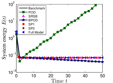
(b) The evolution of the system energy $E(t)$

Figure 1: 1D example. The evolution of the state-space error and energy for all tested methods and reduced dimension $k=4$.

First, note that POD yields the largest state and system-energy errors, and its energy grows rapidly, even within the considered time interval. This can be attributed to its eigenvalues ($\lambda=0.0828\pm 1.9679i$), which correspond to unstable modes. Because the POD reduced-order model is unstable (its matrix $\tilde{A}$ has eigenvalues with positive real parts), its infinite-time energy will be unbounded. While SRSB yields lower errors $\eta$ and $\eta_{E}$ than POD, it has larger errors over the first part of the time interval. Even though SRSB does not preserve marginal stability, its instability margin is only $2\times 10^{-4}$, which is relatively small and precludes instabilities from becoming apparent over the finite time interval considered; however, its infinite-time energy is unbounded. BPOD has smaller average errors than both POD and SRSB; however, the associated reduced-order model is asymptotically stable, which implies that its infinite-time energy is zero; thus, the reduced-order model does not have a pure marginal subsystem. Not only do the proposed SP methods produce the smallest average errors over all reduced-order models, they are also the only methods that preserve marginal stability, including the pure marginally stable subsystem. As a result, two proposed SP methods yield a finite infinite-time energy; in fact, this energy incurs a sub-1% error with respect to the infinite-time energy of the full-order model. Critically, note that extreme pure imaginary eigenvalues are exact ($\pm 2i$) in the case of SP2; this results from the fact that it balances the Hamiltonians directly.

5.2 2D mass–spring system

We now consider a 2D mass–spring system. Each mass is located on a grid point of an $(\bar{n}+2)\times(\bar{n}+2)$ grid with $\bar{n}=49$. The governing equations associated with mass $(i,j)$, $i,j=1,\ldots\bar{n}$ is given by

(57) $$m\ddot{u}_{i,j} =k_{x}(u_{i+1,j}+u_{i-1,j}-2u_{i,j})-2b\dot{u}_{i,j},$$

$$m\ddot{v}_{i,j} =k_{y}(v_{i,j+1}+v_{i,j-1}-2v_{i,j}),$$

where $u_{i,j}$ and $v_{i,j}$ are state variables representing the $x$- and $y$-displacements of mass $(i,j)$, $m=1$ denotes the mass, $k_{x}$ and $k_{y}$ denote spring constants with $k_{x}=k_{y}=2500$, and $b=1$ denotes the damping coefficient in the $x$-direction. We apply homogeneous Dirichlet boundary conditions $u_{0,j}=u_{\bar{n}+1,j}=v_{i,0}=v_{i,\bar{n}+1}=0$.

Define canonical coordinates: $q_{i,j}=u_{i,j}$, $p_{i,j}=m\dot{q}_{i,j}$, $r_{i,j}=v_{i,j}$, and $s_{i,j}=m\dot{r}_{i,j}$. The system Hamiltonian is given by $H(q_{i,j},p_{i,j},r_{i,j},s_{i,j})=H_{x}(q_{i,j},p_{i,j})+H_{y}(r_{i,j},s_{i,j})$, where

(58) $$H_{x}(q_{i,j},p_{i,j})=\frac{1}{2m}\sum_{i,j=1}^{\bar{n}}p_{i,j}^{2}+\frac{k_{x}}{2}\sum_{i,j=0}^{\bar{n}}(q_{i+1,j}-q_{i,j})^{2},$$

$$H_{y}(r_{i,j},s_{i,j})=\frac{1}{2m}\sum_{i,j=1}^{\bar{n}}s_{i,j}^{2}+\frac{k_{y}}{2}\sum_{i,j=0}^{\bar{n}}(r_{i,j+1}-r_{i,j})^{2}.$$

Now, the original system (57) can represented by dissipative Hamiltonian ordinary differential equations,

(59) $$\dot{q}_{i,j} =\frac{\partial H}{\partial p_{i,j}},\quad\quad\quad\dot{p}_{i,j}=-\frac{\partial H}{\partial q_{i,j}}-\frac{2b}{m}p_{i,j},$$

$$\dot{r}_{i,j} =\frac{\partial H}{\partial s_{i,j}},\quad\quad\quad\dot{s}_{i,j}=-\frac{\partial H}{\partial r_{i,j}}.$$

Let $q=[q_{1,1}\ \cdots\ q_{1,\bar{n}}\ \cdots\ q_{\bar{n},1}\ \cdots\ q_{\bar{n},\bar{n}}]^{\tau}$ and $r=[r_{1,1}\ \cdots\ r_{1,\bar{n}}\ \cdots\ r_{\bar{n},1}\ \cdots\ r_{\bar{n},\bar{n}}]^{\tau}$ denote the generalized coordinates. Let $p=[p_{1,1}\ \cdots\ p_{1,\bar{n}}\ \cdots\ p_{\bar{n},1}\ \cdots\ p_{\bar{n},\bar{n}}]^{\tau}$ and $s=[s_{1,1}\ \cdots\ s_{1,\bar{n}}\ \cdots\ s_{\bar{n},1}\ \cdots\ s_{\bar{n},\bar{n}}]^{\tau}$ denote the generalized momenta. With $\psi_{x}=[q^{\tau}\ p^{\tau}]^{\tau}\in\mathbb{R}^{2\bar{n}^{2}}$ and $\psi_{y}=[r^{\tau}\ s^{\tau}]^{\tau}\in\mathbb{R}^{2\bar{n}^{2}}$, the above equation can be written as matrix form, i.e.,

(60) $$\frac{d}{dt}\begin{bmatrix}\psi_{x}\\ \psi_{y}\end{bmatrix}=\begin{bmatrix}A_{s}&0\\ 0&A_{m}\\ \end{bmatrix}\begin{bmatrix}\psi_{x}\\ \psi_{y}\end{bmatrix},$$

where $\dot{\psi}_{x}=A_{s}\psi_{x}$ represents an asymptotically stable system and $\dot{\psi}_{y}=A_{m}\psi_{y}$ represents a (pure marginally stable) Hamiltonian system. Thus, the dimension of the full-order model is $n=4\bar{n}^{2}$.

Because the original system is neither controllable nor observable, SRSB cannot be directly used, as it requires solvability of Lyapunov equations (71) and (72). Instead, we compute the Gramians $M_{o}^{\mu}$ and $M_{c}^{\mu}$ by solving the modified Lyapunov equations $(A-\mu I)^{\tau}M_{o}^{\mu}+M_{o}^{\mu}(A-\mu I)=-(C^{\tau}C+\varepsilon I)$ and $(A-\mu I)M_{c}^{\mu}+M_{c}^{\mu}(A-\mu I)^{\tau}=-(BB^{\tau}+\varepsilon I)$, and let $\varepsilon=10^{-4}$. We set the shift margin to $\mu=1$.

We again test two SP methods; both of them reduce $A_{s}$ and $A_{m}$ from dimension $n/2$ to dimension $k/2$. The first SP method, SP1, is identical to the SP1 method employed in the previous example. The second SP method, SP2, applies a different balancing approach. Because the asymptotically stable subsystem is neither controllable nor observable, balanced truncation cannot be directly used for this subsystem as well. Thus, we also compute Gramians by solving the modified Lyapunov equations $A^{\tau}M_{o}+M_{o}A=-(C^{\tau}C+\varepsilon I)$ and $AM_{c}+M_{c}A^{\tau}=-(BB^{\tau}+\varepsilon I)$. For the pure marginally stable subsystem, we collect snapshot ensemble $\{\psi_{y}(i\Delta t)\}_{i=0}^{N-1}$ and construct two snapshot matrices $R=\begin{bmatrix}r_{0}\ \cdots\ r_{N-1}\end{bmatrix}$ and $S=\begin{bmatrix}s_{0}\ \cdots\ s_{N-1}\end{bmatrix}$ in $\mathbb{R}^{\bar{n}^{2}\times N}$, where $\psi_{y}(i\Delta t)=\begin{bmatrix}r_{i}^{\tau}\ s_{i}^{\tau}\end{bmatrix}^{\tau}$. Then, the symplectic balancing method (the first method in Table 5) is employed with $\Xi=RR^{\tau}$ and $\Xi^{\prime}=SS^{\tau}$. Since the pure marginally stable subsystem in this example is a standard Hamiltonian, we have $J_{\Omega}=J_{n/2}$ and $G=I_{n/2}$.

Let $\alpha(x)=\frac{|x-{l/2}|}{l/10}$ with $l=1$ the length of the spatial interval in each direction and $h(\alpha)$ be a cubic spline

$$\begin{array}[]{l}h(\alpha)=\left\{\begin{array}[]{ccl}\vspace{3pt}1-\frac{3}{2}\alpha^{2}+\frac{3}{4}\alpha^{3}&\text{if }&0\leq\alpha\leq 1,\\ \frac{1}{4}(2-\alpha)^{3}&\text{if }&1<\alpha\leq 2,\\ 0&\text{if }&\alpha>2.\end{array}\right.\end{array}$$

Let $x_{i}=il/\bar{n}$ and $y_{j}=jl/\bar{n}$. For our numerical experiments, the initial condition is provided by

(61) $$q_{i,j}(0)=r_{i,j}(0)=h(\alpha(x_{i}))h(\alpha(y_{j})),\quad\quad\quad p_{i,j}(0)=s_{i,j}(0)=0.$$

We employ a time step of $\delta t=0.002$ and set the final time to $t_{f}=15$ to compute the errors $\eta$ and $\eta_{E}$; Thus, $T=75001$. Figure 2 depicts the initial condition and final state computed by the full-order model. For the purpose of constructing basis matrices, we collect $N=101$ snapshots from the time domain $[0,5]$ with snapshot interval $\Delta t=0.05$.

(a) $q(0)$

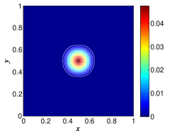
(b) $r(0)$

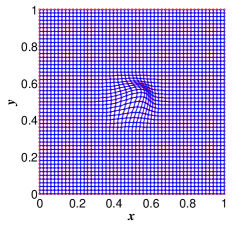
(c) Mass $(i,j)$ at $t=0$, $i,j=0,\ldots,50$

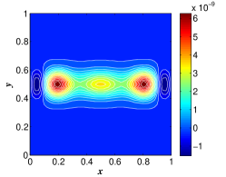
(d) $q(t_{f})$

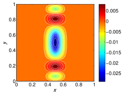
(e) $r(t_{f})$

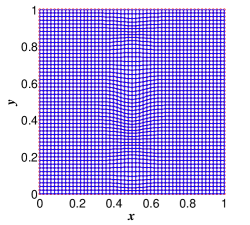
(f) Mass $(i,j)$ at $t=t_{f}$, $i,j=0,\ldots,50$

Figure 2: 2D mass–spring example. Initial condition and final state.

Table 7 compares the performance of different reduced-order models (all of dimension $k=40$), while Figure 3 plots the $\ell^{2}$-norm of the state-space error $e(t){:=}x(t)-\hat{x}(t)$ and the system energy $E(t)$ for those reduced-order models as a function of time. Here, the system energy is defined by the total Hamiltonian, i.e., $E=H(q_{i,j},p_{i,j},r_{i,j},s_{i,j})$, and its infinite-time value is computed by eigenvalue analysis.

Table 7: 2D mass–spring example. Comparison of different model-reduction methods for reduced dimension $k=40$.

	POD	SRSB	BPOD	SP1	SP2	Full-order model
Number of unstable modes	8	16	18	0	0	0
Instability margin $\max({\rm{Re}}(\lambda))$	50.480	10.586	3.695	0	0	0
Marginal-stability preservation	No	No	No	Yes	Yes	Yes
Relative state-space error $\eta$	$+\infty$	$+\infty$	$+\infty$	0.11156	0.10214	0.04358
Relative system-energy error $\eta_{E}$	$+\infty$	$+\infty$	$+\infty$	$8.6868\times 10^{-5}$	$4.8843\times 10^{-3}$	$3.413\times 10^{-5}$
Infinite-time energy	$+\infty$	$+\infty$	$+\infty$	$1.9958\times 10^{-3}$	$1.9959\times 10^{-3}$	$1.9959\times 10^{-3}$

First, note that among all the tested methods, only the full-order model and the proposed SP reduced-order models preserve marginal stability and have finite errors $\eta$ and $\eta_{E}$. Further, the SP methods ensure that the reduced-order model has a pure marginally stable subsystem, and thus a finite infinite-time energy that is nearly identical to that of the full-order model. Because POD, SRSB, and BPOD have unstable modes, they yield unbounded infinite-time energy. Further, due to their relatively large instability margins, their errors and energy grow rapidly within the considered time interval, leading to significant errors.

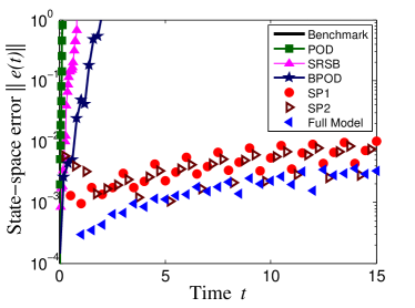
(a) The evolution of the state-space error $\|e(t)\|=\|x(t)-\hat{x}(t)\|$

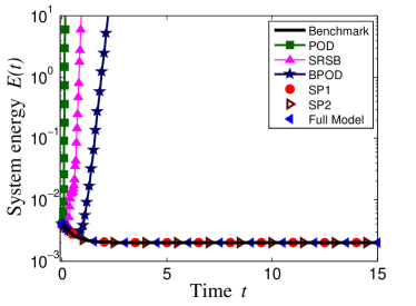
(b) The evolution of the system energy $E(t)$

Figure 3: 2D mass–spring example. The evolution of the state-space error $\|e(t)\|=\|x(t)-\hat{x}(t)\|$ and system energy $E(t)$ for all tested methods and reduced dimension $k=40$.

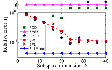
(a) Relative state-space error $\eta$ versus subspace dimension $k$

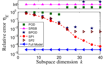
(b) Relative system-energy error $\eta_{E}$ versus subspace dimension $k$

Figure 4: 2D mass–spring example. Method performance as a function of reduced dimension $k$.

Finally, we vary the reduced dimension between $k=4$ to $k=40$ to assess the effect of subspace dimension on method performance. Figure 5.4 plots the relative state-space error $\eta$ of state variable and the relative system-energy error $\eta_{E}$ as a function of $k$. Only the full-order model and the SP reduced-order models yield finite values of $\eta$ and $\eta_{E}$ for all the tested values of subspace dimension $k$.

6 Conclusions

This work proposed a model-reduction method that preserves marginal stability for linear time-invariant (LTI) systems. The method decomposes the LTI system into asymptotically stable and pure marginally stable subsystems, and subsequently performs structure-preserving model reduction on the subsystems separately. Advantages of the method include

• its ability to preserve marginal stability,

• its ability to ensure finite infinite-time energy,

• its ability to balance primal and dual energy functionals for both subsystems.

A geometric perspective enabled a unified comparison of the proposed inner-product and symplectic projection methods.

Two numerical examples demonstrated the stability and accuracy of the proposed method. In particular, the proposed method yielded a finite infinite-time energy, while all other tested methods (i.e., POD–Galerkin, shift-reduce-shift-back, and balanced POD) produced an infinite (unstable) or zero (asymptotically stable) response.

Appendix A System decomposition in the general case

We now extend the decomposition method (in Section 2.3) to a general case where the original system is unstable and $A$ is singular. Let $T\in\mathbb{R}^{n\times n}$ be a nonsingular matrix such that a similarity transformation gives

(62) $$A=T\begin{bmatrix}A_{s}&0&0&0\\ 0&A_{m}&0&0\\ 0&0&A_{u}&0\\ 0&0&0&0\end{bmatrix}T^{-1},$$

where all eigenvalues of $A_{u}\in\mathbb{R}^{n_{u}\times n_{u}}$ have a positive real part. Substituting $x=T[x_{s}^{\tau}\ x_{m}^{\tau}\ x_{u}^{\tau}\ x_{f}^{\tau}]^{\tau}$ into (1) and premultiplying the first set of equations by $T^{-1}$ yields a decoupled LTI system

(63) $$\begin{split}\frac{d}{dt}\begin{bmatrix}x_{s}\\ x_{m}\\ x_{u}\\ x_{f}\end{bmatrix}&=\begin{bmatrix}A_{s}&0&0&0\\ 0&A_{m}&0&0\\ 0&0&A_{u}&0\\ 0&0&0&0\end{bmatrix}\begin{bmatrix}x_{s}\\ x_{m}\\ x_{u}\\ x_{f}\end{bmatrix}+\begin{bmatrix}B_{s}\\ B_{m}\\ B_{u}\\ B_{f}\end{bmatrix}u\\ y&=\begin{bmatrix}C_{s}&C_{m}&C_{u}&C_{f}\end{bmatrix}\begin{bmatrix}x_{s}\\ x_{m}\\ x_{u}\\ x_{f}\end{bmatrix},\end{split}$$

where $T^{-1}B=\begin{bmatrix}B_{s}^{\tau}&B_{m}^{\tau}&B_{u}^{\tau}&B_{f}^{\tau}\end{bmatrix}^{\tau}$ and $CT=\begin{bmatrix}C_{s}&C_{m}&C_{u}&C_{f}\end{bmatrix}$. Here, the subsystem associated with $x_{u}$ is antistable, and the subsystem associated with $x_{f}$ has $0$ as system matrix and is marginally stable.

In the general case characterized by decomposition (63), we can perform this reduction by defining biorthogonal test and trial basis matrices for each subsystem $\Psi_{i}\in\mathbb{R}_{*}^{n_{i}\times k_{i}}$, $\Phi_{i}\in\mathbb{R}_{*}^{n_{i}\times k_{i}}$, $i\in\{s,m,u,f\}$ . Applying Petrov–Galerkin projection to (63) with test basis matrix $\mathop{\operator@font diag}\nolimits(\Psi_{i})$ and trial basis matrix $\mathop{\operator@font diag}\nolimits(\Phi_{i})$ yields a decoupled reduced LTI system

(64) $$\begin{split}\frac{d}{dt}\begin{bmatrix}z_{s}\\ z_{m}\\ z_{u}\\ z_{f}\end{bmatrix}&=\begin{bmatrix}\tilde{A}_{s}&0&0&0\\ 0&\tilde{A}_{m}&0&0\\ 0&0&\tilde{A}_{u}&0\\ 0&0&0&0\end{bmatrix}\begin{bmatrix}z_{s}\\ z_{m}\\ z_{u}\\ z_{f}\end{bmatrix}+\begin{bmatrix}\tilde{B}_{s}\\ \tilde{B}_{m}\\ \tilde{B}_{u}\\ \tilde{B}_{f}\end{bmatrix}u\\ y&=\begin{bmatrix}\tilde{C}_{s}&\tilde{C}_{m}&\tilde{C}_{u}&\tilde{C}_{f}\end{bmatrix}\begin{bmatrix}z_{s}\\ z_{m}\\ z_{u}\\ z_{f}\end{bmatrix},\end{split}$$

where $\tilde{A}_{i}=\Psi_{i}^{\tau}A\Phi_{i}\in\mathbb{R}^{k_{i}\times k_{i}}$, $\tilde{B}_{i}=\Psi_{i}^{\tau}B\in\mathbb{R}^{k_{i}\times p}$, $\tilde{C}_{i}=C\Phi_{i}\in\mathbb{R}^{q\times k_{i}}$, $i\in\{s,m,u,f\}$.

The techniques proposed in this work can be employed to construct $(\Psi_{i},\Phi_{i})$, $i\in\{s,m\}$, while bases $(\Psi_{u},\Phi_{u})$ can be computed to preserve antistability in the associated reduced subsystem (e.g., via techniques proposed in Refs. [33, 51, 41]). Because $A_{f}=0$, $\tilde{A}_{f}=\Psi_{f}^{\tau}A_{f}\Phi_{f}=0$ holds for any $\Psi_{f}$ and $\Phi_{f}$. Thus, we can choose any existing method, (e.g., POD, balanced truncation, and balanced POD) and the reduced subsystem associated with $x_{f}$ always preserves pure marginal stability.

Appendix B Canonical form of Lyapunov equation

We now prove a claim at the end of Section 3.1, which states that any Hurwitz matrix can be transformed by a similarity transformation to a matrix with negative-definite symmetric part; in other words, a similarity transform enables any Hurwitz matrix to satisfy the canonical Lyapunov inequality $A_{0}^{\tau}+A_{0}\prec 0$. This is in analogue to Lemma 26, which shows that a generalized Hamiltonian matrix can be transformed into a Hamiltonian matrix that satisfies the canonical Hamiltonian property.

Lemma 41.

A Hurwitz matrix $A$ can be transformed into a matrix $A_{0}$ with negative symmetric part by similarity transformation with a real matrix $G$. Conversely, if the system matrix $A$ can be transformed into a matrix $A_{0}$ with negative symmetric part by a similarity transformation, then $A$ is a Hurwitz matrix.

Proof.

Because $A\in\mathrm{H}(n)$, there exists $\Theta\in\mathrm{SPD}(n)$ such that the Lyapunov inequality (11) holds. Choose $G\in\mathbb{R}_{*}^{n}$ (e.g., $G=\Theta^{-1/2}$) such that $G^{\tau}\Theta G=I_{n}$. Left- and right-multiplying (11) by $G^{\tau}$ and $G$, respectively, yields

$$(G^{\tau}AG^{-\tau})(G^{\tau}\Theta G)+(G^{\tau}\Theta G)(G^{-1}AG)\prec 0.$$

Let $A_{0}=G^{-1}AG$. Then, the above equation implies $A_{0}^{\tau}+A_{0}\prec 0$, i.e., $A_{0}$ has negative symmetric part.

Conversely, suppose that $A_{0}=G^{-1}AG$, where $A_{0}$ has negative symmetric part and $G$ is nonsingular. Substituting $A_{0}=G^{-1}AG$ into $A_{0}^{\tau}+A_{0}\prec 0$ yields

$$(G^{-1}AG)^{\tau}+G^{-1}AG\prec 0.$$

Left- and right-multiplying the above equation by $G^{-\tau}$ and $G^{-1}$, respectively, yields

$$A^{\tau}(G^{-\tau}G^{-1})+(G^{-\tau}G^{-1})A\prec 0.$$

Let $\Theta=G^{-\tau}G^{-1}$. Then, $\Theta\in\mathrm{SPD}(n)$ and the above equation gives (11). Thus, $A\in\mathrm{H}(n)$ by Lemma 5. ∎

Appendix C Cotangent lift

The end of Section 4.5 mentions that there is no general way to construct a trial basis matrix satisfying $\Phi\in\mathrm{Sp}(J_{\Omega},J_{\Pi})$. This section briefly reviews the cotangent lift method, which is an SVD-based method to construct $\Phi_{0}\in\mathrm{Sp}(J_{2n},J_{2k})$; from this matrix, a trial basis matrix satisfying $\Phi\in\mathrm{Sp}(J_{\Omega},J_{\Pi})$ can then be computed from Method 3 in Table 5 using $\Phi_{0}$ as an input.

The cotangent lift method [38, 37] assumes that $\Phi_{0}$ has a block diagonal form, i.e., $\Phi_{0}={\rm{diag}}(\bar{\Phi},\bar{\Phi})$ for some $\bar{\Phi}\in\mathbb{R}_{*}^{n\times k}$. Then $\Phi_{0}^{\tau}J_{2n}\Phi_{0}=J_{2k}$ holds if and only if $\bar{\Phi}^{\tau}\bar{\Phi}=I_{k}$. Thus, $\bar{\Phi}$ is orthonormal, i.e., $\bar{\Phi}\in O(I_{n},I_{k})$. Assume we have snapshots of a pure marginally stable system $\{x_{i}\}_{i=1}^{N}$; then, we apply the inverse symplectic transformation to obtain the associated snapshots in the canonical coordinates $\{y_{i}\}_{i=1}^{N}$ with $y_{i}=G^{-1}x_{i}$, $i=1,\ldots,N$. Writing the decomposition $y_{i}=\begin{bmatrix}q_{i}^{\tau}\ p_{i}^{\tau}\end{bmatrix}^{\tau}\in\mathbb{R}^{2n}$ with $q_{i},p_{i}\in\mathbb{R}^{n}$, $\bar{\Phi}$ can be computed by the SVD of an extended snapshot matrix $M_{\rm{cot}}=\begin{bmatrix}q_{1}\cdots q_{N}\ p_{1}\cdots p_{N}\end{bmatrix}\in\mathbb{R}^{n\times 2N}$.

Algorithm 3 Cotangent lift

0:  Snapshots $\{x_{i}\}_{i=1}^{N}\subset\mathbb{R}^{2n}$ with and a symplectic transformation matrix $G$ associated with a pure marginally stable system.

0:  A symplectic matrix $\Phi_{0}\in\mathrm{Sp}(J_{2n},J_{2k})$ in block-diagonal form.

1:  Apply inverse symplectic transformation to snapshots $y_{i}=G^{-1}x_{i}$, $i=1,\ldots,N$.

2:  Form the extended snapshot matrix $M_{\rm{cot}}=\begin{bmatrix}q_{1}\cdots\ q_{N}\ p_{1}\cdots\ p_{N}\end{bmatrix}$, where $y_{i}=\begin{bmatrix}q_{i}^{\tau}\ p_{i}^{\tau}\end{bmatrix}^{\tau}$.

3:  Compute the SVD of $M_{\rm{cot}}$; the basis matrix $\bar{\Phi}$ comprises the first $k$ left singular vectors of $M_{\rm{cot}}$.

4:  Construct the symplectic matrix $\Phi_{0}={\rm{diag}}(\bar{\Phi},\bar{\Phi})$.

Algorithm 3 lists the detailed procedure of the cotangent lift. Although the cotangent lift method can only find a near optimal solution to fit empirical data, we can prove that the projection error of cotangent lift is no greater than the projection error of POD with a constant factor [37].

Appendix D Generalized system energy

If the original system is asymptotically stable, we can define a quadratic function as the system energy [43]. When it is marginally stable, we can extend the definition; the system energy is used in Section 5.1 to measure the performance of several model reduction methods. Suppose the matrix $\Theta=M\in\mathrm{SPD}(n_{s})$ satisfies the Lyapunov equation (4) for the asymptotically stable subsystem. Suppose $H:x_{m}\mapsto{\frac{1}{2}}{x_{m}^{\tau}}Lx_{m}$ is the Hamiltonian function of the marginally stable subsystem with $L\in\mathrm{SPD}(n_{m})$. With $(x_{s}^{\tau},x_{m}^{\tau})^{\tau}=T^{-1}x$, the system energy can be defined as

(65) $$E(t)={\frac{1}{2}}{\begin{bmatrix}x_{s}(t)^{\tau}&x_{m}(t)^{\tau}\end{bmatrix}}\begin{bmatrix}M&0\\ 0&L\end{bmatrix}{\begin{bmatrix}x_{s}(t)\\ x_{m}(t)\end{bmatrix}}=\frac{1}{2}\|x_{s}(t)\|_{M}^{2}+H(x_{m}(t)),$$

The time evolution of the system energy is given by

$$\frac{d}{dt}E(t) =\frac{1}{2}(\dot{x}_{s}^{\tau}Mx_{s}+x_{s}^{\tau}M\dot{x}_{s})+\frac{1}{2}(\dot{x}_{m}^{\tau}Lx_{m}+x_{m}^{\tau}L\dot{x}_{m})=\frac{1}{2}x_{s}^{\tau}(A_{s}^{\tau}M+MA_{s})x_{s}+\frac{1}{2}x_{m}^{\tau}(A_{m}^{\tau}L+LA_{m})x_{m}$$

$$=-\frac{1}{2}x_{s}^{\tau}Qx_{s}+\frac{1}{2}x_{m}^{\tau}(-LJL+LJL)x_{m}=-\frac{1}{2}x_{s}^{\tau}Qx_{s}.$$

In the third equality, we use the Lyaponuv equation $A_{s}^{\tau}M+MA_{s}=-Q$, the definition $A_{m}=JL$, and the fact that $J$ is skew-symmetric. Because $Q\in\mathrm{SPD}(n_{s})$, the system energy is strictly decreasing in time when $x_{s}\neq 0$.

Appendix E Review of existing model reduction methods

In this section, we briefly review a few existing model reduction methods, including POD–Galerkin (POD), balanced truncation, balanced POD, and shift-reduce-shift-back (SRSB), as listed in Table 8. Section 5 numerically compares the performance of these methods with the proposed structure-preserving technique. We show that each of these methods exhibits an inner-product structure (see Table 3 in Section 3.5); however, the associated inner-product matrix $M$ does not associate with a Lyapunov matrix in all cases, which precludes some methods from ensuring asymptotic-stability preservation.

Table 8: Algorithms for computing test and trial basis matrices using existing model-reduction methods

	POD–Galerkin	Balanced truncation	Balanced POD	SRSB
Input	Snapshots $X$ in (66)	$(A,B,C)$	Primal snapshots $S$ in (69) Dual snapshots $R$ in (70)	$(A,B,C)$ Shift margin $\mu$
Output	$\Psi$, $\Phi\in O(I_{n},I_{k})$.	$\Phi\in O(W_{o},\Sigma_{1})$, $\Psi\in O(W_{c},\Sigma_{1})$	$\Phi\in O(\hat{W}_{o},\Sigma_{1})$; $\Psi\in O(\hat{W}_{c},\Sigma_{1})$.	$\Phi\in O(W_{o}^{\mu},\Sigma_{1})$, $\Psi\in O(W_{c}^{\mu},\Sigma_{1})$
Algorithm	1. Compute SVD     $X=U\Sigma V^{\tau}$. 2. $\Psi=\Phi=U_{1}$.	1. Compute $W_{o}$ by (67) 2. Compute $W_{c}$ by (68). 3. Compute symmetric factorization     $W_{c}=SS^{\tau}$, $W_{o}=RR^{\tau}$. 4. Compute SVD     $R^{\tau}S=U\Sigma V^{\tau}$. 5. $\Phi=SV_{1}\Sigma_{1}^{-1/2}$. 6. $\Psi=RU_{1}\Sigma_{1}^{-1/2}$.	1. Compute SVD     $R^{\tau}S=U\Sigma V^{\tau}$ 2. $\Phi=SV_{1}\Sigma_{1}^{-1/2}$ 3. $\Psi=RU_{1}\Sigma_{1}^{-1/2}$.	1. Compute $W_{o}^{\mu}$ by (71) 2. Compute $W_{c}^{\mu}$ by (72). 3. Compute symmetric factorization     $W_{c}^{\mu}=SS^{\tau}$, $W_{o}^{\mu}=RR^{\tau}$. 4. Compute SVD     $R^{\tau}S=U\Sigma V^{\tau}$. 5. $\Phi=SV_{1}\Sigma_{1}^{-1/2}$. 6. $\Psi=RU_{1}\Sigma_{1}^{-1/2}$.

E.1 POD–Galerkin

POD [24] computes a basis $\Phi$ that minimizes the mean-squared projection error of a set of snapshots $\{x_{i}\}_{i=1}^{N}$, i.e., satisfies optimality property (26) with $M=I_{n}$ and $N=I_{k}$. Algebraically, POD computes the singular value decomposition (SVD)

(66) $$X=\begin{bmatrix}x_{1}&\cdots&x_{N}\end{bmatrix}=U\Sigma V^{\tau},$$

where $U\in O(I_{n},I_{r})$, $\Sigma=\mathop{\operator@font diag}\nolimits(\sigma_{1},\ldots,\sigma_{r})$ with singular values $\sigma_{1}\geq...\geq\sigma_{r}\geq 0$, $V\in O(I_{N},I_{r})$, and $r=\min(n,N)$. Then, both the trial and test basis matrices are set to the first $k$ columns of $U$, which is equivalent to enforcing the Galerkin orthogonality condition (i.e., performing Galerkin projection).

As reported in Table 3, it can be verified that POD–Galerkin corresponds to an inner-product balancing with $\Xi=\Xi^{\prime}=XX^{\tau}$. Thus, $\Psi,\Phi\in O(XX^{T},\Sigma^{2})$; however, note that we also have $\Psi,\Phi\in O(I_{n},I_{k})$.

E.2 Balanced truncation

Balanced truncation [34] can be applied to LTI systems that are asymptotically stable, controllable, and observable. In the present framework, balanced truncation corresponds to a specific type of inner-product balancing with $\Xi=W_{o}$ and $\Xi^{\prime}=W_{c}$, where $W_{o}$ and $W_{c}$ represent observability and controllability Gramians that satisfy primal and dual Lyapunov equations

(67) $$A^{\tau}W_{o}+W_{o}A =-C^{\tau}C,$$

(68) $$AW_{c}+W_{c}A^{\tau} =-BB^{\tau},$$

respectively, which are defined for observable and controllable asymptotically stable LTI systems. While the present framework cannot prove that balanced truncation preserves asymptotic stability (the right-hand-side matrices in the Lyapunov equations (67)–(68) are positive semidefinite), it can be shown using observable and controllable conditions that balanced truncation does in fact preserve asymptotic stability [3, pp. 213–215].

E.3 Balanced POD

Several techniques exist to solve the Lyapunov equations (67) and (68) for the controllability and observability Gramians [3]; however, they are prohibitively expensive for large-scale systems. For this reason, several methods have been developed that instead employ empirical Gramians [lall2002sab] that approximate the analytical Gramians. One particular method is balanced POD (BPOD) [47, 42], which relies on collecting primal snapshots for $N$ time steps (one impulse response of the forward system per column in $B$):

(69) $$S=\begin{bmatrix}B&e^{A\Delta t}B&\cdots&e^{A(N-1)\Delta t}B\end{bmatrix}$$

and dual snapshots for $N$ time steps (one impulse response of the dual system per row in $C$):

(70) $$R=\begin{bmatrix}C^{\tau}&e^{A^{\tau}\Delta t}C^{\tau}&\cdots&e^{A^{\tau}(N-1)\Delta t}C^{\tau}\end{bmatrix};$$

the empirical observability and controllability Gramians are then set to $\hat{W}_{o}=RR^{\tau}$ and $\hat{W}_{c}=SS^{\tau}$, respectively. Then, BPOD corresponds to inner-product balancing with $\Xi=\hat{W}_{o}$ and $\Xi^{\prime}=\hat{W}_{c}$.

Critically, empirical Gramians $\hat{W}_{o}$ and $\hat{W}_{c}$ may not be Lyapunov matrices, i.e., they may not satisfy (11) and (13), respectively. Consequently, unlike balanced truncation, balanced POD does not guarantee asymptotic-stability preservation.

E.4 SRSB

The shift-reduce-shift-back (SRSB) method aims to extend the applicability of balanced truncation to marginally stable and unstable systems [50, 8, 44, 52, 49].

By Lemma 5, the real parts of the eigenvalues of $A$ are less than the shift margin $\mu\in\mathbb{R}$ if and only if given any $Q\in\mathrm{SPD}(n)$, there exists $\Theta\in\mathrm{SPD}(n)$ that is the unique solution to

$$(A-\mu I)^{\tau}\Theta+\Theta(A-\mu I)=-Q.$$

Thus, even if $A$ is marginally stable or unstable, we can choose $\mu$ such that the shifted system corresponding to the matrix $A-\mu I$ is asymptotically stable and the test and trial basis matrices can be computed by performing balanced truncation on the shifted system. The basis matrices can be applied to the original (unshifted) system. Table 8 provides the associated algorithm, which amounts to computing an inner-product balancing with $\Xi=W_{o}^{\mu}$ and $\Xi^{\prime}=W_{c}^{\mu}$, where the shifted observability and controllability Gramians satisfy

(71) $$(A-\mu I)^{\tau}W_{o}^{\mu}+W_{o}^{\mu}(A-\mu I) =-C^{\tau}C,$$

(72) $$(A-\mu I)W_{c}^{\mu}+W_{c}^{\mu}(A-\mu I)^{\tau} =-BB^{\tau}.$$

While SRSB ensures that the shifted reduced system $(\Psi^{\tau}(A-\mu I_{n})\Phi,\Psi^{\tau}B,C\Phi)=(\tilde{A}-\mu I_{k},\tilde{B},\tilde{C})$ remains asymptotically stable, this guarantee does not extend to the reduced system $(\tilde{A},\tilde{B},\tilde{C})$ that is used in practice. In particular, there is no assurance that the reduced system will retain the asymptotic or marginal stability that characterized the original system $(A,B,C)$.

References

• [1] B. M. Afkham and J. S. Hesthaven, Structure preserving model reduction of parametric Hamiltonian systems, (2017). http://arXiv:1703.08345.
• [2] D. Amsallem and C. Farhat, Stabilization of projection-based reduced-order models, Int. J. Numer. Meth. Eng., 91 (2012), pp. 358–377.
• [3] A. C. Antoulas, Approximation of Large-Scale Dynamical Systems, SIAM, Philadelphia, PA, 2005.
• [4] N. Aubry, P. Holmes, J. L. Lumley, and E. Stone, The dynamics of coherent structures in the wall region of a turbulent boundary layer, J. Fluid Mech., 192 (1988), pp. 115–173.
• [5] Z. Bai, Krylov subspace techniques for reduced-order modeling of large-scale dynamical systems, Appl. Numer. Math., 43 (2002), pp. 9–44.
• [6] M. Balajewicz, I. Tezaur, and E. Dowell, Minimal subspace rotation on the Stiefel manifold for stabilization and enhancement of projection-based reduced order models for the compressible Navier–Stokes equations, J. Comput. Phys., 321 (2016), pp. 224–241.
• [7] M. J. Balajewicz, E. H. Dowell, and B. R. Noack, Low-dimensional modeling of high-Reynolds-number shear flows incorporating constraints from the Navier-Stokes equation, J. Fluid Mech., 729 (2013), pp. 285–308.
• [8] M. Barahona, A. C. Doherty, M. Sznaier, H. Mabuchi, and J. C. Doyle, Finite horizon model reduction and the appearance of dissipation in Hamiltonian systems, in Proceedings of the 41st IEEE Conference on Decision and Control, Las Vegas, NV, December 2002, pp. 4563–4568.
• [9] M. F. Barone, I. Kalashnikova, D. J. Segalman, and H. K. Thornquist, Stable Galerkin reduced order models for linearized compressible flow, J. Comput. Phys., 228 (2009), pp. 1932–1946.
• [10] M. Bergmann, C.-H. Bruneau, and A. Iollo, Enablers for robust POD models, J. Comput. Phys., 228 (2009), pp. 516–538.
• [11] B. N. Bond and L. Daniel, Guaranteed stable projection-based model reduction for indefinite and unstable linear systems, in Proceedings of the 2008 IEEE/ACM International Conference on Computer-Aided Design, San Jose, CA, November 2008, pp. 728–735.
• [12] K. Carlberg, R. Tuminaro, and P. Boggs, Efficient structure-preserving model reduction for nonlinear mechanical systems with application to structural dynamics, AIAA paper 2012-1969, 53rd AIAA/ASME/ASCE/AHS/ASC Structures, Structural Dynamics and Materials Conference, Honolulu, HI, April 2012.
• [13]  , Preserving Lagrangian structure in nonlinear model reduction with application to structural dynamics, SIAM J. Sci. Comput., 37 (2015), pp. B153–B184.
• [14] W. Cazemier, R. W. C. P. Verstappen, and A. E. P. Veldman, Proper orthogonal decomposition and low-dimensional models for driven cavity flows, Phys. Fluids, 10 (1998), pp. 1685–1699.
• [15] M. Couplet, C. Basdevant, and P. Sagaut, Calibrated reduced-order POD-Galerkin system for fluid flow modelling, J. Comput. Phys., 207 (2005), pp. 192–220.
• [16] J. Delville, L. Ukeiley, L. Cordier, J. P. Bonnet, and M. Glauser, Examination of large-scale structures in a turbulent plane mixing layer. Part 1. Proper orthogonal decomposition, J. Fluid Mech., 391 (1999), pp. 91–122.
• [17] H. Eves, Elementary Matrix Theory, Dover, New York, 1980.
• [18] R. W. Freund, Model reduction methods based on Krylov subspaces, Acta Numerica, 12 (2003), pp. 267–319.
• [19] K. Glover, All optimal Hankel-norm approximations of linear mutilvariable systems and their $L^{\infty}$-error bounds, Int. J. Control, 39 (1984), pp. 1115–1193.
• [20] S. Gugercin, A. C. Antoulas, and C. Beattie, $\mathcal{H}_{2}$ model reduction for large-scale linear dynamical systems, SIAM. J. Matrix Anal. Appl., 30 (2008), pp. 609–638.
• [21] S. Gugercin, R. V. Polyuga, C. Beattie, and A. van der Schaft, Structure-preserving tangential interpolation for model reduction of port-Hamiltonian systems, Automatica, 48 (2012), pp. 1963–1974.
• [22] C. Hartmann, V.-M. Vulcanov, and C. Schütte, Balanced truncation of linear second-order systems: A Hamiltonian approach, SIAM J. Multiscale Model. and Simul., 8 (2010), pp. 1348–1367.
• [23] J. P. Hespanha, Linear systems theory, Princeton University Press, 2009.
• [24] P. Holmes, J. L. Lumley, G. Berkooz, and C. W. Rowley, Turbulence, Coherent Structures, Dynamical Systems and Symmetry, 2nd ed., Cambridge University Press, Cambridge, UK, 2012.
• [25] I. Kalashnikova and M. F. Barone, On the stability and convergence of a Galerkin reduced order model (ROM) of compressible flow with solid wall and far-field boundary treatment, Int. J. Numer. Meth. Engng, 83 (2010), pp. 1345–1375.
• [26] I. Kalashnikova, B. van Bloemen Waanders, S. Arunajatesan, and M. Barone, Stabilization of projection-based reduced order models for linear time-invariant systems via optimization-based eigenvalue reassignment, Comput. Methods in Appl. Mech. Eng., 272 (2014), pp. 251–270.
• [27] V. L. Kalb and A. E. Deane, An intrinsic stabilization scheme for proper orthogonal decomposition based low-dimensional models, Phys. Fluids, 19 (2007), pp. 054106:1–19.
• [28] S. Lall, P. Krysl, and J. E. Marsden, Structure-preserving model reduction for mechanical systems, Phys. D, 184 (2003), pp. 304–318.
• [29] S. Lall, J. E. Marsden, and S. Glavas̆ki, A subspace approach to balanced truncation for model reduction of nonlinear control systems, Int. J. Robust Nonlin. Contr., 12 (2002), pp. 519–535.
• [30] Z. Ma, S. Ahuja, and C. W. Rowley, Reduced-order models for control of fluids using the eigensystem realization algorithm, Theor. Comput. Fluid Dyn., 25 (2011), pp. 233–247.
• [31] C. Magruder, C. Beattie, and S. Gugercin, Rational Krylov methods for optimal $\mathcal{L}_{2}$ model reduction, in 49th IEEE Conference on Decision and Control, Atlanta, GA, USA, December 2010, pp. 6797–6802.
• [32] L. Meier and D. Luenberger, Approximation of linear constant systems, IEE. Trans. Automat. Contr., 12 (1967), pp. 585–588.
• [33] N. Mirnateghi and E. Mirnateghi, Model reduction of unstable systems using balanced truncation, in IEEE 3rd International Conference on System Engineering and Technology, Shah Alam, Malaysia, August 2013, pp. 193–196.
• [34] B. C. Moore, Principal component analysis in linear systems: Controllability, observability, and model reduction, IEEE Trans. Automat. Control, 26 (1981), pp. 17–32.
• [35] B. R. Noack, K. Afanasiev, M. Morzyński, G. Tadmor, and F. Thiele, A hierarchy of low-dimensional models for the transient and post-transient cylinder wake, J. Fluid Mech., 497 (2003), pp. 335–363.
• [36] A. C. Or and J. L. Speyer, Empirical pseudo-balanced model reduction and feedback control of weakly nonlinear convection patterns, J. Fluid Mech., 662 (2010), pp. 36–65.
• [37] L. Peng and K. Mohseni, Structure-preserving model reduction of forced Hamiltonian systems, (2016). http://arXiv:1603.03514.
• [38]  , Symplectic model reduction of Hamiltonian systems, SIAM J. Sci. Comput., 38 (2016), pp. A1–A27.
• [39] B. Podvin and J. Lumley, A low-dimensional approach for the minimal flow unit, J. Fluid Mech., 362 (1998), pp. 121–155.
• [40] R. V. Polyuga and A. van der Schaft, Structure preserving model reduction of port-Hamiltonian systems by moment matching at infinity, Automatica, 46 (2010), pp. 665–672.
• [41] R. Prakash and S. V. Rao, A balancing method for reduced order modelling of unstable systems, Math. Comput. Model., 14 (1990), pp. 418–423.
• [42] C. W. Rowley, Model reduction for fluids, using balanced proper orthogonal decomposition, Int. J. on Bifurcation and Chaos, 15 (2005), pp. 997–1013.
• [43] C. W. Rowley, T. Colonius, and R. M. Murray, Model reduction for compressible flows using POD and Galerkin projection, Phys. D, 189 (2004), pp. 115–129.
• [44] J. M. Santiago and M. Jamshidi, Some extensions of the open-loop balanced approach for model reduction, in Proceedings of the American Control Conference, Boston, MA, June 1985, pp. 1005–1009.
• [45] G. Serre, P. Lafon, X. Gloerfelt, and C. Bailly, Reliable reduced-order models for time-dependent linearized Euler equations, J. Comput. Phys., 231 (2012), pp. 5176–5194.
• [46] A. J. van der Schaft and J. E. Oeloff, Model reduction of linear conservative mechanical systems, IEEE Trans. Automat. Control, (1990), pp. 729–733.
• [47] K. Willcox and J. Peraire, Balanced model reduction via the proper orthogonal decomposition, AIAA Journal, 40 (2002), pp. 2323–2330.
• [48] D. A. Wilson, Optimum solution of model-reduction problem, in Proceedings of the Institution of Electrical Engineers, June 1970, pp. 1161–1165.
• [49] J. Yang, C. S. Chen, J. A. D. Abreu-García, and Y. Xu, Model reduction of unstable systems, Int. J. Syst. Sci., 24 (1993), pp. 2407–2414.
• [50] J. Yang, Y. Xu, and C. S. Chen, Model reduction of flexible manipulators, Tech. Rep. CMU-RI-TR-92-08, Robotics Institute, Carnegie Mellon University, June 1992.
• [51] K. Zhou, G. Salomon, and E. Wu, Balanced realization and model reduction for unstable systems, Internat. J. Robust Nonlinear Control, 9 (1999), pp. 183–198.
• [52] A. Zilouchian, Balanced structures and model reduction of unstable systems, in IEEE Proceedings of Southeastcon ’91, vol. 2, April 1991, pp. 1198–1201.