Matroid Theory and Storage Codes: Bounds and Constructions

Abstract

Recent research on distributed storage systems (DSSs) has revealed interesting connections between matroid theory and locally repairable codes (LRCs). The goal of this chapter is to introduce the reader to matroids and polymatroids, and illustrate their relation to distributed storage systems. While many of the results are rather technical in nature, effort is made to increase accessibility via simple examples. The chapter embeds all the essential features of LRCs, namely locality, availability, and hierarchy alongside with related generalised Singleton bounds.

1 Introduction to Locally Repairable Codes

In this chapter, we will discuss the theoretical foundations of locally repairable codes (LRCs), which were introduced in Chapter 14. While our main interest is in the codes and their applicability for distributed storage systems, significant parts of our machinery comes from matroid theory. We will develop this theory to the extent that is needed for the applications, and leave some additional pointers to interpretations in terms of graphs and projective geometries.

The need for large-scale data storage is continuously increasing. Within the past few years, distributed storage systems (DSSs) have revolutionised our traditional ways of storing, securing, and accessing data. Storage node failure is a frequent obstacle in large-scale DSSs, making repair efficiency an important objective. A bottle-neck for repair efficiency, measured by the notion of locality papailiopoulos12 , is the number of contacted nodes needed for repair. The key objects of study in this paper are locally repairable codes (LRCs), which are, informally speaking, storage systems where a small number of failing nodes can be recovered by boundedly many other (close-by) nodes. Repair-efficient LRCs are already in use for large-scale DSSs used by, for example, Facebook and Windows Azure Storage tamo13 .

Another desired attribute, measured by the notion of availability rawat14 , is the property of having multiple alternative ways to repair nodes or access files. This is particularly relevant for nodes containing so-called hot data that is frequently and simultaneously accessed by many users. Moreover, as failures are often spatially correlated, it is valuable to have each node repairable at several different scales. This means that if a node fails simultaneously with the set of nodes that should normally be used for repairing it, then there still exists a larger set of helper nodes that can be used to recover the lost data. This property is captured by the notion of hierarchy sasidharan15 ; izs16 in the storage system.

Network coding techniques for large-scale DSSs were considered in dimakis10 . Since then, a plethora of research on DSSs with a focus on linear LRCs and various localities has been carried out, see gopalan12 ; papailiopoulos12 ; prakash12 ; silberstein13 ; tamo14 among many others. Availability for linear LRCs was defined in rawat14 . The notion of hierarchical locality was first studied in sasidharan15 , where bounds for the global minimum distance were also obtained.

Let us denote by $(n,k,d,r,\delta,t)$, respectively, the code length, dimension, global minimum distance, locality, local minimum distance, and availability. Bold-faced parameters $(\mathbf{n},\mathbf{k},\mathbf{d},\mathbf{t})$ will be used in the sequel to refer to hierarchical locality and availability. It was shown in tamo13 that the $(r,\delta=2)$-locality of a linear LRC is a matroid invariant. The connection between matroid theory and linear LRCs was examined in more detail in westerback15 . In addition, the parameters $(n,k,d,r,\delta)$ for linear LRCs were generalised to matroids, and new results for both matroids and linear LRCs were given therein. Even more generally, the parameters $(n,k,d,r,\delta,t)$ were generalised to polymatroids, and new results for polymatroids, matroids and both linear and nonlinear LRCs over arbitrary finite alphabets were derived in polymatroid . Similar methods can be used to bound parameters of batch codes ZSbatchbound , as discussed in Chapter 16. For more background on batch codes, see e.g. IKOSbatchfirst ; LSbatchorig . Moreover, as certain specific LRCs and batch codes belong to the class of private information retrieval (PIR) codes as defined in (FVY_PIR, , Def. 4), the related LRC and batch code bounds also hold for those PIR codes. See Section 5.3 and Chapter 16 for more discussion.

The main purpose of this chapter is to give an overview of the connection between matroid theory and linear LRCs with availability and hierarchy, using examples for improved clarity of the technical results. In particular, we are focusing on how the parameters of a LRC can be analysed using the lattice of cyclic flats of an associated matroid, and on a construction derived from matroid theory that provides us with linear LRCs. The matroidal results on LRCs reviewed here are mostly taken from westerback15 ; polymatroid ; izs16 .

The rest of this chapter is organised as follows. In Sections 1.1–1.2, we introduce distributed storage systems and how they can be constructed by using linear codes. In particular, we consider locally repairable codes with availability. Section 2 gives a brief introduction to the concepts and features related to matroids relevant to LRCs. In Section 3, we summarise the state-of-the-art generalised Singleton bounds on the code parameters for linear codes, as well as discuss existence of Singleton-optimal linear codes and matroids. Section 4 reviews some explicit (linear) code constructions. In Section 5, we go beyond linear codes and consider polymatroids and related generalised Singleton bounds, which are then valid for all LRCs over any finite alphabet, and also imply bounds for PIR codes when restricted to systematic linear codes. Section 6 concludes the chapter and discusses some open problems. Further results in matroid theory and especially their representability are given in Appendix for the interested reader. The following notation will be used throughout the paper:

$\mathbb{F}$ :	a field;
$\mathbb{F}_{q}$ :	the finite field of prime power size $q$;
$E$ :	a finite set;
$G$ :	a matrix over $\mathbb{F}$ with columns indexed by $E$;
$G(X)$ :	the matrix obtained from $G$ by restricting to the
	columns indexed by $X$, where $X\subseteq E$;
$\mathrm{C}(G)$ :	the vector space generated by the columns of $G$;
$\mathrm{R}({G})$ :	the vector space generated by the rows of $G$;
$C$ :	linear code $C=\mathrm{R}({G})$ over $\mathbb{F}$ generated by $G$;
$C_{X}$ :	the punctured code of $C$ on $X$, i.e.,
	$C_{X}=\mathrm{R}({G(X)})$, where $X\subseteq E$;
$2^{E}$ :	the collection of all subsets of a finite set $E$;
$[j]$ :	the set $\{1,2,\ldots,j\}$ for a positive integer $j$;
$n,k,d,r,\delta,t,h$ :	code length, dimension, minimum distance, locality,
	failure tolerance, availability, hierarchy, respectively;
$[n,k,d]\,,(n,k,d)$ :	parameters of a linear/general code, respectively;
$(n,k,\ldots)_{i}$ :	parameter values when we consider information
	symbols, e.g., information symbol locality;
$(n,k,\ldots)_{a}$ :	parameter values when we consider all code
	symbols, e.g., all symbol locality;
$(n,k,\ldots)_{s}$ :	parameter values when we consider systematic code
	symbols, e.g., systematic symbol locality;
$(\mathbf{n},\mathbf{k},\mathbf{d},\mathbf{t})$ :	parameter values for different hierarchy levels.

Remark 1

Here, $d$ denotes the minimum (Hamming) distance of the code, rather than the number of nodes that have to be contacted for repair, as is commonplace in the theory of regenerating codes. In Chapter 14, the minimum distance of the code was denoted by $d_{H}$.

The motivation to study punctured codes arises from hierarchical locality; the locality parameters at the different hierarchy levels correspond to the global parameters of the related punctured codes. The puncturing operation on codes corresponds to the so-called restriction (or deletion) operation on matroids.

We also point out that $G(E)=G$ and $C_{E}=C$. We will often index a matrix $G$ by $[n]$, where $n$ is the number of columns in $G$.

1.1 Distributed Storage Systems from Linear Codes

A linear code $C$ can be used to obtain a DSS, where every coordinate in $C$ represents a storage node in the DSS, and every point in $C$ represents a stored data item. While one often assumes that the data items are field elements in their own right, no such assumption is necessary. However, if $C$ is a code over the field $\mathbb{F}$ and the data items are elements in an alphabet $\mathbb{A}$, then we must be able to form the linear combinations $f_{1}a_{1}+f_{2}a_{2}$ for $f_{1},f_{2}$ in $\mathbb{F}$ and $a_{1},a_{2}$ in $\mathbb{A}$. Moreover, if we know the scalar $f$, we must be able to read off $a$ from $fa$. This is achieved if $\mathbb{A}\cong\mathbb{F}^{\alpha}$ is a vector space over $\mathbb{F}$, wherefore we must have $|\mathbb{A}|\geq|\mathbb{F}|$. Thus, the length of the data items must be at least the number of symbols needed to represent a field element. In particular if the data items are measured in, e.g., kilobytes, then we are restricted to work over fields of size not larger than about $2^{8000}$. Beside this strict upper bound on the field size, the complexity of operations also makes small field sizes — ideally even binary fields — naturally desirable.

Example 1

Let $C$ be the linear code generated by the following matrix $G$ over $\mathbb{F}_{3}$:

$$\small G=\begin{tabular}[]{ |c|c|c|c|c|c|c|c|c| }\lx@intercol\hfil 1\hfil\lx@intercol&\lx@intercol\hfil 2\hfil\lx@intercol&\lx@intercol\hfil 3\hfil\lx@intercol&\lx@intercol\hfil 4\hfil\lx@intercol&\lx@intercol\hfil 5\hfil\lx@intercol&\lx@intercol\hfil 6\hfil\lx@intercol&\lx@intercol\hfil 7\hfil\lx@intercol&\lx@intercol\hfil 8\hfil\lx@intercol&\lx@intercol\hfil 9\hfil\lx@intercol\\ \hline\cr 1&0&0&0&1&1&1&1&1\\ \hline\cr 0&1&0&0&1&0&1&2&2\\ \hline\cr 0&0&1&0&0&1&1&0&0\\ \hline\cr 0&0&0&1&0&0&0&1&2\\ \hline\cr\end{tabular}$$

Then, $C$ corresponds to a $9$ node storage system, storing four files $(a,b,c,d)$, each of which is an element in $\mathbb{F}_{3}^{\alpha}$. In this system, node $1$ stores $a$, node $5$ stores $a+b$, node $9$ stores $a+2b+2d$, and so on.

Two very basic properties of any DSS are that every node can be repaired by some other nodes and that every node contains some information. We therefore give the following definition.

Definition 1

A linear $[n,k,d]$-code $C$ over a field is a non-degenerate storage code if $d\geq 2$ and there is no zero column in a generator matrix of $C$.

The first example of a storage code, and the motivating example behind the notion of locality, is the notion of a maximum distance separable (MDS) code. It has several different definitions in the literature, here we list a few of them.

Definition 2

The following properties are equivalent for linear $[n,k,d]$ storage codes:

1. $n=k+d-1$.

2. The stored data can be retrieved from any $k$ nodes in the storage system.

3. To repair any single erased node in the storage system, one needs to contact $k$ other nodes.

A code that satisfies one (and therefore all) of the above properties is called an $MDS$ code.

By the Singleton bound, $n\geq k+d-1$ holds for any storage code, so by property (i), MDS codes are “optimal” in the sense that they have minimal length for given storage capacity and error tolerance. However, (iii) is clearly an unfavourable property in terms of erasure correction. This is the motivation behind constructing codes with small $n-k-d$, where individual node failures can still be corrected “locally”.

1.2 Linear Locally Repairable Codes with Availability

The very broad class of linear LRCs will be defined next. It is worth noting that, contrary to what the terminology would suggest, a LRC is not a novel kind of code, but rather the “locality parameters” $(r,\delta)$ can be defined for any code. What we call a LRC is then only a code that is specifically designed with the parameters $(r,\delta)$ in mind. While the locality parameters can be understood directly in terms of the storage system, it is more instructive from a coding theoretic point of view to understand them via punctured codes. Then, the punctured codes will correspond exactly to the restrictions to “locality sets”, which can be used to locally repair a small number of node failures within the locality set.

Definition 3

Let $G$ be a matrix over $\mathbb{F}$ indexed by $E$ and $C$ the linear code generated by $G$. Then, for $X\subseteq E$, $C_{X}$ is a linear $[n_{X},k_{X},d_{X}]$-code where

$$\begin{array}[]{l}n_{X}=|X|,\\ k_{X}=\mathrm{rank}(G(X)),\\ d_{X}=\min\{|Y|:Y\subseteq X\hbox{ and }k_{X\setminus Y}<k_{X}\}.\end{array}$$

Alternatively, one can define the minimum distance $d_{X}$ as the smallest support of a non-zero codeword in $C_{X}=\mathrm{R}({G(X)})$. We use Definition 3, as it has the advantage of not depending on the linearity of the code.

Example 2

Consider the storage code $C$ from Example 1. Let $Y_{1}=\{1,2,3,5,6,7\}$, $X_{1}=\{1,2,5\}$ and $X_{2}=\{2,6,7\}$. Then $C_{Y_{1}}$, $C_{X_{1}}$ and $C_{X_{2}}$ are storage codes with

$$\begin{array}[]{lcl}[n_{Y_{1}},k_{Y_{1}},d_{Y_{1}}]&=&[6,3,3]\,,\\ [n_{X_{1}},k_{X_{1}},d_{X_{1}}]&=&[3,2,2]\,,\\ [n_{X_{2}},k_{X_{2}},d_{X_{2}}]&=&[3,2,2]\,.\end{array}$$

The parameter $d_{X}$ is the minimum (Hamming) distance of $C_{X}$. We say that $C$ is an $[n,k,d]$-code with $[n,k,d]=[n_{E},k_{E},d_{E}]$.

We choose the following definition for general $(n,k,d,r,\delta,t)$-LRCs (i.e., both linear and nonlinear), which we will compare to known results for linear LRCs.

Definition 4

An $(n,k,d)$-code $C$ over $A$ is a nonempty subset $C$ of $A^{n}$, where $A$ is a finite set of size $s$, $k=\log_{s}(|C|)$, and $d$ the minimum (Hamming) distance of the code. For $X=\{i_{1},\ldots,i_{m}\}\subseteq E$, the puncturing $C_{X}$ is defined as

$$C_{X}=\{(c_{i_{1}},\ldots,c_{i_{m}}):\boldsymbol{c}\in C\}.$$

The code $C$ is non-degenerate, if $d\geq 2$ and $|C_{\{i\}}|>1$ for all coordinates $i\in[n]$.

Definition 5

A locally repairable code over $A$ is a non-degenerate $(n,k,d)$-code $C$. A coordinate $x\in[n]$ of $C$ has locality $(r,\delta)$ and availability $t$ if there are $t$ subsets $R_{1},\ldots,R_{t}$ of $[n]$, called repair sets of $x$, such that for $i,j\in[t]$

$$\begin{array}[]{rl}(i)&x\in R_{i},\\ (ii)&|R_{i}|\leq r+\delta-1,\\ (iii)&d(C_{R_{i}})\geq\delta,\\ (iv)&i\neq j\quad\Rightarrow\quad R_{i}\cap R_{j}=\{x\}.\end{array}$$

If every element $x\in X\subseteq E$ has availability with parameters $(n,k,d,r,\delta,t)$ in $C$, then we say that the set $X$ has $(n,k,d,r,\delta,t)$-availability in $C$. We will often talk about codes with $(n,k,d,r,\delta)$-locality, by which we mean a code that has $(n,k,d,r,\delta,1)$-availability, so that symbols are not required to be included in more than one repair set. If the other parameters are clear from the context, we may shortly say that $X$ has “locality $(r,\delta)$” or “availability $t$”, along the lines of the above definition.

An information set of a linear $[n,k,d]$-code $C$ is defined as a set $X\subseteq E$ such that $k_{X}=|X|=k$. Hence, $X$ is an information set of $C$ if and only if there is a generator matrix $G$ of $C$ such that $G(X)$ equals the identity matrix, i.e., $C$ is systematic in the coordinate positions indexed by $X$ when generated by $G$. In terms of storage systems, this means that the nodes in $X$ together store all the information of the DSS.

Example 3

Two examples of an information set of the linear code $C$ generated by $G$ in Example 1 are $\{1,2,3,4\}$ and $\{1,2,6,8\}$.

More formally we define:

Definition 6

Let $C$ be an $(n,k,d)$-code and $X$ a subset of $[n]$. Then $X$ is an information set of $C$ if $\log_{s}(|C_{X}|)=k$ and $\log_{s}(C_{Y})<k$ for all $Y\subsetneq X$. Further, $X$ is systematic if $k$ is an integer, $|X|=k$ and $C_{X}=A^{k}$. Also, $X$ is an all-coordinate set if $X=[n]$.

Definition 7

A systematic-symbol, information-symbol, and all-symbol LRC, respectively, is an $(n,k,d)$-LRC with a systematic, information set and all-coordinate set $X$, such that every coordinate in $X$ has locality $(r,\delta)$ and availability $t$. These are denoted by

$$(n,k,d,r,\delta,t)_{s}\mathrm{-LRC},\ (n,k,d,r,\delta,t)_{i}\mathrm{-LRC},\mathrm{\ and\ }(n,k,d,r,\delta,t)_{a}\mathrm{-LRC},$$

respectively. Further, when availability is not considered ($t=1$), we get natural notions of $(n,k,d,r,\delta)_{s}$, $(n,k,d,r,\delta)_{i}$, and $(n,k,d,r,\delta)_{a}$-LRCs.

2 Introduction to Matroids

Matroids were first introduced by Whitney in 1935, to capture and generalise the notion of linear dependence in purely combinatorial terms whitney35 . Indeed, the combinatorial setting is general enough to also capture many other notions of dependence occurring in mathematics, such as cycles or incidences in a graph, non-transversality of algebraic varieties, or algebraic dependence of field extensions. Although the original motivation comes from linear algebra, we will see that a lot of matroid terminology comes from graph theory and projective geometry. More details about these aspects of matroid theory are relegated to the appendix.

2.1 Definitions

We begin by presenting two equivalent definitions of a matroid.

Definition 8 (Rank function)

A (finite) matroid $M=(\rho,E)$ is a finite set $E$ together with a rank function $\rho:2^{E}\rightarrow\mathbb{Z}$ such that for all subsets $X,Y\subseteq E$

$$\begin{array}[]{rl}(R.1)&0\leq\rho(X)\leq|X|,\\ (R.2)&X\subseteq Y\quad\Rightarrow\quad\rho(X)\leq\rho(Y),\\ (R.3)&\rho(X)+\rho(Y)\geq\rho(X\cup Y)+\rho(X\cap Y).\end{array}$$

An alternative but equivalent definition of a matroid is the following.

Definition 9 (Independent sets)

A (finite) matroid $M=(\mathcal{I},E)$ is a finite set $E$ and a collection of subsets $\mathcal{I}\subseteq 2^{E}$ such that

$$\begin{array}[]{rl}(I.1)&\emptyset\in\mathcal{I},\\ (I.2)&Y\in\mathcal{I}\hbox{, }X\subseteq Y\Rightarrow X\in\mathcal{I},\\ (I.3)&\hbox{For all pairs }X,Y\in\mathcal{I}\hbox{ with }|X|<|Y|,\hbox{ there exists }\\ &y\in Y\setminus X\hbox{ such that }X\cup\{y\}\in\mathcal{I}.\end{array}$$

The subsets in $\mathcal{I}$ are the independent sets of the matroid.

The rank function $\rho$ and the independents sets $\mathcal{I}$ of a matroid on a ground set $E$ are linked as follows: For $X\subseteq E$,

$$\rho(X)=\max\{|Y|:Y\subseteq X\hbox{ and }Y\in\mathcal{I}\},$$

and $X\in\mathcal{I}$ if and only if $\rho(X)=|X|$. It is an easy (but not trivial) exercise to show that the two definitions are equivalent under this correspondence. Another frequently used definition is in terms of the set of bases for a matroid, which are the maximal independent sets. Further, we will also use the nullity function $\eta:2^{E}\rightarrow\mathbb{Z}$, where $\eta(X)=|X|-\rho(X)$ for $X\subseteq E$.

Any matrix $G$ over a field $\mathbb{F}$ generates a matroid $M_{G}=(\rho,E)$, where $E$ is the set of columns of $G$, and $\rho(I)$ is the rank over $\mathbb{F}$ of the induced matrix $G(I)$ for $I\subseteq E$. Consequently, $I\in\mathcal{I}$ precisely when $I$ is a linearly independent set of vectors. It is straightforward to check that this is a matroid according to Definition 8. As elementary row operations preserve the row space $R(G(I))$ for all $I\subseteq E$, it follows that row equivalent matrices generate the same matroid.

Two matroids $M_{1}=(\rho_{1},E_{1})$ and $M_{2}=(\rho_{2},E_{2})$ are isomorphic if there exists a bijection $\psi:E_{1}\rightarrow E_{2}$ such that $\rho_{2}(\psi(X))=\rho_{1}(X)$ for all subsets $X\subseteq E_{1}$.

Definition 10

A matroid that is isomorphic to $M_{G}$ for some matrix $G$ over $\mathbb{F}$ is said to be representable over $\mathbb{F}$. We also say that such a matroid is $\mathbb{F}$-linear.

Two trivial matroids are the zero matroid where $\rho(X)=0$ for each set $X\subseteq E$, and the one where $\rho(X)=|X|$ for all $X\subseteq E$. These correspond to all-zeros matrices and invertible $n\times n$-matrices respectively. The first non-trivial example of a matroid is the following:

Definition 11

The uniform matroid $U_{n}^{k}=(\rho,[n])$, where $[n]=\{1,2,\cdots,n\}$, is given by the rank function $\rho(X)=\min\{|X|,k\}$ for $X\subseteq[n]$.

The following straightforward observation gives yet another characterisation of MDS codes.

Proposition 1

$G$ is the generator matrix of an $[n,k,n-k+1]$-MDS code if and only if $M_{G}$ is the uniform matroid $U_{n}^{k}$.

2.2 Matroid Operations

For explicit constructions of matroids, as well as for analysing their structure, a few elementary operations are useful. Here, we will define these in terms of the rank function, but observe that they can equally well be formulated in terms of independent sets. The effect of these operations on the representability of the matroid is discussed in Appendix. In addition to the operations listed here, two other very important matroid operations are dualisation and contraction. As these are not explicitly used here to understand locally repairable codes, we leave their definition to Appendix.

Definition 12

The direct sum of two matroids $M=(\rho_{M},E_{M})$ and $N=(\rho_{N},E_{N})$ is

$$M\oplus N=(\tau,E_{M}\sqcup E_{N}),$$

where $\sqcup$ denotes the disjoint union, and $\tau:2^{E_{M}\sqcup E_{N}}\to\mathbb{Z}$ is defined by $\tau(X)=\rho_{M}(X\cap E_{M})+\rho(X\cap E_{N})$.

Thus, all dependent sets from $M$ and $N$ remain dependent in $M\oplus N$, whereas there is no dependence between elements in $M$ and elements in N. If $M$ and $N$ are graphical matroids, then $M\oplus N$ is graphical, and obtained from the disjoint union of the graphs associated to $M$ and $N$.

Definition 13

The restriction of $M=(\rho,E)$ to a subset $X\subseteq E$ is the matroid $M_{|X}=(\rho_{|X},X)$, where

$$\rho_{|X}(Y)=\rho(Y)\hbox{, for }Y\subseteq X.$$ (1)

Obviously, for any matroid $M$ with underlying set $E$, we have $M_{|E}=M$. The restriction operation is also often referred to as deletion of $E\setminus X$, especially if $E\setminus X$ is a singleton. Given a matrix $G$ that represents $M$, the submatrix $G(X)$ represents $M_{|X}$.

Definition 14

The truncation of a matroid $M=(\rho,E)$ at rank $k\leq\rho(E)$ is $M_{k}=(\rho^{\prime},E)$, where $\rho^{\prime}(X)=\min\{\rho(X),k\}$.

Geometrically, the truncation of a matroid corresponds to projecting a point configuration onto a generic $k$-dimensional space. However, this does not imply that truncations of $\mathbb{F}$-linear matroids are necessarily $\mathbb{F}$-linear, as it may be the case that there exists no $k$-space that is in general position relative to the given point configuration. However, it is easy to see that $M_{k}$ is always representable over some field extension of $\mathbb{F}$. In fact, via a probabilistic construction, one sees that the field extension can be chosen to have size at most $q\binom{n}{k}$ jurrius12 .

The relaxation is the elementary operation that is most difficult to describe in terms of rank functions. It is designed to destroy representability of matroids, and corresponds to selecting a hyperplane in the point configuration, and perturbing it so that its points are no longer coplanar. To prepare for the definition, we say that a circuit is a dependent set, all of whose subsets are independent. For any nonuniform matroid $M=(\rho,E)$, there are circuits of rank $\rho(E)-1$. This is seen by taking any dependent set of rank $\rho(E)-1$, and deleting elements successively in such a way that the rank does not decrease. We mention that a matroid that has no circuits of rank $<\rho(E)-1$ is called a paving matroid. It is conjectured that asymptotically (in the size) almost all matroids are paving mayhew11 . Recent research shows that this is true at least on a “logarithmic scale” pendavingh15 .

Definition 15

Let $M=(\mathcal{I},E)$ be a matroid with rank function $\rho$, and let $C$ be a circuit of rank $\rho(E)-1$. The relaxation of $M$ at $C$ is the matroid $(\mathcal{I}\cup\{C\},E)$.

Example 4

The first example of a matroid constructed by relaxation is the non-Pappus matroid of Figure 1. This is constructed by relaxing the circuit $\{4,5,6\}$ from the representable matroid $M_{G}$, where

10-11/20-1/210-1111000-1-1-1111111111𝐺fragments 10-11/20-1/210-1111000-1-1-1111111111G=\begin{tabular}[]{ |c|c|c|c|c|c|c|c|c| }\lx@intercol\hfil 1\hfil\lx@intercol&\lx@intercol\hfil 2\hfil\lx@intercol&\lx@intercol\hfil 3\hfil\lx@intercol&\lx@intercol\hfil 4\hfil\lx@intercol&\lx@intercol\hfil 5\hfil\lx@intercol&\lx@intercol\hfil 6\hfil\lx@intercol&\lx@intercol\hfil 7\hfil\lx@intercol&\lx@intercol\hfil 8\hfil\lx@intercol&\lx@intercol\hfil 9\hfil\lx@intercol\\ \hline\cr 1&0&-1&1/2&0&-1/2&1&0&-1\\ \hline\cr 1&1&1&0&0&0&-1&-1&-1\\ \hline\cr 1&1&1&1&1&1&1&1&1\\ \hline\cr\end{tabular}

123456789123456789

and can be defined over any field of odd (or zero) characteristic, other than $\mathbb{F}_{3}$.

[scale=.65]non_pappus

Figure 1: The non-Pappus matroid, which is not representable over any field. If there were a line between the three points in the middle, then the figure would illustrate the matroid $M_{G}$ in Example 4. Relaxation of the circuit $\{4,5,6\}$ corresponds to deletion of this line in the figure.

2.3 Matroid Invariants of Codes

There is a straightforward connection between linear codes and matroids. Indeed, let $C$ be a linear code generated by a matrix $G$. Then $C$ is associated with the matroid $M_{G}=(\rho,E)$. As two different generator matrices of $C$ have the same row space, they will generate the same matroid. Therefore, without any inconsistency, we denote the associated linear matroid of $C$ by $M_{C}=(\rho_{C},E)$. In general, there are many different codes $C\neq C^{\prime}$ with the same matroid structure $M_{C}=M_{C^{\prime}}$. In the appendix, we will see how this phenomenon can be interpreted as a stratification of the Grassmannian over a finite field.

A property of linear codes that depends only on the matroid structure of the code is called matroid invariant. For example, the collection of information sets and the parameters $[n,k,d]$ of a code are matroid invariant properties. This is the content of the following easy proposition.

Proposition 2

Let $C$ be a linear $[n,k,d]$-code and $X\subseteq E$. Then for $M_{C}=(\rho_{C},E)$,

$$\begin{array}[]{rl}(i)&n_{X}=|X|,\\ (ii)&k_{X}=\rho_{C}(X),\\ (iii)&d_{X}=\min\{|Y|:Y\subseteq X\hbox{, }\rho_{C}(X\setminus Y)<\rho_{C}(X)\},\\ (iv)&X\hbox{ is an information set of $C$}\iff\\ &X\hbox{ is a basis of $M_{C}$}\iff\rho_{C}(X)=|X|=k.\end{array}$$

In addition to the parameters $[n,k,d]$ of a linear code $C$, we are also interested in the length, rank and minimum distance of the punctured codes, since these correspond to the locality parameters at the different hierarchy levels, which we will discuss in more detail in Section 5.

A punctured code can be analysed using matroid restrictions, since $M_{C|X}=M_{C}|X$ for every coordinate subset $X$. Thus, the parameters $[n_{X},k_{X},d_{X}]$ of $C_{X}$ are also matroid invariant properties for $C$.

Example 5

Let $C$ denote the $[n,k,d]$-code generated by the matrix $G$ given in Example 1. Then $[n,k,d]=[9,4,3]$, where the value of $d$ arises from the fact that $\rho_{C}([9]\setminus\{i,j\})=4$ for $i,j=1,2,\ldots,9$, and $\rho_{C}([9]\setminus\{4,8,9\})=3$. Two information sets of $C$ are $\{1,2,3,4\}$ and $\{1,2,6,8\}$, as we already saw before in Example 3.

It is rather easy to see that two different linear codes can have the same associated matroid. As a consequence, not every property of a linear code is matroid invariant. An example of a code invariant that is not matroid invariant is the covering radius britz05 ; skorobogatov92 . Indeed, an $[n,k,d]$-MDS code, i.e., a realisation of the uniform matroid $U_{n}^{k}$, generically has covering radius $d-1=n-k$, yet there exist MDS codes with lower covering radii. An explicit example is given in britz05 .

2.4 The Lattice of Cyclic Flats

One matroid invariant that has singled out as essential for describing the repairability of storage codes is the lattice of cyclic flats. To define this, remember that $X\subseteq E$ is a circuit in $M=(\mathcal{I},E)$ if $X$ is dependent, but all proper subsets of $X$ are independent. A cyclic set is a (possibly empty) union of circuits. Equivalently, $X$ is cyclic if for every $x\in X$

$$\rho(X\setminus\{x\})=\rho(X).$$

Let us define the operation $\mathrm{cyc}:2^{E}\to 2^{E}$ by

$$\mathrm{cyc}(X)=\{x\in X:\rho(X\setminus\{x\})=\rho(X)\}.$$

Then $X$ is cyclic if and only if $\mathrm{cyc}(X)=X$. We refer to $\mathrm{cyc}$ as the cyclic core operator.

Dually, we define the closure of $X$ to be

$$\mathrm{cl}(X)=\{y\in E:\rho(X\cup\{y\})=\rho(X)\},$$

and notice that $X\subseteq\mathrm{cl}(X)$ by definition. We say that $X$ is a flat if $\mathrm{cl}(X)=X$. Therefore, $X$ is a cyclic flat if

$$\rho(X\setminus\{x\})=\rho(X)\hbox{ and }\rho(X\cup\{y\})>\rho(X)$$

for all $x\in X$ and $y\in E\setminus X$. The set of flats, cyclic sets, and cyclic flats of $M$ are denoted by $\mathcal{F}(M)$, $\mathcal{U}(M)$, and $\mathcal{Z}(M)$, respectively.

It is not entirely obvious that the set of cyclic flats is nonempty. However, it follows from the matroid axioms that the closure operator $\mathrm{cl}$ preserves cyclicity, and that the cyclic core operator $\mathrm{cyc}$ preserves flatness. Thus we can consider $\mathrm{cl}$ and $\mathrm{cyc}$ as maps

$$\mathrm{cl}:\left\{\begin{split}2^{E}&\to\mathcal{F}(M)\\ \mathcal{U}(M)&\to\mathcal{Z}(M)\end{split}\right.\,,$$

and

$$\mathrm{cyc}:\left\{\begin{split}2^{E}&\to\mathcal{U}(M)\\ \mathcal{F}(M)&\to\mathcal{Z}(M)\end{split}\right.\,.$$

In particular, for any set $X\subseteq E$, we have $\mathrm{cyc}\circ\mathrm{cl}(X)\in\mathcal{Z}(M)$ and $\mathrm{cl}\circ\mathrm{cyc}(X)\in\mathcal{Z}(M)$.

Let $M[G]=(\rho,E)$ be a linear matroid, generated by $G$. Then $X\subseteq E$ is a cyclic flat if and only if the following two conditions are satisfied

$$\begin{array}[]{rl}(i)&\mathrm{C}(G(X))\cap\mathrm{C}(G(E\setminus X))=\mathbf{0}\\ (ii)&x\in X\Rightarrow\mathrm{C}(G(X\setminus\{x\}))=\mathrm{C}(G(X)).\end{array}$$

In terms of storage codes, a cyclic flat is thus a set $X\subseteq E$ of storage nodes such that every node in $X$ can be repaired by the other nodes in $X$, whereas no node outside $X$ can be repaired by $X$. This observation shows the relevance of cyclic flats for storage applications. The strength of using $\mathcal{Z}(M)$ as a theoretical tool comes from its additional lattice structure, which we will discuss next.

A collection of sets $\mathcal{P}\subseteq 2^{E}$ ordered by inclusion defines a partially ordered set (poset) $(\mathcal{P},\subseteq)$. Let $X$ and $Y$ denote two elements of $\mathcal{P}$. $Z$ is the join $X\vee Y$ if it is the unique maximal element in $\{W\in\mathcal{P}\,:\,X\subseteq W\hbox{, }Y\subseteq W\}$. Dually, $Z$ is the meet $X\wedge Y$ if it is the unique minimal element in $\{W\in\mathcal{P}\,:\,X\supseteq W\hbox{, }Y\supseteq W\}$.

A pair of elements in an arbitrary poset does not need to have a join or a meet. If $(\mathcal{P},\subseteq)$ is a poset such that every pair of elements in $\mathcal{P}$ has a join and a meet, then $\mathcal{P}$ is called a lattice. The bottom and top elements of a finite lattice $(\mathcal{P},\subseteq)$ always exist, and are denoted by $1_{\mathcal{P}}=\bigvee_{X\in\mathcal{P}}X$ and $0_{\mathcal{P}}=\bigwedge_{X\in\mathcal{P}}X$, respectively.

Two basic properties of cyclic flats of a matroid are given in the following proposition.

Proposition 3 (bonin08 )

Let $M=(\rho,E)$ be a matroid and $\mathcal{Z}$ the collection of cyclic flats of $M$. Then,

1. $\rho(X)=\min\{\rho(F)+|X\setminus F|:F\in\mathcal{Z}\}$, for $X\subseteq E$,

2. $(\mathcal{Z},\subseteq)$ is a lattice, $X\vee Y=\mathrm{cl}(X\cup Y)$ and
   $X\wedge Y=\mathrm{cyc}(X\cap Y)$ for $X,Y\in\mathcal{Z}$ .

Proposition 3 (i) shows that a matroid is uniquely determined by its cyclic flats and their ranks.

Example 6

Let $M_{C}=(\rho_{C},E)$ be the matroid associated to the linear code $C$ generated by the matrix $G$ given in Example 1. The lattice of cyclic flats $(\mathcal{Z},\subseteq)$ of $M_{C}$ is given in the figure below, where the cyclic flat and its rank are given at each node.

An axiom scheme for matroids via cyclic flats and their ranks was independently given in bonin08 and sims80 . This gives a compact way to construct matroids with prescribed local parameters, which we have exploited in westerback15 .

Theorem 2.1 (see bonin08 Th. 3.2 and sims80 )

Let $\mathcal{Z}\subseteq 2^{E}$ and let $\rho$ be a function $\rho:\mathcal{Z}\rightarrow\mathbb{Z}$. There is a matroid $M$ on $E$ for which $\mathcal{Z}$ is the set of cyclic flats and $\rho$ is the rank function restricted to the sets in $\mathcal{Z}$, if and only if

$$\begin{array}[]{rl}(Z0)&\mathcal{Z}\hbox{ is a lattice under inclusion},\\ (Z1)&\rho(0_{\mathcal{Z}})=0,\\ (Z2)&X,Y\in\mathcal{Z}\hbox{ and }X\subsetneq Y\Rightarrow\\ &0<\rho(Y)-\rho(X)<|Y|-|X|,\\ (Z3)&X,Y\in\mathcal{Z}\Rightarrow\rho(X)+\rho(Y)\geq\\ &\rho(X\vee Y)+\rho(X\wedge Y)+|(X\cap Y)\setminus(X\wedge Y)|.\end{array}$$

For a linear $[n,k,d]$-code $C$ with $M_{C}=(\rho_{C},E)$ and $\mathcal{Z}=\mathcal{Z}(M_{C})$, and for a coordinate $x$, we have

$$\begin{array}[]{rl}(i)&d\geq 2\iff 1_{\mathcal{Z}}=E,\\ (ii)&C_{\{x\}}\neq\{0_{\mathbb{F}}\}\hbox{ for every }x\in E\iff 0_{\mathcal{Z}}=\emptyset.\end{array}$$

Hence, by Definition 1, we can describe non-degeneracy in terms of the lattice of cyclic flats, as follows.

Proposition 4

Let $C$ be a linear $[n,k,d]\hbox{-code}$ and $\mathcal{Z}$ denote the collection of cyclic flats of the matroid $M_{C}=(\rho_{C},E)$. Then $C$ is a non-degenerate storage code if and only if $0_{\mathcal{Z}}=\emptyset$ and $1_{\mathcal{Z}}=E$.

Proposition 5

Let $C$ be a non-degenerate storage code and $M_{C}=(\rho_{C},E)$. Then, for $X\subseteq E$, $C_{X}$ is a non-degenerate storage code if and only if $X$ is a cyclic set of $M_{C}$.

As cyclic sets correspond to non-degenerate subcodes, and hence to systems where every symbol is stored with redundancy, we will use these as our “repair sets”. Therefore, we want to determine from the lattice of cyclic flats, whether a set is cyclic or not, which we achieve through the following theorem.

Theorem 2.2

Let $M=(\rho,E)$ be a matroid with $0_{\mathcal{Z}}=\emptyset$ and $1_{\mathcal{Z}}=E$ where $\mathcal{Z}=\mathcal{Z}(M)$. Then, for any $X\subseteq E$, $X\in\mathcal{U}(M)$ if and only if the cyclic flat

$$F^{X}=\bigwedge\{F\in\mathcal{Z}:X\subseteq F\}$$

is such that

$$\rho(F)+|X\setminus F|>\rho(F^{X}).$$

for all $F\subsetneq F^{X}$ in $\mathcal{Z}$.

If this is indeed the case, then it is easy to verify that $F^{X}$ as defined in Theorem 2.2 is indeed the closure $\mathrm{cl}(X)$ as defined earlier. In order to analyze the parameters $[n_{X},k_{X},d_{X}]$ of a punctured code $C_{X}$, we will use the lattice of cyclic flats of $M_{C|X}$.

Theorem 2.3

Let $M=(\rho,E)$ be a matroid with $0_{\mathcal{Z}}=\emptyset$ and $1_{\mathcal{Z}}=E$ where $\mathcal{Z}=\mathcal{Z}(M)$. Then, for $X\in\mathcal{U}(M)$,

$$\begin{array}[]{rl}(i)&\mathcal{Z}(M|X)=\{X\cap F\in\mathcal{U}(M):F\in\mathcal{Z}\hbox{, }F\subseteq F^{X}\},\\ (ii)&Y\in\mathcal{Z}(M|X)\Rightarrow\rho_{|X}(Y)=\rho(F^{Y}).\end{array}$$

We remark that if $X$ is a cyclic flat of a matroid $M$, then $\mathcal{Z}(M|X)=\{F\in\mathcal{Z}(M):F\subseteq X\}$.

Example 7

Let $\mathcal{Z}=\mathcal{Z}(M_{C})$ be the lattice of cyclic flats given in Example 6, where $M_{C}=(\rho_{C},E)$ is the matroid associated to the linear LRC $C$ generated by the matrix $G$ given in Example 1. Then, $F^{X}=F^{Y}=Y_{1}$ for $X=\{1,2,3,7\}$ and $Y=\{1,2,3\}$. Further, $X$ is a cyclic set but $Y$ is not a cyclic set. The lattice of cyclic flats $(\mathcal{Z}_{X},\subseteq)$ for $M_{C|X}=M_{C}|X$ is shown in the following figure.

The very simple structure of $\mathcal{Z}_{X}$ shows that $C_{X}$ has the very favourable property of being an MDS code. Indeed, the following proposition is immediate from the definitions of the involved concepts.

Proposition 6

Let $C$ be a linear code of length $n$ and rank $k$. The following are equivalent:

1. $C$ is an $[n,k,n-k+1]$-MDS code.

2. $M_{C}$ is the uniform matroid $U_{n}^{k}$.

3. $\mathcal{Z}=\mathcal{Z}(M_{C})$ is the two element lattice with $1_{\mathcal{Z}}=[n]$ and $0_{\mathcal{Z}}=\emptyset$.

For linear LRCs we are also interested in when a coordinate set is an information set, or equivalently, if it is a basis for the matroid. This property is determined by the cyclic flats as follows.

Proposition 7

Let $C$ be a linear $[n,k,d]\hbox{-code}$ with $0_{\mathcal{Z}}=\emptyset$ and $1_{\mathcal{Z}}=E$ where $\mathcal{Z}$ is the collection of cyclic flats of the matroid $M_{C}=(\rho_{C},E)$. Then, for any $X\subseteq E$, $X$ is an information set of $C$ if and only if the following two conditions are satisfied,

$$\begin{array}[]{rl}(i)&|X|=\rho_{C}(1_{\mathcal{Z}}),\\ (ii)&|X\cap F|\leq\rho_{C}(F)\hbox{ for every }F\in\mathcal{Z}.\end{array}$$

Example 8

Let $C$ be the linear $[n,k,d]$-code generated by the matrix $G$ given in Example 1. Then, by the lattice of cyclic flats for $M_{C}$ given in Example 6, $C$ is a linear LRC with all-symbol $(2,2)$-locality. We notice that, by Proposition 7, $\{1,2,3,4\}$ is an information set of $C$. This follows as it is not contained in either of $Y_{1}$ and $Y_{2}$, while all its subsets are. On the other hand, $\{1,2,8,9\}$ is not an information set of $C$, as it is itself a subset of $Y_{2}$.

The parameters $[n,k,d]$ of a linear LRC $C$ and $[n_{X},k_{X},d_{X}]$ of a punctured code $C_{X}$ that is a non-degenerate storage code can now be determined by the lattice of cyclic flats as follows.

Theorem 2.4

Let $C$ be a linear $[n,k,d]$-LRC, where $\mathcal{Z}=\mathcal{Z}(M_{C})$ for the matroid $M_{C}=(\rho_{C},E)$. Then, for any $X\in\mathcal{U}(M_{C})$, $C_{X}$ is a linear $[n_{X},k_{X},d_{X}]$-LRC with

$$\begin{array}[]{rlcl}(i)&n_{X}&=&|X|,\\ (ii)&k_{X}&=&\rho(F^{X}),\\ (iii)&d_{X}&=&n_{X}-k_{X}+1-\max\{\eta(Y):Y\in\mathcal{Z}(M_{C}|X)\setminus X\}.\end{array}$$

Example 9

Let $\mathcal{Z}=\mathcal{Z}(M_{C})$ be the lattice of cyclic flats given in Example 6, where $M_{C}=(\rho_{C},E)$ is the matroid associated to the linear $[n,k,d]$-LRC $C$ generated by the matrix $G$ given in Example 1. Then by Example 7, $X=\{1,2,3,7\}$ is a cyclic set, and by Theorem 2.4 $C_{X}$ is a linear $[n_{X},k_{X},d_{X}]$-LRC with parameters $n_{X}=4$, $k_{X}=3$ and $d_{X}=4-3+1-0=2$. Moreover, $n=n_{E}=9$, $k=k_{E}=4$ and $d=d_{E}=9-4+1-3=3$.

3 Singleton-type Bounds

Many important properties of a linear code $C$ are due to its matroid structure, which is captured by the matroid $M_{C}$. By the results in westerback15 and izs16 , matroid theory seems to be particularly suitable for proving Singleton-type bounds for linear LRCs and nonexistence results of Singleton-optimal linear LRCs for certain parameters.

Even though matroids can be associated to linear codes to capture the key properties for linear LRCs, this cannot be done in general for nonlinear codes. Fortunately, by using some key properties of entropy, any code (either linear and nonlinear) $C$ can be associated with a polymatroid $P_{C}$ so that $P_{C}$ captures the key properties of the code when it is used as a LRC. A polymatroid is a generalisation of a matroid. For any linear code $C$ the associated polymatroid $P_{C}$ and matroid $M_{C}$ are the same object. We will briefly discuss the connection between polymatroids and codes in Section5. Singleton-type bounds for polymatroids were derived in polymatroid , and polymatroid theory for its part seems to be particularly suitable for proving such bounds for general LRCs. In Section 5 we will also review Singleton-type bounds for polymatroids and general codes with availability and hierarchy.

3.1 Singleton-type Bounds for Matroids and Linear LRCs

Matroid theory provides a unified way to understand and connect several different branches of mathematics, for example linear algebra, graph theory, combinatorics, geometry, topology and optimisation theory. Hence, a theorem proven for matroids gives “for free” theorems for many different objects related to matroid theory. As described earlier, the key parameters $(n,k,r,d,\delta,t)$ of a linear LRCs $C$ are matroid properties of the matroid $M_{C}$ and can therefore be defined for matroids in general.

Definition 16

Let $M=(\rho,E)$ be a matroid and $X\subseteq E$. Then

1. $n_{X}=|X|$,

2. $k_{X}=\rho(X)$,

3. $d_{X}=\min\{|Y|:Y\subseteq X\hbox{, }\rho(X\setminus Y)<\rho(X)\}$,

4. $X$ is an information set of $M$ if $\rho(X)=k_{E}$ and $\rho(Y)<k_{E}$ for all $Y\subsetneq X$,

5. $M$ is non-degenerate if $\rho(x)>0$ for all $x\in E$ and $d_{E}\geq 2$.

Further, $n=n_{E}$, $k=k_{E}$ and $d=d_{E}$, and the definitions of repair sets, $(r,\delta)$-locality and $t$-availability for elements $x\in E$, as well as the concepts of $(n,k,d,r,\delta,t)_{i}$-matroids and $(n,k,d,r,\delta,t)_{a}$-matroids are directly carried over from Definitions 5 and 7.

Before stating Theorem 3.1 below, it is not at all clear that the Singleton-type bounds, already proven for linear LRCs, also hold for matroids in general. Especially, one could doubt this generality of the bound because of the wide connection between matroids and a variety of different mathematical objects, as well as for the sake of the recently proven result, stated in Theorem 6.3 later on, that almost all matroids are nonrepresentable. However, Theorem 3.1 gives a Singleton-type bound that holds for matroids in general. This implies, as special cases, the same bound on linear LRCs and other objects related to matroids, e.g., graphs, almost affine LRCs, and transversals. For the bound to make sense for various objects, a description of the parameters $(n,k,d,r,\delta)$ has to be given for the objects in question. To give an example, for a graph,

• $n$ equals the number of edges,

• $k$ equals the difference of the number of vertices and the number of connected components,

• $d$ is the smallest number of edges in an edge-cut (i.e., a set of edges whose removal increases the number of connected components in the graph).

Recall that the Singleton bound singleton64 states that for any linear $[n,k,d]$-code we have

$$d\leq n-k+1.$$ (2)

In what follows, we state generalised versions of this bound, accounting for the various parameters relevant for storage systems. We start with the general one for matroids.

Theorem 3.1 (westerback15 Singleton-type bound for matroids)

Let $M=(\rho,E)$ be an $(n,k,d,r,\delta)_{i}$-matroid. Then

$$d\leq n-k+1-\left(\left\lceil\frac{k}{r}\right\rceil-1\right)(\delta-1).$$ (3)

Theorem 3.1 was stated for all-symbol locality in westerback15 . However, the proof given in westerback15 implies also information-symbol locality. As an illustration on how matroid theory and cyclic flats can be useful for proving Singleton-type of bounds we will here give a proof of Theorem 3.1.

Proof

We know from Theorem 2.4 that $d=n-k+1-\max\{\eta(Z):Z\in\mathcal{Z}\setminus E\}$. Hence to prove the theorem we need to show that there exists a cyclic flat $Z\neq E$ in $M$ with $\eta(Z)\geq\left(\left\lceil\frac{k}{r}\right\rceil-1\right)(\delta-1)$.

Let $B$ be an information set of $M$, i.e, $B$ is a basis of $M$, such that $M$ is an $(n,k,d,r,\delta)_{i}$-matroid. For $x\in B$ let $R_{x}$ denote the repair set of $x$. Since $R_{x}$ is a cyclic set of we obtain that $Z_{x}=\mathrm{cl}(R_{x})$ is a cyclic flat of $M$ with

$$\rho(Z_{x})=\rho(R_{x})\leq r\hbox{ and }\eta(Z_{x})\geq\eta(R_{x})\geq\mathrm{d}_{R_{x}}-1\geq\delta-1.$$

As $\rho(B)=k$ we can choose a subset of cyclic flats $\{Z_{1},\ldots,Z_{m}\}\subseteq\{Z_{x}:x\in B\}$ such that we obtain a chain of cyclic flats

$$\emptyset=Y_{0}\subsetneq Y_{1}\subsetneq\ldots\subsetneq Y_{m}=E$$

with $Y_{i}=Y_{i-1}\vee Z_{i}$ for $i=1,\ldots,m$. Since $\rho(Y_{0})=\eta(Y_{0})=0$ and $\rho(Y_{m})=k$, the theorem will now be proved if we can prove that $\rho(Y_{i})-\rho(Y_{i-1})\leq r$ and $\eta(Y_{i})-\eta(Y_{i-1})\geq\delta-1$ for $i=1,\ldots,m$.

First, by the use of Axiom (R.3) and Proposition 3,

$$\begin{array}[]{rcl}\rho(Y_{i})&=&\rho(\mathrm{cl}(Y_{i-1}\cup Z_{i}))=\rho(Y_{i-1}\cup Z_{i})\leq\rho(Y_{i-1})+\rho(Z_{i})-\rho(Y_{i-1}\cap Z_{i})\\ &\leq&\rho(Y_{i-1})+r.\end{array}$$

Second, by Axiom (R.3), $\eta(X)+\eta(Y)\leq\eta(X\cap Y)+\eta(X\cup Y)$ for $X,Y\subseteq E$. Further, we observe that, $\mathrm{cyc}(Y_{i-1}\cap Z_{i})$ and $Z_{i}$ are cyclic flats of $M|Z_{i}$ and that $\mathrm{cyc}(Y_{i-1}\cap Z_{i})\subsetneq Z_{i}$. Hence,

$$\begin{array}[]{rcl}\eta(Y_{i})&=&\eta(\mathrm{cl}(Y_{i-1}\cup Z_{i}))\geq\eta(Y_{i-1}\cup Z_{i})\geq\eta(Y_{i-1})+\eta(Z_{i})-\eta(Y_{i-1}\cap Z_{i})\\ &=&\eta(Y_{i-1})+\eta(Z_{i})-\eta(\mathrm{cyc}(Y_{i-1}\cap Z_{i}))\\ &=&\eta(Y_{i-1})+|Z_{i}|-\rho(Z_{i})-\eta(\mathrm{cyc}(Y_{i-1}\cap Z_{i}))\geq\eta(Y_{i-1})+d_{Z_{i}}-1\\ &\geq&\eta(Y_{i-1})+\delta-1.\end{array}$$

That $d_{Z_{i}}\geq\delta$ follows from the fact that $Z_{i}=\mathrm{cl}(R_{x})$ for some $x\in B$ and therefore

$$\begin{array}[]{rcl}d_{Z_{i}}=d_{\mathrm{cl}(R_{x})}&=&\min\{|Y|:Y\subseteq\mathrm{cl}(R_{x})\hbox{, }\rho(\mathrm{cl}(R_{x})\setminus Y)\leq\rho(\mathrm{cl}(R_{x})\}\\ &\geq&\min\{|Y|:Y\subseteq R_{x}\hbox{, }\rho(R_{x}\setminus Y)\leq\rho(R_{x})\}\\ &=&d_{R_{x}}.\end{array}$$

$\hfill\qed$

The Singleton bound given in (2) was generalised by Gopalan et al. in gopalan12 as follows. A linear $(n,k,d,r)_{i}$-LRC satisfies

$$d\leq n-k+1-\left(\left\lceil\frac{k}{r}\right\rceil-1\right).$$ (4)

The bound (4) shows that there is a penalty for requiring locality. That is, the smaller the locality $r$ the smaller the upper bound on $d$. By the definition of LRCs, any linear $[n,k,d]$-code with locality $r$ is also a linear $[n,k,d]$-code with locality $k$. Hence, by letting the locality be $k$, the bound (4) implies (2).

The bound (4) was generalised in prakash12 as follows. A linear $(n,k,d,r,\delta)_{i}$-LRC satisfies

$$d\leq n-k+1-\left(\left\lceil\frac{k}{r}\right\rceil-1\right)(\delta-1).$$ (5)

The bound $(\ref{eq:bound_linear_nkdrd})$ again shows that there is a penalty on the upper bound for $d$ depending on the size of the local distance $\delta$. This is, the bigger the local distance $\delta$ the smaller the upper bound on the global distance $d$. However, we must remark that any linear $(n,k,d,r,\delta)_{i}$-LRC satisfies $d\geq\delta$, and this property also holds more generally for matroids westerback15 . The bound (4) follows from the bound (5) by letting $\delta=2$.

A bound including availability was proven in wang14b . This bound states that a linear $(n,k,d,r,t)_{i}$-LRC satisfies

$$d\leq n-k+1-\left(\left\lceil\frac{t(k-1)+1}{t(r-1)+1}\right\rceil-1\right).$$ (6)

Again, the bound (4) follows from (6) above by letting $t=1$.

The bounds (3)-(6) are stated assuming information-symbol locality. However, since every matroid contains an information set, this implies that the bound is also valid under the stronger assumption of all-symbol locality.

3.2 Stronger Bounds for Certain Parameter Values

A linear LRC, or more generally a matroid, that achieves any of the Singleton-type bounds given above will henceforth be called Singleton-optimal.

Any $(n,k,d,r,\delta)_{i}$-matroid $M$ satisfies that $\delta\leq d$. Hence, by the bound (5), $k\leq n-(\delta-1)\lceil\frac{k}{r}\rceil$ for $M$. Thus, regardless of the global minimum distance $d$, any $(n,k,d,r,\delta)-$LRC with either information or all-symbol locality, has parameters $n,k,r,\delta$ in the set

$$P(n,k,r,\delta)=\left\{(n,k,r,\delta)\in\mathbb{Z}^{4}:2\leq\delta\hbox{ and }0<r\leq k\leq n-(\delta-1)\left\lceil\frac{k}{r}\right\rceil\right\}.$$ (7)

A very natural question to ask then is for which parameters $(n,k,r,\delta)\in P(n,k,r,\delta)$ there exists a Singleton-optimal matroid or linear LRC, regarding both information and all-symbol locality. We remark that existence results on Singleton-optimal linear LRCs imply existence results on Singleton-optimal matroids. Conversely, nonexistence results on Singleton-optimal matroids implies nonexistence results on Singleton-optimal linear LRCs.

When considering information-symbol locality it is known that the upper bound for $d$ given in (5) is achieved for all parameters $(n,k,r,\delta)\in P(n,k,r,\delta)$ by linear LRCs over sufficient large fields. This follows from huang07 , where a new class of codes called pyramid codes was given. Using this class of codes, Singleton-optimal linear $(n,k,d,r,\delta)_{i}$-LRCs can be constructed for all parameters in $P(n,k,r,\delta)$.

It is well known that Singleton-optimal linear $(n,k,d,r,\delta)_{a}$-LRCs exist when $r=k$. Namely, the LRCs in these cases are linear $[n,k,n-k+1]$ MDS-codes. However, existence or nonexistence results when $r<k$ are in general not that easy to obtain. In song14 , existence and nonexistence results on Singleton-optimal linear $(n,k,d,r,\delta)_{a}$-LRCs were examined. Such results were given for certain regions of parameters, leaving other regions for which the answer of existence or nonexistence of Singleton-optimal linear LRCs is not known. The results on nonexistence were extended to matroids in westerback15 . All the parameter regions for the nonexistence of Singleton-optimal linear LRCs in westerback15 were also regions of parameters for the nonexistence of Singleton optimal matroids for all-symbol locality. Further, more regions of parameters for nonexistence of Singleton-optimal matroids with all-symbol locality were given in westerback15 . This implies new regions of parameters for nonexistence of Singleton-optimal linear LRCs with all-symbol locality.

The nonexistence results for Singleton-optimal matroids were proven via the following structure result in westerback15 . Before we state the theorem we need the concept of nontrivial unions. Let $M=(\rho,E)$ be a matroid with repair sets $\{R_{x}\}_{x\in E}$. For $Y\subseteq E$, we say that

$$R_{Y}=\bigcup_{x\in Y}R_{x}\quad\hbox{and}\quad R_{Y}\hbox{ is a \emph{nontrivial union} if $R_{x}\nsubseteq R_{Y\setminus\{x\}}$ for every $x\in Y$.}$$

Theorem 3.2 (westerback15 Structure theorem for Singleton-optimal matroids)

Let $M=(\rho,E)$ be an $(n,k,d,r,\delta)_{a}$-matroid with $r<k$, repair sets $\{R_{x}\}_{x\in E}$ and

$$d=n-k+1-\left(\left\lceil\frac{k}{r}\right\rceil-1\right)(\delta-1).$$

Then, the following properties must be satisfied by the collection of repair sets and the lattice of cyclic flats $\mathcal{Z}$ of $M$:

$$\begin{array}[]{cl}(i)&0_{\mathcal{Z}}=\emptyset,\\ (ii)&\hbox{for each }x\in E,\\ &\begin{array}[]{ll}a)&R_{x}\hbox{ is an atom of }\mathcal{Z}\hbox{, }\\ &(i.e.\hbox{, }R_{x}\in\mathcal{Z}\hbox{, }0_{\mathcal{Z}}<R_{x}\hbox{ and }\nexists Z\in\mathcal{Z}\hbox{ such that }0_{\mathcal{Z}}<Z<R_{x}),\\ b)&\eta(R_{x})=\delta-1,\end{array}\\ (iii)&\hbox{for each $Y\subseteq E$ with $R_{Y}$ being a nontrivial union,}\\ &\begin{array}[]{ll}c)&|Y|<\lceil\frac{k}{r}\rceil\quad\Rightarrow\quad R_{Y}\in\mathcal{Z},\\ d)&|Y|<\lceil\frac{k}{r}\rceil\quad\Rightarrow\quad\rho(R_{Y})=|R_{Y}|-|Y|(\delta-1),\\ e)&|Y|\leq\lceil\frac{k}{r}\rceil\quad\Rightarrow\quad|R_{x}\bigcap(R_{Y\setminus\{x\}})|\leq|R_{x}|-\delta,\hbox{ for each }x\in Y,\\ f)&|Y|\geq\lceil\frac{k}{r}\rceil\quad\Rightarrow\quad\{Z\in\mathcal{Z}:Z\supseteq R_{Y}\}=1_{\mathcal{Z}}=E.\end{array}\end{array}$$

Conditions (i) and (ii) in the structure theorem above for Singleton-optimal matroids show that each repair set $R_{x}$ must correspond to a uniform matroid with $|R_{x}|$ elements and rank $|R_{x}|-(\delta-1)$. Further, condition (iii) gives structural properties on nontrivial unions of repair sets. This can be viewed as structural conditions on how nontrivial unions of uniform matroids need to be glued together in a Singleton-optimal matroid, with the uniform matroids corresponding to repair sets. For Singleton-optimal linear $(n,k,d,r,\delta)_{a}$-LRCs, the property of the repair sets being uniform matroids corresponds to the repair sets being linear $[|R_{x}|,|R_{x}|-(\delta-1),\delta]$-MDS codes. We remark that structure theorems when $r|k$ for Singleton-optimal linear $(n,k,d,r,\delta)_{a}$-LRCs and the special case of $(n,k,d,r,\delta=2)_{a}$-LRCs are given in kamath14 and gopalan12 , respectively. These theorems show that the local repair sets correspond to linear $[r+\delta-1,r,\delta]$-MDS codes that are mutually disjoint. This result is a special case of Theorem 3.2.

Example 10

By Theorem 2.1, the poset with its associated subsets of $E=[16]$ and rank of these subsets in the figure below defines the set of cyclic flats $\mathcal{Z}$ and the rank function restricted to the sets in $\mathcal{Z}$ of a matroid $M$ on $E$. From Theorem 2.4, we obtain that $(n,k,d)=(16,7,6)$ for the matroid $M$. Choosing repair sets $R_{1}=\cdots=R_{5}=X_{1}$, $R_{6}=\cdots=R_{9}=X_{2}$, $R_{10}=\cdots=R_{13}=X_{3}$ and $R_{14}=\cdots=R_{16}=X_{4}$, we obtain that $M$ is an $(n=16,k=7,d=6,r=3,\delta=3)_{a}$-matroid. It can easily be checked that all the properties (i)-(iii) are satisfied by the matroid $M$ and the chosen repair sets. Further, we also have that $M$ is Singleton-optimal as

$$n-k+1-\left(\left\lceil\frac{k}{r}\right\rceil-1\right)(\delta-1)=6=d.$$

4 Code Constructions

4.1 Constructions of $(n,k,d,r,\delta)_{a}$-matroids via Cyclic Flats

In westerback15 , a construction of a broad class of linear $(n,k,d,r,\delta)_{a}$-LRCs is given via matroid theory. This is generalised in polymatroid and izs16 to account for availability and hierarchy, respectively.

A construction of $(n,k,d,r,\delta)_{a}$-matroids via cyclic flats:
Let $F_{1},\ldots,F_{m}$ be a collection of finite sets and $E=\bigcup_{i=1}^{m}F_{i}$. Assign a function $\rho:\{F_{i}\}\cup\{E\}\rightarrow\mathbb{Z}$ satisfying

$$\begin{array}[]{cl}(i)&0<\rho(F_{i})<|F_{i}|\hbox{ for }i\in[m],\\ (ii)&\rho(F_{i})<\rho(E)\hbox{ for }i\in[m],\\ (iii)&\rho(E)\leq|E|-\sum_{i\in[m]}\eta(F_{i}),\\ (iv)&j\in[m]\Rightarrow|F_{[m]\setminus\{j\}}\cap F_{j}|<\rho(F_{j}),\end{array}$$ (8)

where

$$\eta(F_{i})=|F_{i}|-\rho(F_{i})\hbox{ for }i\in[m]\quad\hbox{and}\quad F_{I}=\bigcup_{i\in I}F_{i}\hbox{ for }I\subseteq[m].$$

Extend $\rho$ to $\{F_{I}\}\to\mathbb{Z}$ by

$$\rho(F_{I})=\min\{|F_{I}|-\sum_{i\in I}\eta(F_{i}),\rho(E)\}$$ (9)

and let $\mathcal{Z}$ be the following collection of subsets of $E$,

$$\mathcal{Z}=\{F_{I}:I\subseteq[m]\hbox{ and }\rho(F_{I})<\rho(E)\}\cup E.$$ (10)

Theorem 4.1 (westerback15 Construction of $(n,k,d,r,\delta)_{a}$-matroids)

Let $F_{1},\ldots,F_{m},$ be a collection of finite sets with $E=\bigcup_{i=1}^{m}F_{i}$ and $\rho:\{F_{i}\}_{i\in[m]}\rightarrow\mathbb{Z}$ satisfying (8). Then the pair $(\rho,\mathcal{Z})$, defined in (9) and (10), defines a $(n,k,d,r,\delta)_{a}$-matroid $M(F_{1},\ldots,F_{m};\rho)$ on $E$ for which $\mathcal{Z}$ is the collection of cyclic flats, $\rho$ is the rank function restricted to the cyclic flats in $\mathcal{Z}$, $F_{1},\ldots,F_{m},$ are the repair sets and

$$\begin{array}[]{cl}(i)&n=|E|,\\ (ii)&k=\rho(E),\\ (iii)&d=n-k+1-\max\{\sum_{i\in I}\eta(F_{i}):F_{I}\in\mathcal{Z}\setminus E\},\\ (iv)&\delta=1+\min\{\eta(F_{i}):i\in[m]\},\\ (v)&r=\max\{\rho(F_{i}):i\in{m}\}.\end{array}$$

That $M(F_{1},\ldots,F_{m};\rho)$ defines a matroid follows from a proof given in westerback15 that the pair $(\rho,\mathcal{Z})$ satisfies the axiomatic scheme of matroids via cyclic flats and their ranks stated in Theorem 2.1. The correctness of the parameters $(n,k,d,r,\delta)$ when $F_{1},\ldots,F_{m}$ are considered as the repair sets also follows from westerback15 .

We remark, that the matroids constructed in Theorem 4.1 satisfy, for all unions of repair sets $F_{I}$ with $\rho(F_{I})<\rho(E)$, that

$$\begin{array}[]{cl}(i)&\hbox{$F_{I}$ is a cyclic flat},\\ (ii)&\hbox{the nullity $\eta(F_{I})$ of $F_{I}$ is as small as possible}.\\ \end{array}$$ (11)

Properties (i) and (ii) above are trivially seen to be fulfilled by uniform matroids $U_{k,n}$, where $\mathcal{Z}=\{\emptyset,E\}$, $\rho(\emptyset)=0$ and $\rho(E)=k$. However, uniform matroids cannot be constructed by Theorem 4.1, since all constructed matroids by this theorem have $r<k$ and uniform matroids have $r=k$. Though both uniform matroids and the matroids constructed in Theorem 4.1 satisfy properties (i) and (ii) in (11), we will consider them in terms of a class of matroids $\mathcal{M}$, defined as follows:

$$\mathcal{M}=\{M=M(F_{1},\ldots,F_{m};\rho):M\hbox{ is constructed in Theorem \ref{thm:matroid_construction}}\}\cup\{U_{k,n}\}.$$ (12)

By the structure Theorem 3.2, the properties (i) and (ii) in (11) are necessary (but not sufficient) for Singleton-optimal $(n,k,d,r,\delta)_{a}$-matroids.

Example 11

Let $E=[12]$ and let $F_{1}=\{1,\ldots,4\}$, $F_{2}=\{3,\ldots,6\}$, $F_{3}=\{7,\ldots,10\}$, $F_{4}=\{10,\ldots,12\}$ with $\rho(F_{1})=\rho(F_{2})=\rho(F_{3})=3$, $\rho(F_{4})=2$, and $\rho(E)=7$. Then, by Theorem 4.1, $M(F_{1},\ldots,F_{m};\rho)$ is an $(n,k,d,r,\delta)_{a}$-matroid over $E$ with $(n,k,d,r,\delta)=(12,7,3,3,2)$ and the following lattice of cyclic flats and their ranks.

Further, the matroid is not Singleton-optimal since

$$d=3<n-k+1-\left(\left\lceil\frac{k}{r}\right\rceil-1\right)(\delta-1)=4.$$

4.2 A Matroidal Construction of Linear All Symbol LRCs

As will be explained below, all matroids constructed in Theorem 3.2 are contained in a class of matroids called gammoids. These matroids are linear, which especially implies that all $(n,k,d,r,\delta)_{a}$-matroids constructed by Theorem 3.2 are matroids associated with linear $(n,k,d,r,\delta)_{a}$-LRCs.

Definition 17

Any (finite) directed graph $\Gamma=(V,D)$ and vertex subsets $E,T\subseteq V$ define a gammoid $M(\Gamma,E,T)$, where $M(\Gamma,E,T)=(\mathcal{I},E)$ is a the matroid with

$$\mathcal{I}=\{X\subseteq E:\exists\hbox{ a set of $|X|$ vertex-disjoint paths from $X$ to $T$}\}.$$

Theorem 4.2 (lindstrom73 )

Every gammoid $M(\Gamma,E,T)$ is $\mathbb{F}_{q}$-linear for all prime powers $q\geq 2^{|E|}$.

In westerback15 , it is proven that the matroids constructed in Theorem 4.1 are indeed gammoids, and hence representable. This is achieved by explicitly constructing a triple $(\Gamma,E,T)$ whose associated matroid is $M(F_{1},\ldots,F_{m};\rho)$. The details of the construction are left to Theorem 6.4 in the appendix. The essence of the argument is to construct a graph of depth three, whose sources correspond to the ground set of the matroid, and whose middle layer corresponds to the repair sets, with multiplicities to reflect the ranks of the repair sets.

Example 12

The following directed graph $\Gamma=(V=E\cup H\cup T,D)$ is constructed in Theorem 6.4 from the matroid $M(F_{1},\ldots,F_{m},E;k;\rho)$ given in Example 11.

In general it is extremely hard to prove that a matroid is linear (or the converse). There is no known deterministic algorithm to solve this problem in general. However, by combining the results given in Theorems 4.1–6.4, we obtain the following result.

Theorem 4.3 (westerback15 A matroidal construction of $(n,k,d,r,\delta)_{a}$-LRCs)

For every $(n,k,d,r,\delta)_{a}$-matroid $M(F_{1},\ldots,F_{m},E;k;\rho)$ given by Theorem 4.1 and every prime power $q\geq 2^{|E|}$ there is a linear $(n,k,d,r,\delta)_{a}$-LRC $C$ over $\mathbb{F}_{q}$ with repair sets $F_{1},\ldots,F_{m}$ such that $M(F_{1},\ldots,F_{m},E;k;\rho)=M_{C}$.

Example 13

The $(12,7,3,3,2)_{a}$-matroid $M(F_{1},\ldots,F_{m},E;k;\rho)$ given in Example 11 equals the matroid $M_{C}=M[G]$, where $G$ equals the following matrix over $\mathbb{F}_{5}$:

$$\small G\,=\,\begin{tabular}[]{ |c|c|c|c|c|c|c|c|c|c|c|c| }\lx@intercol\hfil\,1\hfil\lx@intercol&\lx@intercol\hfil\,2\hfil\lx@intercol&\lx@intercol\hfil\,3\hfil\lx@intercol&\lx@intercol\hfil\,4\hfil\lx@intercol&\lx@intercol\hfil\,5\hfil\lx@intercol&\lx@intercol\hfil\,6\hfil\lx@intercol&\lx@intercol\hfil \,7\hfil\lx@intercol&\lx@intercol\hfil\,8\hfil\lx@intercol&\lx@intercol\hfil\,9\hfil\lx@intercol&\lx@intercol\hfil 10\hfil\lx@intercol&\lx@intercol\hfil 11\hfil\lx@intercol&\lx@intercol\hfil 12\hfil\lx@intercol\\ \hline\cr 1&1&0&0&0&0&0&0&0&0&1&3\\ \hline\cr 0&2&1&0&0&1&0&0&0&0&1&3\\ \hline\cr 0&3&0&1&0&3&0&0&0&0&1&3\\ \hline\cr 0&0&0&0&1&2&0&0&0&0&1&3\\ \hline\cr 0&0&0&0&0&0&1&0&1&0&1&3\\ \hline\cr 0&0&0&0&0&0&0&1&2&0&1&3\\ \hline\cr 0&0&0&0&0&0&0&0&3&1&1&1\\ \hline\cr\end{tabular}$$

Hence, the code $C$ generated by the rows of $G$ is a linear $(12,7,3,3,2)$-LRC over $\mathbb{F}_{5}$ with repair sets $F_{1}=\{1,2,3,4\}$, $F_{2}=\{3,4,5,6\}$, $F_{1}=\{7,8,9,10\}$ and $F_{1}=\{10,11,12\}$.

Note that the bound $q\geq 2^{|E|}$ given in Theorem 4.3 is a very rough bound. There are many matroids $M(F_{1},\ldots,F_{m},E;k;\rho)=M_{C}$ for linear LRCs $C$ over $\mathbb{F}_{q}$ where $q\ll 2^{|E|}$. In Example 13, for instance, we constructed a code over $\mathbb{F}_{5}$, while the field size predicted by Theorem 4.3 was $2^{12}=4096\gg 5$. To construct an explicit linear $(n,k,d,r,\delta)_{a}$-LRC from a matroid $M(F_{1},\ldots,F_{m},E;k;\rho)$, one can use the directed graph representation of the matroid given in Theorem 6.4, together with results on how to construct a generator matrix from this representation lindstrom73 .

As we saw earlier, it is known that there exists a Singleton-optimal linear $(n,k,d,r,\delta)_{i}$-LRC for all parameters $(n,k,r,\delta)\in P(n,k,r,\delta)$ (cf. (7) for a definition of $P(n,k,r,\delta)$). Further, it is also known that if $r=k$, then all Singleton-optimal linear LRCs are linear $[n,k,n-k+1]$-MDS codes. In song14 existence and nonexistence of Singleton-optimal linear $(n,k,d,r,\delta)_{a}$-LRCs were examined. The parameter regions for existence given in song14 were both obtained and extended in westerback15 by the construction of linear LRCs via matroid theory given in Theorem 4.3. Hence, the results in westerback15 about nonexistence and existence of Singleton-optimal linear $(n,k,d,r,\delta)_{a}$-LRCs settled large portions of the parameter regions left open in song14 leaving open only a minor subregion. Some improvements of the results in song14 were also given ofr $\delta=2$ in wang15 via integer programming techniques.

For $(n,k,r,\delta)\in P(n,k,r,\delta)$ it is also very natural to ask what is the maximal value of $d$ for which there exist an $(n,k,d,r,\delta)_{a}$-matroid or a linear $(n,k,d,r,\delta)_{a}$-LRC. We denote this maximal value by $d_{max}(n,k,r,\delta)$. In westerback15 it was proven that

$$d_{max}(n,k,r,\delta)\geq n-k+1-\left\lceil\frac{k}{r}\right\rceil(\delta-1)$$

for linear LRCs. For matroids, this result is straightforward, as a matroid with $d=n-k+1-\left\lceil\frac{k}{r}\right\rceil(\delta-1)$ can be constructed as a truncation of the direct sum of $\lceil\frac{n}{r+\delta-1}\rceil$ uniform matroids of size $s_{i}\leq r+\delta-1$ and rank $s_{i}-\delta+1\leq r$. As representability (over some field) is preserved under direct sums and truncation, the result follows for linear LRCs. However, with this straightforward argument, and with the bound on the field size of truncated matroids from jurrius12 , the field size required could be as large as

$$(r+\delta-1)\cdot\prod_{i=k}^{r\cdot\left\lceil\frac{n}{r+\delta-1}\right\rceil}\binom{n}{i}.$$

Significant work is needed in order to bound the field size even in this special case.

This result was improved in westerback15 and further in pollanen16 . Also, the parameter region of Singleton-optimal linear $(n,k,d,r,\delta)$-LRCs was also extended in pollanen16 . The existence of Singleton-optimal linear LRCs obtained by the matroidal construction described here depends mainly on the relation between the parameters $a$ and $b$ where $a=\lceil\frac{k}{r}\rceil r-k$ and $b=\lceil\frac{n}{r+\delta-1}\rceil(r+\delta-1)-n$. Thus, we can easily get Singleton-optimal linear LRCs for all possible coding rates.

4.3 Random Codes

An alternative way to design $(n,k,d,r,\delta)$-LRCs with prescribed parameters is by exploiting the fact that independence is a generic property for $r$- and $k$-tuples of vectors over large fields. This allows us to use randomness to generate $(n,k,d,r,\delta)$-LRCs in a straightforward way, once the matroid structure of the code is prescribed. This is the key element in ernvall16 . As opposed to in the gammoid construction from the last section, we will now consider the field size $q$ to be fixed but large. Indeed, a sufficiently large field will be $\mathbb{F}_{q}$ with

$$q>(r\delta)^{4^{r}r}\binom{n+(r\delta)^{(r-1)4^{r}}}{k-1}.$$

For given $(n,k,r,\delta)$, we will construct $(n,k,d,r,\delta)$-LRCs where

$$d\geq n-k+1-\left\lceil\frac{k}{r}\right\rceil(\delta-1).$$

Comparing this to the generalised Singleton bound (5), we notice that the codes we construct are “almost Singleton-optimal”.

The underlying matroid will again be a truncation of

$$\bigsqcup_{i=1}^{\lceil\frac{n}{r+\delta-1}\rceil}U_{s_{i}}^{s_{i}-\delta-1}.$$

However, rather than first representing this direct sum, which has rank

$$\sum_{i}(s_{i}-\delta+1)=n-\lceil\frac{n}{r+\delta-1}\rceil(\delta-1),$$

we will immediately represent its truncation as an $n\times k$ matrix. The random construction proceeds as follows. Divide the columns $[n]$ into locality sets $S_{i}$ of size $s_{i}$. For each $S_{i}$, we first generate the $r_{i}=s_{i}-\delta+1$ first columns uniformly at random from the ambient space $\mathbb{F}^{k}$. This gives us an $r_{i}\times k$-matrix $G_{i}$. After this, we draw $\delta-1$ vectors from $\mathbb{F}^{r_{i}}$, and premultiply these by $G_{i}$. The resulting $r_{i}+\delta-1=s_{i}$ vectors will be in the linear span of the $r_{i}$ first vectors, and so have rank $\leq r_{i}$ as a point configuration in $\mathbb{F}^{k}$. We arrange the $s_{i}$ vectors into a matrix $G_{i}^{\prime}$ of rank $\leq r_{i}$ in $\mathbb{F}^{s_{i}\times k}$. Let $A_{i}$ be the event that all $r_{i}$-tuples of columns in $G_{i}$ are linearly independent. It is easy to see that, if the field size grows to infinity, the probability of $A_{i}$ tends to one.

Juxtaposing the matrices $G_{i}^{\prime}$ for $i=1,\cdots,\lceil\frac{n}{r+\delta-1}\rceil$, we obtain a generator matrix $G$ for a code of length $n$. Let $B$ be the event that $G$ has full rank. Again, assuming the field size is large enough, the probability of $B$ can be arbitrarily close to one. Now, the random matrix $G$ generates an $(n,k,d,r,\delta)$-LRC if all the events $A_{1},\ldots,A_{\lceil\frac{n}{r+\delta-1}\rceil},B$ simultaneously occur. A simple first moment estimate shows that, if

$$q>(r\delta)^{r4^{r}}\binom{n+(r\delta)^{(r-1)4^{r}}}{k-1},$$

then the probability of this is positive, so there exists an $(n,k,d,r,\delta)$-LRC.

4.4 Constructing LRCs as Evaluation Codes

As suggested in the previous sections, there are several assumptions that can be made in order to give more explicit code constructions for optimal LRCs. Next, we will follow tamo13 ; tamo14 in assuming that $n$ is divisible by $r+\delta-1$ and $k$ is divisible by $r$. Then, an optimal LRC with $d=n-k-(\frac{k}{r}-1)(\delta-1)+1$ exists for any choice of $k$. We will also assume that $n=q$ is a prime power, although this assumption can easily be removed at the price of a more technical description of the code.

We will construct a Singleton-optimal code in this case as an evaluation code, generalising the construction of MDS codes as Reed-Solomon codes. The main philosophy goes back to tamo13 , but due to a technical obstacle, tamo13 still required exponential field size. This technicality was overcome by the construction in tamo14 , which we will present next. Evaluation codes have a multitude of favourable properties, not least that the field size can often be taken to be much smaller than in naïve random code constructions. Moreover, the multiplicative structure used for designing evaluation codes can also be exploited when one needs to do computations with the codes in question.

Let $A$ be a subgroup of $\mathbb{F}_{q}$ of size $r+\delta-1$ and let $g=\prod_{i\in A}(x-i)$ be the polynomial of degree $r+\delta-1$ that vanishes on $A$. We will construct a storage code whose nodes are the elements of $\mathbb{F}_{q}$ and whose locality sets are the cosets of $A$. Thus, there are $\frac{n}{r+\delta-1}$ locality sets, each of size $r+\delta-1$. The codewords will be the evaluations over $\mathbb{F}_{q}$ of polynomials of a certain form. As the rank of the code that we are designing is $k=r\cdot\frac{k}{r}$, we can write the messages as a $r\times\frac{k}{r}$ matrix

$$a=\begin{pmatrix}a_{0,0}&\cdots&a_{r-1,0}\\ \vdots&\ddots&\vdots\\ a_{0,\frac{k}{r}-1}&\cdots&a_{r-1,\frac{k}{r}-1}\end{pmatrix}$$

over $\mathbb{F}_{q}$. Now consider the polynomial function

$$f_{a}=\begin{pmatrix}1&g(x)&g(x)^{2}&\cdots&g(x)^{\frac{k}{r}-1}\end{pmatrix}\cdot\begin{pmatrix}a_{0,0}&\cdots&a_{r-1,0}\\ \vdots&\ddots&\vdots\\ a_{0,\frac{k}{r}-1}&\cdots&a_{r-1,\frac{k}{r}-1}\end{pmatrix}\cdot\begin{pmatrix}1\\ x\\ x^{2}\\ \vdots\\ x^{r-1}\end{pmatrix}.$$

Consider the code

$$C=\{f_{a}(x)\,:\,x\in\mathbb{F}_{q},\,a\in\mathbb{F}_{q}^{r\times\frac{k}{r}}\}.$$

By design, $f_{a}$ has degree

$$\deg f_{a}\leq(r+\delta-1)\left(\frac{k}{r}-1\right)+r-1=k-1+(\delta-1)\left(\frac{k}{r}-1\right),$$

and can therefore be computed for every point in $\mathbb{F}_{q}$ by evaluation on any $k+(\delta-1)(\frac{k}{r}-1)$ points. Therefore, the code $C$ protects against

$$d-1=n-k-(\delta-1)\left(\frac{k}{r}-1\right)+1$$

errors. It remains to see that it has locality $(r,\delta)$.

To this end, note that the row vector

$$\begin{pmatrix}1&g(x)&g(x)^{2}&\cdots&g(x)^{\frac{k}{r}-1}\end{pmatrix}\cdot\begin{pmatrix}a_{0,0}&\cdots&a_{r-1,0}\\ \vdots&\ddots&\vdots\\ a_{0,\frac{k}{r}-1}&\cdots&a_{r-1,\frac{k}{r}-1}\end{pmatrix}$$

of polynomials is constant over the subgroup $A\subseteq\mathbb{F}_{q}$ and thus on all of its cosets by construction of $g$. It follows that when restricted to any such coset, the function $f_{a}$ is a polynomial of degree $\leq r-1$, and so can be extrapolated to all points in the coset from any $r$ such evaluation points. This proves the $(r,\delta)$-locality.

As discussed, this construction depends on a collection of assumptions on the divisibility of parameters that are needed for the rather rigid algebraic structures to work. Some of these assumptions can be relaxed, using more elaborate evaluation codes, such as algebraic geometry codes over curves and surfaces barg16 ; barg17 . While this field of research is still very much developing, it seems that the rigidity of the algebraic machinery makes it less suitable for generalisations of the LRC concept, for example when different nodes are allowed to have different localities.

5 Beyond Linear Storage Codes

In this section we will introduce the notion of hierarchical codes, which are natural generalisations of locally repairable codes. After this, we will briefly describe the connection between $(n,k,d,r,\delta,t)$-LRCs and polymatroids given in polymatroid .

5.1 Hierarchical Codes

Definition 18

Let $h\geq 1$ be an integer, and let

$$(\mathbf{n},\mathbf{k},\mathbf{d},\mathbf{t})=[(n_{1},k_{1},d_{1},t_{1}),\ldots,(n_{h},k_{h},d_{h},t_{h})]$$

be a $h$-tuple of integer 4-tuples, where $k_{i}\geq 1$, $n_{i},d_{i}\geq 2$, and $t_{i}\geq 1$ for $1\leq i\leq h$. Then, a coordinate $x$ of a linear $[n,k,d]=[n_{0},k_{0},d_{0}]$-LRC $C$ indexed by $E$ has $h$-level hierarchical availability $(\mathbf{n},\mathbf{k},\mathbf{d},\mathbf{t})$ if there are $t_{1}$ coordinate sets $X_{1},\ldots,X_{t_{1}}\subseteq E$ such that

$$\begin{array}[]{rl}(i)&x\in X_{i}\hbox{ for }i\in[t_{1}],\\ (ii)&i,j\in[t_{1}]\hbox{, }i\neq j\Rightarrow X_{i}\cap X_{j}=\{x\},\\ (iii)&n_{X_{i}}\leq n_{1},\,k_{X_{i}}=k_{1}\hbox{ and }d_{X_{i}}\geq d_{1}\hbox{ for the punctured}\\ &\hbox{$[n_{X_{i}},k_{X_{i}},d_{X_{i}}]$-code $C_{X_{i}}$, for $i\in[t_{1}]$,}\\ (iv)&\hbox{for $i\in[t_{1}]$, $x$ has $(h-1)$-level hierarchical availa-}\\ &\hbox{bility }[(n_{2},k_{2},d_{2},t_{2}),\ldots,(n_{h},k_{h},d_{h},t_{h})]\hbox{ in $C_{X_{i}}$}.\end{array}$$

The code $C$ above as well as all the related subcodes $C_{X_{i}}$ should be non-degenerate. For consistency of the definition, we say that any symbol in a non-degenerate storage code has 0-level hierarchical availability.

Example 14

Let $C$ be the code generated by the matrix $G$ in Example 1 and let $x=2$. Then $x$ has 2-level hierarchical availability

$$(\mathbf{n},\mathbf{k},\mathbf{d},\mathbf{t})=[(6,3,3,1),(3,2,2,2)]\,.$$

This follows from Example 2 where $C_{Y_{1}}$ implies the $(6,3,3,1)$-availability, and the $(3,2,2,2)$-availability is implied by $C_{X_{1}}$ and $C_{X_{2}}$.

The most general Singleton bound for matroids with hierarchy in the case $\boldsymbol{t}=\boldsymbol{1}$ are the following given in sasidharan15 ; izs16 :

$$d_{i}(M)\leq n_{i}-k_{i}+1-\sum_{j>i}(d_{j}-d_{j+1})\left(\left\lceil\frac{k_{i}}{k_{j}}\right\rceil-1\right),$$

where we say $d_{h+1}=1$.

5.2 General Codes from Polymatroids

Definition 19

Let $E$ be a finite set. A pair $P=(\rho,E)$ is a (finite) polymatroid on $E$ with a set function $\rho:2^{E}\rightarrow\mathbb{R}$ if $\rho$ satisfies the following three conditions for all $X,Y\subseteq E$:

$$\begin{array}[]{rl}(R1)&\rho(\emptyset)=0\,,\\ (R2)&X\subseteq Y\Rightarrow\rho(X)\leq\rho(Y)\,,\\ (R3)&\rho(X)+\rho(Y)\geq\rho(X\cup Y)+\rho(X\cap Y)\,.\end{array}$$

Note that a matroid is a polymatroid which additionally satisfies the following two conditions for all $X\subseteq E$:

$$\begin{array}[]{rl}(R4)&\rho(X)\in\mathbb{Z}\,,\\ (R5)&\rho(X)\leq|X|\,.\end{array}$$

Using the joint entropy and a result given in fujishige78 one can associate the following polymatroid to every code.

Definition 20

Let $C$ be an $(n,k)$-code over some alphabet $A$ of size $s$. Then $P_{C}=(\rho_{C},[n])$ is the polymatroid on $[n]$ with the set function $\rho_{C}:2^{[n]}\rightarrow\mathbb{R}$ where

$$\rho_{C}(X)=\sum_{\boldsymbol{z}_{X}\in C_{X}}\frac{|\{\boldsymbol{c}\in C:\boldsymbol{c}_{X}=\boldsymbol{z}_{X}\}|}{|C|}\log_{s}\left(\frac{|C|}{|\{\boldsymbol{c}\in C:\boldsymbol{c}_{X}=\boldsymbol{z}_{X}\}|}\right)$$

and $\rho_{C}(\emptyset)=0$.

We remark that for linear codes $M_{C}=P_{C}$. Using the above definition of $P_{C}$, one can now prove the following useful properties.

Proposition 8

Let $C$ be an ${(n,k)\hbox{-code}}$ over $A$ with $|A|=s$. Then for the polymatroid $P_{C}=(\rho_{C},[n])$ and any subsets $X,Y\subseteq[n]$,

$$\begin{array}[]{rl}(i)&P_{C}(X)\leq|X|,\\ (ii)&|C_{X\cup Y}|>|C_{X}|\iff\rho_{C}(X\cup Y)>\rho_{C}(X),\\ (iii)&|C|=s^{\rho_{C}([n])},\\ (iv)&|C|/|A^{n}|=s^{\rho_{C}([n])-n}.\end{array}$$

We remark that, even though $|C|=s^{\rho_{C}([n])}$ for nonlinear codes and $|C_{X}|=s^{\rho_{C}(X)}$ for all $X$ for linear codes, it is not true in general that $|C_{X}|=s^{\rho_{C}(X)}$ for $X\subsetneq[n]$ for nonlinear codes. This stems from the fact that, for non-linear codes, the uniform distribution over the code does not necessarily map to the uniform distribution under coordinate projection.

After scaling the rank function of a finite polymatroid $P=(\rho,E)$ by a constant $c$ such that $c\rho(X)\leq|X|$ for all $X\subseteq E$, we obtain a polymatroid satisfying axiom (R5). We will assume that such a scaling has been performed, so that all polymatroids satisfy axiom (R5).

We are now ready to define a cyclic flat of a polymatroid $P=(\rho,E)$, namely $X\subseteq E$ is a cyclic flat if

$$\rho(X\cup\{e\})>\rho(X)\hbox{ for all }e\in E\setminus X\hbox{ and }\rho(X)-\rho(X\setminus\{x\})<1\hbox{ for all }x\in X.$$

Let $P=(\rho,E)$ be a polymatroid and $X\subseteq E$. The restriction of $P$ to $X$ is the polymatorid $P|X=(\rho_{|X},X)$ where $\rho_{|X}(Y)=\rho(Y)$ for $Y\subseteq X$. We can now define the distance of $P|X$ as

$$d(P|X)=\min\{|Y|:Y\subseteq X,\rho_{|X}(X\setminus Y)<\rho_{|X}(X)\}.$$

Let $\mathcal{Z}$ denote the family of cyclic flats of the polymatroid $P$. Assuming that $E\in\mathcal{Z}$, we can define the parameters $n,k,d$ of $P$ via the cyclic flats and their ranks, namely

$$n=|E|\hbox{, }k=\rho(E)\hbox{ and }d=\lfloor n-k+1-\max\{|X|-\rho(X):X\in\mathcal{Z}\setminus E\}\rfloor.$$

The definitions of $(n,k,d,r,\delta,t)_{i}$ and $(n,k,d,r,\delta,t)_{a}$-polymatroids are carried over directly from Definition 16. In addition, the parameters $(n,k,d,r,\delta,t)_{i}$ and  $(n,k,d,r,\delta,t)_{a}$ of a LRC $C$ are the same as the corresponding parameters for $P_{C}$. Using the cyclic flats and similar methods as for matroids, Singleton-type bounds can be proven for polymatroids in general, which then imply bounds on all objects related to polymatroids, e.g., matroids, linear and nonlinear LRCs, and hypergraphs. This is the content of the next section.

5.3 Singleton-type Bounds for Polymatroids and General LRCs

It is not clear whether the Singleton-type bounds given for linear LRCs in (2)–(6) also hold for general LRCs — in general the upper bound on $d$ might have to be larger. As we will describe briefly in Section 5, any general LRC can be associated with a polymatroid that captures the key properties of the LRC. Using this connection we are able to define the $(n,k,d,r,\delta,t)$-parameters and information-symbol, systematic-symbol, and all-symbol locality sets for polymatroids in general.

The class of polymatroids is much bigger than the class of the polymatroids arising from general LRCs. Hence, it is also not clear whether the Singleton-type bounds given in (2)–(6) also hold for polymatroids in general. However, from polymatroid , we obtain a Singleton-type bound for polymatroids in Theorem 5.1 below. This theorem shows that all the Singleton-type bounds given in (2)–(6) are polymatroid properties. Further, the polymatroid result also extends all these bounds by including all the parameters $(n,k,d,r,\delta,t)$ at the same time.

The methods used to prove the Singleton-type bound given for polymatroids in Theorem 5.1 are similar to those used for proving the Singleton-type bound for matroids in Theorem 3.1. Especially, the notion of cyclic flats is generalised to polymatroids and used as the key tool in the proof. However, some obstacles occur since we are dealing with real-valued rank functions in the case of polymatroids instead of integer-valued rank functions, which was the case for matroids. As a direct consequence of Theorem 5.1, the Singleton-type bounds given in (2)–(6) are valid for all objects associated to polymatroids.

Theorem 5.1 (polymatroid Singleton-type bound for polymatroids)

Let $P=(\rho,E)$ be an information-set $(n,k,d,r,\delta,t)_{i}$-polymatroid. Then

$$d\leq n-\lceil k\rceil+1-\left(\left\lceil\frac{t(\lceil k\rceil-1)+1}{t(r-1)+1}\right\rceil-1\right)(\delta-1).$$ (13)

Theorem 5.1 is stated for information-symbol locality. This implies that the bound (13) is also valid for systematic-symbol and all-symbol locality. Hence, as a direct corollary, the bounds (2)–(13) hold for information-symbol, systematic-symbol, and all-symbol locality for all objects associated to polymatroids, e.g., entropy functions, general LRCs, hypergraphs, matroids, linear LRCs, graphs and many more. If we restrict to systematic linear codes, then the bound also holds for PIR codes (FVY_PIR, , Def. 4). The connection is not as straightforward in the nonlinear case, since the definitions of a repair group are then slightly different for LRCs (as defined here) and PIR codes, while coinciding in the linear case.

The bound (4), for all-symbol LRCs (as subsets of size $|B|^{K}$ of $B^{\alpha n}$, where $B$ is a finite set, $A=B^{\alpha}$ is the alphabet, and $\alpha$ and $K$ are integers), follows from a result given in papailiopoulos12 . The bound (5), for all-symbol LRCs (as a linear subspace of $\mathbb{F}_{q}^{\alpha n}$ with the alphabet $A=\mathbb{F}_{q}^{\alpha}$), is given in silberstein13 . This result is slightly improved for information-symbol locality in kamath14 . The bound (6), for $(n,k,d,r,t)_{s}$-LRCs where $k$ is a positive integer, follows from a result given in rawat14 . The following bound for $(n,k,d,r,t)_{a}$-LRCs with integral $k$ was given in tamo16 ,

$$d\leq n-k+1-\sum_{i=1}^{t}\left\lfloor\frac{k-1}{r^{i}}\right\rfloor.$$

One parameter which has not been included above is the alphabet size. Small alphabet sizes are important in many applications because of implementation and efficiency reasons. The bound (14) below takes the alphabet size into account, but is only inductively formulated. Before stating this bound we introduce the following notation:

$$k_{\mathrm{opt}}^{(q)}(n,d)=\max\{k:C\hbox{ is an $(n,k,d)$-code over an alphabet of size $q$}\}.$$

By cadambe15 , an all-symbol $(n,k,d,r)$-LRC over a finite alphabet $A$ of size $q$ satisfies

$$k\leq\min_{s\in\mathbb{Z}_{+}}(sr+k_{\mathrm{opt}}^{(q)}(n-s(r+1),d)).$$ (14)

It is a hard open problem in classical coding theory to obtain a value for the parameter $k_{\mathrm{opt}}^{(s)}(n,d)$ for linear codes. This problem seems to be even harder for codes in general. However, by using other known bounds, such as the Plotkin bound or Greismer bound, it is possible to give an explicit value for $k_{\mathrm{opt}}^{(s)}(n,d)$ for some classes of parameters $(s,n,d)$. This has been done for example in silberstein15 .

We remark that when considering nonlinear LRCs, some extra care has to be taken in terms of how to define the concepts associated with the LRCs. Two equivalent definitions in the linear case may differ in the nonlinear case. In this chapter, we have chosen to consider $\delta$ as a parameter for the local distance of the repair sets, i.e., any node in a repair set $R$ can be repaired by any other $|R|-\delta+1$ nodes of $R$. The condition used in cadambe15 ; papailiopoulos12 ; rawat14 ; tamo16 is for $\delta=2$ only assuming that a specific node in a repair set $R$ can be repaired by the rest of the nodes of $R$. It is not assumed that any node in $R$ can be repaired by the other nodes of $R$, i.e., that the local distance is 2. A Singleton bound using the weaker condition of guaranteeing only repair of one node in each repair set implies directly that the same upper bound on $d$ is true for the case with local distance 2.

6 Conclusions and Further Research

We have shown how viewing storage codes from a matroidal perspective helps our understanding of local repairability, both for constructions and for fundamental bounds. However, many central problems about linear LRCs boil down to notoriously hard representability problems in matroid theory.

A famous conjecture, with several consequences for many mathematical objects, is the so called MDS-conjecture. This conjecture states that, for a given finite field $\mathbb{F}_{q}$ and a given $k$, every $[n,k,d]$-MDS code over $\mathbb{F}_{q}$ has $n\leq q+1$, unless in some special cases. Currently, the conjecture is known to hold only if $q$ is a prime BallMDS . Linear Singleton-optimal LRCs may be seen as a generalisation of linear MDS codes. An interesting problem would therefore be to consider an upper bound on $n$ for linear Singleton-optimal LRCs over a certain field size $q$ with fixed parameters $(k,r,\delta,t)$. In this setting, a sufficiently good upper bound on $n$ would be a good result.

Instead of fixing the Singleton-optimality and trying to optimise the field size, we could also fix the field $\mathbb{F}_{q}$, and try to optimise the locality parameters. This would give us bounds on the form

$$d\leq n-k+1-\left(\left\lceil\frac{k}{r}\right\rceil-1\right)(\delta-1)-p(q,n,k,r,\delta),$$

where the dependence on the field size $q$ is isolated to a “penalty” term $p(q,n,k,r,\delta)$. Partial results in this direction are given by the Cadambe-Mazumdar bound cadambe15 , and LRC versions of the Griesmer and Plotkin bounds silberstein15 . However, the optimality of these bounds is only known for certain ranges of parameters. Further research in this direction is definitely needed, but seems to lead away from the most obvious uses of matroid theory.

Finally, it would be interesting to characterise all Singleton-optimal LRCs up to matroid isomorphism. The constructions discussed in this paper appear to be rather rigid, and unique up to shifting a few “slack” elements between different locality sets. However, it appears to be difficult to prove that all Singleton-optimal matroids must have this form. Once a complete characterisation of Singleton-optimal matroids has been obtained, this could also be taken as a starting point for possibly finding Singleton-optimal nonlinear codes in the parameter regimes where no Singleton-optimal linear codes exist.

Appendix: More about Matroid Theory

A matroid realisation of an $\mathbb{F}$-linear matroid $M$ has two geometric interpretations. Firstly, we may think of a matrix representing $M$ as a collection of $n$ column vectors in $\mathbb{F}^{k}$. As the matroid structure is invariant under row operations, or in other words under change of basis in $\mathbb{F}^{k}$, we tend to think of $M$ as a configuration of $n$ points in abstract projective $k$-space.

The second interpretation comes from studying the row space of the matrix, as an embedding of $\mathbb{F}^{k}$ into $\mathbb{F}^{n}$. Row operations correspond to a change of basis in $\mathbb{F}^{k}$, and hence every matroid representation can be thought of as a k-dimensional subspace of $\mathbb{F}^{n}$. In other words, a matroid representation is a point in the Grassmannian $\mathrm{Gr}(n,k;\mathbb{F})$, and $\mathrm{Gr}(n,k;\mathbb{F})$ has a stratification as a union of realisation spaces $R(M)$, where $M$ ranges over all $\mathbb{F}$-representable matroids of size $n$ and rank $k$. This perspective allows a matroidal perspective also on the subspace codes discussed in Chapter 1–4, where the codewords themselves are matroid representations. However, so far this perspective has not brought any new insights to the topic.

Another instance where matroids appear naturally in mathematics is graph theory. Let $\Gamma$ be a finite graph with edge set $E$. We obtain a matroid $M_{\Gamma}=(\mathcal{I},E)$, where $I\subseteq E$ is independent if the subgraph $\Gamma_{I}\subseteq\Gamma$ induced on $I\subseteq E$ is a forest, i.e., has no cycles. A matroid that is isomorphic to $M_{\Gamma}$ for some graph $\Gamma$ is said to be a graphical matroid.

Example 15

The matrix $G$ and the graph $\Gamma$ given below generate the same matroid, regardless of the field over which $G$ is defined.

$$G=\begin{tabular}[]{ |c|c|c|c|c|c|c| }\lx@intercol\hfil 1\hfil\lx@intercol&\lx@intercol\hfil 2\hfil\lx@intercol&\lx@intercol\hfil 3\hfil\lx@intercol&\lx@intercol\hfil 4\hfil\lx@intercol&\lx@intercol\hfil 5\hfil\lx@intercol&\lx@intercol\hfil 6\hfil\lx@intercol&\lx@intercol\hfil 7\hfil\lx@intercol\\ \hline\cr 1&0&0&0&0&1&1\\ \hline\cr 0&1&0&0&0&1&1\\ \hline\cr 0&0&1&0&-1&-1&0\\ \hline\cr 0&0&0&1&1&0&-1\\ \hline\cr\end{tabular}\ ,\hskip 8.5359pt\leavevmode\hbox to82.63pt{\vbox to61.31pt{\text{[drawing]}}} \Gamma= \Gamma=$$

Some examples of independent sets in $G$ and $\Gamma$ are $\{3,4,6\},\{1,2,3,5\},\{2,3,4,6\}$. The set $X=\{5,6,7\}$ is dependent in $M_{\Gamma}$ as these edges form a cycle, and it is dependent in $M_{G}$ as the submatrix

$$G(X)=\begin{tabular}[]{|c|c|c|}\lx@intercol\hfil 5\hfil\lx@intercol&\lx@intercol\hfil 6\hfil\lx@intercol&\lx@intercol\hfil 7\hfil\lx@intercol\\ \hline\cr 0&1&1\\ \hline\cr 0&1&1\\ \hline\cr-1&-1&0\\ \hline\cr 1&0&-1\\ \hline\cr\end{tabular}$$

has linearly dependent columns.

Indeed, graphical matroids are representable over any field $\mathbb{F}$. To see this, for a graph $\Gamma$ with edge set $E$, we will construct a matrix $G(\Gamma)$ over $\mathbb{F}$ with column set $E$ as follows. Choose an arbitrary spanning forest $T\subseteq E$ in $\Gamma$, and index the rows of $G(\Gamma)$ by $T$. Thus $G(\Gamma)$ is a $T\times E$-matrix. Choose an arbitrary orientation for each edge in the graph. For $e\in T\subseteq E$ and $uv\in E$, the entry in position $(e,\{uv\})$ is $1$ (respectively $-1$) if $e$ is traversed forward (respectively backward) in the unique path from $u$ to $v$ in the spanning forest $T$. In particular, the submatrix $G(\Gamma)(T)$ is an identity matrix. It is straightforward to check that the independent sets in $G(\Gamma)$ are exactly the noncyclic sets in $\Gamma$.

Example 16

The matrix $G$ in Example 15 is $G(\Gamma)$ where $\Gamma$ is the graph in the same example, and the spanning forest $T$ is chosen to be $\{1,2,3,4\}$.

The restriction to $X\subseteq E$ of a graphical matroid $M_{\Gamma}$ is obtained by the subgraph of $\Gamma$ containing precisely the edges in $X$.

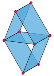
Figure 2: The Vamos matroid of size $8$ and rank $4$, which is not algebraically representable.

A third example of matroids occurring naturally in mathematics are algebraic matroids algebraic . These are associated to field extensions $\mathbb{F}:K$ together with a finite point sets $E\subseteq K$, where the independent sets are those $I\subseteq E$ that are algebraically independent over $\mathbb{F}$. In particular, elements that are algebraic over $\mathbb{F}$ have rank zero, and in general $\rho(I)$ is the transcendence degree of the field extension $\mathbb{F}(I):\mathbb{F}$.

It is rather easy to see that every $\mathbb{F}$-linear matroid is also algebraic over $\mathbb{F}$. Indeed, let $X_{1},\cdots,X_{k}$ be indeterminates, and let

$$g:\mathbb{F}^{k}\to\mathbb{F}(X_{1},\cdots,X_{k})$$

be given by $\mathrm{e}_{i}\mapsto X_{i}$ for $i=1,\cdots k$. Then $J\subseteq E$ is linearly independent over $\mathbb{F}$ if and only if $\{g(j):j\in J\}$ is algebraically independent over $\mathbb{F}$. Over fields of characteristic zero the converse also holds, so that all algebraic matroids have a linear representation. However, in positive characteristic there exist algebraic matroids that are not linearly representable. For example, the non-Pappus matroid of Example 4 is algebraically representable over $\mathbb{F}_{4}$, although it is not linearly representable over any field lindstrom88 . The smallest example of a matroid that is not algebraic over any field is the Vamos matroid, in Figure 2 ingleton75 .

Definition 21

The dual of $M=(\rho,E)$ is $M^{*}=(\rho^{*},E)$, where

$$\rho^{*}(X)=|X|+\rho(E\setminus X)-\rho(E).$$

The definition of the dual matroid lies in the heart of matroid theory, and has profound interpretations. In geometric terms, let $M$ be represented by a $k$-dimensional subspace $V$ of $\mathbb{F}^{n}$. Then, the matroid dual $M^{*}$ is represented by the orthogonal complement $V^{\perp}\subseteq\mathbb{F}^{n}$. Surprisingly and seemingly unrelatedly, if $\Gamma$ is a planar graph and $M=M_{\Gamma}$ is a graphical matroid, then $M^{*}=M_{\bar{\Gamma}}$, where $\bar{\Gamma}$ is the planar dual of $\Gamma$. Moreover, the dual $M_{\Gamma}^{*}$ of a graphical matroid is graphical if and only if $\Gamma$ is planar.

Definition 22

The contraction of $X\subseteq E$ in the matroid $M=(\rho,E)$ is $M/X=(\rho^{\prime},M\setminus X)$, where $\rho^{\prime}(Y)=\rho(Y\cup X)-\rho(X)$.

Contraction is the dual operation of deletion, in the sense that $M/X=(M^{*}_{|E\setminus X})^{*}$. The terminology comes from graphical matroids, where contraction of the edge $e\in E$ corresponds to deleting $e$ and identifying its endpoints in the graph. Notice that it follows directly from submodularity of the rank function that $\rho_{M/X}(Y)\leq\rho_{M|_{E\setminus X}}(Y)$ for every $Y\subseteq E\setminus X$. In terms of subspace representations, contraction of $e\in E$ corresponds to intersecting the subspace that represents $M$ with the hyperplane $\{x_{e}=0\}$.

As matroids are used as an abstraction for linear codes, it would be desirable to have a way to go back from matroids to codes, namely to determine whether a given matroid is representable, and when it is, to find such a representation. Unfortunately, there is no simple criterion to determine representability vamos78 ; mayhew14 . However, there are a plethora of sufficient criteria to prove nonrepresentability, both over a given field and over fields in general. In recent years, these methods have been used to prove two long-standing conjectures, that we will discuss in Sections 6.1 and 6.2 respectively.

6.1 Rota’s Conjecture

While there is no simple criterion to determine linear representability, the situation is much more promising if we consider representations over a fixed field. It has been known since 1958, that there is a simple criterion for when a matroid is binary representable.

Theorem 6.1 (tutte58 )

Let $M=(\rho,E)$ be a matroid. The following two conditions are equivalent.

1. $M$ is linearly representable over $\mathbb{F}_{2}$.

2. There are no sets $X\subseteq Y\subseteq E$ such that $M|Y/X$ is isomorphic to the uniform matroid $U_{4}^{2}$.

In essence, this means that the only obstruction that needs to be overcome in order to be representable over the binary alphabet, is that no more than three nonzero points can fit in the same plane. For further reference, we say that a minor of the matroid $M=(\rho,E)$ is a matroid of the form $M|Y/X$, for $X\subseteq Y\subseteq E$. Clearly, if $M$ is representable over $\mathbb{F}$, then so is all its minors. Let $L(\mathbb{F})$ be the class of matroids that are not representable over $\mathbb{F}$, but such that all of their minors are $\mathbb{F}$-representable. Then the class of $\mathbb{F}$-representable matroids can be written as the class of matroids that does not contain any matroid from $L(\mathbb{F})$ as a minor. Gian-Carlo Rota conjectured in 1970 that $L(\mathbb{F})$ is a finite set for all finite fields $\mathbb{F}$. A proof of this conjecture was announced by Geelen, Gerards and Whittle in 2014, but the details of the proof still remain to written up whittle14 .

Theorem 6.2

For any finite field $\mathbb{F}$, there is a finite set $L(\mathbb{F})$ of matroids such that any matroid $M$ is representable if and only if it contains no element from $L(\mathbb{F})$ as a minor.

Since the 1970’s, it has been known that a matroid is representable over $\mathbb{F}_{3}$ if and only if it avoids the uniform matroids $U_{5}^{2}$, $U_{5}^{3}$, the Fano plane $P^{2}(\mathbb{F}_{2})$, and its dual $P^{2}(\mathbb{F}_{2})^{*}$ as minors. The list $L(\mathbb{F}_{4})$ has seven elements, and was given explicitly in 2000. For larger fields, the explicit list is not known, and there is little hope to even find useful bounds on its size.

6.2 Most Matroids are Nonrepresentable

For a fixed finite field $\mathbb{F}$, it follows rather immediately from the minor-avoiding description in the last section that the fraction of $n$-symbol matroids that is $\mathbb{F}$-representable goes to zero as $n\to\infty$. It has long been a folklore conjecture that this is true even when representations over arbitrary fields are allowed. However, it was only in 2016 that a verifiable proof of this claim was announced nelson16 .

Theorem 6.3

$$\lim_{n\rightarrow\infty}\frac{\#\hbox{linear matroids on $n$ elements}}{\#\hbox{matroids on $n$ elements}}=0.$$

The proof is via estimates of the denominator and enumerator of the expression in 6.3 separately. Indeed, it is shown in knuth74 that the number of matroids on $n$ nodes is at least $\Omega(2^{(2-\varepsilon)^{n}})$ for every $\epsilon>0$. The proof of Theorem 6.3 thus boiled down to proving that the number of representable matroids is $O(2^{n^{3}})$. This is in turn achieved by bounding the number of so called zero-patterns of polynomials.

6.3 Gammoid Construction of Singleton-Optimal LRCs

For completeness, we end this appendix with a theorem that explicitly presents the matroids constructed in Theorem 4.1 as gammoids. As discussed in Section4.2, this proves the existence of Singleton-optimal linear LRCs whenever a set system satisfying (8) exists.

Theorem 6.4 (westerback15 , $M(F_{1},\ldots,F_{m},E;k;\rho)$-matroids are gammoids)

Let $M(F_{1},\ldots,F_{m};\rho)$ be a matroid given by Theorem 4.1 and define $s:E\rightarrow 2^{[m]}$ where $s(x)=\{i\in[m]:x\in F_{i}\}$. Then $M(F_{1},\ldots,F_{m},E;k;\rho)$ is equal to the gammoid $M(\Gamma,E,T)$, where $\Gamma=(V,D)$ is the directed graph with

$$\begin{array}[]{rl}(i)&V=E\cup H\cup T\hbox{ where }E,H,T\hbox{ are pairwise disjoint},\\ (ii)&T=[k],\\ (iii)&H\hbox{ equals the union of the pairwise disjoint sets}\\ &\hbox{$H_{1},\ldots,H_{m},H_{\geq 2}$, where}\\ &\begin{array}[]{l}|H_{i}|=\rho(F_{i})-|\{x\in F_{i}:|s(x)|\geq 2\}|\hbox{ for }i\in[m],\\ H_{\geq 2}=\{h_{y}:y\in E\hbox{, }|s(y)|\geq 2\},\\ \end{array}\\ (iv)&D=D_{1}\cup D_{2}\cup D_{3}\hbox{, where}\\ &\begin{array}[]{l}D_{1}=\bigcup_{i\in[m]}\{(\overrightarrow{x,y}):x\in E\hbox{, }s(x)=\{i\}\hbox{, }y\in H_{i}\},\\ D_{2}=\{(\overrightarrow{x,h_{y}}):x\in E\hbox{, }h_{y}\in H_{\geq 2}\hbox{, }s(x)\subseteq s(y)\},\\ D_{3}=\{(\overrightarrow{x,y}):x\in H,y\in T\}.\\ \end{array}\end{array}$$

References

- (1) Ball, S.: On sets of vectors of a finite vector space in which every subset of basis size is a basis. Journal of the European Mathematical Society 14, 733–748 (2012)
- (2) Barg, A., Haymaker, K., Howe, E., Matthews, G., Várilly-Alvarado, A.: Locally recoverable codes from algebraic curves and surfaces (2017). ArXiv: 1701.05212
- (3) Barg, A., Tamo, I., Vlăduţ, S.: Locally recoverable codes on algebraic curves (2016). ArXiv: 1603.08876
- (4) Bonin, J.E., de Mier, A.: The lattice of cyclic flats of a matroid. Annals of combinatorics 12, 155–170 (2008)
- (5) Britz, T., Rutherford, C.G.: Covering radii are not matroid invariants. Discrete Mathematics 296, 117–120 (2005)
- (6) Cadambe, V., Mazumdar, A.: An upper bound on the size of locally recoverable codes. In: International Symposium on Network Coding, pp. 1–5 (2013)
- (7) Dimakis, A., Godfrey, P.B., Wu, Y., Wainwright, M.J., Ramchandran, K.: Network coding for distributed storage systems. IEEE Transactions on Information Theory 56(9), 4539–4551 (2010)
- (8) Ernvall, T., Westerbäck, T., Freij-Hollanti, R., Hollanti, C.: Constructions and properties of linear locally repairable codes. IEEE Transactions on Information Theory 62, 5296–5315 (2016)
- (9) Fazeli, A., Vardy, A., Yaakobi, E.: Pir with low storage overhead: coding instead of replication. arXiv:1505.06241 (2015)
- (10) Freij-Hollanti, R., Westerbäck, T., Hollanti, C.: Locally repairable codes with availability and hierarchy: matroid theory via examples. In: International Zürich Seminar on Communications, pp. 45–49. IEEE/ETH (2016)
- (11) Fujishige, S.: Polymatroidal dependence structure of a set of random variables. Information and control 39(1), 55–72 (1978)
- (12) Geelen, J., Gerards, B., Whittle, G.: Solving Rota’s conjecture. Notices of the American Mathematical Society 61(736–743) (2014)
- (13) Gopalan, P., Huang, C., Simitci, H., Yekhanin, S.: On the locality of codeword symbols. IEEE Transactions on Information Theory 58(11), 6925–6934 (2012)
- (14) Huang, C., Chen, M., Lin, J.: Pyramid codes: Flexible schemes to trade space for access efficiency in reliable data storage systems. In: International Symposium on Network Computation and Applications, pp. 79–86. IEEE (2007)
- (15) Ingleton, A., Main, R.: Non-algebraic matroids exist. Bulletin of the London Mathematical Society 7(144–146) (1975)
- (16) Ishai, Y., Kushilevitz, E., Ostrovsky, R., Sahai, A.: Batch codes and their applications. In: The 36th ACM Symposium on Theory of Computing (STOC) (2004)
- (17) Jurrius, R., Pellikaan, R.: Truncation formulas for invariant polynomials of matroids and geometric lattices. Mathematics in Computer Scinece 6, 121–133 (2012)
- (18) Kamath, G.M., Prakash, N., Lalitha, V., Kumar, P.V.: Codes with local regeneration and erasure correction. IEEE Transactions on Information Theory 60(8), 4637–4660 (2014)
- (19) Knuth, D.: The asymmetric number of geometries. Journal of Combinatorial Theory, Series A 16, 398–400 (1974)
- (20) Lindström, B.: On the vector representations of induced matroids. Bulletin of the London Mathematical Society 5, 85–90 (1973)
- (21) Lindström, B.: On -polynomial representations of projective geometries in algebraic combinatorial geometries. Mathematica Scandinavica 63, 36–42 (1988)
- (22) Lindström, B.: On algebraic matroids. Discrete Mathematics 111(357–359) (1993)
- (23) Lipmaa, H., Skachek, V.: Linear batch codes. In: The 4th International Castle Meeting on Coding Theory and Applications (4ICMCTA) (2015)
- (24) Mayhew, D., Newman, M., Welsh, D., Whittle, G.: On the asymptotic proportion of connected matroids. European Journal of Combinatorics 32(6), 882–890 (2011)
- (25) Mayhew, D., Newman, M., Whittle, G.: Yes, the missing axiom of matroid theory is lost forever (2015). ArXiv: 1412.8399
- (26) Nelson, P.: Almost all matroids are non-representable. ArXiv: 1605.04288
- (27) Papailiopoulos, D., Dimakis, A.: Locally repairable codes. In: International Symposium on Information Theory, pp. 2771–2775. IEEE (2012)
- (28) Pendavingh, R., van der Pol, J.: On the number of matroids compared to the number of sparse paving matroids. Electronic Journal of Combinatorics 22, 17pp. (2015)
- (29) Pöllänen, A., Westerbäck, T., Freij-Hollanti, R., Hollanti, C.: Improved singleton-type bounds for locally repairable codes. In: International Symposium on Information Theory, pp. 1586–1590. IEEE (2016)
- (30) Prakash, N., Kamath, G.M., Lalitha, V., Kumar, P.V.: Optimal linear codes with a local-error-correction property. In: International Symposium on Information Theory, pp. 2776–2780. IEEE (2012)
- (31) Rawat, A.S., Papailiopoulos, D., Dimakis, A., Vishwanath, S.: Locality and availability in distributed storage (2014). ArXiv: 1402.2011v1
- (32) Sasidharan, B., Agarwal, G.K., Kumar, P.V.: Codes with hierarchical locality (2015). ArXiv: 1501.06683v1
- (33) Silberstein, N., Rawat, A.S., Koyluoglu, O., Vishwanath, S.: Optimal locally repairable codes via rank-metric codes. In: International Symposium on Information Theory, pp. 1819–1823. IEEE (2013)
- (34) Silberstein, N., Zeh, A.: Optimal binary locally repairable codes via anticodes (2015). ArXiv: 1501.07114v1
- (35) Sims, J.A.: Some problems in matroid theory. Ph.D. thesis, Oxford University (1980)
- (36) Singleton, R.C.: Maximum distance q-nary codes. IEEE Transactions on Information Theory 10(2), 116–118 (1964)
- (37) Skorobogatov, A.: Linear codes, strata of grassmannians, and the problems of segre. In: International Workshop on Coding Theory and Algebraic Geometry, pp. 210–223 (1992)
- (38) Song, W., amd C. Yuen, S.H.D., Li, T.J.: Optimal locally repairable linear codes. IEEE Journal on Selected Areas in Communications 32(5), 1019–1036 (2014)
- (39) Tamo, I., Barg, A.: A family of optimal locally recoverable codes. IEEE Transactions on Information Theory 60(8), 4661–4676 (2014)
- (40) Tamo, I., Barg, A., Frolov, A.: Bounds on the parameters of locally recoverable codes. IEEE Transactions on Information Theory 62(6), 3070–3083 (2016)
- (41) Tamo, I., Papailiopoulos, D., Dimakis, A.: Optimal locally repairable codes and connections to matroid theory. In: International Symposium on Information Theory, pp. 1814–1818. IEEE (2013)
- (42) Tutte, W.: A homotopy theorem for matroids, I, II. Transactions of the Amarican Mathematical Society 88, 148–178 (1958)
- (43) Vámos, P.: The missing axiom of matroid theory is lost forever. Journal of the London Mathematical Society 18, 403–408 (1978)
- (44) Wang, A., Zhang, Z.: Repair locality with multiple erasure tolerance. IEEE Transactions on Information Theory 60(11), 6979–6987 (2014)
- (45) Wang, A., Zhang, Z.: An integer programming-based bound for locally repairable codes. IEEE Transactions on Information Theory 61(10), 5280–5294 (2015)
- (46) Westerbäck, T., Freij, R., Hollanti, C.: Applications of polymatroid theory to distributed storage systems. In: Allerton Conference on Communication, Control, and Computing, pp. 231–237 (2015)
- (47) Westerbäck, T., Freij-Hollanti, R., Ernvall, T., Hollanti, C.: On the combinatorics of locally repairable codes via matroid theory. IEEE Transactions on Information Theory 62, 5296–5315 (2016)
- (48) Whitney, H.: On the abstract properties of linear dependence. American Journal of Mathematics 57, 509–533 (1935)
- (49) Zhang, H., Skachek, V.: Bounds for batch codes with restricted query size. In: IEEE International Symposium on Information Theory (ISIT) (2016)