journalname
A Tutorial on Kernel Density Estimation and Recent Advances
Yen-Chi Chen
Department of Statistics
University of Washington
This tutorial provides a gentle introduction to kernel density estimation (KDE) and recent advances regarding confidence bands and geometric/topological features. We begin with a discussion of basic properties of KDE: the convergence rate under various metrics, density derivative estimation, and bandwidth selection. Then, we introduce common approaches to the construction of confidence intervals/bands, and we discuss how to handle bias. Next, we talk about recent advances in the inference of geometric and topological features of a density function using KDE. Finally, we illustrate how one can use KDE to estimate a cumulative distribution function and a receiver operating characteristic curve. We provide R implementations related to this tutorial at the end.
Keywords: kernel density estimation, nonparametric statistics, confidence bands, bootstrap
1 Introduction
Kernel density estimation (KDE), also known as the Parzen’s window (Parzen, 1962), is one of the most well-known approaches to estimate the underlying probability density function of a dataset. KDE is a nonparametric density estimator requiring no assumption that the underlying density function is from a parametric family. KDE will learn the shape of the density from the data automatically. This flexibility arising from its nonparametric nature makes KDE a very popular approach for data drawn from a complicated distribution.
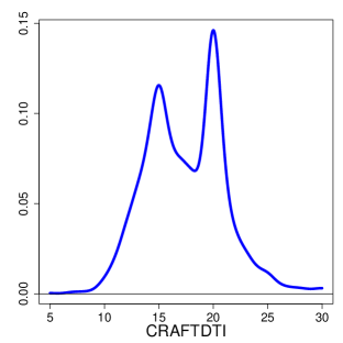
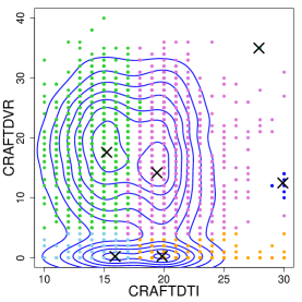
Figure 1 illustrates KDE using a part of the NACC (National Alzheimer s Coordinating Center) Uniform Data Set (Beekly et al., 2007), version 3.0 (March 2015). Because the purpose of using this dataset is to illustrate the effectiveness of KDE, we will draw no scientific conclusion but will just use KDE as a tool to explore the pattern of the data. We focus on two variables, ‘CRAFTDTI’ (Craft Story 21 Recall – delay time), and ‘CRAFTDVR’ (Craft Story 21 Recall – total story units recalled, verbatim scoring). Although these two variables take integer values, we treat them as continuous and use KDE to determine the density function. We consider only the unique subject with scores on both variables, resulting in a sample of size . In the left panel of Figure 1, we display the estimated density function of ‘CRAFTDTI’ using KDE. We see that there are two modes in the distribution. In the right panel of Figure 1, we show the scatter plot of the data and overlay it with the result of bivariate KDE (blue contours). Because many subjects have identical values for the two variables, the scatter plot (gray dots) provides no useful information regarding the underlying distribution. However, KDE shows the multi-modality of this bivariate distribution, which contains multiple bumps that cannot be captured easily by any parametric distribution.
The remainder of the tutorial is organized as follows. In Section 2, we present the definition of KDE, followed by a discussion of its basic properties: convergence rates, density derivative estimations, and bandwidth selection. Then, in Section 3, we introduce common approaches to the construction of confidence regions, and we discuss the problem of bias in statistical inference. Section 4 provides an introduction to the use of KDE to estimate geometric and topological features of a density function. In Section 5, we study how one can use KDE to estimate the cumulative distribution function (CDF) and the receiver operating characteristic (ROC) curve. Finally, in Section 6, we discuss open problems. At the end of this tutorial, we provide R codes for implementing the presented analysis of KDE.

2 Statistical Properties
Let be an independent, identically distributed random sample from an unknown distribution with density function . Formally, KDE can be expressed as
| (1) |
where is a smooth function called the kernel function and is the smoothing bandwidth that controls the amount of smoothing. Two common examples of are
Note that we apply the same amount of smoothing in every direction; in practice, one can use a bandwidth matrix and the quantity becomes .
Intuitively, KDE has the effect of smoothing out each data point into a smooth bump, whose the shape is determined by the kernel function . Then, KDE sums over all these bumps to obtain a density estimator. At regions with many observations, because there will be many bumps around, KDE will yield a large value. On the other hand, for regions with only a few observations, the density value from summing over the bumps is low, because only have a few bumps contribute to the density estimate.
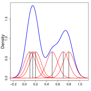
Figure 2 presents examples of KDE in the 1D case. There are six observations, as indicated by the black lines. We smooth these observations into bumps (red bumps) and sum over all of the bumps to form the final density estimator (the blue curve). In R, many packages are equipped with programs for computing KDE; see Deng and Wickham (2011) for a listing.
Remark. (Adaptive smoothing) The amount of smoothing can depend on the location (Loftsgaarden and Quesenberry, 1965) or the data point (Breiman et al., 1977). In the former case, we use so KDE becomes which is referred to as the balloon estimator (Terrell and Scott, 1992). In the latter case, we use for the -th data points with the resulting density estimate being which is referred to as the sample smoothing estimator (Terrell and Scott, 1992). For more details regarding adaptive smoothing, we refer the readers to Section 6.6 of Scott (2015).
2.1 Convergence Rate
To measure the errors of KDE, we consider three types of errors: the pointwise error, uniform error, and mean integrated square error (MISE). The pointwise error is the simplest error and is related to the confidence interval (Section 3.1). The uniform error has many useful theoretical properties since it measures the uniform deviation of the estimator and can be used to bound other types of errors. The uniform error is related to the confidence band and the geometric (and topological) features; see Section 3.2 and Section 4. The MISE (actually it is a risk measurement of the estimator) is generally used in bandwidth selection (Section 2.3), because it measures the overall performance of the estimator and is related to the mean square error.
Pointwise Error. For a given point , the pointwise error of KDE is the difference between KDE and , the true density function evaluated at . Let be the Laplacian of the function . Under smoothness conditions (Scott, 2015; Wasserman, 2006; Tsybakov, 2009),
| (2) | ||||
where and are constants depending only on the kernel function . Thus, when and , , i.e., KDE is a consistent estimator of . Equation (2) presents the decomposition of the (pointwise) estimation error of KDE in terms of the bias and the stochastic variation . This decomposition will be used frequently in deriving other errors and constructing the confidence regions.
Uniform Error. Another error metric is the uniform error (also known as the error), the maximal difference between and : . According to empirical process theory (Yukich, 1985; Giné and Guillou, 2002; Einmahl and Mason, 2005; Rao, 2014), the uniform error
| (3) |
under mild conditions (see Giné and Guillou (2002); Einmahl and Mason (2005) for more details). The error rate in (3) and the pointwise error rate in (2) differ only in the stochastic variation portion and the difference is at the rate . The presence of an extra in the uniform error rate is a very common phenomenon in nonparametric estimation owing to empirical process theory. The uniform error has many useful theoretical properties (Chen et al., 2015c; Chen, 2016; Fasy et al., 2014; Jisu et al., 2016), because it provides a uniform control of the estimation error over the entire support.
MISE. The MISE is one of the most well-known error measurements (Wasserman, 2006; Scott, 2015) among all of the error measures used in KDE. The MISE is defined as . Thus, the MISE measures the risk of KDE. Under regularity conditions, the MISE
| (4) | ||||
The MISE can be viewed as the mean square error of KDE. The dominating term is called the asymptotic mean integrated square error (AMISE). Equation (4) shows that the error (risk) of KDE can be decomposed in to a bias component, , and a variance component together with small corrections. This decomposition is known as the bias-variance tradeoff (Wasserman, 2006) and is very useful in practice because we can choose the smoothing bandwidth by optimizing this error. If we ignore smaller order terms and use the AMISE, the minimal error occurs when we choose
| (5) |
which leads to the optimal MISE
Equation (5) will be a key result in choosing the smoothing bandwidth (Section 2.3). Note that in practice, people generally select the smoothing bandwidth by minimizing the MISE rather than other errors because (i) it is a risk function that does not depend on any particular sample, (ii) it measures the overall estimation error rather than putting too much weight on a small portion of the support (i.e., it is more robust to small perturbations), and (iii) it has useful theoretical behaviors, including the expression of the bias-variance tradeoff and the connection to the mean square error.
Remark. (Boundary bias) When the density function is discontinuous, the bias of KDE at the discontinuities will be of the order rather than , and this bias is called the boundary bias (Wasserman, 2006; Scott, 2015). In practice, one can use the boundary kernel to reduce the boundary bias (see, e.g., Chapter 6.2.3.5 in Scott (2015)).
2.2 Derivative Estimation
KDE can be used to estimate the derivative of the density function. This is often called density derivative estimation (Stoker, 1993; Chacón et al., 2011). The idea is simple: we use the derivative of KDE as an estimator of the corresponding derivative of the density function. Let be a multi-index (each is a non-negative integer and ). Define to be the -th order partial derivative operator. For instance, implies and . Then, under smoothness assumptions (Chacón et al., 2011),
| (6) |
That is, the (MISE or pointwise) error rate of gradients of KDE is and the error rate of second derivatives (Hessian matrix) of KDE is . Similarly to and in the density estimation, there are explicit formulas for the bias and stochastic variation of density derivative estimation; see Chacón et al. (2011) for more details. Some examples of using gradient and second derivative estimation can be found in Arias-Castro et al. (2016); Chacón and Duong (2013); Chen et al. (2015b, c); Genovese et al. (2009, 2014).
2.3 Bandwidth Selection
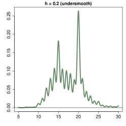
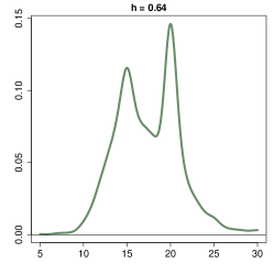
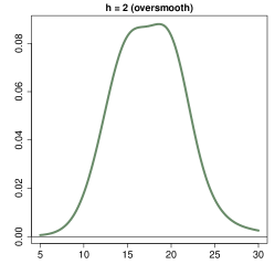
How to choose the smoothing bandwidth for KDE is a classical research topic in nonparametric statistics. This problem is often known as bandwidth selection. Figure 3 shows KDE’s with different amounts of smoothing of the same dataset. When is too small (left panel), there are many wiggles in the density estimate. When is too large (right panel), we smooth out important features. When is at the correct amount (middle), we can see a clear picture of the underlying density.
Common approaches to bandwidth selection include the rule of thumb (Silverman, 1986), least square cross-validation, (Rudemo, 1982; Bowman, 1984; Bowman and Azzalini, 1997; Stone, 1984), biased cross-validation, (Scott and Terrell, 1987), and plug-in method (Woodroofe, 1970; Sheather and Jones, 1991). Roughly speaking, the core idea behind all of these methods is to minimize the AMISE, the dominating quantity in the MISE (4), or other similar error measurements. Different bandwidth selectors can be viewed as different estimators to the AMISE, and is chosen by minimizing the AMISE estimator. Overviews and comparisons of the existing methods can be found in Jones et al. (1996); Sheather (2004), page 135–137 in Wasserman (2006), and Chapter 6.5 in Scott (2015).
While most of the literature focuses on the univariate case, Chacón and Duong (2013) provides a generalization of all of the above methods to the multivariate case and also generalizes the AMISE criterion into density derivative estimation. In R, one can use packge ‘ks111https://cran.r-project.org/web/packages/ks/index.html’ or ‘kedd222https://cran.r-project.org/web/packages/kedd/index.html’ to choose smoothing bandwidths for both density estimation and density derivative estimation. Note that the ks package is applicable to multivariate data.
In addition to the above approaches, Goldenshluger and Lepski (2011) propose a method, known as the Lepski’s approach (Goldenshluger and Lepski, 2008; Lepski and Goldenshluger, 2009), that treats the bandwidth selection problem as a model selection problem and proposes a new criterion for selecting the smoothing bandwidth. One feature of Lepski’s approach is that the selected bandwidth enjoys many statistical optimalities (Goldenshluger and Lepski, 2011).
Remark. (Kernel Selection) In contrast to bandwidth selection, the choice of kernel function does not play an important role in KDE. The effect of the kernel function on the estimation error is just a constant shift (via and in equation (2)), and the difference is generally very small among common kernel functions (see, e.g., page 72 of Wasserman (2006) and Section 6.2.3 in Scott (2015)), so most of the literature ignore this topic.
3 Confidence Intervals and Confidence Bands
Confidence regions of the density function are random intervals derived from the sample such that covers the true value of with probability at least . Based on this notion, there are two common types of confidence regions:
-
•
Confidence interval: for a given , the set satisfies
-
•
Confidence band: the interval satisfies
Namely, confidence intervals are confidence regions with only local coverage and confidence bands are confidence regions with simultaneous coverage. If a confidence interval/band has only coverage , it will be called an asymptotically valid confidence interval/band.
For simplicity, we first ignore the bias between and by assuming in Sections 3.1 and 3.2 (i.e., we assume ). We will discuss strategies for handling the bias in Section 3.3
3.1 Confidence Intervals
For a given point , by equation (2),
| (7) |
where . Equation (7) implies that a straight-forward approach to construct a confidence band is to use asymptotic normality with a variance estimator.
Method 1: Plug-in Approach. A simple method is replacing in the asymptotic variance by its estimator , leading to the following confidence interval of :
| (8) |
We call this method the “plug-in method” because we plug-in the variance estimator to construct a confidence interval. When , is a consistent estimator of . As a result,
Method 2: Bootstrap and Plug-in Approach. An alternative method is to estimate the asymptotic variance using the bootstrap (Efron, 1979). In more detail, we use the empirical bootstrap (also known as the nonparametric bootstrap or Efron’s bootstrap, which is to sample the original data with replacement) to generate bootstrap sample . Then, we apply KDE to the bootstrap sample, resulting in a bootstrap KDE . When we repeat the bootstrap times, we then have bootstrap KDEs . Let
where is the sample average of the bootstrap KDE’s. Namely, is the sample variance of the bootstrap KDE’s evaluated at . A bootstrap confidence interval is
| (9) |
Because the bootstrap variance estimator converges to in the sense that
the bootstrap variance estimator is consistent, so the confidence interval will also be consistent:
Method 3: Bootstrap Approach. In addition to the above methods, one can use a fully bootstrapping approach to construct a confidence interval without using asymptotic normality. Let be bootstrap KDE’s as in the previous method. We define a pointwise deviation of a bootstrap KDE by
Then we compute the quantile of the empirical CDF of :
A confidence interval of is
| (10) |
Because the distribution of approximates the distribution of , this confidence interval is also asymptotically valid, i.e.,
3.1.1 Example: Confidence Intervals
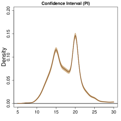
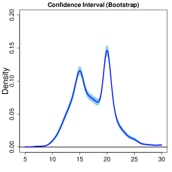
In Figure 4, we compare the three approaches of constructing a confidence interval using the NACC Uniform Data Set, as described in the Introduction (Section 1) and the left panel of Figure 1. The left panel is the 95% confidence interval of each point using the plug-in approach (method 1); the middle panel is the 95% confidence interval from the plug-in and bootstrap approach (method 2); the right panel is the 95% confidence interval from the bootstrap approach (method 3).
Essentially, the three confidence intervals are very similar; in particular, the confidence intervals from the method 2 and 3 are nearly identical. The interval from method 1 is slightly smaller than the other two.
While all of these intervals are valid for each given point, there is no guarantee that they will cover the entire density function simultaneously. In the next section, we introduce methods of constructing confidence bands (confidence regions with simultaneous coverage).
3.2 Confidence Bands
Now, we present methods of constructing confidence bands. The key idea is to approximate the distribution of the uniform error and then convert it into a confidence band. To be more specific, let be the CDF of the uniform error, and let be the quantile. Then it can be shown that the set
is a confidence band, i.e.,
Therefore, as long as we have a good approximation of the distribution , we can convert the approximation into a confidence band.
Method 1: Plug-in Approach. An intuitive approach is to derive the asymptotic distribution of directly and then invert it into a confidence band. Bickel and Rosenblatt (1973); Rosenblatt et al. (1976) proved that the uniform loss converges to an extreme value distribution in the sense that
| (11) |
where is a quantity depending only on and the kernel function . Rosenblatt et al. (1976) provided an exact expression for the quantity . Let be the quantile of the right-hand-side CDF. Define
Then, by equation (11), falls within with probability at least (asymptotically) . To construct a confidence band, we replace the quantity in with a plug-in estimate from KDE, leading to
Then a confidence band will be
| (12) |
Although equation (12) is an asymptotically valid confidence band, the convergence to the extreme value distribution in equation (11) is very slow Hall (1991). Thus, we need a huge sample size to guarantee that the confidence band from (12) is asymptotically valid. To resolve this problem, we use the bootstrap.
Method 2: Bootstrap Approach. The key element of how the bootstrap works is that the uniform error can be approximated accurately by the supremum of a Gaussian process (Neumann, 1998; Chernozhukov et al., 2014b, c). In more detail, there exists a tight Gaussian process such that
| (13) |
Moreover, the difference between the bootstrap KDE and the original KDE also has a similar convergent result (Chernozhukov et al., 2013, 2014a, 2016):
| (14) |
where is the same Gaussian process as the one in equation (13). Thus, the distribution of will be approximated by the distribution of its bootstrap version . As a result, the bootstrap quantile of uniform error converges to the quantile of the actual uniform error, thereby proving that the bootstrap confidence band is asymptotically valid.
Here is the formal construction of a bootstrap confidence band. Let be the bootstrap KDE’s. We define the uniform deviation of the bootstrap KDE’s by
Then, we compute the quantile of the empirical CDF of as
A confidence band will be
| (15) |
By equations (13) and (14), when ,
Namely, the set is an asymptotically valid confidence band.
3.2.1 Example: Confidence Bands
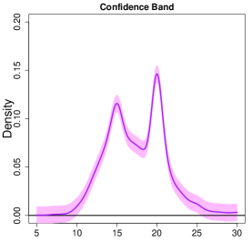
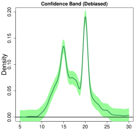
Figure 5 presents confidence bands using KDE. The left panel shows the confidence band from the bootstrap approach introduced in the previous section. Compared to the confidence intervals in Figure 4, the confidence bands are wider because we need to control the coverage simultaneously for every point.
However, the confidence band in the left panel of Figure 5 (and all of the confidence intervals in Figure 4) has a serious problem–the coverage guarantee is for the expected value of KDE rather than for the true density function . Unless we undersmooth KDE (choose converging at a faster rate than ), the confidence band shows undercoverage. We will discuss this topic in more detail in Section 3.3.
To construct an (asymptotically valid) confidence band with being at rate , we use the debiased estimator introduced in Chen (2017). The details are provided in Section 3.3.3 and Figure 6. The right panel of Figure 5 shows a confidence band from the debiased KDE approach. Although the confidence band is wider, the coverage is guaranteed for such a confidence band.
3.3 Handling the Bias
In the previous section, we ignored the bias in KDE. However, the bias could be a severe problem in reality because it systematically shifted our confidence interval/band so the actual coverage is below the nominal coverage. Here we discuss strategies to handle bias.
3.3.1 Ignoring the Bias
A simple strategy is to ignore the bias and focus on inferring the expectation of KDE . is called the smoothed or mollified density function (Rinaldo and Wasserman, 2010; Chen et al., 2015b, c). As long as the kernel function is smooth, will also be smooth. Moreover, exists even when the distribution function is singular (in this case, the population density does not exist). For inferring geometric or topological features, might be a better parameter of interest because structures in generally represent salient structures of (Chen et al., 2015c) and many topological structures of will be similar to those of when is small (Chen et al., 2015b; Genovese et al., 2014; Jisu et al., 2016). If we switch our target to , we have to make it clear that this is a confidence region of rather than of when we report our confidence regions.
3.3.2 Undersmoothing
Undersmoothing is a very common approach to handle bias in KDE (and other nonparametric approaches). Recall from equation (2):
The bias is , and the stochastic variation is the term. If now we take such that , then the stochastic variability dominates the errors. Therefore, we can ignore the bias term and use the method suggested in Section 3.1 and 3.2.
Note that is equivalent to , which corresponds to choosing a smaller smoothing bandwidth than the optimal smoothing bandwidth () that balances the bias and the variance (this is why it is called undersmoothing). Although the undersmoothing provides a valid construction of confidence regions, such a choice of bandwidth implies that the size of the confidence band is larger than the optimal size because we are inflating the variance to eliminate the bias. Some references to undersmoothing can be found in Bjerve et al. (1985); Hall (1992a); Hall and Owen (1993); Chen (1996); Neumann and Polzehl (1998); Chen and Qin (2002); McMurry and Politis (2008).
3.3.3 Bias-corrected and Oversmoothing
An alternative approach to construct a valid confidence band is to correct the bias of KDE explicitly; this approach is known as the bias-corrected method and the resulting KDE is called the bias-corrected KDE. Recall from equation (2) that the bias in KDE is
Thus, we can correct the bias by estimating . The quantity can be estimated by , where
is KDE using smoothing bandwidth . Recall from Section 2.2 that the second derivative estimator has an error rate
| (16) |
Thus, to obtain a consistent estimator of , we have to choose another smoothing bandwidth , and this smoothing bandwidth needs to be larger than the optimal bandwidth . Because the choice of corresponds to oversmoothing KDE, this approach is also called the “oversmoothing” method.
Using , the bias-corrected KDE is
When is a consistent estimator of , the pointwise error rate is
so the dominating quantity, , is the stochastic variation in . Thus, the confidence regions can be constructed by replacing by in equations (8), (9), (10), and (15). An incomplete list of literature of the bias-corrected approach is as follows: Härdle and Bowman (1988); Hardle and Marron (1991); Hall (1992b); Eubank and Speckman (1993); Sun and Loader (1994); Härdle et al. (1995); Neumann (1995); Xia (1998); Härdle et al. (2004).
Calonico et al. (2015) proposes a plug-in method of constructing a confidence interval with . Although the choice does not lead to a consistent estimate of the second derivative, the bias will be pushed into the next order because the bias-corrected estimator can be viewed as a higher order kernel function (see page 157 in Scott (2015)). Thus, since the dominating term in the estimation error is the stochastic variation, we can construct an asymptotically valid confidence interval using the plug-in approach.
Chen (2017) further generalizes the idea of Calonico et al. (2015) to confidence bands by bootstrapping the bias-corrected kernel density estimator with . Figure 6 summarizes the procedure of constructing a confidence band using the approach in Chen (2017). The resulting confidence band, , has the following property:
when . Namely, is an asymptotically valid confidence band when we pick under the optimal rate. The right panel of Figure 5 shows an example of this confidence band. Although this approach generally leads to a wider confidence band, this confidence band has asymptotically coverage whereas the confidence band in the left panel of Figure 5 has undercoverage.
Confidence Band of Density Function. 1. Choose the smoothing bandwidth by a standard approach such as the rule of thumb or cross-validation (Silverman, 1986; Sheather and Jones, 1991; Sheather, 2004). 2. Compute the bias-corrected KDE (with in equation (16)) 3. Bootstrap the original sample for times and compute the bootstrap bias-corrected KDE 4. Compute the quantile 5. Output the confidence band
Remark. (Calibration) In addition to the above methods, another possible approach is to choose a corrected coverage of confidence regions; this approach is called “calibration” and is related to the work in Beran (1987); Hall (1986); Loh (1987); Hall and Horowitz (2013). The principal idea is to investigate the effect of the bias on the coverage of the confidence band and then choose a conservation quantile to guarantee the nominal coverage of the resulting confidence regions.
4 Geometric and Topological Features
KDE can be used to estimate not only the underlying density function but also geometric (and topological) structures related to the density. To be more precise, many geometric (and topological) features of converges to the corresponding structures of , and hence, we can use a structure of as the estimator of that structure of .
Because geometric and topological structures generally involve the gradient and Hessian matrix of the density function, we define some notations here. We define to be the gradient of the density and to be the Hessian matrix of the density. Moreover, we also define to be the largest to the smallest eigenvalues of and to be the corresponding eigenvectors.
4.1 Local Modes
A well-known geometric feature of the density function is its (global) mode. Actually, when Parzen introduced KDE, he mentioned the use of the mode of KDE to estimate the mode of the density function (Parzen, 1962). The asymptotic distribution and confidence sets of the mode were later discussed in Romano (1988a, b).
We can extend the definition of the (global) mode to a local sense and define the local modes:
Namely, is the collection of points for which the density function is locally maximized. A natural estimator of is a plug-in from KDE (Chazal et al., 2014; Chen et al., 2016):
where and are KDE version of and . Under mild assumptions, is a consistent estimator of (Chazal et al., 2014; Chen et al., 2016). Note that one can use the mean shift algorithm (Fukunaga and Hostetler, 1975; Cheng, 1995; Comaniciu and Meer, 2002) to compute the estimator numerically.
Note that one can use the local modes to cluster data points; this is called mode clustering (Chacón et al., 2015; Azizyan et al., 2015; Chen et al., 2016) or mean-shift clustering (Fukunaga and Hostetler, 1975; Cheng, 1995; Comaniciu and Meer, 2002). The left panel of Figure 7 shows a case of estimated local modes (black boxes) and mode clustering using the mean-shift algorithm. In R, one can use the library ‘LPCM333https://cran.r-project.org/web/packages/LPCM/index.html’ to compute the estimator and perform mode clustering.
4.2 Level Sets
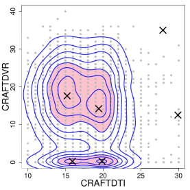
Level sets are regions for which the density value is equal to or above a particular level. Given a level , the -level set (Polonik, 1995; Tsybakov, 1997) is
A natural estimator of is the plug-in estimate from KDE:
The pink area in the right panel of Figure 7 is one instance of the density level set.
There is substantial statistical literature discussing different types of convergence of ; see Polonik (1995); Tsybakov (1997); Rinaldo and Wasserman (2010); Rinaldo et al. (2012) and the references therein. Mammen and Polonik (2013) and Chen et al. (2015c) propose procedures for constructing confidence sets of through bootstrapping the estimator . Note that a visualization tool444R source code: https://github.com/yenchic/HDLV for multivariate level sets is proposed in Chen et al. (2015c).
4.3 Ridges
Another interesting geometric structures are ridges (Genovese et al., 2014; Chen et al., 2015b; Qiao et al., 2016) of the density functions. Formally, ridges are defined as follows. Let be the matrix consisting of the second eigenvector to the last eigenvector. A density ridge is defined as
Intuitively, any point is a local mode in the subspace spanned by . Thus, if we move away from in the subspace, the density value decreases, which is the characteristic attribute of a ridge.
To estimate , we again use the plug-in from KDE:
where and are KDE versions of and respectively. The convergence rate and topological characteristics were discussed in Genovese et al. (2014). Chen et al. (2015b) and Qiao et al. (2016) both studied the asymptotic theory, and Chen et al. (2015b) further proposed methods of constructing confidence sets of . Ozertem and Erdogmus (2011) introduced the subspace-constrained mean shift (SCMS) algorithm to compute . The red curves in the right panel of Figure 7 are estimated ridges from the SCMS algorithm.
4.4 Morse-Smale Complex
The Morse-Smale complex (Banyaga, 2004) of a density function is a partition of the entire support based on the density gradient flow. For any point , we define a gradient ascent flow such that
Namely, is a flow starting at such that we move along the orientation of the density gradient ascent. By Morse theory (Morse, 1925, 1930), such a flow converges to a destination that is one of the critical points (points where ) when the density function is smooth.
Similarly, we define a gradient descent flow such that
In a similar manner to , starts at but now the flow moves by following density gradient descent. Again, by Morse theory, such a flow converges also to one of the critical points, but not to the same point as the destination of . Based on the destinations of and , we partition the entire support into different regions; points within the same region share the same destination for both the gradient ascent flow and the gradient descent flow. This partition is called the Morse-Smale complex.
To estimate the Morse-Smale complex of , we use the Morse-Smale complex of . Arias-Castro et al. (2016) and Chen et al. (2015d) studied the convergence of gradient flows and the Morse-Smale complex of and proved the statistical consistency of these geometric features. Chen et al. (2015d) further proposed to use the Morse-Smale complex to visualize a multivariate density function555R source code: https://github.com/yenchic/Morse_Smale. Note that one can use the R package ‘msr666https://cran.r-project.org/web/packages/msr/index.html’ that to perform data analysis with the Morse-Smale complex (see Gerber et al. (2010); Gerber and Potter (2011); Gerber et al. (2013) for more details).
4.5 Cluster Trees
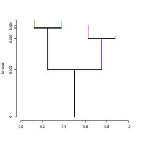
Cluster trees (also known as density trees Stuetzle (2003); Klemelä (2009)) are tree-structured objects summarizing the structure of the underlying density function. The left panel of Figure 8 provides an example of a cluster tree corresponding to KDE in the right panel of Figure 2 (also the same dataset as in Figure 7 and 8). A cluster tree is constructed as follows. Recall that is the density level set at the level . When the level is too large, will be empty, because no region has a density value above such level. When we gradually decrease from a large number, at some levels (when hits the density value of local modes), a new connected component will be created; this corresponds the creation of a connected component. Moreover, at particular levels, two or more connected components will merge (generally at the density value of local minima or saddle points); this corresponds to the elimination of a connected component. Cluster tree uses a tree structure to summarize the creation and elimination of connected components at different levels. Since a cluster tree always live in a 2D plane, it is an excellent tool for visualizing a multivariate density function. For more details, we refer to the review paper in Wasserman (2016).
The above defines a cluster tree using the underlying population density . In practice, we can construct an estimated cluster tree using KDE . Convergence of the cluster tree estimator was studied in Balakrishnan et al. (2013); Chaudhuri et al. (2014); Eldridge et al. (2015); Chen (2016). Jisu et al. (2016) provides a procedure for constructing confidence sets of cluster trees based on bootstrapping KDE . In R, one can use the package ‘TDA777https://cran.r-project.org/web/packages/TDA/index.html’ to construct a tree estimator of KDE.
4.6 Persistent Diagram
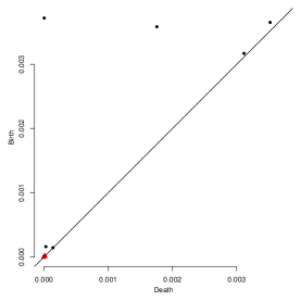
A persistent diagram (Cohen-Steiner et al., 2007; Edelsbrunner and Morozov, 2012; Wasserman, 2016) is a diagram summarizing the topological features of a density function . The construction of a persistent diagram is very similar to that of a cluster tree, but now we focus on not only the connected components but also higher-order topological structures, such as loops and voids (see Fasy et al. (2014); Wasserman (2016) for a more details).
There are several means of estimating a persistent diagram. A natural approach is to use the persistent diagram of KDE . For such an estimator, the stability theorem in Cohen-Steiner et al. (2007) together with the uniform convergence in Section 2.1 are sufficient to prove the convergence of the estimated persistent diagram toward the population persistent diagram. For statistical inference, Fasy et al. (2014) proposes a bootstrap approach over KDE to construct a confidence set. In practice, one can use R package ‘TDA888https://cran.r-project.org/web/packages/TDA/index.html’ to construct the persistent diagram of KDE.
The right panel of Figure 8 shows an example of the persistent diagram of connected components (zeroth-order topological features) and loops (first-order topological features) of KDE described in the right panel of Figure 2. At the top of the figure, the four dots indicate the existence of the four high-density local modes. In the bottom left regions, the black dots and red triangles are the topological noises representing low-density local modes (black dots) and low-density “loops” structures (red triangles; first-order topological features). Note that the two low-density local modes (black crosses) in the right part of both panels of Figure 7 are topological noises corresponding to the two black dots in the bottom left corner of the persistent diagram.
5 Estimating the CDF
KDE can also be used to estimate a CDF (Nadaraya, 1964). The estimator is simple; we just integrate KDE (for simplicity, here we consider the univariate case):
| (17) |
Convergence of such estimators was extensively analyzed soon after their introduction (Winter, 1973; Azzalini, 1981; Reiss, 1981; Fernholz, 1991; Yukich, 1992; Mack, 1984).
Similarly to the pointwise error rate, one can show that
(see the derivation in Nadaraya (1964) and Azzalini (1981)). Again, the first quantity is related to the bias. The other two quantities are related to the stochastic variation. Under such a rate, the optimal smoothing bandwidth will be , which leads to the error rate
the same as using the empirical CDF. Note that as long as , we will obtain the square root error rate.
To construct a confidence band of via , one can use the uniform central limit theorem proposed by Giné and Nickl (2008) to relate the uniform loss to the supremum of a Gaussian process and then use either the limiting distribution or the bootstrap. Note that to apply the result in Giné and Nickl (2008), one have to undersmooth (see Theorem 4 and Section 4.1.1 in Giné and Nickl (2008)) the data or use a higher order kernel function (see Remark 7 and Corollary 2 in Giné and Nickl (2008)).
5.1 ROC Curve
KDE can also be applied to estimate and infer the receiver operating characteristic (ROC) curve (McNeil and Hanley, 1984). In the setting of the ROC curve, we observed two samples. The first is the sample of healthy subjects, whose responses are from an unknown density . The other is the sample of diseased individuals, whose response are from an unknown density . Consider a simple rule of classification based on choosing a cutoff point such that we classify an individual as diseased if its response value is larger than , otherwise it is classified as a healthy individual.
For such a rule, the sensitivity is , the probability of detecting a diseased subject. We also define the specificity , the probability of successfully assigning a healthy subject to the healthy group. Then, the ROC curve is defined as the plotting of the true positive fraction versus the false positive fraction , or equivalently, as plotting the function
A recent review on ROC curves can be found in Demidenko (2012).
A classical nonparametric approach of estimating is to plug-in the empirical CDF estimator for both and (Hsieh et al., 1996). As an alternative, one can use the integrated KDEs of both samples to estimate the ROC curve (Zou et al., 1997; Zhou and Harezlak, 2002; Hall et al., 2004) as equation (17). This is often called a smoothed estimator of the ROC curve because the resulting ROC curve estimator is generally a smooth curve.
To construct confidence bands of an ROC curve, most methods propose using the plug-in estimate from the empirical distribution and constructing the confidence band by the bootstrap (Moise et al., 1985; Campbell, 1994; Macskassy and Provost, 2004). A formal proof of the theoretical validity of such a bootstrap approach is provided in Hall et al. (2004); Horváth et al. (2008); Bertail et al. (2009). Note that can also construct a confidence band by bootstrapping the smoothed ROC curve estimator and using the method proposed in Section 3.2 to construct a confidence band.
6 Conclusion and Open Problems
In this tutorial, we reviewed KDE’s basic properties and its applications in estimating structures of the underlying density function. For readers who would like to learn more about different varieties of KDE, we recommend Wasserman (2006) and Scott (2015). Because this is a tutorial, we ignore many advanced topics such as the minimax theory and adaptation. An introduction of these theoretical properties can be found in Tsybakov (2009).
Although KDE has been widely studied since its introduction in the 1960s, there are still open problems that deserve further investigation. Here we briefly discuss some open problems related to the materials in this tutorial.
-
•
Confidence bands of other KDE-type estimators. In addition to estimating a probability density function and its related structures, the idea of kernel smoothing can be applied to estimate a regression, hazard, or survival function. Moreover, in casual inference, we might be interested in the difference between the regression/hazard/survival function from the control group and that from the treatment group as a characteristic of the treatment effect. One example is the conditional average treatment effect (Lee and Whang, 2009; Hsu, 2013; Ma and Zhou, 2014; Abrevaya et al., 2015). Although in this tutorial we have seen methods of constructing confidence bands of density functions, how to construct a (asymptotically) valid confidence band of these functions remains an open question.
-
•
Multidimensional problems. When the dimension of the data is large, KDE poses several challenges. First, KDE (and most other nonparametric density estimators) suffers severely from the so-called curse of dimensionality: The optimal convergence rate is very slow when is large, and this slow convergence rate cannot be improved (Stone, 1982; Tsybakov, 2009) unless we assume extra smoothness. One way to solve this problem is to find density surrogates that can be estimated easily and to switch our parameter of interest to a density surrogate. However, this rises the question of what the correct surrogates and the corresponding estimators are, and this still remains unclear. Another issue of KDE in multi-dimensions is visualization. When , we can no longer see the entire KDE, and therefore we must use visualization tools to explore our density estimates. However, it is still unclear how to choose a visualization tool in practice.
-
•
More about geometric/topological structures. In Section 4, we saw that several useful geometric and topological structures can be estimated by the corresponding structures of KDE. However, we do not yet fully understand the behavior of these estimators. For instance, how to choose the smoothing bandwidth that optimally estimate these structures is unclear. Handling this issue may require generalizing the concept of the MISE to the set estimator (Chen et al., 2015a) and choosing the smoothing bandwidth that minimizes such an error measurement. In addition to bandwidth selection, uniform inference remains an open question for these structures. Although there are methods of constructing confidence sets of most of these structures, it is unclear whether the resulting confidence sets are uniform for a collection of density functions. Moreover, theoretical optimality, such as the minimax theory, remains unclear for several of these structures, presenting another set of open questions in the study of KDE.
Acknowledgement
We thank two referees for the very useful suggestions. We also thank Gang Chen, Aurelio Uncini, and Larry Wasserman for useful comments.
References
- Abrevaya et al. (2015) J. Abrevaya, Y.-C. Hsu, and R. P. Lieli. Estimating conditional average treatment effects. Journal of Business & Economic Statistics, 33(4):485–505, 2015.
- Arias-Castro et al. (2016) E. Arias-Castro, D. Mason, and B. Pelletier. On the estimation of the gradient lines of a density and the consistency of the mean-shift algorithm. Journal of Machine Learning Research, 17(43):1–28, 2016.
- Azizyan et al. (2015) M. Azizyan, Y.-C. Chen, A. Singh, and L. Wasserman. Risk bounds for mode clustering. arXiv preprint arXiv:1505.00482, 2015.
- Azzalini (1981) A. Azzalini. A note on the estimation of a distribution function and quantiles by a kernel method. Biometrika, pages 326–328, 1981.
- Balakrishnan et al. (2013) S. Balakrishnan, S. Narayanan, A. Rinaldo, A. Singh, and L. Wasserman. Cluster trees on manifolds. In Advances in Neural Information Processing Systems, pages 2679–2687, 2013.
- Banyaga (2004) A. Banyaga. Lectures on Morse homology, volume 29. Springer Science & Business Media, 2004.
- Beekly et al. (2007) D. L. Beekly, E. M. Ramos, W. W. Lee, W. D. Deitrich, M. E. Jacka, J. Wu, J. L. Hubbard, T. D. Koepsell, J. C. Morris, W. A. Kukull, et al. The national alzheimer’s coordinating center (nacc) database: the uniform data set. Alzheimer Disease & Associated Disorders, 21(3):249–258, 2007.
- Beran (1987) R. Beran. Prepivoting to reduce level error of confidence sets. Biometrika, 74(3):457–468, 1987.
- Bertail et al. (2009) P. Bertail, S. J. Clémençcon, and N. Vayatis. On bootstrapping the roc curve. In Advances in Neural Information Processing Systems, pages 137–144, 2009.
- Bickel and Rosenblatt (1973) P. Bickel and M. Rosenblatt. On some global measures of the deviations of density function estimates. The Annals of Statistics, 1(6):1071–1095, 1973.
- Bjerve et al. (1985) S. Bjerve, K. A. Doksum, and B. S. Yandell. Uniform confidence bounds for regression based on a simple moving average. Scandinavian Journal of Statistics, pages 159–169, 1985.
- Bowman (1984) A. Bowman. An alternative method of cross-validation for the smoothing of density estimates. Biometrika, 71(2):353–360, 1984.
- Bowman and Azzalini (1997) A. W. Bowman and A. Azzalini. Applied smoothing techniques for data analysis: the kernel approach with S-Plus illustrations, volume 18. OUP Oxford, 1997.
- Breiman et al. (1977) L. Breiman, W. Meisel, and E. Purcell. Variable kernel estimates of multivariate densities. Technometrics, 19(2):135–144, 1977.
- Calonico et al. (2015) S. Calonico, M. D. Cattaneo, and M. H. Farrell. On the effect of bias estimation on coverage accuracy in nonparametric inference. arXiv preprint arXiv:1508.02973, 2015.
- Campbell (1994) G. Campbell. Advances in statistical methodology for the evaluation of diagnostic and laboratory tests. Statistics in medicine, 13(5-7):499–508, 1994.
- Chacón and Duong (2013) J. E. Chacón and T. Duong. Data-driven density derivative estimation, with applications to nonparametric clustering and bump hunting. Electronic Journal of Statistics, 7:499–532, 2013.
- Chacón et al. (2011) J. E. Chacón, T. Duong, and M. Wand. Asymptotics for general multivariate kernel density derivative estimators. Statistica Sinica, 21:807–840, 2011.
- Chacón et al. (2015) J. E. Chacón et al. A population background for nonparametric density-based clustering. Statistical Science, 30(4):518–532, 2015.
- Chaudhuri et al. (2014) K. Chaudhuri, S. Dasgupta, S. Kpotufe, and U. von Luxburg. Consistent procedures for cluster tree estimation and pruning. IEEE Transactions on Information Theory, 60(12):7900–7912, 2014.
- Chazal et al. (2014) F. Chazal, B. T. Fasy, F. Lecci, B. Michel, A. Rinaldo, and L. Wasserman. Robust topological inference: Distance to a measure and kernel distance. arXiv preprint arXiv:1412.7197, 2014.
- Chen (1996) S. X. Chen. Empirical likelihood confidence intervals for nonparametric density estimation. Biometrika, 83(2):329–341, 1996.
- Chen and Qin (2002) S. X. Chen and Y. S. Qin. Confidence intervals based on local linear smoother. Scandinavian Journal of Statistics, 29(1):89–99, 2002.
- Chen (2016) Y.-C. Chen. Generalized cluster trees and singular measures. arXiv preprint arXiv:1611.02762, 2016.
- Chen (2017) Y.-C. Chen. Nonparametric inference via bootstrapping the debiased estimator. arXiv preprint arXiv:1702.07027, 2017.
- Chen et al. (2015a) Y.-C. Chen, C. R. Genovese, S. Ho, and L. Wasserman. Optimal ridge detection using coverage risk. In Advances in Neural Information Processing Systems, pages 316–324, 2015a.
- Chen et al. (2015b) Y.-C. Chen, C. R. Genovese, and L. Wasserman. Asymptotic theory for density ridges. The Annals of Statistics, 43(5):1896–1928, 2015b.
- Chen et al. (2015c) Y.-C. Chen, C. R. Genovese, and L. Wasserman. Density level sets: Asymptotics, inference, and visualization. arXiv:1504.05438, 2015c.
- Chen et al. (2015d) Y.-C. Chen, C. R. Genovese, and L. Wasserman. Statistical inference using the morse-smale complex. arXiv preprint arXiv:1506.08826, 2015d.
- Chen et al. (2016) Y.-C. Chen, C. R. Genovese, and L. Wasserman. A comprehensive approach to mode clustering. Electronic Journal of Statistics, 10(1):210–241, 2016.
- Cheng (1995) Y. Cheng. Mean shift, mode seeking, and clustering. Pattern Analysis and Machine Intelligence, IEEE Transactions on, 17(8):790–799, 1995.
- Chernozhukov et al. (2013) V. Chernozhukov, D. Chetverikov, and K. Kato. Gaussian approximations and multiplier bootstrap for maxima of sums of high-dimensional random vectors. The Annals of Statistics, 41(6):2786–2819, 2013.
- Chernozhukov et al. (2014a) V. Chernozhukov, D. Chetverikov, and K. Kato. Anti-concentration and honest, adaptive confidence bands. The Annals of Statistics, 42(5):1787–1818, 2014a.
- Chernozhukov et al. (2014b) V. Chernozhukov, D. Chetverikov, and K. Kato. Comparison and anti-concentration bounds for maxima of gaussian random vectors. Probability Theory and Related Fields, pages 1–24, 2014b.
- Chernozhukov et al. (2014c) V. Chernozhukov, D. Chetverikov, and K. Kato. Gaussian approximation of suprema of empirical processes. The Annals of Statistics, 42(4):1564–1597, 2014c.
- Chernozhukov et al. (2016) V. Chernozhukov, D. Chetverikov, and K. Kato. Empirical and multiplier bootstraps for suprema of empirical processes of increasing complexity, and related gaussian couplings. Stochastic Processes and their Applications, 2016.
- Cohen-Steiner et al. (2007) D. Cohen-Steiner, H. Edelsbrunner, and J. Harer. Stability of persistence diagrams. Discrete & Computational Geometry, 37(1):103–120, 2007.
- Comaniciu and Meer (2002) D. Comaniciu and P. Meer. Mean shift: A robust approach toward feature space analysis. Pattern Analysis and Machine Intelligence, IEEE Transactions on, 24(5):603–619, 2002.
- Demidenko (2012) E. Demidenko. Confidence intervals and bands for the binormal roc curve revisited. Journal of applied statistics, 39(1):67–79, 2012.
- Deng and Wickham (2011) H. Deng and H. Wickham. Density estimation in r. http://vita.had.co.nz/papers/density-estimation.pdf, 2011.
- Edelsbrunner and Morozov (2012) H. Edelsbrunner and D. Morozov. Persistent homology: theory and practice. In Proceedings of the European Congress of Mathematics, pages 31–50, 2012.
- Efron (1979) B. Efron. Bootstrap methods: Another look at the jackknife. Annals of Statistics, 7(1):1–26, 1979.
- Einmahl and Mason (2005) U. Einmahl and D. M. Mason. Uniform in bandwidth consistency of kernel-type function estimators. The Annals of Statistics, 33(3):1380–1403, 2005.
- Eldridge et al. (2015) J. Eldridge, M. Belkin, and Y. Wang. Beyond hartigan consistency: Merge distortion metric for hierarchical clustering. In Proceedings of The 28th Conference on Learning Theory, pages 588–606, 2015.
- Eubank and Speckman (1993) R. L. Eubank and P. L. Speckman. Confidence bands in nonparametric regression. Journal of the American Statistical Association, 88(424):1287–1301, 1993.
- Fasy et al. (2014) B. T. Fasy, F. Lecci, A. Rinaldo, L. Wasserman, S. Balakrishnan, and A. Singh. Confidence sets for persistence diagrams. The Annals of Statistics, 42(6):2301–2339, 2014.
- Fernholz (1991) L. T. Fernholz. Almost sure convergence of smoothed empirical distribution functions. Scandinavian Journal of Statistics, pages 255–262, 1991.
- Fukunaga and Hostetler (1975) K. Fukunaga and L. Hostetler. The estimation of the gradient of a density function, with applications in pattern recognition. Information Theory, IEEE Transactions on, 21(1):32–40, 1975.
- Genovese et al. (2009) C. R. Genovese, M. Perone-Pacifico, I. Verdinelli, and L. Wasserman. On the path density of a gradient field. The Annals of Statistics, 37(6A):3236–3271, 2009.
- Genovese et al. (2014) C. R. Genovese, M. Perone-Pacifico, I. Verdinelli, and L. Wasserman. Nonparametric ridge estimation. The Annals of Statistics, 42(4):1511–1545, 2014.
- Gerber and Potter (2011) S. Gerber and K. Potter. Data analysis with the morse-smale complex: The msr package for r. Journal of Statistical Software, 2011.
- Gerber et al. (2010) S. Gerber, P.-T. Bremer, V. Pascucci, and R. Whitaker. Visual exploration of high dimensional scalar functions. Visualization and Computer Graphics, IEEE Transactions on, 16(6):1271–1280, 2010.
- Gerber et al. (2013) S. Gerber, O. Rübel, P.-T. Bremer, V. Pascucci, and R. T. Whitaker. Morse–smale regression. Journal of Computational and Graphical Statistics, 22(1):193–214, 2013.
- Giné and Guillou (2002) E. Giné and A. Guillou. Rates of strong uniform consistency for multivariate kernel density estimators. In Annales de l’Institut Henri Poincare (B) Probability and Statistics, volume 38, pages 907–921. Elsevier, 2002.
- Giné and Nickl (2008) E. Giné and R. Nickl. Uniform central limit theorems for kernel density estimators. Probability Theory and Related Fields, 141(3-4):333–387, 2008.
- Goldenshluger and Lepski (2008) A. Goldenshluger and O. Lepski. Universal pointwise selection rule in multivariate function estimation. Bernoulli, 14(4):1150–1190, 2008.
- Goldenshluger and Lepski (2011) A. Goldenshluger and O. Lepski. Bandwidth selection in kernel density estimation: Oracle inequalities and adaptive minimax optimality. The Annals of Statistics, 39(3):1608–1632, 2011.
- Hall (1986) P. Hall. On the bootstrap and confidence intervals. The Annals of Statistics, 14(4):1431–1452, 1986.
- Hall (1991) P. Hall. On convergence rates of suprema. Probability Theory and Related Fields, 89(4):447–455, 1991.
- Hall (1992a) P. Hall. On bootstrap confidence intervals in nonparametric regression. The Annals of Statistics, 20(2):695–711, 1992a.
- Hall (1992b) P. Hall. Effect of bias estimation on coverage accuracy of bootstrap confidence intervals for a probability density. The Annals of Statistics, 20(2):675–694, 1992b.
- Hall and Horowitz (2013) P. Hall and J. Horowitz. A simple bootstrap method for constructing nonparametric confidence bands for functions. The Annals of Statistics, 41(4):1892–1921, 2013.
- Hall and Owen (1993) P. Hall and A. B. Owen. Empirical likelihood confidence bands in density estimation. Journal of Computational and Graphical Statistics, 2(3):273–289, 1993.
- Hall et al. (2004) P. Hall, R. J. Hyndman, and Y. Fan. Nonparametric confidence intervals for receiver operating characteristic curves. Biometrika, 91(3):743–750, 2004.
- Härdle and Bowman (1988) W. Härdle and A. W. Bowman. Bootstrapping in nonparametric regression: local adaptive smoothing and confidence bands. Journal of the American Statistical Association, 83(401):102–110, 1988.
- Hardle and Marron (1991) W. Hardle and J. Marron. Bootstrap simultaneous error bars for nonparametric regression. The Annals of Statistics, 19(2):778–796, 1991.
- Härdle et al. (1995) W. Härdle, S. Huet, and E. Jolivet. Better bootstrap confidence intervals for regression curve estimation. Statistics: A Journal of Theoretical and Applied Statistics, 26(4):287–306, 1995.
- Härdle et al. (2004) W. Härdle, S. Huet, E. Mammen, and S. Sperlich. Bootstrap inference in semiparametric generalized additive models. Econometric Theory, 20(02):265–300, 2004.
- Horváth et al. (2008) L. Horváth, Z. Horváth, and W. Zhou. Confidence bands for roc curves. Journal of Statistical Planning and Inference, 138(6):1894–1904, 2008.
- Hsieh et al. (1996) F. Hsieh, B. W. Turnbull, et al. Nonparametric and semiparametric estimation of the receiver operating characteristic curve. The annals of statistics, 24(1):25–40, 1996.
- Hsu (2013) Y.-C. Hsu. Consistent tests for conditional treatment effects. Technical report, Institute of Economics, Academia Sinica, Taipei, Taiwan, 2013.
- Jisu et al. (2016) K. Jisu, Y.-C. Chen, S. Balakrishnan, A. Rinaldo, and L. Wasserman. Statistical inference for cluster trees. In Advances In Neural Information Processing Systems, pages 1831–1839, 2016.
- Jones et al. (1996) M. C. Jones, J. S. Marron, and S. J. Sheather. A brief survey of bandwidth selection for density estimation. Journal of the American Statistical Association, 91(433):401–407, 1996.
- Klemelä (2009) J. Klemelä. Smoothing of multivariate data: density estimation and visualization, volume 737. John Wiley & Sons, 2009.
- Lee and Whang (2009) S. Lee and Y.-J. Whang. Nonparametric tests of conditional treatment effects. 2009.
- Lepski and Goldenshluger (2009) O. Lepski and A. Goldenshluger. Structural adaptation via lp-norm oracle inequalities. Probab. Theory Related Fields, 126(1-2):47–71, 2009.
- Loftsgaarden and Quesenberry (1965) D. O. Loftsgaarden and C. P. Quesenberry. A nonparametric estimate of a multivariate density function. The Annals of Mathematical Statistics, 36(3):1049–1051, 1965.
- Loh (1987) W.-Y. Loh. Calibrating confidence coefficients. Journal of the American Statistical Association, 82(397):155–162, 1987.
- Ma and Zhou (2014) Y. Ma and X.-H. Zhou. Treatment selection in a randomized clinical trial via covariate-specific treatment effect curves. Statistical methods in medical research, page 0962280214541724, 2014.
- Mack (1984) Y. Mack. Remarks on some smoothed empirical distribution functions and process. Bulletin of informatics and cybernetics, 21(1/2):29–35, 1984.
- Macskassy and Provost (2004) S. Macskassy and F. Provost. Confidence bands for roc curves: Methods and an empirical study. Proceedings of the First Workshop on ROC Analysis in AI. August 2004., 2004.
- Mammen and Polonik (2013) E. Mammen and W. Polonik. Confidence regions for level sets. Journal of Multivariate Analysis, 122:202–214, 2013.
- McMurry and Politis (2008) T. L. McMurry and D. N. Politis. Bootstrap confidence intervals in nonparametric regression with built-in bias correction. Statistics & Probability Letters, 78(15):2463–2469, 2008.
- McNeil and Hanley (1984) B. J. McNeil and J. A. Hanley. Statistical approaches to the analysis of receiver operating characteristic (roc) curves. Medical decision making, 4(2):137–150, 1984.
- Moise et al. (1985) A. Moise, B. Clément, P. Ducimetière, and M. G. Bourassa. Comparison of receiver operating curves derived from the same population: a bootstrapping approach. Computers and biomedical research, 18(2):125–131, 1985.
- Morse (1925) M. Morse. Relations between the critical points of a real function of n independent variables. Transactions of the American Mathematical Society, 27(3):345–396, 1925.
- Morse (1930) M. Morse. The foundations of a theory of the calculus of variations in the large in m-space (second paper). Transactions of the American Mathematical Society, 32(4):599–631, 1930.
- Nadaraya (1964) E. A. Nadaraya. Some new estimates for distribution functions. Theory of Probability & Its Applications, 9(3):497–500, 1964.
- Neumann (1995) M. H. Neumann. Automatic bandwidth choice and confidence intervals in nonparametric regression. The Annals of Statistics, 23(6):1937–1959, 1995.
- Neumann (1998) M. H. Neumann. Strong approximation of density estimators from weakly dependent observations by density estimators from independent observations. Annals of Statistics, pages 2014–2048, 1998.
- Neumann and Polzehl (1998) M. H. Neumann and J. Polzehl. Simultaneous bootstrap confidence bands in nonparametric regression. Journal of Nonparametric Statistics, 9(4):307–333, 1998.
- Ozertem and Erdogmus (2011) U. Ozertem and D. Erdogmus. Locally defined principal curves and surfaces. Journal of Machine Learning Research, 2011.
- Parzen (1962) E. Parzen. On estimation of a probability density function and mode. The Annals of Mathematical Statistics, 33(3):1065–1076, 1962.
- Polonik (1995) W. Polonik. Measuring mass concentrations and estimating density contour clusters-an excess mass approach. The Annals of Statistics, pages 855–881, 1995.
- Qiao et al. (2016) W. Qiao, W. Polonik, et al. Theoretical analysis of nonparametric filament estimation. The Annals of Statistics, 44(3):1269–1297, 2016.
- Rao (2014) B. P. Rao. Nonparametric functional estimation. Academic press, 2014.
- Reiss (1981) R.-D. Reiss. Nonparametric estimation of smooth distribution functions. Scandinavian Journal of Statistics, pages 116–119, 1981.
- Rinaldo and Wasserman (2010) A. Rinaldo and L. Wasserman. Generalized density clustering. The Annals of Statistics, 38(5):2678–2722, 2010.
- Rinaldo et al. (2012) A. Rinaldo, A. Singh, R. Nugent, and L. Wasserman. Stability of density-based clustering. The Journal of Machine Learning Research, 13(1):905–948, 2012.
- Romano (1988a) J. P. Romano. Bootstrapping the mode. Annals of the Institute of Statistical Mathematics, 40(3):565–586, 1988a.
- Romano (1988b) J. P. Romano. On weak convergence and optimality of kernel density estimates of the mode. The Annals of Statistics, pages 629–647, 1988b.
- Rosenblatt et al. (1976) M. Rosenblatt et al. On the maximal deviation of -dimensional density estimates. The Annals of Probability, 4(6):1009–1015, 1976.
- Rudemo (1982) M. Rudemo. Empirical choice of histograms and kernel density estimators. Scandinavian Journal of Statistics, pages 65–78, 1982.
- Scott (2015) D. W. Scott. Multivariate density estimation: theory, practice, and visualization. John Wiley & Sons, 2015.
- Scott and Terrell (1987) D. W. Scott and G. R. Terrell. Biased and unbiased cross-validation in density estimation. Journal of the american Statistical association, 82(400):1131–1146, 1987.
- Sheather and Jones (1991) S. Sheather and C. Jones. A reliable data-based bandwidth selection method for kernel density estimation. Journal of the Royal Statistical Society: Series B (Statistical Methodology), 53(3):683–690, 1991.
- Sheather (2004) S. J. Sheather. Density estimation. Statistical Science, 19(4):588–597, 2004.
- Silverman (1986) B. W. Silverman. Density Estimation for Statistics and Data Analysis. Chapman and Hall, 1986.
- Stoker (1993) T. M. Stoker. Smoothing bias in density derivative estimation. Journal of the American Statistical Association, 88(423):855–863, 1993.
- Stone (1982) C. J. Stone. Optimal global rates of convergence for nonparametric regression. The Annals of Statistics, 10(4):1040–1053, 1982.
- Stone (1984) C. J. Stone. An asymptotically optimal window selection rule for kernel density estimates. The Annals of Statistics, 12(4):1285–1297, 1984.
- Stuetzle (2003) W. Stuetzle. Estimating the cluster tree of a density by analyzing the minimal spanning tree of a sample. Journal of classification, 20(1):025–047, 2003.
- Sun and Loader (1994) J. Sun and C. R. Loader. Simultaneous confidence bands for linear regression and smoothing. The Annals of Statistics, 22(3):1328–1345, 1994.
- Terrell and Scott (1992) G. R. Terrell and D. W. Scott. Variable kernel density estimation. The Annals of Statistics, 20(3):1236–1265, 1992.
- Tsybakov (1997) A. B. Tsybakov. On nonparametric estimation of density level sets. The Annals of Statistics, 25(3):948–969, 1997.
- Tsybakov (2009) A. B. Tsybakov. Introduction to nonparametric estimation. revised and extended from the 2004 french original. translated by vladimir zaiats, 2009.
- Wasserman (2006) L. Wasserman. All of Nonparametric Statistics. Springer-Verlag New York, Inc., 2006.
- Wasserman (2016) L. Wasserman. Topological data analysis. arXiv preprint arXiv:1609.08227, 2016.
- Winter (1973) B. Winter. Strong uniform consistency of integrals of density estimators. Canadian Journal of Statistics, 1(1-2):247–253, 1973.
- Woodroofe (1970) M. Woodroofe. On choosing a delta-sequence. The Annals of Mathematical Statistics, 41(5):1665–1671, 1970.
- Xia (1998) Y. Xia. Bias-corrected confidence bands in nonparametric regression. Journal of the Royal Statistical Society: Series B (Statistical Methodology), 60(4):797–811, 1998.
- Yukich (1985) J. Yukich. Laws of large numbers for classes of functions. Journal of multivariate analysis, 17(3):245–260, 1985.
- Yukich (1992) J. Yukich. Weak convergence of smoothed empirical processes. Scandinavian journal of statistics, pages 271–279, 1992.
- Zhou and Harezlak (2002) X.-H. Zhou and J. Harezlak. Comparison of bandwidth selection methods for kernel smoothing of roc curves. Statistics in medicine, 21(14):2045–2055, 2002.
- Zou et al. (1997) K. H. Zou, W. Hall, and D. E. Shapiro. Smooth non-parametric receiver operating characteristic (roc) curves for continuous diagnostic tests. Statistics in medicine, 16(19):2143–2156, 1997.
See pages - of PDF/R_code