Fitting Analysis using Differential Evolution Optimization (fado):

The goal of population spectral synthesis (pss; also referred to as inverse, semi-empirical evolutionary- or fossil record approach) is to decipher from the spectrum of a galaxy the mass, age and metallicity of its constituent stellar populations. This technique, which is the reverse of but complementary to evolutionary synthesis, has been established as fundamental tool in extragalactic research. It has been extensively applied to large spectroscopic data sets, notably the SDSS, leading to important insights into the galaxy assembly history. However, despite significant improvements over the past decade, all current pss codes suffer from two major deficiencies that inhibit us from gaining sharp insights into the star-formation history (SFH) of galaxies and potentially introduce substantial biases in studies of their physical properties (e.g., stellar mass, mass-weighted stellar age and specific star formation rate). These are i) the neglect of nebular emission in spectral fits, consequently, ii) the lack of a mechanism that ensures consistency between the best-fitting SFH and the observed nebular emission characteristics of a star-forming (SF) galaxy (e.g., hydrogen Balmer-line luminosities and equivalent widths-EWs, shape of the continuum in the region around the Balmer and Paschen jump). In this article, we present fado (Fitting Analysis using Differential evolution Optimization) – a conceptually novel, publicly available pss tool with the distinctive capability of permitting identification of the SFH that reproduces the observed nebular characteristics of a SF galaxy. This so-far unique self-consistency concept allows us to significantly alleviate degeneracies in current spectral synthesis, thereby opening a new avenue to the exploration of the assembly history of galaxies. The innovative character of fado is further augmented by its mathematical foundation: fado is the first pss code employing genetic differential evolution optimization. This, in conjunction with various other currently unique elements in its mathematical concept and numerical realization (e.g., mid-analysis optimization of the spectral library using artificial intelligence, test for convergence through a procedure inspired by Markov chain Monte Carlo techniques, quasi-parallelization embedded within a modular architecture) results in key improvements with respect to computational efficiency and uniqueness of the best-fitting SFHs. Furthermore, fado incorporates within a single code the entire chain of pre-processing, modeling, post-processing, storage and graphical representation of the relevant output from pss, including emission-line measurements and estimates of uncertainties for all primary and secondary products from spectral synthesis (e.g., mass contributions of individual stellar populations, mass- and luminosity-weighted stellar ages and metallicities). This integrated concept greatly simplifies and accelerates a lengthy sequence of individual time-consuming steps that are generally involved in pss modeling, further enhancing the overall efficiency of the code and inviting to its automated application to large spectroscopic data sets.

1 Introduction

Understanding the formation and evolution of galaxies is undoubtedly one of the greatest challenges of modern astronomy. Excluding the few systems in our close vicinity that can be resolved into individual stars and studied through color-magnitude diagrams, the star-formation history (SFH) of galaxies can only be inferred from spectra, each typically containing the luminosity-weighted output from millions of stars. Deciphering from a spectrum the SFH and chemical enrichment history (CEH) of a galaxy is the objective of spectral synthesis - one of the most computationally demanding yet fundamental tools of extragalactic research. Spectral synthesis comes essentially in two reverse yet complementary techniques – evolutionary and population synthesis (also referred to as inverse, semi-empirical evolutionary- or fossil record approach), inspired, respectively, by the seminal works by Struck-Marcell & Tinsley (1967) and Faber (1972).

The goal of evolutionary spectral synthesis (ess) is to compute the time evolution of the spectral energy distribution (SED) of a galaxy on the basis of an assumed SFH and CEH. Comparison of synthetic with observed SEDs permits us to place constraints on the galaxy assembly history (for example, disentangle a quasi-monolithic from a continuous formation process). The fact that the SFH is, by definition, an input quantity to ess facilitates straight-forward predictions of the time evolution of various observables of interest (e.g., colors, hydrogen Balmer-line equivalent widths) and eases a detailed treatment of relevant processes contributing to a galaxy SED (e.g., reprocessing of the ionizing photon output from OB stars into nebular emission for various assumptions on the chemistry, geometry and physical conditions of the gas component). Indeed, starting from the pioneering work by Struck-Marcell & Tinsley (1967), ess underwent several important refinements that permitted nearly panchromatic predictions of the spectrophotometric evolution of galaxies, notably the chemically consistent treatment of gas and stars, and the inclusion of nebular and dust emission in several codes (e.g., Leitherer & Heckman, 1995; Krüger et al., 1995; Fioc & Rocca-Volmerange, 1997; Silva et al., 1998; Leitherer et al., 1999; Fioc & Rocca-Volmerange, 1999; Kewley et al., 2001; Charlot & Longhetti, 2001; Zackrisson et al., 2001; Anders & Fritze von Alvensleben, 2003; Anders et al., 2004; Groves et al., 2008; Zackrisson et al., 2008; Kotulla et al., 2009; Schaerer & de Barros, 2009; Verhamme, 2012; Mollá et al., 2009; Martín-Manjón et al., 2010, among others; see Tinsley 1980 and, recently, Conroy 2013 for reviews on the subject) and facilitating different SED fitting tools that include stellar & nebular emission (e.g., Burgarela, Buat & Iglesias-Páramo, 2005; Serra et al., 2011; Acquaviva, Gawieser & Guaita, 2011; Pacifici et al., 2012; Amorín et al., 2012a; Hahn & Hahn, 2014; Chevallard & Charlot, 2016; Leja et al., 2016). Such ess models and the fitting tools built upon them have been extensively applied to the interpretation of galaxy observations (e.g., Guseva et al., 2001; Moy et al., 2001; Guseva et al., 2007; Cairós et al., 2009; Moustakas et al., 2010; Izotov et al., 2011; Amorín et al., 2012a; Schaerer, de Barros & Sklias, 2013; Brinchmann et al., 2013; Maseda et al., 2014; Pacifici et al., 2015; Rodríguez-Muñoz et al., 2015; van der Wel et al., 2016; Izotov et al., 2016).

In the past decade, ess saw impressive advances with regard to the sophistication and complexity of input SFHs&CEHs. Following the early era of $\chi^{2}$-based searches among a limited set of SEDs corresponding to a few simple SFH parametrizations (e.g., continuous star formation at a constant star-formation rate-SFR or exponentially declining SFR with an e-folding timescale between 0.1 and 10 Gyr), several modern variants of ess exploit Bayesian or Markov chain Monte Carlo techniques to search within a set of mock SEDs for the one giving the best match to observations, while additionally providing the posterior probability distribution of various non-linearly coupled evolutionary ingredients. For example, Pacifici et al. (2012) employ a Bayesian approach to a dense grid of pre-computed SEDs, whereas in the models by both Chevallard & Charlot (2016) and Leja et al. (2016) synthetic SEDs are computed on the fly. Approaches taken in computing SED grids include, for example, Monte Carlo realizations of parametric SFHs with random bursts optionally added (e.g., Kauffmann et al., 2003a, b, c; Tremonti et al., 2004; Brinchmann et al., 2004; da Cunha, Charlot & Elbaz, 2008), purely non-parametric SFHs (and CEHs) adopted from post-treatment of cosmological simulations (e.g., Pacifici et al., 2012, 2016, see also De Lucia & Blaizot 2007), or combinations thereof in various spectral fitting tools geared toward multi-band photometry and spectroscopy (e.g., Acquaviva, Gawieser & Guaita, 2011; Pacifici et al., 2012; Hahn & Hahn, 2014; Chevallard & Charlot, 2016; Leja et al., 2016). The trial SEDs used by many of these advanced spectral fitting codes (e.g., Brinchmann et al., 2004; Acquaviva, Gawieser & Guaita, 2011; Pacifici et al., 2012; Chevallard & Charlot, 2016) consistently take into account the nebular emission expected from the Lyman continuum (LyC) photon rate from OB stars, reaching in some cases (e.g., Chevallard & Charlot, 2016) a significant degree of sophistication in the treatment of nebular physics (with, e.g., gas ionization parameter, metallicity and dust-to-metal mass ratio being adjustable input parameters) through coupling of ess with refined photoionization codes (e.g., CLOUDY; Ferland et al., 2013). Indeed, the relatively simple ”forward” physical concept of ess – in essence, SFH-weighted convolution of simple stellar population (SSP) spectra – greatly simplifies inclusion in synthetic SEDs of the post-processed stellar radiation by gas and dust, at the price of ad hoc or semi-empirically founded assumptions on the SFH and CEH of galaxies. Clearly, an important virtue of such coupled ess+photoionization codes is the implicit consistency between the stellar LyC photon output and the predicted Balmer-line luminosities, given that the former is used for the computation of the latter. It should be born in mind, however, that consistency between observed and predicted nebular emission in this case does not imply that the full set of evolutionary and physical characteristics of the stellar component of the best-fitting mock SED (i.e., age and metallicity) are inferred self-consistently, taking into account the observed nebular characteristics, within a multi-dimensional topology of non-linearly coupled parameters.

Summarizing, the SFH – regardless of whether it is entered in a parametric or non-parametric form – remains the main input assumption in current ess models and SED-fitting tools built upon them. The same applies to the CEH: for instance, a best-fitting SED with fixed stellar metallicity $Z$ encapsulates in itself a strong assumption on the CEH of a galaxy (no chemical evolution of stars and gas, in contrast to the chemically consistent evolutionary approach). The benefits from consistent inclusion of nebular emission in chemically inconsistent SED templates might be a subject of debate, given the strong dependence of the LyC photon rate on $Z$. For instance, the H$\alpha$ luminosity expected for a Salpeter initial mass function (IMF) increases from 2$\cdot$$Z_{\odot}$ to $Z_{\odot}$/20 by a factor of approximately four (see e.g., Weilbacher & Fritze-v.Alvensleben, 2001, and references therein), which is certainly of relevance both to SED fitting and SFR determinations of chemically evolving galaxies across cosmic time.

Conversely, the goal of population spectral synthesis (pss, see Walcher et al., 2011, for a review) is to decompose the observed spectrum of a galaxy into its elementary and no further divisible constituents. These are spectra of individual stars or SSPs (spectral snapshots of instantaneously formed stellar populations being fully characterized by their age $t$, chemical composition and initial mass function) that a pss code selects from a spectral base library. The best-fitting solution is an array holding the mass fractions $\mu_{j}$ of the SSP ”building blocks” picked up from the library and is referred to as population vector (PV). The array $\mu_{j}$(SSP($t$,$Z$)) obviously yields a discretized approximation to the SFH and CEH of a galaxy. From the seminal work of Faber (1972) and the remarks above it is apparent that pss is a spectral decomposition (aposynthesis) technique, and inverse to ess (synthesis). Quite importantly, the only condition in this ”mathematical optimization exercise” is that the $\mu_{j}$ elements composing the best-fitting PV are positive and finite. In particular, pss is by definition irreconcilable with any prior or implicit assumption on the SFH and CEH: even a simple functional relation binding two SSPs of different age (or $Z$) into one single ”SFH block” would be equivalent to an implicit assumption on the SFH (or CEH), and would thus violate the principles of pss. The ”inverse” approach of pss obviously also entails a different mathematical concept than that of ”forward computing” ess codes, and makes inclusion and, the more so, consistent treatment, of nebular emission a challenging task within the mathematical/numerical domain of multi-objective optimization (cf. Sect. 3). Finally, given the considerable confusion in the nomenclature (with several cases in the literature citing the term ess and pss interchangeably, or associating pss with ess codes using non-parametric input SFHs/CEHs) it is useful to bear in mind that the term ”parametric” or ”non-parametric” is strictly speaking inapplicable to pss, since the SFH and CEH are not input parameters.

The past decade saw the development of different pss codes, each conceived with a different priority in mind, such as MOPED (Heavens, Jimenez & Lahav, 2000), pPXF (Cappellari & Emesellem, 2004), Starlight (Cid Fernandes et al., 2005; López Fernández et al., 2016) and STECKMAP (Ocvirk et al., 2006). UlySS (Koleva et al., 2009) might be regarded as a special case, since its mathematical concept complies with pss, however, assumptions are imposed on the best-fitting SFH and CEH. For instance, the goal of MOPED is to collapse a galaxy spectrum into its most robust and characteristic spectroscopic features, whereas ULySS and STECKMAP are primarily intended to spectral fitting and kinematical analyses. Starlight, on the other hand, may arguably be regarded as the most intensively applied pss code for the exploration of the SFH of galaxies on the basis of large spectroscopic data sets (e.g., the SDSS, York et al., 2000).

However, despite conceptual and numerical improvements, all currently available pss codes suffer from two important deficiencies that limit their potential for gaining sharp insights into the galaxy assembly history. The first one stems from the notorious SFH – extinction – metallicity degeneracy (e.g., O’Connell, 1996; Pelat, 1997, 1998) and the second one, as we argue next, from the neglect of nebular emission in spectral fits. A direct consequence from the second is obviously the lack of a mechanism that ensures consistency between the best-fitting PV and the observed nebular emission (ne) characteristics in a galaxy, as for example the luminosities and equivalent widths (EWs) of Balmer recombination lines, and the SED characteristics in the spectral region around the Balmer and Paschen jump (3646Å and 8207Å, respectively).

a) Degeneracy of spectral fits: A well known yet far from overcome problem in spectral synthesis (both to pss and to ess) is that an irreproachable fit is in itself no proof neither for the uniqueness nor astrophysical soundness of the best-fitting model: in fact, substantially different PVs, composed of SSPs with different age and $Z_{\star}$, and subjected to different amounts of intrinsic extinction can result in almost indistinguishable SEDs (see, e.g., Guseva et al., 2001, hereafter G01, for a related discussion in the case of grid-based SED-fitting ess tools).

This is specially relevant to studies of star-forming galaxies, where the imprints of, for example, a small (2–5%) mass fraction of instantaneously formed young ionizing stars on the optical continuum can readily be reproduced by a slightly older episode of prolonged star formation without any appreciable young ionizing stellar component (cf. G01). Such degeneracies in the PV may translate into substantial (20-50%) uncertainties in the burst parameter b, propagating then into other quantities of interest, such as the specific SFR (sSFR).

More generally, as shown by an examination of this issue by G01, the uniqueness of spectral fits for star-forming galaxies can hardly be established from $\chi^{2}$-minimization techniques to the optical continuum alone, that is without additional constraints (e.g., EWs of Balmer absorption and emission lines). The degeneracy problem is probably further aggravated by various technical specifics of the fitting procedure (e.g., spectral range considered, quality of the kinematical fitting of stellar absorption features, construction of the SSP library; cf Appendix) the combined effect of which on pss modeling has not been conclusively investigated as yet, even though pilot attempts in this direction exist (see, e.g., Gomes, 2005, 2009; Chen et al., 2010; Richards et al., 2009; Cid Fernandes et al., 2014; Magris et al., 2015, Cardoso, Gomes & Papaderos, in prep., hereafter CGP17).

b) Neglect of nebular emission: A fundamental conceptual shortcoming of all state-of-the-art pss codes is the neglect of ne. First, ne, as natural consequence of star formation is inseparable from the galaxy assembly process and an indispensable ingredient of any physically meaningful spectral model (e.g., Grewing, Demoulin & Burbidge, 1968; Huchra, 1977; Leitherer & Heckman, 1995; Krüger et al., 1995). In particular, inclusion of ne is crucial to the pss modeling of intermediate-to-high $z$ galaxies, where intense SF activity is virtually omnipresent. According to our current knowledge, these systems are building up their stellar component through starbursts or prolonged episodes of strongly elevated sSFR, translating into short (a few $10^{8}$ yr) stellar mass (${\cal M}_{\star}$) doubling times. The ionizing output from massive young stars, forming at prodigious rates during such dominant phases of galaxy buildup is plausibly expected to excite strong ne on kpc scales and boost EWs of strong nebular emission lines (e.g., [Oiii]₅₀₀₇ and H$\alpha$) to values exceeding $10^{3}$ Å. For instance, Krüger et al. (1995) show that in a strong ($b=0.1$) SF episode ne contributes between $\sim$30% and $\sim$70% of the total optical and near-infrared (NIR) emission. Blue compact dwarf (BCD) and several H ii galaxies (e.g., Loose & Thuan, 1986; Salzer et al., 1989; Terlevich et al., 1991; Papaderos et al., 1996a, b; Cairós et al., 2001; Bergvall & Östlin, 2002; Gil de Paz et al., 2003; Sánchez Almeida et al., 2008), and their higher-$z$ analogs (e.g., compact narrow-emission line galaxies and green peas; Koo et al., 1994; Guzmán et al., 1998; Puech et al., 2006; Cardamone et al., 2009; Amorín et al., 2010; Izotov et al., 2011; Atek et al., 2011; van der Wel et al., 2011; Amorín et al., 2012a; Jaskot & Oey, 2013; Amorin et al., 2015, among others) offer examples of the substantial contamination of starburst galaxy SEDs by ne. The most extreme cases in the local universe are arguably extremely metal-poor (12+log(O/H) $\leq$ 7.6) BCDs where intense and galaxy-wide SF activity in conjunction with the low surface density of the underlying stellar background give rise to H$\alpha$ and [Oiii]₅₀₀₇ EWs as high as $\sim$2000 Å (see, e.g., Izotov et al., 1997a, b; Papaderos et al., 1998; Izotov et al., 2001b; Fricke et al., 2001; Papaderos et al., 2002; Izotov et al., 2004, 2009).

As discussed in Papaderos & Östlin (2012) the neglect of ne in spectral modeling studies of high-sSFR galaxies near and far could introduce substantial (0.4…1 mag) biases in commonly studied galaxy scaling relations that involve total magnitudes (e.g., the Tully-Fisher relation, or relations between luminosity and metallicity, diameter, mean surface brightness and velocity dispersion). Nebular emission also affects ${\cal M}_{\star}$ determinations via theoretical M/L ratios or SED fitting: the usual procedure of flagging strong emission lines (e.g., [Oiii]_4959,5007, H$\alpha$, H$\beta$) prior to pss modeling is an inadequate remedy to the problem, since it does not decontaminate SEDs from the reddish nebular continuum emission, which in galaxies with strong (b=0.1) starburst activity can exceed 20% (50%) of the monochromatic luminosity of the SED continuum in the $I$ ($K$) band (Krüger et al., 1995).

Specially relevant to pss modeling of starburst galaxies is also the fact that the nebular continuum has a flatter SED than the young ionizing stellar component, it thus becomes progressively important with increasing wavelength $\lambda$ (i.e., it cannot be treated as an achromatic additive offset to the stellar SED). Izotov et al. (2011) pointed out that this fact may cause purely stellar models to invoke a much too high (up to a factor of 4) contribution from old stars, leading to a systematic overestimation of ${\cal M}_{\star}$ (correspondingly to an underestimation of the sSFR). A secondary concern is that dilution of stellar absorption features by the ne continuum could bias stellar velocity dispersion measurements with state-of-the-art (i.e., purely stellar) pss codes. Even though the considerations above primarily apply to high-sSFR (starburst) galaxies, the inclusion of nebular continuum is important for an accurate pss modeling of average late-type galaxies that form stars at a relatively calm pace (see, e.g., Brinchmann et al., 2004; Lee et al., 2007, for statistical studies of the SFR and sSFR in the local universe).

Evidently, no pss code, regardless of its mathematical sophistication can compensate for the lack of important SED ingredients (nebular continuum), conversely, SED fitting with an incomplete set of physical ingredients unavoidably bears the risk of systematic biases in the obtained SFH, CEH and ${\cal M}_{\star}$. In the light of the cautionary remarks above, it is worth bearing in mind that the extensive body of work employing pss modeling of large extragalactic data sets (e.g., SDSS, CALIFA, MaNGA, SAMI; York et al., 2000; Sánchez et al., 2012; Bundy et al., 2014; Croom et al., 2012, respectively) in the last years (e.g., Panter, Heavens & Jimenez, 2003; Cid Fernandes et al., 2005; Panter et al., 2007; Tojeiro et al., 2007; Asari et al., 2007; Cid Fernandes et al., 2007; Zhong et al., 2010; Zhao et al., 2011; Lara-López et al., 2010; Torres-Papaqui et al., 2012; Sánchez Almeida et al., 2012; Yoachim et al., 2012; Pérez et al., 2013; Sánchez-Janssen et al., 2013; Martins et al., 2013; González Delgado et al., 2014a, b; Sánchez-Blázquez et al., 2014; Belfiore et al., 2015; López Fernández et al., 2016; Schaefer et al., 2016) uses purely stellar SEDs, it therefore relies on the assumption that nebular continuum emission is invariably negligible in SF galaxies.

In this article, we present fado (Fitting Analysis using Differential Evolution Optimization), a conceptually novel publicly available pss tool that incorporates the physical ingredients and mechanisms that ensure consistency of the best-fitting PV with the observed nebular emission characteristics in a galaxy. This article is organized as follows: in Sect. 2 we provide an overview of the novel concept and key distinctive properties of fado and its modular structure, and Sect. 3 presents a concise description of its mathematical foundation, in particular of some important advantages of differential evolution optimization (DEO) algorithms, with further improvements made in the framework of this project, with respect to standard optimization approaches for tackling multi-parameter spectral modeling problems. Section 4 describes the underlying physical concept of fado with special focus on studies of star-forming galaxies, followed by a presentation of its different spectral fitting modes (Sect. 5) and the computation and storage of the model output and by-products (Sect. 6). Section 7 presents illustrative examples of the application of fado on studies of galaxy spectra with various characteristics (star-forming, composite, LINER/retired and passive/lineless) and a summary is given in Sect. 8.

2 fado: a novel approach to the exploration of the SFH of galaxies

2.1 fado in a nutshell

fado is a conceptually novel pss code that, inter alia, permits identification of the PV that best reproduces the main nebular characteristics of a star-forming galaxy, more specifically the observed Balmer line luminosities and EWs, as well as the shape of the continuum at the region around the Balmer and Paschen jump. This so far unique self-consistency concept allows us to significantly alleviate biases in the determination of physical and evolutionary properties (e.g., ${\cal M}_{\star}$, light- and mass-weighted stellar age, SFH and sSFR) of SF galaxies with state-of-the-art pss models (see CGP17 for a quantitative assessment of this issue and Appendix for illustrative examples) thereby opening a new window to the exploration of the assembly history galaxies. The innovative character of fado is further augmented by its mathematical foundation and modular architecture: fado is the first pss code employing genetic DEO (Sect. 3). This results in key improvements with respect to the uniqueness of spectral fits and the overall efficiency of the convergence schemes integrated in the code. Moreover, fado is optimized toward multi-core CPU architectures and allows for handling of up to 2000 base elements (i.e., SSPs or individual stellar spectra) with up to 24000 wavelength elements each, which is an important advantage toward future work with higher-resolution SSP libraries. Important is also that fado allows for the determination and storage of emission-line fluxes and EWs, and, through a build-in routine based on PGplot permits visualization of the modeling results.

Some distinctive conceptual (astrophysical & mathematical) advantages of fado over currently available pss codes are:

• On-the-fly computation and inclusion of the nebular continuum contribution to the best-fitting SED and identification of the PV (ages, metallicities and mass fractions of individual SSPs, intrinsic extinction) that reproduces best the nebular characteristics of a galaxy.

• Automatic characterization of the input spectrum for the sake of optimization of the SSP library and spectral fitting strategy using Artificial Intelligence (AI).

• Computation and storage of uncertainties for both the full information encoded in the best-fitting PV and secondary products (e.g., mass-weighted stellar age and metallicity, emission-line fluxes and EWs), and automated spectroscopic classification based on diagnostic emission-line ratios after correction for underlying stellar absorption.

• On-the-fly determination of the electron temperature and density of the ionized gas (whenever possible and meaningful).

• Independent determination of the intrinsic extinction in the stellar and nebular component.

• Stability, quick convergence and high computational efficiency thanks to a refined numerical realization of genetic DEO and several Fortran 2008 compiler features (e.g., internal quasi-parallelization).

2.2 Main modules of fado 

The main components and innovations of fado will be briefly described below and can be followed in Fig. 1, which is divided into three main parts: $\alpha$) Pre-processing of spectral data, $\psi$) Spectral synthesis through genetic DEO, and $\omega$) Computation and storage of the model output. We will start with the functionality of the modules involved in the data pre-processing prior to SED fitting:

Figure 1: Schematic view of fado and strategies for reaching convergence

• Import of spectra: Ability to handle large (up to 24k wavelength elements) spectra in both ascii and FITS format.

• Flux-conserving rebinning: When necessary, automatic application of flux-conserving rebinning of non-evenly sampled spectroscopic data.

• Initial redshift determination: Automatic determination of the redshift of the source via a cross-correlation technique involving stellar absorption features and emission lines.

• Auto-determination of the error spectrum: Optionally, computation of 1$\sigma$ errors for the input spectrum using Tukey’s biweight technique in robust regression statistics for eliminating outliers (for more details see the classical books on robust statistics Huber, 1981; Hampel et al., 1986).

• Preliminary spectroscopic classification: Upon initial measurement of emission-line fluxes and EWs on the input spectrum, tentative spectral classification according to BPT diagnostics.

• Initial guess for the fitting strategy: Automatic adaptation of the fitting strategy (cf. Sect. 5), depending on the spectral classification (cf. $\alpha$5) and signal-to-noise (S/N) of the input spectrum. As an example, starting from the full-consistency mode (FCmode), which is set by default, fado may auto-switch to the partial-consistency mode (nebular-continuum mode; NCmode) in case of a LINER/Seyfert spectrum, or when Balmer emission line fluxes and EWs do not fulfill certain quality criteria.

• Optimization of the SSP library through Artificial Intelligence: For spectral libraries exceeding 800 SSPs, fado employs, under consideration of the spectral range to be fit, AI to eliminate near redundancies in the SSP base and increase computational efficiency.

The second module in fado deals with the fitting procedure. This is to be considered the core component of the code, which uses genetic DEO (see Sect. 3 for details), a numerical approach that is best-suited for multi-objective optimization and is being applied for the first time in population spectral synthesis:

• On-the-fly measurement of emission line fluxes and EWs: At first stage in each iterative loop, emission-line fluxes and EWs are measured and checked with respect to their quality. The quality control first involves a sequential check of various quantities and their errors inferred from DEO-based Gaussian line fitting and deblending, such as the full width at half maximum (FWHM) and the difference between the central wavelength $\delta\lambda_{0}$ of emission lines. This step is meant to identify as outliers spurious line features (e.g., residuals from the cosmics or sky correction, noise peaks) on the basis of their FWHM, $\delta\lambda_{0}$, or large uncertainties. For instance, the H$\alpha$+[Nii] deblending solution would be rejected if the [Nii]_6548/6584 lines differ in their FWHM by more than an error-dependent tolerance bound, or in the case that the redshift-corrected $\delta\lambda_{0}$’s between the H$\alpha$ and [Nii]_6548/6584 lines do not match the nominal value. Subsequently, this routine checks whether various emission-line ratios (e.g., between hydrogen Balmer lines, or the [Sii] 6717/6731 line ratio used for the determination of the electron density) fall within the range of theoretically expected values. As an example, the H$\alpha$+[Nii] deblending would be considered unsuccessful if the [Nii] 6584/6548 ratio deviates from the nominal value of $\approx$3, or the [Sii] 6717/6731 flux ratio is lower than $\approx$0.45, which would imply an abnormally high electron density ($>10^{4}$ cm^-3) for a SF galaxy. fado in its current (v.1) version approximates emission lines with single-Gaussian profiles, which means that does not allow for line decomposition into multiple components differing in their central wavelength and FWHM (as observed in some starburst galaxies, e.g., Amorín et al., 2012b); this option, besides provision for other fitting functions (e.g., Lorentzian, Gauss-Hermite) is foreseen in future releases of the code.

• Determination of the physical conditions in the gas: Determination of the electron density n_e, temperature T_e and extinction A_V,neb in the nebular component. Whenever an accurate determination of n_e and T_e is impossible (as, for example, in the case of a virtually lineless passive galaxy, cf. Fig. 6) fado assumes standard conditions ($10^{2}$ cm^-3 and $10^{4}$ K, respectively).

• Decision-tree based choice of fitting strategy and convergence schemes: By default the fitting scheme of fado aims at consistency between observed and predicted line fluxes, EWs (only hydrogen Balmer lines in the current version) and nebular continuum (see Sect. 3&4 for details). However, there are currently three (3) different fitting schemes that can be chosen by the user or are automatically set by fado during execution of block $\alpha$, or subsequently in this module, depending on the characteristics of the input spectrum and the quality check under $\psi$1. For instance, in the case of unsuccessful or uncertain H$\alpha$/[Nii] deblending, fado switches from the full-consistency mode (FCmode) to the partial consistency mode (NCmode), which does not require consistency for Balmer-line fluxes and EWs (see Sect. 5 for details).

• Multiple evolutionary threads: Creation and evolution of multiple evolutionary threads (can be seen as multiple Markov Chains in the parameter space) converging to solutions (individuals or chromosomes, each characterized by a set of parameters (genes)).

• Computation of the Lyman continuum (LyC) output from a PV: Determination of the total LyC photon rate expected from a stellar PV through integration of the SSPs of which it is composed shortwards of 911.76  Å.

• Computation of predicted Balmer-line luminosities & nebular continuum: Computation from the LyC photon rate ($\psi$5) of the expected nebular continuum SED and Balmer-line luminosities, assuming case B recombination and taking into account the n_e and T_e obtained in $\psi$2.

• Multi-objective optimization & Pareto solution: Multi-objective optimization scheme that involves successive generations of individuals in combination with a convergence monitoring scheme that ensures optimal (Pareto) solutions (see Sect. 3 for details).

• Estimation of uncertainties in the best-fitting PV: Once full convergence is reached, and based on the optimum fit and the parameter variability within and among individual evolutionary threads (cf. $\psi$4), formal uncertainties in all primary quantities that compose the best-fitting PV (individual SSP contributions, extinction, velocity dispersion) are estimated.

The third main module, which post-processes and exports the spectral modeling output comprises the following components:

• Final measurement of emission-line fluxes & EWs: Final determination of emission-line fluxes and EWs, with the latter being computed using for the continuum determination the sum of the best-fitting stellar + nebular-continuum SED. Uncertainties in line fluxes are propagated into uncertainties in A_V,neb and diagnostic emission-line ratios.

• Computation of secondary evolutionary quantities: Computation of physical quantities, such as the stellar mass ${\cal M}_{\star}$ ever formed and presently available, the light- and mass-weighted mean stellar age and metallicity, the time t_1/2 when one half of ${\cal M}_{\star}$ was in place, and others. Formal uncertainties are evaluated for all secondary quantities.

• Exportation of the relevant model output: This module stores the relevant model output in four (4) FITS files and an ascii table (see Sect. 6 for details).

• Graphical output: Automatically generated graphical output (EPS format) with various layout options for the sake of visualization and control of the model results.

It is worth noting that fado already integrates a number of additional features that are expected to be fully implemented and unlocked from its second version (v.2) onward, such as, provision for the estimation of the LyC photon escape fraction and for supplying the spectrograph’s line spread function for the sake of improved kinematical fitting. Another option to be offered in v.2 is the automatic rejection from the SSP library of elements older than the age of the Universe at the redshift of the galaxy under study, depending on the assumed cosmology.

3 The mathematical foundation of fado: Multi-objective optimization using genetic differential evolution in conjunction with self-consistency requirements

Linear and non-linear optimization problems may be characterized, depending on their definition and complexity, by multiple local maxima in a multi-dimensional likelihood topology. This makes the performance of any stochastic code unsatisfactory or even intractable under certain conditions (e.g., increase of number of variables or observables). For bounded-value problems with linear/non-linear constraints, the search for feasible regions in the parameter space is, in most cases, a non-deterministic polynomial-time hard (NP-hard) problem with mutually conflicting objectives.

Optimization problems can be mathematically formulated in terms of one main objective or fitness function with equality and inequality constrains:

$$\begin{split}\textrm{\it{minimization of }}F(\@vec{p}),\\ \textrm{\it{subject to }}A_{j}(\@vec{p})\leq 0,\quad j=1,2,...,\iota,\\ B_{k}(\@vec{p})=0,\quad k=1,2,...,\kappa,\\ C_{m}\leq p_{m}\leq D_{m},\quad m=1,2,...,\mu,\end{split}$$ (1)

where $\@vec{p}$ is the parameter vector, $F(\@vec{p})$, $A(\@vec{p})$ and $B(\@vec{p})$ stand for a set of functions of the parameters and $C_{m}$ and $D_{m}$ are real-value numbers.

In the specific case of population synthesis codes, the main objective function $F(\@vec{p})$ to be minimized is, in general, the $\chi^{2}$ function:

$$\chi^{2}=\sum_{\lambda}^{N_{\lambda}}\left[\frac{(O_{\lambda}-M_{\lambda})}{e_{\lambda}}\right]^{2},$$ (2)

with $O_{\lambda}$, $M_{\lambda}$ and $e_{\lambda}$ representing the observed, modeled and flux error spectrum, respectively. The number of wavelengths is given by $N_{\lambda}$. The equality and inequality constrains (given by the $A_{j}$’s and $B_{k}$’s) are in general not used, with the exception of the positively defined fractions for the light contribution of the base elements in the model. However, in the few cases where they are used (e.g., photometric bands, colors, Lick indices, etc.), the constraining handling technique to be adopted is the ”scalarization” procedure that converts a multi-objective problem into an one single-scalar function $F^{\prime}(\@vec{p})$ using the weighted-sum of the multiple objectives:

$$\textrm{\it{minimization of }}F^{\prime}(\@vec{p})=\delta F(\@vec{p})+\sum_{j}^{\iota}\alpha_{j}A_{j}(\@vec{p})+\sum_{k}^{\kappa}\beta_{k}B_{k}(\@vec{p}),$$ (3)

where $\delta$, $\alpha_{j}$’s and $\beta_{k}$’s are positive numbers. The major caveat of this approach is the non-direct correspondence between the objectives and their weights, which leaves the final weight-choice to the decision maker (and generally requires an extensive set of empirical tests). Obviously, this ”scalarization problem” leads to a conceptual weakness for any code because there is no warranty that by adding extra constraints or (typically conflicting) objectives the code will continue converging into sensible optimal Pareto solutions.

In order to reconcile the main objective of conventional pss (minimization of $\chi^{2}$ between observed and fitted SED continuum) with the additional requirement for consistency between the best-fitting PV and expected nebular (line and continuum) emission characteristics, we have adopted a multi-objective scheme for the mathematical programming with a genetic optimization approach over continuous spaces that is called differential evolution optimization (DEO, Storn & Price, 1996, 1997; Price, Storn & Lampinen, 2005). This is a powerful global optimization algorithm, easy to implement, well-suited for parallel computation and, most importantly, reliably converging at an affordable expense of computational time. The pseudo-code below illustrates how DEO works:

1:	BEGIN PROGRAM
2:	while (convergence criterion not yet met) $\{$
3:	// $\@vec{x}$: Current population vector of individuals
4:	// $\@vec{y}$: New population vector of individuals
5:	Generate population vector $\@vec{x}=(x_{1},...x_{N})$
6:	Evaluate the fitness or objective function for $\@vec{x}$
7:
8:	for ($i=0;i<N$; $i$++) $\{$
9:	Randomly choose three individuals from $\@vec{x}$
10:	Breed and generate offspring $y_{i}$ using DE rules
11:	Compute fitness function for $y_{i}$
12:	if ( F($y_{i}$) $\leq$ F($x_{i}$) ) $\{$ // Choose best suited
13:	Replace $x_{i}$ by $y_{i}$
14:	$\}$
15:	$\}$
16:	$\}$
17:	END PROGRAM

Furthermore, we have implemented a constraint violation method (e.g., Coelho Coelho, 2000; Abul Kalam Azad & Fernandes, 2013) involving feasibility and dominance rules for individuals (solutions) in order to circumvent the scalarization problem (see above) and give to the code the flexibility to accept additional constraints at a minimum expense in CPU time. These prescriptions are as follows:

• Individuals satisfying the defined constraints are given a higher ”survival” probability over non-feasible ones

• Among two individuals within a feasible region of the parameter space, the one having better fitness survives

• Among two individuals within an unfeasible region, the one that violates a lower number of constrains survives.

Therefore, the objective or fitness function of an individual can be written as:

$$\Phi(\@vec{p})=\begin{cases}F(\@vec{p}),&\text{if the individual is in a feasible region}\\ F^{\rm max}(\@vec{p})+\zeta(\@vec{p}),&\text{otherwise}\end{cases}$$ (4)

where $F^{\rm max}(\@vec{p})$ and $\zeta(\@vec{p})$ are the worst fitness value of all individuals and the constraint violation function, respectively.

For a better performance, we also modified the DEO algorithm in order to incorporate an extra feature for computing probabilities for the survival of the fittest (or, conversely, the least adapted) in the offspring generation, with the probability of the least adapted to survive decreasing as the evolution progresses. This has a close analogy to the Simulated Annealing method (Kirkpatrick, Gelett & Vecchi, 1983; Cerny, 1985) where a ”temperature” parameter is used to regulate the acceptance or rejection of least probable regions in the parameter space for each iteration. The main objective of this particular routine is to avoid premature convergence into a local minimum and ensure an adequate level of gene (parameter) variability throughout the fitting process. This regulatory probability for the least adapted to survive is integrated in line 12 of the pseudocode.

Last but not least, the computational efficiency of iterative stochastic methods may be limited by a typically non-optimal termination criterion, which might be, for example, a rigid minimum for the number of iterations that ensure convergence. This problem becomes even more complex in multi-objective programming, where potentially conflicting objectives do not permit full convergence in the parameter space. For this reason, fado integrates a refined searching strategy for the Pareto optimal solution, which is based on a comparison between the variance of a lineage of chromosomes with the variance of the individuals within a given population (evolutionary thread). When these quantities are virtually of the same order, or both show little evolution over several successive generations (iterations), the process is considered to have converged to the optimum. A similar statistical method is used in MCMC procedures making use of the Gelman & Rubin (1992) convergence test.

4 The physical foundation of fado

The standard model in state-of-the-art pssthat is usually used to fit the observed SED continuum of galaxies by means of a linear combination of discrete spectral components (individual stellar spectra or SSPs) can be expressed as:

$$F_{\lambda}=\sum_{j=1}^{N_{\star}}M_{j}L_{j,\lambda}\times 10^{-0.4A_{\lambda}}\otimes S(\@vec{v_{\star}},\@vec{\sigma_{\star}}),$$ (5)

where $M_{j}$ is the stellar mass, $L_{j,\lambda}$ is the spectrum of the $j^{\rm th}$ element in units of $[$L_⊙ M${}_{\odot}^{-1}$ Å^-1$]$, $A_{\lambda}$ is the extinction as a function of wavelength and $S(\@vec{v_{\star}},\@vec{\sigma_{\star}})$ is a kinematical kernel used to convolve the modeled spectrum in order to simulate the stellar systemic velocity $\@vec{v_{\star}}$ and velocity dispersion $\@vec{\sigma_{\star}}$ of galaxies. This equation can be rewritten such as to explicitly quantify the light fractions $x_{j,\lambda_{0}}$ of individual spectral components as:

$$\begin{split}F_{\lambda}=F_{\lambda_{0}}\sum_{j=1}^{N_{\star}}x_{j,\lambda_{0}}\frac{L_{j,\lambda}}{L_{j,\lambda_{0}}}\times 10^{-0.4A_{V}(q_{\lambda}-q_{\lambda_{0}})}\otimes S(\@vec{v_{\star}},\@vec{\sigma_{\star}}),\\ \textrm{\it{subject to }}\sum_{j}^{N_{\star}}x_{j,\lambda_{0}}=1,\\ \textrm{\it{and} }0\leq x_{j,\lambda_{0}}\leq 1,\forall j,\end{split}$$ (6)

where $F_{\lambda_{0}}$ is the flux at the normalization wavelength $\lambda_{0}$, $q_{\lambda}$ is the ratio of $A_{\lambda}$ over the $V$-band extinction $A_{V}$ that is inferred from an assumed reddening law, and $L_{j,\lambda_{0}}$ is the luminosity at $\lambda_{0}$ of the $j^{\rm th}$ base element. The spectral fitting is generally done using light contributions, which are then converted into mass fractions. Comparison of Eqs. 5 and 6 shows that the conversion factor between light and mass reads as:

$$M_{j}=\frac{x_{j,\lambda_{0}}}{L_{j,\lambda_{0}}}\times F_{\lambda_{0}}\times 10^{+0.4A_{V}q_{\lambda_{0}}}.$$ (7)

As already pointed out in Sect. 2.1, a key innovation of fado over currently available pss codes is the implementation of the contribution by nebular continuum and hydrogen recombination lines. Therefore, Eq. 5 for the total continuum now includes an extra term that takes into account the nebular continuum:

$$\begin{split}F_{\lambda}=\overbrace{\sum_{j=1}^{N_{\star}}M_{j,\lambda_{0}}L_{j,\lambda}\times 10^{-0.4A_{V}q_{\lambda}}\otimes S(\@vec{v_{\star}},\@vec{\sigma_{\star}})}^{STELLAR}\\ +\\ \underbrace{\Gamma_{\lambda}({\rm n}_{\rm e},{\rm T}_{\rm e})\times 10^{-0.4A_{V}^{\rm neb}q_{\lambda}}\otimes N(\@vec{v_{\eta}},\@vec{\sigma_{\eta}})}_{NEBULAR},\end{split}$$ (8)

where $A_{V}^{\rm neb}$ is the gas extinction, $N(\@vec{v_{\eta}},\@vec{\sigma_{\eta}})$ is the convolution kernel used to take into account the nebular kinematics and $\Gamma_{\lambda}({\rm n}_{\rm e},{\rm T}_{\rm e})$ is the nebular continuum spectrum computed assuming that all LyC photons ($\lambda\leq 911.76\leavevmode\nobreak\ \AA$) from stellar populations are absorbed and re-emitted at longer wavelengths. For case B recombination,

$$\Gamma_{\lambda}({\rm n}_{\rm e},{\rm T}_{\rm e})=\gamma^{\rm eff}\frac{c}{\lambda^{2}\alpha_{B}({\rm H},{\rm n}_{\rm e},{\rm T}_{\rm e})}\textrm{LyC in units of }[\textrm{L}_{\odot}\textrm{ }\AA^{-1}]$$ (9)

the terms in the equation above correspond to the total recombination coefficient $\alpha_{B}({\rm H},{\rm n}_{\rm e},{\rm T}_{\rm e})$ from hydrogen (Osterbrock & Ferland, 2006) and the effective continuous emission coefficient $\gamma_{\rm eff}$ computed following the standard procedure of combining the contributions from H and He (other species do not significantly contribute to the continuum emission and can be neglected, see Brown & Mathews (1970) for a full explanation), which depends on the 2-photon (Nussbaumer & Schmutz, 1984), free-free and free-bound (Brown & Mathews, 1970; Ercolano & Storey, 2006) emission. The $\gamma_{\rm eff}$ coefficient can be expressed as:

$$\gamma_{\rm eff}=\gamma(\textrm{HI})+\gamma(2q)+\frac{n(\textrm{He}^{+})}{n(\textrm{H}^{+})}\gamma(\textrm{HeI})+\frac{n(\textrm{He}^{++})}{n(\textrm{H}^{+})}\gamma(\textrm{HeII})$$,$$ (10)

where $n(\textrm{H}^{+})$ is the density of once-ionized hydrogen and $n(\textrm{He}^{+})$ and $n(\textrm{He}^{++})$ that of the once and twice ionized helium. $\gamma(\textrm{H{\sc i}})$, $\gamma(\textrm{He{\sc I}})$ and $\gamma(\textrm{He{\sc ii}})$ are the total emission coefficients of Hi, Hei and Heii taking into account free-free and free-bound emission processes.

As mentioned in Sect. 2.2, n_e and T_e are computed on the fly in module $\psi$2. To this end, fado uses a five-level photoionization model based on the same principles as the iterative code FIVEL (De Robertis, Dufour & Hunt, 1987; Shaw & Dufour, 1994, 1995). Starting from an initial estimate of n_e and T_e based, respectively, on the [Sii] 6717/6731 and [Oiii] 4959+5007/4363 line ratios, this routine solves iteratively for (n_e,T_e), reaching convergence in typically 3 iterations. Whenever the determination of (n_e,T_e) from these line ratios or alternative diagnostics (e.g., [Ni] 5200/5198 and [Oii] (3726+3729)/(7320+7330), respectively) fails, standard conditions (n_e=10² cm^-3,T_e=10⁴ K) are assumed. fado (v.1) also offers the option of n_e and T_e being fixed by the user.

The nebular extinction $A_{V}^{\rm neb}$ is computed from the Balmer decrement whenever it can be reliably determined from the net emission-line spectrum and is used to constrain the spectral fit.

Since pss techniques attempt to match the observed spectral continuum with a synthetic SED, it is convenient to express Eq. 8, subject to similar constraints as Eq. 6, in terms of light fractions:

$$\begin{split}F_{\lambda}=F_{\lambda_{0}}\sum_{j=1}^{N_{\star}}x_{j,\lambda_{0}}\frac{L_{j,\lambda}}{L_{j,\lambda_{0}}}\times 10^{-0.4A_{V}(q_{\lambda}-q_{\lambda_{0}})}\otimes S(\@vec{v_{\star}},\@vec{\sigma_{\star}})\\ +\\ F_{\lambda_{0}}y_{\lambda_{0}}\frac{\Gamma_{\lambda}({\rm n}_{\rm e},{\rm T}_{\rm e})}{\Gamma_{\lambda_{0}}({\rm n}_{\rm e},{\rm T}_{\rm e})}\times 10^{-0.4A_{V}^{\rm neb}(q_{\lambda}-q_{\lambda_{0}})}\otimes N(\@vec{v_{\eta}},\@vec{\sigma_{\eta}}),\\ \textrm{\it{subject to }}\sum_{j}^{N_{\star}}x_{j,\lambda_{0}}+y_{\lambda_{0}}=1,\\ \textrm{\it{and} }0\leq(x_{j,\lambda_{0}},y_{\lambda_{0}})\leq 1,\forall j,\end{split}$$ (11)

The fractional contribution $y_{\lambda_{0}}$ of the nebular continuum at $\lambda_{0}$ is in the full self-consistency fitting mode (FCmode; Sect. 5) constrained by the PV with $\@vec{x_{\lambda_{0}}}=(x_{1,\lambda_{0}},\ldots,x_{N_{\star},\lambda_{0}})$, which contains the fractional light contributions of SSPs of a given age and metallicity. The total number of LyC photons is the linear sum of all ionizing components weighted by mass ($\sum_{j}M_{j}$ LyC_j) and, since $y_{\lambda_{0}}$ is coupled with the SFH:

$$\begin{split}y_{\lambda_{0}}&=&\sum_{j}^{N_{\star}}\frac{x_{j,\lambda_{0}}}{L_{j,\lambda_{0}}}\frac{\textrm{ LyC}_{j}}{\textrm{LyC}}\textrm{ }\Gamma_{\lambda_{0}}({\rm n}_{\rm e},{\rm T}_{\rm e})\times 10^{-0.4q_{\lambda_{0}}\overbrace{(A_{V}^{\rm neb}-A_{V})}^{\textrm{Nebular - Stellar}}}\\ &=&\frac{1}{F_{\lambda_{0}}}\sum_{j}^{N_{\star}}M_{j}\frac{\textrm{ LyC}_{j}\textrm{ }}{\textrm{LyC}}\Gamma_{\lambda_{0}}({\rm n}_{\rm e},{\rm T}_{\rm e})\times 10^{-0.4q_{\lambda_{0}}A_{V}^{\rm neb}}\\ &=&\underbrace{\frac{1}{F_{\lambda_{0}}}\textrm{ }\Gamma_{\lambda_{0}}({\rm n}_{\rm e},{\rm T}_{\rm e})}_{\textrm{Nebular to Total at }\lambda_{0}}\times 10^{-0.4q_{\lambda_{0}}A_{V}^{\rm neb}},\end{split}$$ (12)

with the (n_e,T_e) obtained in module $\psi$2 (Sect. 2.2).

We note that the treatment of nebular emission in fado (v.1) on the basis of the standard assumption of case B recombination has been kept at a level of simplicity that allows for computation of only those nebular characteristics that are self-consistently reproduced by the model. Specifically, since the solution is driven by the requirement for consistency between the best-fitting PV and the observed nebular continuum SED and, additionally, hydrogen Balmer-line luminosities (NCmode and FCmode, respectively; cf. Sect. 5) it is both unnecessary and computationally expensive to internally track the full nebular line spectrum of a galaxy (for instance, forbidden lines, which would require assumptions on, for example, the ionization parameter and geometry). It should be born in mind that, given the much greater mathematical and computational challenges of pss (the inverse approach), as compared to the forward (ess) approach, already the implementation and self-consistent treatment of nebular (continuum and Balmer-line) emission is a major improvement over state-of-the-art pss codes. On the other hand, the versatile DEO-based architecture of fado (cf. Sect. 3) might, in principle, be able to accommodate further constraints coupled with a more detailed treatment of the nebular component (e.g., forbidden lines, interstellar metallicity, shock excitation and radiation transfer, multiple electron temperatures, non-equilibrium ionization) at a reasonable expense in computational time. This possibility will be explored in the course of the further development of the code.

5 Spectral fitting modes in fado

fado integrates different fitting modes with the provision of auto-switching between them, depending on the spectral classification and emission-line quality control in modules $\alpha$5 and $\psi$3:

• FCmode (Full-Consistency mode): Spectral modeling aiming at consistency between observed and predicted SED continuum (stellar plus nebular) and Balmer emission-line luminosities and EWs.

• NCmode (Nebular-Continuum mode): as FCmode but without the requirement for consistency between predicted and observed Balmer-line luminosities and EWs. Notwithstanding this fact, the requirement of fitting the observed continuum, in particular around the Balmer and Paschen jump, entails in itself a ”soft” consistency condition.

• STmode (STellar mode): State-of-the-art pss modeling with purely stellar SSP templates, that is, neglecting nebular continuum emission and without the requirement of consistency of the best-fitting PV with the observed nebular emission characteristics.

In its first public release, the code implements a conservative approach that allows for fitting in the FCmode only for galaxies being classified as SF/composite on the basis of classical BPT diagnostics. Due to the still controversial origin of LINER ionization (e.g., Binette et al., 1994; Allen et al., 2008; Ho, 2008; Sharp & Bland-Hawthorn, 2010; Papaderos et al., 2013; Gomes et al., 2016; Herpich et al., 2016, and references therein), fado (v.1) adopts for such systems by default the NCmode. As for Seyfert galaxies, the FCmode is automatically dropped if spectral fitting is attempted with purely stellar SSPs (i.e., the base library lacks a power-law component as a proxy to the featureless continuum of an AGN). We note that fado allows the user to disable these cautionary measures in its configuration file, even though this practice is not recommended.

The on-the-fly spectroscopic classification scheme in modules $\alpha$5 & $\psi$3 currently uses four (4) emission-lines involved in classical BPT diagrams in conjunction with a 2D probability density function treatment (multivariate normal distribution): a point lying on the BPT diagram with an associated error on the log [Oiii]/H$\beta$ and log [Nii]/H$\alpha$ plane is assigned with probabilities of being classifiable as AGN (Seyfert), LINER, composite and SF galaxy photoionized by OB stars. The respective loci of these four spectroscopic classes are based on demarcation lines from Stasińska et al. (2008), Kauffmann et al. (2003c), Kewley et al. (2001) and Schawinski et al. (2007). The main equation used assumes that errors in log[Oiii]/H$\beta$ and log[Nii]/H$\alpha$ are purely Gaussian:

$$\begin{split}f(\@vec{x})=\frac{1}{\sqrt{(2\pi)^{k}|\Sigma|}}e^{-\frac{1}{2}(\@vec{x}-\@vec{\xi})^{T}\Sigma^{-1}(\@vec{x}-\@vec{\xi})},\end{split}$$ (13)

and uncorrelated, where the vector $\@vec{x}$ $\equiv$ $(\textrm{x${}_{1}$:}\log[\textrm{O{\sc iii}}]/\textrm{H$\beta$}$ , $\textrm{x${}_{2}$:}\log[\textrm{N{\sc ii}}]/\textrm{H$\alpha$})$, $\Sigma$ is the symmetric covariance matrix, $k$ is the dimension of the multivariate Gaussian (in our case equal 2) and $\xi$ is the mean value vector. Therefore, the elliptical Gaussian function corresponding to $\sigma_{x_{1}}$ and $\sigma_{x_{2}}$ is given by:

$$f(x_{1},x_{2})=\frac{1}{2\pi\sigma_{x_{1}}\sigma_{x_{2}}}e^{-\left(\frac{[(x_{1}-\xi_{x_{1}})^{2}}{2\sigma_{x_{1}}^{2}}+\frac{(x_{2}-\xi_{x_{2}})^{2}}{2\sigma_{x_{2}}^{2}}\right)}.$$ (14)

As an example, we show in Fig. 2 three emission-line spectra processed by fado (see Sect. 7 for a full discussion) lying on the SF (CGCG 007-025), composite (2MASX J154552094+0812244) and LINER/retired (MCG +00-03-030) regimes with $\log[\textrm{N{\sc ii}}]/\textrm{H$\alpha$}$ = $(-1.933,-0.201,0.117)$, $\log[\textrm{O{\sc iii}}]/\textrm{H$\beta$}$ = $(0.754,-0.060,0.229)$, and the corresponding 2D probabilities $\pi$ in percentage for the respective galaxies falling in the class of SF (100.0,1.26,0.76), composite (0.0,94.40,16.90), LINER (0.0,3.71,53.53) and Seyfert (0.0,0.63,28.81). Future releases of fado will include covariance terms for other emission-line diagnostics (e.g., after Veilleux & Osterbrock, 1987, or alternatives, such as the WHAN classification by Cid Fernandes et al. 2010, 2011) for the sake of a more refined spectral classification with 2D probability functions.

6 Primary and secondary output quantities from spectral modeling with fado 

This section provides a concise description of some of the primary and secondary output quantities from fado and their storage in four (4) different output Flexible Image Transport System (FITS) files, each of them containing in its header a detailed description of its content.

• 1D spectra (_1D): This file holds the wavelength-dependent quantities, specifically the de-redshifted and rebinned observed spectrum, the error spectrum, a mask with spurious features and the best-fitting synthetic SED along with the average, median and standard deviation of the solutions obtained from the multiple individuals involved in the fit. The stellar and nebular SED (in the case of Seyfert spectra, additionally the power-law component of the AGN) composing the best-fitting spectrum, the line-spread function (independent on $\lambda$ for fado v.1) and other 1D arrays are also stored in this file.
  

• Statistics (_ST): To facilitate statistical analysis of large galaxy samples, it is useful to reduce the pss output into a few key variables characterizing the stellar and nebular component of a galaxy. These secondary model quantities, computed in module $\omega$2, include the first moments of the best-fitting PV, that is, the mean stellar age and metallicity, expressed both in linear and logarithmic form:

  $$\begin{split}\langle t_{\star}\rangle_{\cal L}&=\sum_{j}^{N_{\star}}\frac{L_{j,\lambda_{0}}}{L^{\rm total}_{\lambda_{0}}}t_{j}&=&\sum_{j}^{N_{\star}}x_{j,\lambda_{0}}t_{j}&\textrm{ weighted by light,}\\ \langle t_{\star}\rangle_{\cal M}&=\sum_{j}^{N_{\star}}\frac{M_{j}}{M_{\star}}t_{j}&=&\sum_{j}^{N_{\star}}\mu_{j}t_{j}&\textrm{ weighted by mass,}\end{split}$$ (15)

  and the second as:

  $$\begin{split}\langle\log t_{\star}\rangle_{\cal L}&=\sum_{j}^{N_{\star}}\frac{L_{j,\lambda_{0}}}{L^{\rm total}_{\lambda_{0}}}\log t_{j}&=&\sum_{j}^{N_{\star}}x_{j,\lambda_{0}}\log t_{j},\\ \langle\log t_{\star}\rangle_{\cal M}&=\sum_{j}^{N_{\star}}\frac{M_{j}}{M_{\star}}\log t_{j}&=&\sum_{j}^{N_{\star}}\mu_{j}\log t_{j},\end{split}$$ (16)

  with $L^{\rm total}_{\lambda_{0}}$ standing for the total luminosity of the galaxy at the normalization wavelength $\lambda_{0}$, $t_{j}$ and $M_{j}$ being the age and mass presently available in the $j^{\textrm{th}}$ SSP contributing a mass fraction $\mu_{j}$ to ${\cal M}_{\star}$. Other terms have their usual meaning as previously defined.

  The same formalism can be used for the mean stellar metallicity:

  $$\begin{split}\langle Z_{\star}\rangle_{\cal L}&=\sum_{j}^{N_{\star}}\frac{L_{j,\lambda_{0}}}{L^{\rm total}_{\lambda_{0}}}Z_{j}&=&\sum_{j}^{N_{\star}}x_{j,\lambda_{0}}Z_{j}&\textrm{ weighted by light,}\\ \langle Z_{\star}\rangle_{\cal M}&=\sum_{j}^{N_{\star}}\frac{M_{j}}{M_{\star}}Z_{j}&=&\sum_{j}^{N_{\star}}\mu_{j}Z_{j}&\textrm{ weighted by mass,}\end{split}$$ (17)

  and its logarithmic form:

  $$\begin{split}\langle\log Z_{\star}\rangle_{\cal L}&=\sum_{j}^{N_{\star}}\frac{L_{j,\lambda_{0}}}{L^{\rm total}_{\lambda_{0}}}\log Z_{j}&=&\sum_{j}^{N_{\star}}x_{j,\lambda_{0}}\log Z_{j},\\ \langle\log Z_{\star}\rangle_{\cal M}&=\sum_{j}^{N_{\star}}\frac{M_{j}}{M_{\star}}\log Z_{j}&=&\sum_{j}^{N_{\star}}\mu_{j}\log Z_{j}.\end{split}$$ (18)

  Besides the first moments of these distributions, several other quantities also exported, including the ever formed and presently available stellar mass (M^e and M^p, respectively) the mass fraction of stars younger (and older) than 100 Myr, 1 Gyr and 5 Gyr, the rate of LyC photons being capable of ionizing hydrogen (Q_H) and singly/double ionizing helium (Q_HeI,Q_HeII), among others.
  

• Emission-Lines (_EL): A listing of measured fluxes and EWs, including uncertainties, for currently 51 lines in the spectral range between 3425 Å and 8617 Å, ([Oii]_3727,3729, H$\delta$, H$\gamma$ [Oiii]₄₃₆₃, H$\beta$, [Oiii]₄₉₅₉, [Oiii]₅₀₀₇, [Nii]₅₇₅₅, [Oi]₆₃₀₀, [Nii]₆₅₄₈, H$\alpha$, [Nii]₆₅₈₄, [Sii]₆₇₁₆, [Sii]₆₇₃₁ among others).
  

• Population Vector (_DE): The full population vector (i.e., the light- and mass contributions ($x_{j},\mu_{j}$) of SSPs, kinematical parameters, stellar and nebular extinction) for all individuals.

Additionally, in the case of batch execution of fado on large data sets, a listing of the most relevant model quantities is exported in an ascii table.

7 Some illustrative applications of fado on galaxy spectra

This section provides illustrative examples of spectral modeling with fado of galaxy spectra that are classifiable by BPT or WHAN diagnostics as star-forming, composite, LINER/retired and passive (cf. Fig. 2). These examples are meant to outline the functionality and typical graphical output from the code.

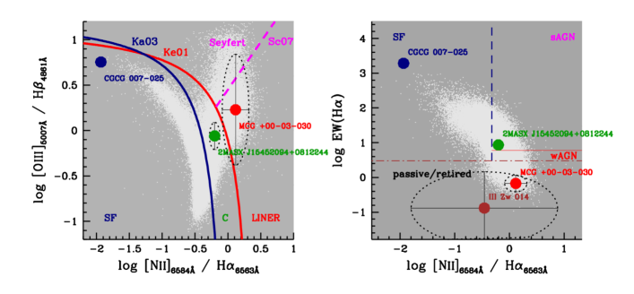
Figure 2: a) Loci of the three emission-line spectra (star-forming SF: CGC 007-025, composite (C): 2MASX J15452094+0812244 and LINER: MCG +00-03-030) fitted by fado (Figs. 3-5) on the BPT diagnostic diagram. The error bars and the ellipses depict 1$\sigma$ level uncertainties in the emission-line ratios. The demarcation lines correspond to the SF/Hii regime (blue; Kauffmann et al., 2003c) and AGN (red; Kewley et al., 2001). The division between Seyfert and LINERs is delineated by the magenta dashed line (Schawinski et al., 2007). b) WHAN diagram (Cid Fernandes et al., 2010, 2011) with the position of the four spectra fitted by fado in Sect. 7 are shown for the sake of comparison with the BPT classification. This alternative diagnostic diagram attempts to classifiy galaxies in SF, strong AGN (sAGN), weak AGN (wAGN) and passive/retired. In this diagram, we additionally include the tentative locus of the passive (lineless) galaxy III Zw 014, for which BPT emission-line ratios are unavailable. The white shaded area in both diagrams depicts the distribution of galaxies from SDSS.

Figure 3: a) Example of a spectral fit with fado of the star-forming region a in the low-metallicity BCD CGCG 007-025 (cf. e.g., Guseva et al., 2007). The SDSS spectrum of the source, corrected for Galactic extinction (orange curve), reveals intense nebular emission with a H$\alpha$ equivalent width of $\sim$2000 Å and strong contamination by nebular continuum emission, as apparent from the complete absence of stellar absorption features and the visible Paschen jump at 8207 Å. The best-fitting synthetic SED (open-blue) is composed of stellar and nebular continuum emission (dark gray and red, respectively). b) Residuals between fit and observed spectrum, with the shaded area and the dashed curve delineating, respectively, the $\pm$1$\sigma$ and $\pm$3$\sigma$ error spectrum. (c) Luminosity fraction at the normalization wavelength (6490 Å) and (d) stellar mass fraction of the SSPs composing the best-fitting population vector as a function of their age. The color-coding depicts the metallicity and the vertical bars $\pm$1$\sigma$ uncertainties. The thin-gray vertical lines connecting both diagrams correspond to the ages of the SSPs in the used library. The light-blue shaded area in both panels shows an Akima-smoothed (Akima, 1970) version of the SSP contributions, giving in panel d a schematic illustration of the star formation history. The electron temperature T_e and density n_e computed by fado from emission lines label the upper part of panel a, together with the probability $\pi$ of the spectrum to fall in the locus of SF, composite, LINER and Seyfert galaxies in BPT diagrams. Details on the meaning of the labels beneath the four panels are provided in the text. Panels c&d are shown without errors bars for the sake of better visibility.

Figure 3 shows a spectral fit to the SF region a of the nearby (D=21.6 Mpc) BCD CGCG 007-025 (cf. e.g., Guseva et al., 2007, hereafter G07). The presence of strong ongoing SF activity in this system is apparent from its SDSS spectrum (orange color in panel a), which shows a plethora of intense narrow nebular emission lines superimposed on a blue continuum with the Paschen discontinuity (8207 Å) visible in its red part. The best-fitting SED (open-blue) comprises stellar and nebular continuum emission (dark gray and red, respectively), with the latter contributing $\sim$50% of the monochromatic luminosity at $\sim$7400 Å and nearly 35% of the total luminosity of the modeled SED between 2750 Å and 9750 Å. Panel b shows the residuals between the observed and modeled spectrum, with the shaded area and the dashed lines delineating, respectively, the $\pm$1$\sigma$ and $\pm$3$\sigma$ error spectrum, as automatically determined by fado (cf. Sect. 2, $\alpha$4).

The spectral fit has been computed in the full-consistency mode (FCmode; Self-Con. 2) and assuming no LyC photon escape (Leakage: 0) with a library of 1326 SSPs from Bruzual & Charlot (2003) spanning a range in age between 1 Myr and 13.75 Gyr for six stellar metallicities (1/200, 1/50, 1/5, 1/2.5, 1 and 2.5 $Z_{\odot}$) for Padova 1994 evolutionary tracks (Alongi et al., 1993; Bressan et al., 1993; Fagotto et al., 1994a, b, c; Girardi et al., 1996), STELIB stellar library (Le Borgne et al., 2003) and the Chabrier (2003) IMF with a lower and upper mass cutoff of 0.1 and 100 M_⊙. That fado has reached convergence in the FCmode (2) can be read off the second number that follows the label Self-Con (lower-right), with the first one corresponding to the fitting mode initially chosen by the user (in this case 2, which is the default setting for SF/composite galaxies). The production rate of LyC photons capable of ionizing hydrogen (Q_H) and singly/doubly ionizing helium (Q_HeI, Q_HeII) that is predicted by the best-fitting PV is listed in the second column from bottom-left, and the third column gives a comparison between the observed and predicted (superscript obs and mod, respectively) H$\alpha$ and H$\beta$ fluxes (in $10^{-17}$ erg s^-1 cm^-2) and equivalent widths (in Å). It is worth noting that the predicted Balmer-line luminosities and nebular continuum are computed by taking into account the electron temperature and density (T_e=15205 K and n_e=171 cm^-3, respectively; cf. labels at the upper part of panel a) that have been derived from the observed spectrum in sub-module $\psi$2a. It can be seen that the model yields a good match to the observations, with regard to both the SED continuum (including the Paschen jump) and the H$\alpha$ and H$\beta$ flux and EW. We note that the [Oiii]-based electron temperature and EW(H$\beta$) inferred above are in reasonably good agreement with those from longslit spectroscopy by G07 (15.8 kK and 274 Å, respectively), which additionally reveals a strong Balmer jump shortwards of 3646 Å, in agreement with the SED predicted by fado.

The rightmost panels c&d display as a function of age the luminosity and mass contribution of individual SSPs in the best-fitting PV, with the color coding depicting their metallicity and the vertical bars 1$\sigma$ uncertainties. Gray vertical lines connecting the diagrams mark the ages of the SSPs in the used library (eventually, after AI-supported optimization through sub-module $\alpha$7 in case of a SSP base with more than 800 elements). The determined systemic velocity $v_{\rm sys}$ (in this and the following examples, $v_{\rm sys}$ is expressed relative to the recession velocity given by SDSS) and the intrinsic velocity dispersion ($\sigma_{\rm sys}$) are listed in the bottom-right column, along with the $V$-band extinction obtained for the stellar and nebular component (A_V and A${}_{\rm V\,neb}$, respectively) yielding a ratio of $\sim$1/2. This column additionally lists the determined log([Nii]/H$\alpha$) and log([Oiii]/H$\beta$) ratios, which place the galaxy on the BPT diagram (Fig. 2) in the locus of star-forming galaxies. The likelihood ($\pi$) in % for the spectrum being classifiable as SF, composite, LINER or Seyfert is given by the four numbers on the top-right of panel a (see Sect. 5 for details). Various other secondary quantities of interest are listed beneath the diagrams, such as the luminosity- and mass-weighted stellar age and metallicity, in both linear and logarithmic form (cf. Sect. 6), and the ever formed and presently available ${\cal M}_{\star}$, both the total one (M^e, M^p) and that of the post-AGB (age $\geq$ 100 Myr) stellar component (subscript pAGB). The vertical arrow in the log t vs M diagram (panel d) marks the age $t_{1/2}$ when 50% of the present-day ${\cal M}_{\star}$ has been in place.

The spectral fit in Fig. 3 illustrates several unique advantages of fado with special importance to studies of SF galaxies. One of them is its ability to converge even in the case of extreme nebular contamination, while reproducing key spectral features, such as the Paschen discontinuity and the hydrogen Balmer-line luminosities and EWs. This is not the case for spectral fits of SF galaxies with state-of-the-art (purely stellar) pss codes (e.g., STARLIGHT), for which an in-depth study by CGP17 reveals a strong (typically, one order of magnitude) discrepancy between the observed Balmer-line luminosities and those implied by the best-fitting stellar model. This discrepancy obviously also reflects the failure of these standard pss codes to place meaningful constraints on the recent SFH of galaxies, consequently also to other evolutionary indicators, such as the sSFR or recent-to-past SFR.

Spectral modeling with fado of low-metallicity, high-excitation BCDs, such as CGCG 007-025 can obviously benefit from inclusion of the Balmer jump, which future versions of the code will additionally take advantage of in order to supplement the model output with T_e determinations in the H⁺ zone (cf. e.g., Guseva et al., 2007) through an upgraded version of sub-module $\psi$2. In this context, it is also worth reiterating that already the nebular continuum in itself (i.e., the pure requirement posed in NCmode for the synthetic SED to reproduce the Balmer and Paschen jump, even without explicitly demanding the predicted hydrogen Balmer-line luminosities and EWs to match the observed ones) implicitly holds constraints that guide fado toward consistency between observed and predicted ne characteristics.

Figure 4: Spectral model with fado of the ”composite” galaxy (cf. Fig. 2) 2MASX J15452094+0812244. The meaning of the diagrams is identical to that in Fig. 3 except for panel b, which facilitates visual inspection of the quality of kinematical fitting of stellar absorption features within five selected spectral intervals. Additionally, we exclude from panels c&d the vertical bars estimated $\pm$1$\sigma$ uncertainties for the luminosity and mass contribution of individual SSPs, in order to facilitate visual inspection. It can be seen that emission lines in this system are weak (EW(H$\alpha$)$\leq$9 Å) and the nebular continuum is almost negligible throughout the considered spectral range.

Last but not least, an important feature of fado is that, despite a severely gas-contaminated spectral continuum, as in CGCG 007-025, it converges into a sensible stellar velocity dispersion $\sigma$ ($\approx$90 km/s) being within the range of values determined for dwarf galaxies (e.g., Guzmán et al., 1998) . This is not the case for conventional pss codes where strong dilution of stellar absorption features by the nebular continuum typically precludes computation of $\sigma$. This in turn may either prevent smooth termination of the fitting procedure or drive $\sigma$ to a maximum allowable bound, which could introduce a further bias in the inferred SFH. The so far poorly explored cumulative impact of the aforementioned limitations and biases stemming from the neglect of nebular continuum emission in currently available pss codes is certainly a subject of considerable relevance to studies of high-sSFR galaxies near and far (e.g., BCDs and green peas).

Figure 5: Spectral model with fado of MCG +00-03-030, an early-type galaxy that falls in the locus of LINERs (passive/retired) in the BPT (WHAN) diagram (Fig. 2). The layout is identical to that in Fig. 4 except for that in panel b, which here displays magnified versions of Gaussian line fitting and deblending of weak emission lines with an EW$<$1 Å.

We turn next to an example of fitting with fado of a spectrum classified as composite (Fig. 4). It can be seen that emission lines in this galaxy are weak, with the EW of the Balmer H$\alpha$ line being lower than 9 Å, and the EW(H$\beta$) comparable to the value expected for the underlying stellar absorption ($\sim$2 Å). Despite the weakness of the H$\alpha$ and H$\beta$ lines, fado could maintain the FCmode to full convergence (as apparent from the agreement between observed and predicted emission-line fluxes and EWs; third column from the left) and also indicated by the Self-Con label marking the initial and final fitting mode (2 in either case). However, since the auroral [Oiii]₄₃₆₃ emission line could not be detected in the observed spectrum, the electron temperature has been fixed to the standard value (T${}_{\rm e}=10^{4}$ K).

In Fig. 5, we show a spectral fit with fado of the early-type galaxy (ETG) MCG +00-03-030 that is classified (probability 0.44) as LINER, as is typically the case for such systems (see e.g., Gomes et al., 2016, and references therein). This fit also uses an extended library of 1326 SSPs from Bruzual & Charlot (2003). As apparent from comparison of panels a and b, emission lines in this galaxy are very weak (0.9 Å and 0.4 Å for the EW(H$\alpha$) and EW(H$\beta$), respectively) and visible only after subtraction of the best-fitting SED from the observed spectrum. The faintness of emission lines obviously precludes any accurate determination of T_e and n_e, which are therefore fixed to standard values ($10^{4}$ K and 100 cm^-3, respectively). For this reason, and because of the LINER nature of the source, fado switches from the initially attempted FCmode to the NCmode, with other words it drops the requirement for matching observed and predicted Balmer-line luminosities and EWs, while maintaining the contribution of nebular continuum in the SED fit.

Panel b is chosen to show for the sake of visual quality control a zoom-in into emission lines and their Gaussian fits. It can be appreciated that, even in the concrete case of a low-S/N, weak-line spectrum, the genetic DEO module of fado performs reasonably well in identifying and measuring emission lines. Given, however, the large uncertainties in the H$\alpha$ and H$\beta$ fluxes, the extinction in the nebular component is fixed to the value inferred for the stellar component. Note the strong discrepancy by a factor of $\tau\sim 60$ between predicted and observed Balmer-line fluxes, which, taken at face value, suggests that the bulk of the ionizing LyC radiation produced by the stellar component escapes without being locally reproduced into nebular emission (Papaderos et al., 2013; Gomes et al., 2016).

Finally, Fig. 6 shows a model to the lineless (”passive”, in the notation by Stasińska et al., 2008) galaxy III Zw 014. It can be seen that the quality of kinematical absorption-line fitting is satisfactory, with the exception of the Mg-feature, which reflects well-known imperfections of currently available SSPs in reproducing $\alpha$-enhancement features in ETGs (e.g., Worthey, Faber, & González, 1992; Worthey, 1992, 1994, see also Walcher et al. 2011 for a review).

Figure 6: Spectral model with fado of the lineless ”passive” galaxy (cf. Fig. 2) III Zw 014. The layout is as in Fig. 4.

8 Summary and conclusions

In this article, we outline the physical and mathematical concept, and present illustrative applications of fado (Fitting Analysis using Differential Evolution Optimization), a novel publicly available population spectral synthesis (pss) tool.

fado opens a promising avenue to the exploration of the assembly history of galaxies thanks to several unique features that go beyond existing concepts in spectral synthesis and which substantially alleviate degeneracies and systematic biases in state-of-the-art pss codes, all of which neglect nebular continuum emission and lack a mechanism that ensures consistency between the best-fitting star formation history (SFH) and the observed nebular emission characteristics. The main innovations embodied in fado pertain to both its astrophysical self-consistency concept and its mathematical realization:

i. Consistency between the best-fitting stellar model and the observed nebular emission characteristics in a galaxy: A key innovation of fado over all currently available pss codes is a) the inclusion of the nebular continuum emission in spectral fits. Nebular emission provides an important fraction (on the order of 1/3) of the total optical/IR continuum emission in galaxies undergoing strong star-forming activity, its consideration is therefore fundamental to a realistic and unbiased spectral modeling of such systems near and far; b) consistency between the observed nebular characteristics (luminosities and equivalent widths-EWs of hydrogen Balmer emission lines, shape of the continuum around the Balmer and Paschen jump) with the star formation- and chemical enrichment history inferred from the best-fitting stellar model.

ii. Multi-objective optimization to Pareto solutions with Differential Evolution Optimization: fado is the first pss code in astrophysics using an advanced variant of genetic Differential Evolution Optimization (DEO) algorithms. This and various other elements in its mathematical foundation and numerical realization (e.g., optimization of the spectral library used, test for convergence through a procedure inspired by Markov Chain Monte Carlo techniques) ensure quick convergence to the Pareto optimal solution. This, together with the stability, high computational efficiency (internal quasi-parallelization) and modular architecture of fado facilitates its non-supervized application to large spectroscopic data sets and eases future upgrades (e.g., integration of peripheral modules that permit a refined treatment of nebular physics and infrared emission by dust).

Quite importantly, fado incorporates within a single code the entire chain of data pre-processing, modeling, post-processing and graphical representation of the results from pss, including their storage in a convenient (FITS and postscript) format. This integrated concept greatly simplifies and accelerates a lengthy sequence of individual time-consuming steps generally involved in pssmodeling, this way further enhancing the overall efficiency of fado. Starting from the pre-processing of an input spectrum (flagging of emission lines and spurious spectral features and, optionally, flux-conserving rebinning, redshift determination and estimation of the error spectrum), fado uses Artificial Intelligence concepts for an initial spectroscopic classification and optimization of the library of Simple Stellar Population (SSP) spectra subsequently used for spectral fitting. Another unique feature of fado is the estimation of uncertainties for all primary quantities that define the best-fitting population vector, that is the mass and light contributions of individual SSPs involved in the fit, the intrinsic extinction (both for the stellar and nebular component) and the velocity dispersion. Uncertainties are computed and exported also for all secondary products from the model. These include a) various physical and evolutionary characteristics of a galaxy spectrum (e.g., luminosity- and mass-weighted stellar age and metallicity, ever formed and presently available stellar mass and the expected hydrogen- and helium-ionizing Lyman continuum photon rate from it, the time when a galaxy has assembled 1/2 of its present-day stellar mass, and others) and b) Fluxes and EWs, even for faint (EW$\la$1 Å) emission lines in the optical spectral range. Besides storage of the relevant primary and secondary output from spectral modeling (into FITS format) for subsequent analysis, fado also facilitates graphical visualization of its output (e.g., residuals between input spectrum and model, kinematics of the stellar component, emission-line fitting and deblending) through a built-in plotting routine.

Furthermore, fado incorporates already in its current publicly available version a number of additional features (currently under testing and fine-tuning) which will be offered in subsequent releases. These include the allowance for the estimation of the Lyman continuum photon escape fraction and the provision for a user-supplied instrumental line spread function for the sake of improved kinematical fitting and decomposition. Additionally, the presently unique ability of fado to handle spectral libraries with up to 2000 SSPs with a dimension of up to 24k each opens opportunities for the exploration with future higher-resolution SSPs of various topical questions in extragalactic research, such as, e.g., a possible non-universality of the stellar initial mass function or the $\alpha$-element enhancement in early-type galaxies.

Appendix A Illustrative comparisons of fado with state-of-the-art (purely stellar) population spectral synthesis codes

In this section we provide an illustrative comparison of results from fado and Starlight (Cid Fernandes et al., 2005, public distribution v04). The latter may be considered as representative of state-of-the-art pss codes, which without exception fit galaxy SEDs with purely stellar templates and lack a mechanism that ensures consistency between the observed nebular emission characteristics with the star-formation and chemical enrichment history encoded in best-fitting PVs (Sect. 1).

Figure 7: Spectral fit with fado to a synthetic spectrum from Rebetiko corresponding to an instantaneous-burst age of 3 Myr. The input spectrum includes nebular line and continuum emission computed from the LyC photon output from the stellar component, whereby case B recombination and standard conditions for the gas were assumed. The fit was computed in the FCmode of fado with the SSP library Base ${\cal F}$. The meaning of the panels is identical to that in Fig. 3.

Both pss codes were applied to synthetic spectra computed with our evolutionary synthesis code Rebetiko (Papaderos & Gomes, in prep.) for two SFHs, one involving continuous star formation at a constant SFR and the other a single instantaneous burst that is approximated by an exponentially decaying SFR $\propto\rm{exp}(-t/\tau)$ with a short e-folding timescale of $\tau=1$ Myr. For each SFH synthetic spectra were computed in the spectral range between 2500 – 10000 Å for 716 ages between 1 Myr and 15 Gyr, assuming solar metallicity ($Z_{\odot}=0.02$) and zero intrinsic extinction ($A_{V}=0$ mag). The SSP templates used by Rebetiko are from Bruzual & Charlot (2003), and assume a Chabrier (2003) IMF between 0.1 and 100 $M_{\odot}$ and Padova evolutionary tracks (Alongi et al. 1993; Bressan et al. 1993; Fagotto et al. 1994a, b, c; Girardi et al. 1996). For each synthetic SED, the LyC photon output from the stellar component (Zanstra, 1961) was converted into nebular continuum assuming case B recombination and standard conditions (T_e=10⁴ K, n_e=100 cm^-3; cf. Sect. 5). Additionally, Rebetiko exports into the synthetic SED hydrogen line fluxes computed for different electron temperatures and densities (Hummer & Storey, 1987), as well as lines for heavier elements adopted from the semi-empirical calibration by Anders & Fritze von Alvensleben (2003) as a function of the nebular metallicity. The synthetic stellar + nebular spectra from Rebetiko were finally smeared to an intrinsic velocity dispersion of 50 km/s both in the stellar and nebular component, and sightly degraded to a S/N=200 at $\lambda_{0}=4020$ Å.

In a second stage, the synthetic SEDs were modeled with Starlight and fado using a base that comprises SSPs from Bruzual & Charlot (2003) for 25 ages between 1 Myr and 18 Gyr and six metallicities ($Z=0.005$, 0.02, 0.2, 0.4, 1 and 2.5 $Z_{\odot}$), hereafter Base ${\cal S}$. Fits were performed after flagging of emission lines in the spectral range 3400 – 8900 Å following common practice in studies of local galaxy samples from SDSS (e.g., Asari et al., 2007; Ribeiro et al., 2016) with the $A_{V}$ kept as a free parameter between -1 and 4 mag. We note that, since fado allows a maximum of 2000 SSPs in the base library (Sect. 2.1), whereas the base in the case of Starlight is limited to 300 elements, a comparison between the two codes is only possible for SSP bases restricted to $\leq$300 elements.

Given that the computation of model uncertainties is not fully implemented in Starlight, each spectrum was fitted ten times with different initial guesses in the parameter space (seed numbers in the fitting procedure) to evaluate formal errors (see, e.g., Ribeiro et al., 2016; Cardoso, Gomes & Papaderos, 2016). Spectral fits with fado were computed in the FCmode and with the default number of evolutionary threads (7; cf. Sect. 3).

In the following, we restrict the comparison between the two pss codes to only a few physical quantities that one generally seeks to determine through pss modeling of galaxy spectra: the stellar mass ${\cal M}_{\star}$, light- and mass-weighted mean stellar age ($\langle\log t_{\star}\rangle_{{\cal L}}$ and $\langle\log t_{\star}\rangle_{{\cal M}}$, respectively), and light- and mass-weighted mean stellar metallicity ($\langle Z_{\star}\rangle_{{\cal L}}$ and $\langle Z_{\star}\rangle_{{\cal M}}$, respectively). Additionally, we compare the H$\alpha$ equivalent width of the input synthetic spectra with that implied by the best-fitting PV from fado as an additional means for evaluating the ability of the code to reproduce the nebular characteristics of a galaxy spectrum in its full-consistency fitting mode (FCmode). The reader is referred to CGP17 for detailed CPU-time benchmark tests of fado and a comparison of its output to that from currently available pss codes for synthetic galaxy spectra covering a wide range of SFHs, evolutionary stages and levels of nebular emission contribution. CGP17 also provide comparisons between the three fitting modes of fado (Sect. 5) for synthetic spectra of various characteristics (S/N ratio, wavelength coverage, spectral classification) and different model setups (e.g., number of evolutionary threads, dimension of the SSP library).

Figure 7 shows a fit with fado to a synthetic spectrum from Rebetiko for an instantaneous burst model of age 3 Myr. The figure layout is identical to that in Fig. 3. It can be seen that the best-fitting PV reproduces the Balmer and Paschen discontinuity (3646 and 8207 Å, respectively), and implies H$\alpha$ and H$\beta$ EWs (1682.9 and 262.7 Å, respectively) that closely match those of the input spectrum (1678.43 and 259.66 Å, respectively). Quite importantly, despite the strong nebular continuum contamination ($\sim$15 % of the monochromatic luminosity at $\sim$4020 Å) the mass- and luminosity-weighted age and metallicity of the stellar component are recovered by the model to within 5% difference.

Figure 8: Time evolution computed with Rebetiko of a) the Lick index H$\delta$_F, b) LyC photon rate per unit mass and c) H$\alpha$ emission-line equivalent width for an instantaneous burst (orange) and continuous star formation at constant SFR (red). The vertical blue strips on top of the panels mark the SSP ages for five stellar metallicities included in the fado-optimized library Base ${\cal F}$, which was compiled such as to simultaneously yield an adequate coverage of steep decline in the LyC photon rate in the first $\sim$40 Myr and the significant evolution of EWs of stellar absorption features (e.g., the H$\delta$_F Lick index) over the ensuing $\sim$1 Gyr in the evolution of an instantaneously formed stellar population. The SSP ages in Base ${\cal S}$ (green filled circles) are included for comparison.

Despite a long-standing controversy on inherent algebraic degeneracies in pss (e.g., Worthey, 1992; O’Connell, 1996; Pelat, 1997, 1998), a subtle yet important aspect in the periphery of this debate pertains to the construction of the SSP base. As we will argue below (and in more detail in CGP17), the commonly used small-to-medium size bases that generally comprise a limited number ($\la 200$ elements) of hand-picked SSPs is one of the causes for induced degeneracies in pss. This is because such bases are typically designed having in mind a reasonable trade-off between age/metallicity coverage and CPU-time expense. This task is in some cases aided by mathematical tools intended to eliminate nearly redundant elements in the SSP base and the grouping of base elements with similar properties into a single representative block using diffuse K-means algorithms Richards et al. (e.g., 2009). However, this approach is highly dependent on the number of cluster nodes spanning the base for spectral fitting. More importantly, a caveat of this approach is that depending on the number and selection criteria for cluster centers, short evolutionary phases that could hold decisive indicators that help constraining the fit (e.g., the steeply rising stellar H$\delta$ absorption-line EW in post-starburst galaxy spectra) might not be adequately covered by the base, which could then impact the best-fitting PV in a systematic or non-predictable manner, depending on the characteristics of the studied spectrum and the design of the SSP base. One simple example for this is that an attempt to fit a blue starburst-galaxy spectrum with a base lacking young SSPs might force the pss code to invoke a negative intrinsic extinction, just like in the case when a strongly subsolar (thus bluish) stellar component is modeled with solar/super-solar (thus reddish) SSPs. In other cases, however, for instance, when fitting of a post-starburst spectrum exhibiting strong ($\la$–6 Å) H$\delta$ stellar absorption features using a base that does not adequately cover ages between $\sim$0.1 and $\sim$0.7 Gyr, it is difficult to predict the resulting biases in the best-fitting PV. Another element to consider when aiming at consistency between the best-fitting PV and the observed nebular characteristics of a galaxy, as in the case of fado, is that instantaneously formed stellar populations (i.e., SSPs) show during early evolutionary stages (1–40 Myr) a relatively similar SED slope in the optical, but imply vastly different LyC photon rates, and in consequence of this, different hydrogen Balmer-line luminosities. A dense age (and metallicity) coverage for young SSPs is therefore essential for realizing and exploiting the self-consistency concept of fado in its FCmode and NCmode. A mathematically and astrophysically motivated construction of extended SSP bases that allows coverage in time and metallicity of phases associated with a strong evolution in the LyC photon production rate and the optical spectrophotometric characteristics of stellar populations is therefore crucially important. At the same time, large SSP libraries designed on the above criteria are well adapted to the capability of fado to cope with bases of up to 2000 elements.

From such considerations, we have selected SSPs to produce a fado-optimized base (Base ${\cal F}$) that densely traces the rapid decrease of the LyC output and the strong variation of the H$\delta$_F Lick absorption index in early ($\leq$40 Myr) and intermediate (0.1-1 Gyr) evolutionary stages (see Fig. 8). Ages of SSPs in Base ${\cal F}$ are depicted in the top of the figure, whereas filled green circles mark the ages composing the smaller SSP library Base ${\cal S}$. Base ${\cal F}$, containing 600 elements (100 ages between 1 Myr and 15 Gyr for six metallicities, $Z=0.005$, 0.02, 0.2, 0.4, 1 and 2.5 $Z_{\odot}$) was used for modeling with fado synthetic spectra computed with Rebetiko (e.g., Fig. 7).

Figure 9: Logarithmic representation of the difference between output and input stellar mass ${\cal M}_{\star}$ for spectral fits with fado and Starlight (blue and green, respectively) to synthetic spectra corresponding to a) a single-burst star formation scenario approximated by a declining SFR given by exp$(-t/\tau)$ with an e-folding timescale $\tau=1$ Myr and b) continuous star formation at constant SFR. The synthetic input spectra assume solar-metallicity and zero intrinsic extinction, and include the contribution of nebular emission (continuum and lines). The shaded green area around determinations with Starlight for the Base ${\cal S}$ SSP library depict $\pm$1$\sigma$ uncertainties, as obtained from ten fits. A substantial contribution of the reddish nebular continuum to the SED for ages lower than $\sim 10^{7}$ yr in panel a and lower than $\sim 10^{8}$ yr in panel b causes the purely stellar fits by Starlight to strongly overestimate ${\cal M}_{\star}$ by up to $\sim$1.8 dex. To the contrary, fado can recover ${\cal M}_{\star}$ to within less than $\sim$0.5 dex over the entire age interval considered. Results for spectral fits with Base ${\cal F}$are included in orange for the sake of completeness, but only for models with fado since this base contains 600 elements, twice the maximum number of base elements that Starlight can deal with. Note the significant improvement of the results from fado when Base ${\cal F}$ is used instead of Base ${\cal S}$, which is due to a better time coverage of evolutionary phases with a strong variation in the LyC photon rate and the H$\delta$_F absorption Lick index.

Figure 10: Difference between output and input of the mean stellar age $\langle\log t_{\star}\rangle_{{\cal M}}$ for synthetic spectra modeled with fado and Starlight. The colors have the same meaning as in Fig. 9.

Figure 9 shows as a function of evolutionary time the difference between the inferred and true ever formed ${\cal M}_{\star}$ for synthetic spectra modeled with fado and Starlight (green and blue, respectively). Spectral fits in either case were computed with the Base ${\cal S}$ library. The shaded green area around determinations from Starlight depict $\pm$1$\sigma$ uncertainties estimated from ten model runs. As a comparison, results from fado for the Base ${\cal F}$ library are overlaid in orange. The most salient feature from this diagram is that purely stellar fits with Starlight strongly overestimate ${\cal M}_{\star}$ by up to $\sim$1.8 dex for ages $\la 10^{7}$ and $\la 10^{8}$ yr for a single burst and constant SFR, respectively. This bias is apparent over the period in which the nebular contribution is significant (EW(H$\alpha$)$\gtrsim$100 Å; cf. Fig. 8).

Figure 11: Difference between output from fado for spectral fits with the Base ${\cal F}$ and input value of stellar mass ${\cal M}_{\star}$ (a), mean light- and mass-weighted stellar age (b&c), mean light- and mass-weighted stellar metallicity (d&e), and mean percentual deviation of the H$\alpha$ emission-line equivalent width (f). The synthetic input spectra were computed with Rebetiko assuming an instantaneous burst star formation scenario. In panel f the blue points correspond to equivalent-width of H$\alpha$ in emission below 0.5Å and the magenta points mark values in the range $0.5\AA\leq$ EW(H$\alpha$) $\leq 1\AA$. The green lines are three times the standard deviation over the whole age range of the models. The vertical blue strips on top of the diagrams depict the ages of the SSPs composing Base ${\cal F}$.

Figure 12: As in Fig. 11, but for synthetic spectra computed with Rebetiko assuming continuous star formation at a constant SFR.

This fact is also echoed by Fig. 10, where we show as a function of time the deviation of $\langle\log t_{\star}\rangle_{{\cal M}}$ from the true value for Starlight and fado fits. Starlight strongly overestimates the mean stellar age by up to 3.6 dex for ages $\la 10^{7}$ yr and $\la 10^{8}$ yr in the case of an instantaneous burst and constant SFR. We would like to point out that, for the latter SFH, purely stellar fits with Starlight result in a less prominent ($\la$0.8 dex) yet systematic overestimation of $\langle\log t_{\star}\rangle_{{\cal M}}$ for ages well beyond $>10^{9}$ yr. As for the results from fado, singular peaks due to degeneracies induced by the construction of the relatively small library Base ${\cal S}$ (see above) almost vanish when the fado-optimized SSP library Base ${\cal F}$ is used. The insights from both Fig. 9&10 underscore the conclusion by Izotov et al. (2011, see also Papaderos & Östlin 2012) that neglect of the reddish nebular continuum emission leads spectral fitting codes to infer a much too high fraction of old, high-M/L stars.

A more complete set of comparisons between fado (output) applied using the Base ${\cal F}$ library to synthetic spectra from Rebetiko (input) is shown in Fig. 11 & 12. These display for the same set of spectral models the difference between output and true stellar mass ever formed (a), light and mass-weighted stellar age (b&c), light and mass-weighted stellar metallicity (d&e). These figures additionally include the mean percentual deviation of the equivalent width of H$\alpha$ (f), in order to validate the full-consitency mode of fado. The uncertainties taking both set of models into account and using Base ${\cal F}$ are on average less than 0.05 dex and up to 0.15 dex for the stellar mass, on average less than 0.1 dex and up to 0.3 dex in the mean stellar age weighted both by light and mass. Light-weighted stellar metallicities are recovered within $\sim$0.15 dex and mass-weighted metallicities within $\sim$0.25 dex. In its FCmode, fado allows one to self-consistently reproduce the Balmer H$\alpha$ equivalent width within a mean percentual deviation of 10%. It is worth pointing out that the high mean percentual deviation of EW(H$\alpha$) in Fig. 11 for ages $7.5<$log(t)$<8.1$ is documented over an age interval where EW(H$\alpha$) has dropped to $<$0.1 Å, which means that it is negligible in absolute terms.