Stability of thin fluid films characterised by a complex form of structural/effective disjoining pressure

Abstract

We discuss instabilities of fluid films of nanoscale thickness, with a particular focus on films where the destabilising mechanism allows for linear instability, metastability, and absolute stability. Our study is motivated by nematic liquid crystal films; however we note that similar instability mechanisms, and forms of the effective disjoining pressure, appear in other contexts, such as the well-studied problem of polymeric films on two-layered substrates. The analysis is carried out within the framework of the long-wave approximation, which leads to a fourth order nonlinear partial different equation for the film thickness. Within the considered formulation, the nematic character of the film leads to an additional contribution to the disjoining pressure, changing its functional form. This effective disjoining pressure is characterised by the presence of a local maximum for non-vanishing film thickness. Such a form leads to complicated instability evolution that we study by analytical means, including application of marginal stability criteria, and by extensive numerical simulations that help us develop a better understanding of instability evolution in the nonlinear regime. This combination of analytical and computational techniques allows us to reach novel understanding of relevant instability mechanisms, and of their influence on transient and fully developed fluid film morphologies.

1 Introduction

Thin films, characterised by a small ratio of film thickness to typical lateral lengthscale, arise in many applications on scales that range from nano to macro. Recently, there has been much interest in instabilities of thin films on the nanoscale, in particular for polymeric films (see Seemann et al., 2001a; Sharma & Verma, 2004; Jacobs et al., 2008); nematic liquid crystal (NLC) films (see Herminghaus et al., 1998; Cazabat et al., 2011; van Effenterre & Valignat, 2003; Schlagowski et al., 2002; Ziherl et al., 2000); and metal films (see Favazza et al., 2007; Fowlkes et al., 2011), to name just a few examples. In many of the considered cases, the instabilities that develop are complicated by interplay of a number of different effects. On the nanoscale, these necessarily include fluid/solid interaction, often modelled by including in the governing equations a disjoining pressure term that plays an important role in determining the film stability. The relevant forms of the disjoining pressure may be rather complicated, reflecting, for example, complex Si/Si0₂ substrates in the case of polymer films (see Jacobs et al., 2008), or complex physics of the fluid/solid interaction in the case of metal films, see Ajaev & Willis (2003); Wu et al. (2010) and the references therein. Often, it is convenient to include additional physical effects to form a so-called “effective disjoining pressure”; these may include additional forces of electromagnetic origin, such as for ferrofluids in electric or magnetic fields (see Seric et al., 2014). For NLC films, such effective disjoining pressure is often called a structural disjoining pressure, since it includes the elastic forces that are due to the local structure of the director field (molecular orientation). Most work on this type of problem is carried out within the framework of long wave theory, which allows for simplifications of otherwise extremely complex free surface problems; we adopt this approach also.

In the context of NLC films, there are several experimental studies of dewetting on the nanoscale, e.g., Cazabat et al. (2011); van Effenterre & Valignat (2003); Schlagowski et al. (2002); Ziherl et al. (2000). For thin nematic liquid crystal (NLC) films deposited on SiO₂ wafer, the films were found to be unstable (dewetted) for a certain range of thicknesses, referred to as the “forbidden range” by Cazabat et al. (2011). Several different physical instability mechanisms have been proposed, and the discussion regarding the relevance of each is far from complete. Possibly relevant physical effects discussed in the literature include thermal effects (see Schlagowski et al., 2002; van Effenterre & Valignat, 2003) and the pseudo-Casimir effect (see Ziherl et al., 2000), as well as the interplay of elastic and disjoining pressure already discussed above (see Vandenbrouck et al., 1999).

The functional form of the (effective) disjoining pressure turns out to be similar for many of the setups discussed above; for example, for NLC films, the elastic effects lead to a disjoining pressure qualitatively similar to that found for polymer films on Si/SiO₂ substrates, or even for Newtonian films under inverted gravity conditions (hanging films); see Lin et al. (2013b); Lin & Kondic (2010). Our present work is motivated by NLC films, however as discussed above, the results are generally applicable for many other thin films with a similar form of effective disjoining pressure (see figure 1 later in the text).

Various instability mechanisms relevant to thin films have been discussed in the literature. For example, in addition to the standard linear stability analysis, which focuses on instabilities due to the presence of random infinitesimal perturbations (often called spinodal dewetting), there are instabilities due to the presence of nucleation centres (Seemann et al., 2001b; Sharma & Verma, 2004; Thiele et al., 2001; Diez & Kondic, 2007). Seemann et al. (2001b) further separate nucleation instabilities into two types: heterogeneous nucleation, characterised by nucleation holes with random (Poisson) distribution that emerge within a sharp time window; and homogeneous nucleation, possibly of thermal origin in experiments, where breakup is continuous and more and more nucleation holes form. In a similar direction, Thiele et al. (2001) and Diez & Kondic (2007) considered the metastable and absolutely stable regimes (stability of films with respect to perturbations of finite size). In this work, we explore these various stability regimes in the context of our NLC model and demonstrate parallels between stability properties of our model and the work of Seemann et al. (2001b); Sharma & Verma (2004); Thiele et al. (2001) and Diez & Kondic (2007), as well as similarities and differences between the referenced works.

The remainder of this paper is organised as follows. In § 2 we outline the derivation of the governing equation in the context of NLC films, highlighting differences between our model and others in the literature, especially with regard to the form of the effective (structural) disjoining pressure. In addition, appropriate scalings and physical parameters are discussed, and linear stability analysis (LSA) of a flat film is presented. The issues of particular relevance to NLC films are mostly considered in this section. We then proceed with a general discussion of film instability. In § 3 we discuss so-called spinodal instabilities, due to the presence of global (random) perturbations, intended to model the noise that is always present in physical experiments. Among other topics, we here discuss the formation of secondary (satellite) drops that are found only for a specific range of film thicknesses, and the distance between the emerging drops, whose dependence on the film thickness shows unexpected and rich structure. In § 4 we consider the influence of localised perturbations (nucleation centres) on the film stability. In this section we also apply the Marginal Stability Criterion to help us develop additional analytical insight regarding instability development; this approach (to the best of our knowledge) has not yet been discussed in the present context. We discuss both linearly stable and metastable regimes of instability. § 5 summarises our findings; of particular interest to the reader may be Fig. 19, which provides a summary of various instability mechanisms found and discussed throughout the paper.

2 Problem Formulation

We first outline our model for NLC films of thickness on the nano/micro scale, but emphasise that our results are of relevance to other types of thin films (such as polymeric films), which may be described by long-wave equations similar to ours (equation (10) later) and which involve an effective disjoining pressure qualitatively similar to that sketched in figure 1. For the thin films that we consider, the effects of gravity are negligible; however, van der Waals’ interactions, neglected in our previous work on thin film dynamics of NLCs (see Lam et al., 2015; Lin et al., 2013b), become important. Our model derives from the Leslie-Ericksen equations (Leslie, 1979), which comprise a fluid momentum equation plus incompressibility, analogous to Navier-Stokes; and an additional equation modelling conservation of energy (linear translational energy of the NLC molecules, and angular energy about each NLC molecule’s centre of mass). The fluid momentum equation differs from Navier-Stokes in two key ways: 1) by introducing a new anisotropic stress tensor (linear momentum), and 2) by an additional term modelling angular momentum. For brevity, the full derivation of the long wave model from the Leslie-Ericksen equations is skipped in the present paper; we present just a brief overview, highlighting where the modelling differs from our earlier work (Lin et al., 2013b).

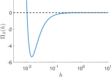
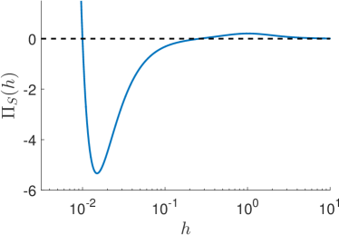
Figure 1: a) The disjoining pressure due to Van der Waals forces only (9) (${\mathcal{N}}=0$) and b) the total structural disjoining pressure, specified by (8); $h$ is the film thickness.

There are three crucial quantities in our long wave model: $h$, the free surface height; and the angles $\theta$, $\phi$ that characterise the director field, $\mathbf{n}$, a unit vector representing the local average orientation of the long axis of the rod-like NLC molecules. It is convenient to express the director field in polar coordinates, $\mathbf{n}=(\sin\theta\cos\phi,\sin\theta\sin\phi,\cos\theta)$, and consider the variables: $\theta$, the azimuthal angle; and $\phi$, the polar angle, which vary quasistatically via the film height $h$. Note that throughout this paper we use hats to distinguish between dimensional and dimensionless variables or parameters, hatted quantities being dimensional.

Analogous to Newtonian fluid models we include surface tension with constant surface energy density $\hat{\gamma}$, and van der Waals forces with volume energy density $\hat{A}$ (proportional to the Hamaker constant). Unique to NLCs (with respect to simple fluids) are the isotropic viscosity stress tensor, characterised by 6 coefficients, $\hat{\alpha}_{i}$ ($i=1,6$); and the elastic response, characterised by three constants $\hat{K}_{i}$ ($i=1,2,3$). Similar to other authors (Delabre et al., 2009; Rey, 2008; van Effenterre & Valignat, 2003; Ziherl & Z̆umer, 2003), we use the one-constant approximation, $\hat{K}=\hat{K}_{1}=\hat{K}_{2}=\hat{K}_{3}$. Furthermore, under the long wave approximation, only three of the six viscosities ($\hat{\alpha}_{3}$, $\hat{\alpha}_{4}$, and $\hat{\alpha}_{6}$) are relevant.

To nondimensonalise the Leslie-Ericksen equations five scaling factors are defined: $\hat{H}$, the film thickness; $\hat{L}$, the lengthscale of variations in the plane in the film, $(\hat{x},\hat{y})$; $\delta=\hat{H}/\hat{L}$, the small aspect ratio; $\hat{U}$, a characteristic flow velocity; $\hat{T}_{F}=\hat{L}/\hat{U}$, the timescale of fluid flow; and $\hat{\mu}=\hat{\alpha}_{4}/2$, a representative viscosity scale analogous to the Newtonian viscosity (with $\hat{\alpha}_{i}=0$ for $i\neq 4$, the isotropic viscosity stress tensor reduces to a simple Newtonian stress tensor). The choice of the scales is based on experimental data, and is further discussed in $\S$ 2.3.

2.1 Weak Free Surface Anchoring

In addition to the fluid flow timescale, $\hat{T}_{F}$, we may consider the timescale of elastic reorientation across the layer, $\hat{T}_{R}=\hat{\mu}\hat{H}^{2}/\hat{K}$. Assuming the timescale of reorientation is much faster than that of fluid flow, a quasistatic approximation (instantaneous elastic equilibrium) may be justified, and the energy equation may be solved to give the director field, $\mathbf{n}$, as a function of the instantaneous film height, $h$. In our previous work (see Lin et al., 2013b) we showed that the spherical director angles $\theta$ and $\phi$ are then given as

$$\theta=a(x,y,t)z+\theta_{S}(x,y,t)\quad\textrm{and}\quad\phi=\phi_{S}(x,y,t)\;,$$ (1)

where $a(x,y,t)$ depends on the free surface height, $h(x,y,t)$, as discussed below. The functions $\theta_{S}$ and $\phi_{S}$ depend on the preferred orientation of the NLC molecules at the interfaces, a phenomenon known as anchoring. We assume that the anchoring on the substrate is stronger than that at the free surface, and therefore that $\theta_{S}(x,y)$ and $\phi_{S}(x,y)$ are imposed by the substrate. In line with observations for physical systems, we assume $\theta_{S}$ is constant, while $\phi_{S}(x,y)$ may vary only spatially. This solution for the director feeds into the anisotropic stress tensor. The particular state here in which $\theta$ is linear in $z$ is often called the hybrid aligned nematic (HAN) state of NLCs.

In general, the preferred polar anchoring angles at the free surface, $\theta_{F}$, and at the substrate, $\theta_{S}$ (both assumed constant), are different (antagonistic anchoring). For very thin films, adjusting between these anchoring conditions incurs a large energy penalty in the bulk of the film. To reduce the energy penalty for very thin films, we allow the (weakly anchored) free surface director angle $\theta_{\mathcal{F}}$ to relax to the same value as the (strongly anchored) substrate director angle $\theta_{\mathcal{S}}$ for very thin films. Specifically, we take

$$\theta=\theta_{\mathcal{S}}+(\theta_{\mathcal{F}}-\theta_{\mathcal{S}})\frac{m(h)}{h}z\;,$$ (2)

$$m(h)=g(h)\frac{h^{2}}{h^{2}+\beta^{2}}\;,\quad g(h)=\frac{1}{2}\left[1+\tanh\left(\frac{h-2b}{w}\right)\right]\;,$$ (3)

where $m(h)$ is a relaxation function (directly related to the anchoring energy at the free surface, see Lin et al. (2013b)) in which $\beta$ is the thickness scale at which the bulk elastic energy is comparable to the free surface anchoring energy, and $g(h)$ is a ‘cut-off’ function (controlled by $w$) that enforces the substrate anchoring on the free surface when the film thickness is close to the equilibrium film thickness, $b$ (discussed in more detail later in the text).

Note that with this form of the director field, thicker NLC films are in the HAN state, while films close to the equilibrium thickness have a director field nearly homogeneous across the film thickness. This transition between the states is in agreement with several other models, e.g. Cazabat et al. (2011); Delabre et al. (2009); Ziherl et al. (2000). Furthermore, dimensional analysis shows that our lengthscale $\beta$ may be related to the extrapolation length discussed in the literature (Delabre et al., 2009; van Effenterre et al., 2001; Ziherl & Z̆umer, 2003).

2.2 Long Wave Model

To derive a long wave model for nanoscale thin films, we modify our earlier model, described in Lin et al. (2013b), by neglecting gravity and including van der Waals’ fluid-solid interaction. With this modification, there are five nondimensional parameters: ${\mathcal{C}}$, the inverse Capillary number, representing the ratio of surface tension and viscous forces; ${\mathcal{K}}$, the ratio of van der Waals’ and viscous forces; ${\mathcal{N}}$, a scaled inverse Ericksen number, representing the ratio of elastic and viscous forces; $\lambda$ and $\nu$, scaled effective viscosities. In terms of physical parameters,

$${\mathcal{C}}=\frac{\delta^{3}\hat{\gamma}}{\hat{\mu}\hat{U}}\;,\quad{\mathcal{K}}=\frac{\delta^{2}\hat{A}\hat{L}}{\hat{\mu}\hat{U}}\;,\quad{\mathcal{N}}=(\Delta\theta)^{2}\frac{\hat{K}}{\hat{\mu}\hat{U}\hat{L}}\;,\quad\Delta\theta=\theta_{\mathcal{F}}-\theta_{\mathcal{S}}\;,$$ (4)

$$\lambda=\frac{2+\eta}{4\left(1+\eta\right)}\;,\quad\nu=-\frac{\eta}{4\left(1+\eta\right)}\;,\quad\eta=\frac{\hat{\alpha}_{3}+\hat{\alpha}_{6}}{\hat{\mu}}\;,$$ (5)

where, recall, $\hat{\mu}=\hat{\alpha}_{4}/2$. For the remainder of the paper, only two-dimensional geometry will be considered; we leave the three-dimensional case for future work. The governing equation for the free surface height, $h(x,t)$, may then be expressed as

$$h_{t}+\left[\Phi\left({\mathcal{C}}h^{3}h_{xxx}+h^{3}{\Pi_{\textrm{S}}}^{\prime}(h)h_{x}\right)\right]_{x}=0\,,$$ (6)

$$\Phi=\left\{\begin{array}[]{rlr}\Phi_{\parallel}&=\lambda-\nu&\phi=0\\ \Phi_{\perp}&=\lambda+\nu&\phi=\frac{\pi}{2}\end{array}\right.\;.$$ (7)

Here $\Phi_{\parallel}$ denotes substrate polar anchoring parallel to the $x$-axis ($\phi=0$) and $\Phi_{\perp}$ denotes anchoring perpendicular to the $x$-axis ($\phi=\pi/2$); note that the value of $\Phi$ influences only only the timescale of fluid flow. Furthermore, if $\eta=0$, the governing equation (6) is independent of $\phi$ and our model corresponds to a fluid of isotropic viscosity. The structural disjoining pressure is defined as

$${\Pi_{\textrm{S}}}(h)={\mathcal{K}}f(h)+\frac{{\mathcal{N}}}{2}\left[\frac{m(h)}{h}\right]^{2}\;,$$ (8)

with $m(h)$ as defined in (3) above. Here, the second term on the right hand side is the response due to the antagonistic anchoring conditions, while the first term corresponds to the van der Waals’ disjoining pressure, taken here to be of power-law form

$$\Pi(h)={\mathcal{K}}f(h)={\mathcal{K}}\left[\left(\frac{b}{h}\right)^{3}-\left(\frac{b}{h}\right)^{2}\right]\;.$$ (9)

The form of the structural disjoining pressure, (8), is similar to that considered by Vandenbrouck et al. (1999); however, there are two important differences. First, the van der Waals term (9) considered here contains the repulsive term stabilising short wavelengths; this stabilisation is crucial if one wants to carry out simulations. Second, in the model of Vandenbrouck et al. (1999), the free surface azimuthal anchoring is assumed to be determined by the average initial thickness of the film and does not evolve with $h$. The power-law form of disjoining pressure (9) is used extensively in the literature; for a review see Craster & Matar (2009) and for further background regarding accounting for solid-fluid interactions, see Israelachvili (1992).

In the case (assumed henceforth) that $\phi$ is constant, a simple rescaling of time in (6) yields

$$h_{t}+\left[{\mathcal{C}}h^{3}h_{xxx}+h^{3}{\Pi_{\textrm{S}}}^{\prime}(h)h_{x}\right]_{x}=0\;,$$ (10)

with ${\Pi_{\textrm{S}}}$ as defined in (8). This equation will be considered in the rest of this paper. Note that in this model nematic effects enter only through modification of the disjoining pressure, by adding the structural component. Figure 1 shows typical forms of the disjoining pressure obtained using the parameter values discussed in the following. The structural disjoining pressure proposed in (8) is similar to that expected for many other film problems, in particular the well studied polymer films on Si/SiO₂ substrates, see, e.g. Seemann et al. (2001a). Therefore the results that we present in the rest of the manuscript are of relevance to a wide class of complex fluids.

Note: Equation (10) may be alternatively derived using the variational or gradient dynamics formulation (see Mitlin, 1993; Thiele et al., 2012). In this thermodynamically motivated approach the governing equation is expressed as

$$h_{t}+\nabla\cdot\left[Q(h)\nabla\left(\frac{\delta F}{\delta h}\right)\right]=0\;,$$ (11)

where $Q(h)$ is the mobility function, and $F$ is the free energy functional. Previous work (see Lin et al., 2013a) showed that, with consistent boundary conditions, the gradient dynamics formulation is equivalent to the long wave approximation of the Leslie-Ericksen equations. In terms of our model, $Q(h)=h^{3}$ and

$$F(h)=-{\mathcal{C}}\left[1+\frac{\left(\nabla h\right)^{2}}{2}\right]-\frac{{\mathcal{K}}b^{2}}{2h}\left[\frac{b}{h}-2\right]+{\mathcal{N}}\left[\frac{m(h)^{2}}{2h}-\int\frac{m(s)m^{\prime}(s)}{s}\;ds\right]\;.$$ (12)

2.3 Scalings and Physical Parameters

We now discuss the choice of scaling parameters mentioned in the beginning of $\S$ 2 and the material parameters in (4) and (5) for our model of thin NLC films (8) and (10). In experimental studies of dewetting of NLC films, the film thickness is typically of the order 10 to 100 nanometers (see Herminghaus et al., 1998; Vandenbrouck et al., 1999); therefore we set the representative film height $\hat{H}$ (used to scale $z$) to 100 nm. For temperatures far from a phase transition, the lower bound of the forbidden range of thickness is a few nanometers (it corresponds, in the experiments of Cazabat et al. (2011), to a trilayer of molecules). We define this lower bound to correspond to the equilibrium film thickness and set the equilibrium film thickness $\hat{b}=1$ nm. Bulk elastic energy is expected to be comparable to surface anchoring energy for film thicknesses in the 100 nanometers range; therefore we set $\hat{\beta}=100$ nm. Periodic undulations are observed on the free surface of films with a height on the order of $\hat{H}$, and in experiments by Cazabat et al. (2011) and Herminghaus et al. (1998), the wavelength of such undulations is observed to be in the range of 10-100 $\mu$m. Choosing the length scale in the $(x,y)$ domain $\hat{L}=10$ $\mu$m, we fix the aspect ratio $\delta=10^{-2}$. We choose the timescale of fluid flow $\hat{T}_{F}=\hat{L}/\hat{U}$ to match the timescale on which undulations develop in experiments, typically seconds to minutes (see Herminghaus et al., 1998); thus we set $\hat{T}_{F}=1$ s, corresponding to a velocity scale $\hat{U}=10$ $\mu$m s^-1.

The remaining parameters to be determined are: $\hat{\gamma}$, the surface tension; $\hat{K}$, the bulk elastic constant; $\theta_{F}$, free surface azimuthal anchoring angle; $\theta_{S}$, substrate azimuthal anchoring angle; $\hat{A}$, a force per unit volume, proportional to the Hamaker constant; and $\hat{\mu}$, a representative viscosity. Many experimental studies, such as Ausserré & Buraud (2011); Cazabat et al. (2011); van Effenterre & Valignat (2003); Poulard & Cazabat (2005); Schulz & Bahr (2011); Vandenbrouck et al. (1999) use the cyanobiphenyl (nCB) series of liquid crystals (where n refers to the number of carbons in the aliphatic tail), in particular, 4-Cyano-4’-pentylbiphenyl (5CB). Therefore, we choose these physical parameters to match 5CB data. It is noted by Cazabat et al. (2011) that, due to impurities in the NLC, published measurements of surface tension are scattered. However, to estimate the order of the non-dimensional parameters in our model, we note that surface tension appears typically to be of order $10^{-2}$ N m^-1, see Rey & Denn (2002); Cazabat et al. (2011). The elastic constant, $\hat{K}$, is of the order $10^{-11}-10^{-10}$ N (see Poulard & Cazabat, 2005; Delabre et al., 2008). For the nCB series of NLCs, the molecules prefer to align normal to the free surface (homeotropic anchoring) and in practice, substrates are often chosen and treated such that molecules align parallel to the substrate e.g. SiO₂; therefore we set $\theta_{F}=0$ and $\theta_{S}=\pi/2$. Accurate values for the characteristic viscosity of 5CB are difficult to find; however, Mechkov et al. (2009) was able to fit solutions of a thin film equation to experimental results (this work considers micron-scale drop thicknesses and the model used assumes strong free surface anchoring and neglects van der Waals interactions) with $\hat{\mu}$ of order $10^{-2}$ Pa s, a value in line with reported data (e.g. Inoue et al., 2002). Taking account of this available data, we choose $\hat{K}=1\times 10^{-11}$ N, $\hat{\gamma}=60\times 10^{-3}$ N m^-1, and $\hat{\mu}=60\times 10^{-3}$ Pa s.

In summary, the dimensional scaling factors are then fixed as

$$\hat{L}=10~{}\mu\textrm{m}\;,\;\;\hat{H}=100~{}\textrm{nm}\;,\;\;\hat{T}_{F}=1~{}\textrm{s}\;,\;\;\hat{T}_{R}=60~{}\mu\textrm{s}\;,\;\;\hat{U}=10~{}\mu\textrm{m~{}s\textsuperscript{-1}}\;.$$ (13)

Note that the assumption in $\S$ 2.1 that the timescale of elastic reorientation across the layer ($\hat{T}_{R}$) is much slower than that of fluid flow ($\hat{T}_{F}$) is satisfied. In addition, with the value of the contact angle to be discussed in $\S$ 2.3.1, the contact line velocity of a spreading NLC drop measured by Poulard & Cazabat (2005) (at the chosen contact angle) is of a similar order to our derived velocity scale $\hat{U}$.

Based on the scales discussed above, the dimensionless parameters we use (at least, for our initial investigations) are

$$\delta=0.01\;,\;\;{\mathcal{C}}=0.0857\;,\;\;{\mathcal{N}}=1.67\;,\;\;{\mathcal{K}}=0.0017\hat{A}~{}\textrm{m\textsuperscript{3}~{}J\textsuperscript{-1}}\;,\;b=0.01\;,\;\;\beta=1\;,$$ (14)

and $\hat{A}$, the volume energy density associated with van der Waals forces, is discussed next.

2.3.1 Contact Angle

To define a value for ${\mathcal{K}}$ (4), we relate the spreading parameter (a function of the contact angle) to the stored energy per unit area of the film using the Young-Laplace equation, see Diez & Kondic (2007). The spreading parameter $\hat{S}$ is given by

$$\hat{S}=\hat{\gamma}(1-\cos\theta_{c})=\hat{E}(\hat{h}=\infty)=-\int_{\hat{b}}^{\infty}\hat{\Pi}_{\textrm{S}}(\hat{h})\,d\hat{h}\;,$$ (15)

where $\theta_{c}$ is the equilibrium contact angle, $\hat{E}(\hat{h})$ is the stored energy per unit area, and $\hat{\Pi}_{\textrm{S}}(\hat{h})=(\hat{\mu}\hat{U}/\delta\hat{L})\Pi_{\textrm{S}}(h)$, where $\Pi_{\textrm{S}}$ is defined by (8): the usual van der Waals’ disjoining pressure plus the elastic “structural” component dependent on the function $m(h)$ and with prefactor ${\mathcal{N}}$. This elastic term of the integral in (15) can not be evaluated analytically, due to the complicated functional form of $m(h)$ as defined in (3). However, direct numerical integration shows (for the chosen values of $b$, $\beta$, and $w$), that the value of (15) is approximately the same if the approximation $g(h)=1$ in the definition of $m(h)$ is made (less than 1% difference). Setting $g(h)=1$, the integral in (15) may be evaluated analytically; but the result is not simple to work with. Therefore, we asymptotically expand in $\varepsilon=b/\beta=0.01\ll 1$ and keep the leading order term. The contact angles for NLC on Si (or SiO₂) substrates were measured by Poulard & Cazabat (2005) to be around $10^{-2}$ – $10^{-1}$ radians; thus assuming the contact angle is small, $\theta_{c}\ll 1$, (15) may be expressed as

$$\hat{A}=\frac{\hat{\gamma}\theta_{c}^{2}}{\hat{b}}\left(1+\kappa\left[\frac{\pi}{4}\varepsilon+O(\varepsilon^{4})\right]\right)\;,\quad\kappa=\frac{\hat{K}}{\hat{\gamma}\hat{b}\theta_{c}^{2}}\;.$$ (16)

To express (16) in terms of the nondimensional parameters (14), the order $\varepsilon^{4}$ term in (16) is neglected, and the approximated equation is multiplied by $\delta/\hat{\mu}\hat{U}$ to yield

$${\mathcal{K}}b\approx{\mathcal{C}}\left(\frac{\theta_{c}}{\delta}\right)^{2}+\frac{{\mathcal{N}}}{\beta\pi}\;,$$ (17)

where $b=\hat{b}/\hat{H}$ is the dimensionless equilibrium thickness. For the chosen values of $\hat{\gamma}$ and $\hat{K}$, and $\theta_{c}=0.06$, ${\kappa\pi\varepsilon/4}\approx 0.364$ in (16), therefore, it is reasonable to neglect the elastic contribution to the spreading parameter. This is in agreement with liquid crystals of low molar mass, where the anchoring energy on the free surface is usually significantly smaller than the isotropic surface tension energy, see Rey (2000). Neglecting the elastic term in (16) then, $\hat{A}=\hat{\gamma}\theta_{c}^{2}/\hat{b},$ and with $\theta_{c}=0.06$, we then obtain ${\mathcal{K}}=36.0$.

2.4 Linear Stability Analysis (LSA)

We now focus on the stability properties of a flat film, and in particular on the influence of the average film thickness, $H_{0}$. For this purpose, we first carry out LSA of a flat film solution to our governing equation (10). Assuming a solution of the form $h(x,t)=H_{0}+\epsilon e^{iqx+i\omega t}$ where $0<\epsilon\ll 1$, substitution in (10) yields the dispersion relation

$$\omega=iH_{0}^{3}\left[{\mathcal{C}}q^{2}-{\Pi_{\textrm{S}}}^{\prime}(H_{0})\right]q^{2}\;,$$ (18)

where

$${\Pi_{\textrm{S}}}^{\prime}(h)={\mathcal{K}}f^{\prime}(h)-{\mathcal{N}}\frac{M(h)}{h^{3}}\;;\quad M(h)=m^{2}(h)-hm(h)m^{\prime}(h);$$ (19)

with $f(h)$ defined by (9), $m(h)$ by (3) and parameters ${\mathcal{C}}$, ${\mathcal{K}}$, and ${\mathcal{N}}$ by (4); their values are given in § 2.3.

Assuming that $q$ is real, a film is always stable if ${\Pi_{\textrm{S}}}^{\prime}(H_{0})<0$, and is unstable otherwise. Therefore, the values of $H_{0}$ for which the film is unstable are the roots of

$$\frac{\Pi_{\rm S}^{\prime}(H_{0})}{\cal K}=f^{\prime}(H_{0})-\frac{{\mathcal{N}}}{{\mathcal{K}}}\frac{M(H_{0})}{H_{0}^{3}}\;,$$ (20)

which are calculated numerically and plotted (as two blue curves) in figure 2 in the $({\mathcal{N}}/{\mathcal{K}},H_{0})$-plane. In addition the roots of $f^{\prime}(H_{0})=0$ and $M(H_{0})=0$ are also plotted.

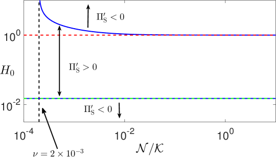
Figure 2: The zeros of (20) (blue curves), the zero of $M(H_{0})$ (dashed red line); and the zero of $f^{\prime}(H_{0})$ (dashed cyan line, lying almost entirely on the lower blue curve). The region enclosed by the blue curves denotes film thicknesses that are linearly unstable, i.e. ${\Pi_{\textrm{S}}}^{\prime}(H_{0})>0$. The dashed black line corresponds to a critical ${\mathcal{N}}/{\mathcal{K}}$ value; below that value, the destabilising van der Waals force is stronger than the stabilising elastic response.

Denoting the two roots of (20) as $H_{-}$ (the smaller root) and $H_{+}$ (the larger root), and noting that the region enclosed by blue curves corresponds to ${\Pi_{\textrm{S}}}^{\prime}(H_{0})>0$, figure 2 demonstrates that for $H_{0}\in(H_{-},H_{+})$, a flat film is unstable; therefore we conjecture that the unstable range of thicknesses in our model may be related to a range of so-called “forbidden thicknesses” noted experimentally by Cazabat et al. (2011). It can be seen that, for the range of ${\mathcal{N}}/{\mathcal{K}}$ considered, $H_{-}$ is closely approximated by the zero of the van der Waals term, i.e. $f^{\prime}(H_{-})\approx 0$; thus $H_{-}\approx 3b/2$ (see (9)): the lower thickness threshold between linear stability and instability is primarily determined by the van der Waals forces.

For ${\mathcal{N}}/{\mathcal{K}}>0.01$, the largest root of (20), $H_{+}$, corresponds approximately to the root of $M(H_{0})$, suggesting that for sufficiently strong elasticity, the upper threshold between linear instability and stability is determined by the antagonistic anchoring conditions (elastic response). For $H_{0}\gg b=0.01$, we may simplify $M(H_{0})$ (see its definition in (19)) by setting $g(H_{0})=1$ in (3), and $H_{+}\approx\beta$ can be found analytically. This is confirmed numerically using the values from $\S$2.3, which give ${\mathcal{N}}/{\mathcal{K}}=0.0514$; the second root of (20) is then found to be $H_{+}\approx 1.0150\approx\beta$ (see (14)).

In the linearly unstable regime, only perturbations with wavenumber $q\in(0,q_{c})$ are unstable; here $q_{c}$ is the critical wavenumber given by $q_{c}=\sqrt{{\Pi_{\textrm{S}}}^{\prime}(H_{0})/{\mathcal{C}}}$. The most unstable mode is given by $q_{m}=q_{c}\sqrt{2}=2\pi/\lambda_{m}$, with the growthrate

$$\omega_{m}={Q(H_{0})\left[{\Pi_{\textrm{S}}}^{\prime}(H_{0})\right]^{2}\over 4{\mathcal{C}}}={H_{0}^{3}\left[{\Pi_{\textrm{S}}}^{\prime}(H_{0})\right]^{2}\over 4{\mathcal{C}}}\,,$$ (21)

(see (11)). We will use these quantities later in the text. Note that in dimensionless form, $q_{c}$ and $q_{m}$ do not depend on the mobility function $Q(h)$ and the range(s) of unstable thicknesses is/are determined by ${\Pi_{\textrm{S}}}(h)$. Furthermore, the mobility function only affects the growth rate of the instability.

2.5 Comparison to other Models

There are several differences between the structural disjoining pressure used in our model (8) and others used in the literature. Unique to our model is weak free surface anchoring, which relaxes the free surface azimuthal anchoring as the film height evolves. This leads to a critical thickness value, $\beta$, below which the elastic contribution (ignoring van der Waals forces) is linearly destabilising for a flat film, and above which it is linearly stabilising. Furthermore, and as discussed above, figure 2 shows that for ${\mathcal{N}}\gg{\mathcal{K}}$, $H_{+}\approx\beta$, i.e. the upper bound between linear instability and stability is controlled by the elastic response. In comparison, the model presented by Vandenbrouck et al. (1999) sets the free surface azimuthal anchoring conditions to be a constant for all film thickness (the value of which is determined by the average initial film thickness). This is equivalent to strong anchoring ($m(h)=1$ in our model), which leads to the elastic response being always linearly stabilising; therefore, in the theory of Vandenbrouck et al. (1999), the upper threshold between linear instability and stability, $H_{+}$, is determined by the balancing of the destabilising van der Waals forces and the stabilising elastic response, regardless of the values of ${\mathcal{N}}$ and ${\mathcal{K}}$.

Furthermore, we note that the structural disjoining pressure term in our model may be expressed as

$$\begin{split}{\Pi_{\textrm{S}}}^{\prime}(h)h_{x}&={\mathcal{K}}f^{\prime}(h)h_{x}-\frac{{\mathcal{N}}}{h^{3}}\left[m^{2}(h)-hm(h)m^{\prime}(h)\right]h_{x}\\ &={\mathcal{K}}f^{\prime}(h)h_{x}-\frac{{\mathcal{N}}m^{2}(h)}{h^{3}}h_{x}-{\nabla{\mathcal{G}}(h)\over h}\;,\end{split}$$ (22)

where $\nabla{\mathcal{G}}(h)$ is the gradient of the free surface anchoring energy. The derivation of ${\mathcal{G}}(h)$ is nontrivial and we refer the reader to our previous work for further details (Lam et al., 2014; Lin et al., 2013b). Since the second term on the right hand side of the last equation in (22) is always stabilising, instability arises from the gradients of the free surface anchoring energy (the last term in (22)), present only for non-constant $m(h)$ (i.e., only for weak anchoring). Thus our model includes an alternative instability mechanism due to elastic forces not captured by the model in Vandenbrouck et al. (1999).

Excluding the $h^{-3}$ term from the van der Waals contribution to the disjoining pressure (9), the structural disjoining pressure in our model (8) is qualitatively similar to the total disjoining pressure derived by Ziherl et al. (2000). This term is, however, essential for the purpose of carrying out numerical simulations. In the work by Ziherl et al. (2000), the structural component to the disjoining pressure was derived by first considering the elastic energy due to fluctuations in the director field from some initial state. A critical thickness was defined such that, below this threshold, the initial director field state is uniform, and above, the director field is in the HAN state. Therefore our model has similar underlying physical mechanisms driving instability: 1) transition between a uniform director field for thin films to the HAN state for thick films; 2) interplay between bulk elastic energy and surface anchoring energy as the film thickness changes; and 3) inclusion of van der Waals forces.

However, there are also the following key differences: 1) the transition between the planar state and the HAN state is continuous in our model, whereas it is discontinuous in Ziherl et al. (2000); 2) Ziherl et al. (2000) assumed that the anchoring at the free surface was stronger than that at the substrate, therefore the uniform director field state for thin films was homeotropic in their model, while it is planar in ours; 3) to obtain similar linearly stable and unstable film thickness values with their model would require setting $\beta\approx 0.2$; and 4) only the total disjoining pressures are similar between the two models, the individual components (elastic contribution and van der Waals term minus the $h^{-3}$ term), are qualitatively different.

2.6 Numerical Scheme

In the following we will present a number of numerical simulations of our model in order to study its behaviour in detail. To solve the governing equation (10) numerically, we choose a spatial domain $x\in[0,x_{L}]$, and enforce periodic boundary conditions,

$$h_{x}(0,t)=h_{x}(x_{L},t)=h_{xxx}(0,t)=h_{xxx}(x_{L},t)=0\;,$$ (23)

where the right boundary $x_{L}$ will be fixed depending on the initial condition. The numerical method employed is a fully-implicit Crank-Nicolson type discretization scheme, with adaptive time stepping. A Newton iterative method is implemented at each time step to deal with nonlinear terms. More details about the numerical scheme can be found e.g. in Kondic (2003). For all numerical simulations shown in this paper, the grid size is fixed at the equilibrium film thickness, i.e. $\Delta x=b=0.01$ and, unless stated otherwise, the parameters in governing equation (10) are as given in § 2.3.

3 Films exposed to global perturbations

In this section, we present simulation results for films of thickness $H_{0}$ with superimposed perturbations that are global in character (cover the whole domain) and are intended to model infinitesimal random perturbations that are expected to be present in physical experiments. We focus on investigating film thicknesses in the linearly unstable regime, $H_{0}\in(H_{-},H_{+})\approx(0.015,1.015)$, and the morphology of dewetted films as a function of $H_{0}$. We start by discussing results for films perturbed by a single wavelength, on a domain equal in size to the imposed perturbation wavelength, and then proceed to consider random perturbations and large domains.

3.1 Simulations: Single Wavelength Perturbation

To begin, we validate the numerical scheme by comparing the growth rates extracted from numerical simulations to the expression (18) derived from LSA. The initial condition is of the form

$$h(x,t=0;H_{0},q)=H_{0}\left[1+0.01\cos(qx)\right]\;,\quad x\in[0,x_{L}]\;,\quad x_{L}=\frac{2\pi}{q}\;,$$ (24)

where $H_{0}$ and $q$ will be used to parameterise (24). In figure 3, the growthrates extracted from simulations are compared to those given by the dispersion relation. We see that the numerical simulations and LSA agree extremely well over the range of unstable film thicknesses and $q$ values considered.

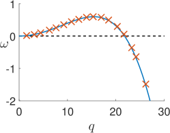
(a) $H_{0}=0.05$

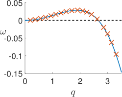
(b) $H_{0}=0.3$

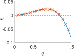
(c) $H_{0}=0.8$

Figure 3: Comparison of the dispersion relationship (solid blue curves) (18), and the growth rates extracted from numerical simulations ($\times$) for $H_{0}=0.05,\,0.3$ and $0.6$. Other parameters are given in $\S$2.3.

To proceed, we investigate in detail how the resulting film morphologies depend on the initial film thickness, $H_{0}$. Our simulations reveal that droplets may be classified according to their heights, with distinct droplet sizes emerging at different times over the course of a simulation. We therefore plot free surface height on a log scale in order to properly visualise smaller drops; also we show the free surface profile at four different times to illustrate the timescales on which dewetting and droplet formation occur.

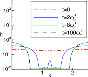
(a) $H_{0}=0.2$, $\omega_{m}^{-1}\approx 34.22$

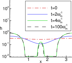
(b) $H_{0}=0.3$, $\omega_{m}^{-1}\approx 34.64$

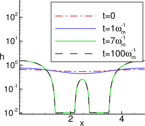
(c) $H_{0}=0.6$, $\omega_{m}^{-1}\approx 19.21$

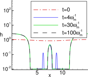
(d) $H_{0}=0.95$, $\omega_{m}^{-1}\approx 423.4$

Figure 4: Free surface evolution for various initial average film thicknesses, $H_{0}$. The initial condition is given by (24) with $x_{L}=\lambda_{m}$. Other parameters are given in $\S$2.3.

Figure 4, where $q=q_{m}$ (thus $x_{L}=\lambda_{m})$ in (24), shows the free surface evolution of the NLC film for several different values of the initial average film thickness, $H_{0}$. Initially, the perturbation grows, eventually forming large drops at the domain boundaries, as expected from LSA, and an additional secondary drop at the centre. On timescales much longer than the breakup time, comparable to $\omega_{m}^{-1}$, different dynamics emerge, however, depending on the film thickness $H_{0}$. For thinner films, shown in figure 4(a), the secondary drop persists for a short time only; while for thicker films, see figures 4(b) and 4(c), the secondary drops exist on a long time scale. For films near the critical thickness of linear instability, see figure 4(d), we observe an additional set of tertiary drops forming on either side of the secondary drop. These tertiary drops form at the same time as the primary drops, and exist on a timescale that is longer than that of dewetting, but shorter than that on which the secondary drop persists. We note that the times considered here are not asymptotically long, as considered by Glasner & Witelski (2003).

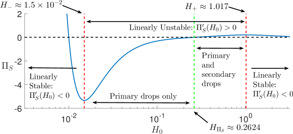
Figure 5: A summary of the final states obtained in simulations and their relationship to the structural disjoining pressure. The region enclosed by the dashed red lines is unstable. The dashed green line, at $H=H_{\Pi_{\textrm{S}}}$, corresponds to the zero of the structural disjoining pressure. These line patterns will be used consistently in all the following figures.

Figure 5 shows schematically our findings regarding film stability and existence of secondary drops on time scales that are long compared to $\omega_{m}^{-1}$. The region enclosed by the dashed red lines denotes the linearly unstable regime (determined by (19)), and the dashed green line corresponds to $H_{\Pi_{\textrm{S}}}\approx 0.2624$, the zero of the structural disjoining pressure ${\Pi_{\textrm{S}}}$ (8). The secondary drops are found only for film thicknesses with positive disjoining pressure, as we discuss further below in $\S$ 3.2. To the best of our knowledge, this finding is novel, and is one of the predictions of the present work. It would be of interest to verify it experimentally, not only for NLC films, but also for other films where positive disjoining pressures may be found, for example, for polymer films where positive disjoining pressure is due to fluid/substrate interaction; or for ferrofluid films in electric or magnetic fields (see Seric et al., 2014).

3.2 Simulations: Multiple Random Perturbations

To test the connection between the formation of secondary drops and the sign of the disjoining pressure, we carried out simulations in large domains with imposed perturbations of random amplitudes. The initial condition is defined as

$$h(x,t=0;H_{0},x_{L})=H_{0}\left[1+\epsilon\chi(x;x_{L})\right]\;,\quad\chi(x;x_{L})=\sum_{n=1}^{300}a_{n}\cos\left(\frac{nx}{x_{L}}\right)\;,\quad x\in[0,x_{L}]\;,$$ (25)

where $a_{n}\in[-1,1]$ are uniformly distributed, $\epsilon$ is chosen such that $|\epsilon\chi(x;x_{L})|\leq 0.01$ (i.e. the total perturbation size is bounded by $0.01$) , and $H_{0}$ and $x_{L}$ will be used to parameterise (25).

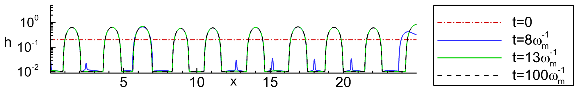
(a) $H_{0}=0.2$, $\omega_{m}^{-1}\approx 34.22$

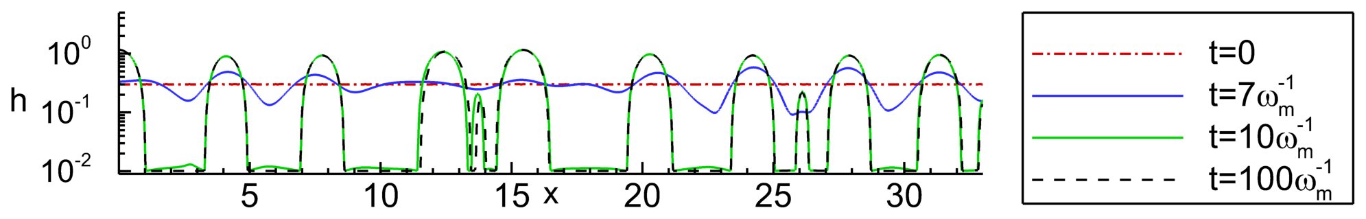
(b) $H_{0}=0.3$, $\omega_{m}^{-1}\approx 34.63$

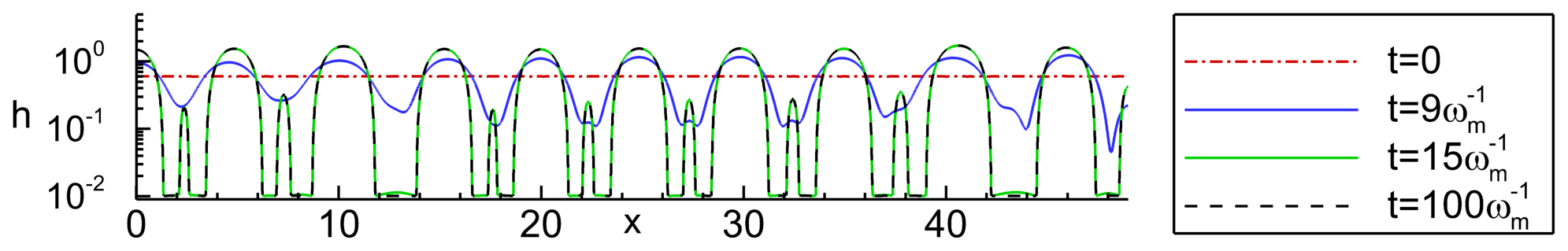
(c) $H_{0}=0.6$, $\omega_{m}^{-1}\approx 19.21$

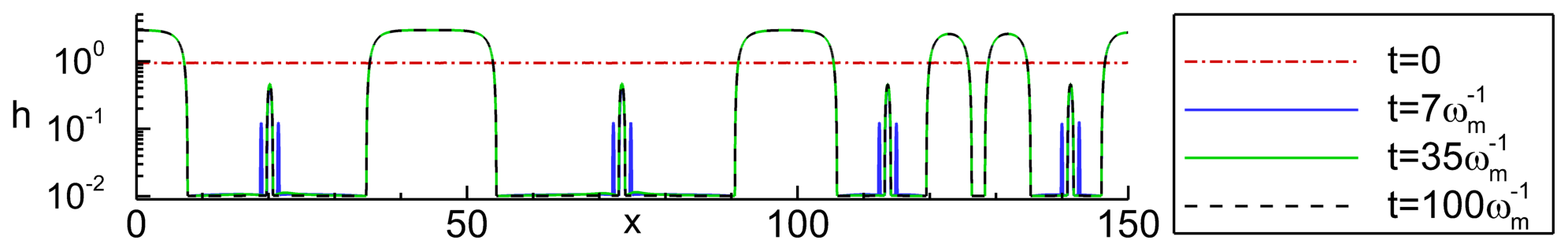
(d) $H_{0}=0.95$, $\omega_{m}^{-1}\approx 423.4$

Figure 6: Free surface evolution for various initial average film thicknesses, $H_{0}$. The initial condition is given by (25) with $x_{L}=10\lambda_{m}$. Other parameters are given in $\S$2.3.

Figure 6 shows the free surface evolution for initial condition (25) with $x_{L}=10\lambda_{m}$, and the same parameters and same range of initial thicknesses, $H_{0}$, as in figure 4. The main observation is that a minimum film thickness is still required for formation of long-lived secondary drops.

To discuss this finding in more detail, we also consider the drop sizes, defined by the heights of drop centres, $H_{l}$. Figure 7 shows a histogram of the log of the drop heights extracted from simulations corresponding to the same $H_{0}$ values as used in figure 6, but carried out on a larger domain ($x_{L}=50\lambda_{m}$) to improve statistics. We see that for $H_{0}<H_{\Pi_{\textrm{S}}}$, figure 7(a), the distribution is unimodal; and for $H_{0}>H_{\Pi_{\textrm{S}}}$, figures 7(b)-7(d), the distribution is bimodal (recall that $H_{\Pi_{\textrm{S}}}$ is the zero of the structural disjoining pressure, ${\Pi_{\textrm{S}}}(H_{\Pi_{\textrm{S}}})=0$). In addition, the dashed black line denotes the initial film thickness $H_{0}$, and it may be seen that $H_{0}$ provides an adequate threshold value between (larger) primary drops and (smaller) secondary drops (if they exist). The relevance of the dashed gold lines will be discussed shortly in $\S$ 3.3, but for now, note that as $H_{0}\rightarrow H_{+}$ (see figure 7(d)), the height of primary drops converges to the rightmost gold line.

To further illustrate the generality of our finding that secondary drops occur only if ${\Pi_{\textrm{S}}}(H_{0})>0$, we next consider the mode(s) of the drop heights, $\bar{H}_{l}$, the value(s) of which is/are given by the peak(s) of the distribution of $H_{l}$ in the histograms in figure 7, for two values of $\beta$ (the parameter defining the thickness where the bulk elastic energy is comparable to surface anchoring energy, see (8)). Figure 8 plots $\bar{H}_{l}$ as a function of $H_{0}$: the part (a) corresponds to the parameters used in figure 7 ($\beta=1$) and the part (b) shows the data for simulations with $\beta=2$. We clearly see that, in both cases, the secondary droplets appear only for film heights such that ${\Pi_{\textrm{S}}}(H_{0})>0$, and that $H_{0}$ (black dashed line) can be used to differentiate primary and secondary drops.

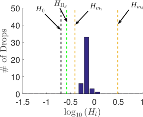
(a) $H_{0}=0.2$

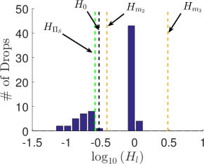
(b) $H_{0}=0.3$

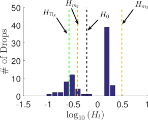
(c) $H_{0}=0.6$

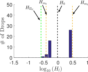
(d) $H_{0}=0.95$

Figure 7: Histogram of initial individual drop heights extracted from the corresponding simulations in figure 6. We see that when ${\Pi_{\textrm{S}}}(H_{0})>0$, panels (b), (c), and (d), the distribution is bimodal (primary and secondary drops), whereas for ${\Pi_{\textrm{S}}}(H_{0})<0$, panel (a), the distribution is unimodal (primary drops only). The black dashed line denotes the initial film thickness $H_{0}$ and dashed gold lines denote the range of metastable thicknesses, to be discussed in $\S$ 4.2.1.

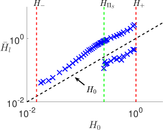
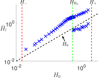
Figure 8: Mode(s) of drop heights (peak(s) of histogram data in figure 7) for (a) $\beta=1$, and (b) $\beta=2$. When ${\Pi_{\textrm{S}}}(H_{0})$ changes from negative to positive values (green dashed line), the distribution of the height of drop centres transitions from unimodal (primary drops only) to a bimodal distribution (primary and secondary drops). Furthermore, the initial film thickness, $H_{0}$ (black dashed line), proves an adequate threshold between the heights of the primary and secondary drops. Note that for $\beta=1,~{}2$, $H_{{\Pi_{\textrm{S}}}}=0.2624,~{}0.5275$, respectively.

3.3 Relation to Previous Work

Before closing this section we comment on the relation of our results to those previously reported in the literature on instabilities of polymer films. To begin, we extract the distances, $D_{l}$, between neighbouring primary drop centres (ignoring secondary drops with $H_{l}<H_{0}$), and normalise $D_{l}$ by $\lambda_{m}$. Figure 9 shows the mean distance, $\bar{D}_{l}$, for both the present model (figure 9) and for the Newtonian equivalent (figure 9). For $H_{0}$ not near the boundaries ($H_{\mp}$) of the linearly unstable regime (for Newtonian films, $H_{+}\rightarrow\infty$ within the present model that ignores gravity), $\bar{D}_{l}\approx 1.15\lambda_{m}$, consistent with LSA. Near the boundaries, however, $\bar{D}_{l}$ increases dramatically and is no longer related to $\lambda_{m}$. For very thin films (near $H_{-}$), the increase of $\bar{D}_{l}$ is due to coarsening occurring on a time scale similar to that of dewetting; therefore, drops merge before the entire film completely dewets. For thicker films (near $H_{+}$) the increase in the distance between drop centres appears to be due to a different mechanism that appears rather general, since it is operational for both NLC and Newtonian films. Note that for the same range of thicknesses, Seemann et al. (2001b) suggest that thermal (homogeneous) nucleation may be relevant; our results suggest that even without thermal effects (not included in our model), similar behaviour may emerge.

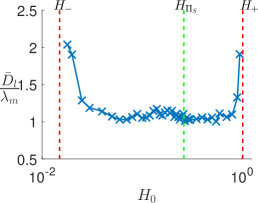
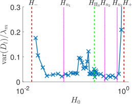
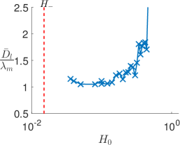
Figure 9: (a) Mean spacing between primary drop ($H_{l}>H_{0}$) centres, $\bar{D}_{l}$, normalised by $\lambda_{m}$; and (b) (variance in ${D}_{l})/\lambda_{m}$, for a randomly perturbed NLC film of thickness $H_{0}$. The dotted magenta lines denote thickness threshold values extracted from simulations of a film exposed to localised perturbations. The derivation and meaning of these lines will further discussed in $\S$ 4 and compared; for now, we note the increase in the variance in the region bounded by $H_{n_{1}}$ and $H_{n_{2}}$, and the region bounded by $H_{n_{1}}$ and $H^{+}$. (c) Distance between drop centres (no secondary drops) for a Newtonian film (${\mathcal{N}}=0$). Note that here there is no upper bound between linear instability and stability (i.e. $H^{+}$ is not defined) and all films thicker than $H_{-}$ (dashed red line) are unstable.

Regarding the formation of secondary drops, we note that previous works, such as Sharma & Verma (2004) or Thiele et al. (2001), do not report their existence. A possible reason for this may be the difference in scales. To see this, consider the ratio $\rho=H_{+}/H_{-}$. For the problem considered here, $\rho=O(10^{2})$, while in Thiele et al. (2001) and Sharma & Verma (2004), $\rho=O(1)$. Therefore, in the present problem it is possible to distinguish clearly features that may be invisible for smaller $\rho$.

Next, we discuss the shape of the primary drops. Figure 6 shows that for $H_{0}\rightarrow H_{+}$, the base of these drops widens. Such behaviour is found consistently for simulations with initial film thickness in the linearly unstable regime. In the example shown in figure 6(d), the primary drops at $x\approx 0,45,98,150$ are approximately flat for ten or more length units, then transition in height to the equilibrium film; therefore, ignoring the secondary drops, figure 7(d) may be interpreted as showing coexistence of two flat films, resembling NLC films observed on silicon (or silicon oxide) substrates, see Cazabat et al. (2011). Similarly to our results, as $H_{0}\rightarrow H^{+}$, Sharma & Verma (2004) observe the height profiles transitioning from “hills and valleys” (e.g. figure 6(c)) to “pancakes” (wide drops), see figure 6(d).

Sharma & Verma (2004) also show that an analytical result may be obtained for the minimum (equilibrium film thickness) and the maximum (height of drop centres) of steady state solutions. We will discuss an extension of these results to our setup later in $\S$ 4.2.1; for the present purposes it is sufficient to mention the prediction that, for sufficiently long times, the thickness value denoted by $H_{m_{3}}$ in figure 7 should be reached. We observe such behaviour only for $H_{0}\lessapprox H_{m_{3}}$ for the times considered. Once again, it is quite possible that the details of the influence of the film thickness could not be captured in Sharma & Verma (2004) due to insufficient separation of scales.

4 Films exposed to a Localised Perturbation

In this section we focus on instabilities induced by a localised perturbation, with the main motivation of comparing results with those of the preceding section obtained by global perturbations. Note that in physical experiments, such localised perturbations (also referred to as nucleation centres) may be a results of impurities, substrate defects, or some localised modification of the film structure.

We use the following initial condition

$$h(x,t=0)=H_{0}\left[1-d\exp\left(-\left[\frac{x}{0.2W}\right]^{2}\right)\right]\;,$$ (26)

i.e. a film of thickness $H_{0}$ with a localised perturbation at the left boundary, $x=0$, where a line of symmetry is assumed. The parameters $W$ and $d$ control the width and depth of the perturbation, respectively. We first present and discuss results for film heights in the linearly unstable regime, and then focus on the linearly stable regime in $\S$ 4.2.

4.1 Linearly Unstable Regime

Here we fix $d=0.1$ and $W=\lambda_{m}$ in (26). The domain length is initially set to $5\lambda_{m}$, and the right boundary is dynamically expanded as a simulation progresses. Our simulations should therefore be representative of a localised perturbation imposed on a film of infinite extent.

4.1.1 Computational Results

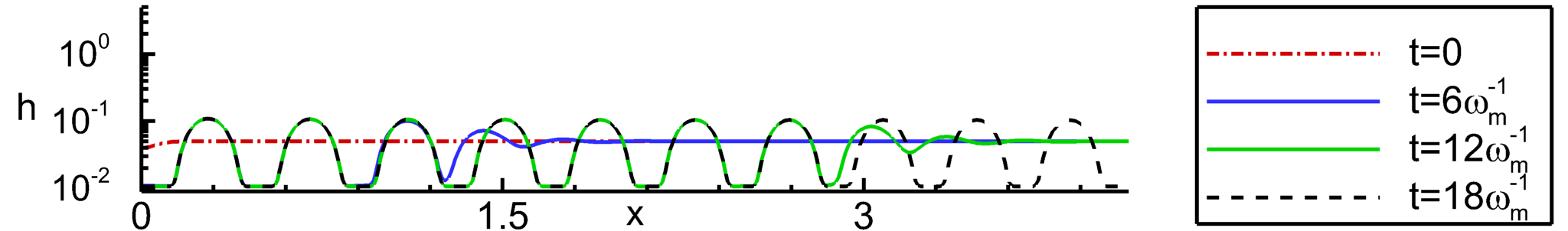
(a) $H_{0}=0.05$, $\omega_{m}^{-1}\approx 1.681$

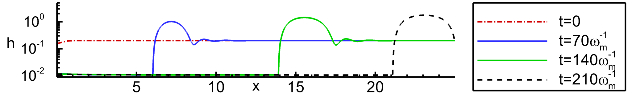
(b) $H_{0}=0.2$, $\omega_{m}^{-1}\approx 34.22$

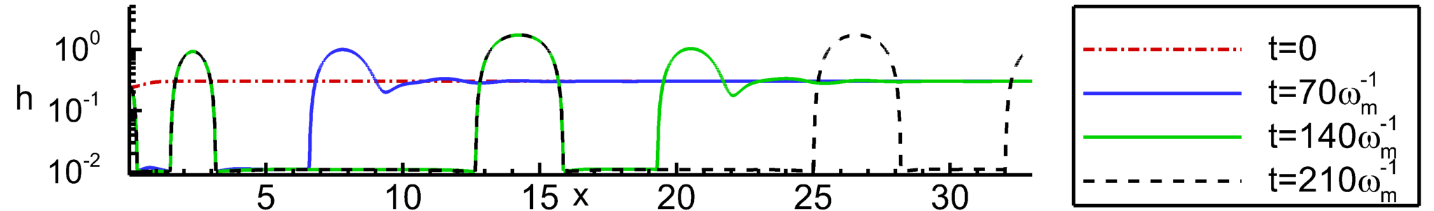
(c) $H_{0}=0.3$, $\omega_{m}^{-1}\approx 10.27$

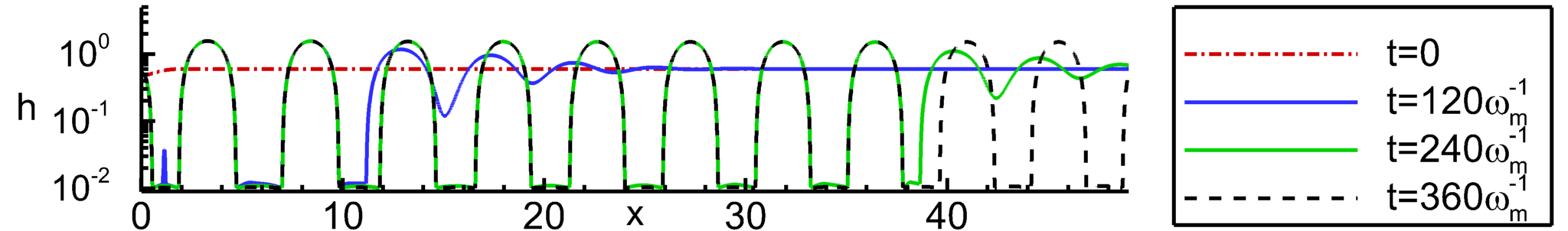
(d) $H_{0}=0.6$, $\omega_{m}^{-1}\approx 423.4$

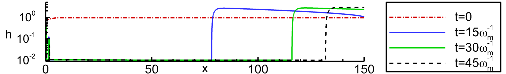
(e) $H_{0}=0.95$, $\omega_{m}^{-1}\approx 423.4$

Figure 10: The free surface evolution for various initial average film thicknesses, $H_{0}$. The initial condition is given by (26). Note that the film profiles shown in (b) and (e) form drops, but for times longer than shown here. The domain size shown in each panel is $10\lambda_{m}$; the simulation domains extend beyond the right boundary. The other parameters are given in $\S$2.3.

Figure 10 shows simulation results obtained with initial condition (26) and using the same parameter sets as in figures 4 and 6, as well as an additional thickness value, $H_{0}=0.05$. The main observation is that the localised perturbation propagates to the right and successively touches down forming drops; however, comparing the results of localised perturbation simulations to those obtained using random infinitesimal perturbations we note two main differences: first, no secondary drops are seen for localised perturbations; and second, the distance between drops is close to $\lambda_{m}$ only for some values of $H_{0}$; for example, in Fig. 10 the agreement with LSA is found only for $H_{0}=0.05$ and $H_{0}=0.6$, panels (b) and (d), respectively.

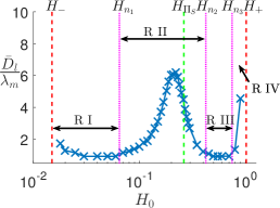
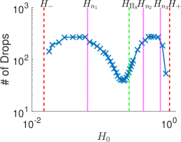
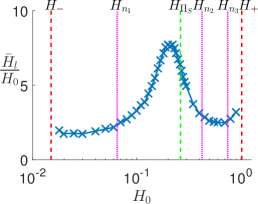
Figure 11: (a) The mean distance between drop centres, $\bar{D}_{l}$, normalised by $\lambda_{m}$, at $t=350\omega_{m}^{-1}$; (b) The corresponding number of drops; and (c) The mean height of drop centres, $\bar{H}_{l}$, normalised by $H_{0}$. The magenta dotted lines correspond to the values of $H_{0}$ for which $\bar{D}_{l}/\lambda_{m}$ crosses the value $1.1$. The other parameters are given in $\S$2.3.

To investigate further the dewetting process we calculate the mean distance between drop centres, $\bar{D}_{l}$. Figure 11 shows the results; to improve statistics, the simulations are carried out in large domains expanded in time to $320\lambda_{m}$. We observe the existence of four different regimes characterised by the magnitude of $\bar{D}_{l}/\lambda_{m}$, separated by three distinct film heights (marked by the dotted magenta lines showing where $\bar{D}_{l}/\lambda_{m}\approx 1.1$, to characterise departure from LSA predictions) and denoted $H_{n_{1}}$, $H_{n_{2}}$, and $H_{n_{3}}$. We see that in the regions marked R I and R III, the distance between drop centres is well approximated by $\lambda_{m}$; however, there exist regions R II and R IV, where there is no correlation between $\bar{D}_{l}$ and $\lambda_{m}$.

Regimes for which $\bar{D}_{l}\not\approx\lambda_{m}$ have been reported before (Thiele et al. (2001); Diez & Kondic (2007)) for different thin film models; however, the main findings differ from those presented here. In Thiele et al. (2001) and Diez & Kondic (2007) it is shown that there exists a $\bar{D}_{l}\not\approx\lambda_{m}$ regime near the upper threshold $H_{+}$ between linear instability and stability (see the R IV regime in figure 11). The work by Thiele et al. (2001) furthermore discusses a corresponding regime close to $H_{-}$; in the present formulation, this is a subset of the R I region very close to $H_{-}$ where, similarly to the results for a film exposed to random perturbations (see figure 9) the difference between $\bar{D}_{l}$ and $\lambda_{m}$ is due to coarsening occurring on the considered time scale. Neither of the previous works, however, discusses the existence of a (separate) R II regime.

Before exploring the instability development due to a local perturbation more rigorously, we first note a possible connection to our previous results for randomly perturbed films. Recalling the results for the mean distance between drop centres, $\bar{D}_{l}$, for films exposed to random perturbations (see figure 9), while $\bar{D}_{l}/\lambda_{m}\approx 1.15$ mostly everywhere, there appears to be small peak in $\bar{D}_{l}/\lambda_{m}$ in the thickness range corresponding to the R II regime. To highlight this connection further, in figure 9 the variance in $D_{l}/\lambda_{m}$ is plotted as a function of the initial film thickness $H_{0}$. We see that the variance increases in the R II and R IV regime, suggesting that there is a connection between the results for randomly and locally perturbed films. A possible explanation of this connection is that on large domains, the film does not dewet everywhere at the same time even if exposed to random perturbations; therefore, at the locations where the film dewets initially, the solution may appear as due to a localised perturbation, with retracting fronts modifying the distance between the drops that form eventually. The influence of these fronts may result in a large variance, explaining the results captured by figures 9 and 9.

We also note a possible connection to the theoretical and experimental results presented by Diez & Kondic (2007); Seemann et al. (2001b); and Thiele et al. (2001). Seemann et al. (2001b) suggest that as $H\rightarrow H_{+}$ (or $H_{-}$), where by definition ${\Pi_{\textrm{S}}}^{\prime}(H_{+})=0$ (${\Pi_{\textrm{S}}}^{\prime}(H)$ corresponds to $\phi^{\prime\prime}(h)$ in the referenced work), the barrier to nucleation vanishes, thus nucleation by thermal activation is possible. While our model does not include thermal effects, our results are similar to those observed by Seemann et al. (2001b). Therefore, the R IV regime in our results, and the nucleation reported by Diez & Kondic (2007) and Thiele et al. (2001) (again no thermal effects considered), may be analogous to the thermal nucleation regime.

Note: Under appropriate scaling, solutions of the form $h(x,t)=H_{0}[1+\epsilon h_{1}(x,t)+\epsilon^{2}h_{2}(x,t)+O(\epsilon^{3})]$, where $\epsilon\ll 1$, are to leading order independent of the model parameters. The scalings are as follows:

$$h=H_{0}\Psi\;,\quad x=\sqrt{\frac{{\mathcal{C}}}{{\Pi_{\textrm{S}}}^{\prime}(H_{0})}}\zeta\;,\quad\textrm{and}\quad t=\frac{{\mathcal{C}}}{Q(h)\left[{\Pi_{\textrm{S}}}^{\prime}(H_{0})\right]^{2}}\tau\;,$$ (27)

where for generality we keep the general mobility function, $Q(h)$. The rescaled leading order equation is

$$h_{1,\tau}+h_{1,\zeta\zeta\zeta\zeta}+h_{1,\zeta\zeta}=0,$$ (28)

and the mode of maximum growth and its corresponding growth rate are $\check{q}_{m}={1/\sqrt{2}},\;~{}\check{\omega}_{m}={1/4}$, respectively (here the check notation denotes the values obtained from the rescaled model). We see that as long as $h_{1}(x,t)=O(1)$ (i.e., as long as linear theory is applicable), the evolution for different choices of $H_{0}$ differs only by spatial and temporal scales. Recall that the initial conditions (24), (25), and (26) were chosen to scale with $\lambda_{m}$ and $H_{0}$, so the corresponding initial conditions in the rescaled variables are identical. The governing equation for $h_{2}(x,t)$ is

$$h_{2,\tau}+h_{2,\zeta\zeta\zeta\zeta}+h_{2,\zeta\zeta}=-\left[h_{1}\frac{Q^{\prime}(H_{0})}{Q(H_{0})}\left(h_{1,\zeta\zeta\zeta}+\left[1+\frac{Q(H_{0}){\Pi_{\textrm{S}}}^{\prime\prime}(H_{0})}{Q^{\prime}(H_{0}){\Pi_{\textrm{S}}}^{\prime}(H_{0})}\right]h_{1,\zeta}\right)\right]_{\zeta}\;,$$ (29)

for general $Q(h)$, and for $Q(h)=h^{n}$,

$$h_{2,\tau}+h_{2,\zeta\zeta\zeta\zeta}+h_{2,\zeta\zeta}=-\left[\frac{h_{1}}{H_{0}}\left(nh_{1,\zeta\zeta\zeta}+\left[n+\frac{H_{0}{\Pi_{\textrm{S}}}^{\prime\prime}(H_{0})}{{\Pi_{\textrm{S}}}^{\prime}(H_{0})}\right]h_{1,\zeta}\right)\right]_{\zeta}\;.$$ (30)

For any unstable film thickness $H_{0}$, the second order equations only differ by the forcing term on the right hand side, which is independent of the inverse Capillary number, ${\mathcal{C}}$, suggesting that the structural disjoining pressure determines the transition between different dewetting morphologies. Figure 12 plots the term enclosed by inner square brackets in (30) for $n=3$ and other parameters given in § 2.3. Note that this term is an increasing function of $H_{0}$ in the most of the R II regime (between $H_{n_{1}}$ and $H_{n_{2}}$), in contrast to its behaviour elsewhere. While we do not have clear explanation of the connection of this observation to the film breakup properties that we observe in the R II regime, we expect that it may be useful in future analysis of different stability regimes.

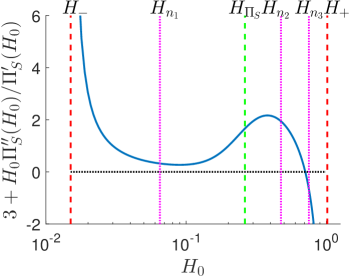
Figure 12: The inner square bracketed term in (29).

4.1.2 Marginal Stability Criterion: Outline

Marginal stability criterion (MSC) theory analyses front propagation into an unstable state using Fourier transforms and asymptotic theory. The analysis provides an expression for the velocity at which a front propagates into the unstable state asymptotically in time, and we will mainly focus our discussion on computing this velocity. In addition, the method specifies other possible wavelengths that may govern film breakup, and allows us to extract predictions for the expected time between the formation of successive drops (see Powers et al., 1998). To begin, we give a brief overview of MSC theory and its main results in the present context; the reader is referred to the comprehensive review by van Saarloos (2003) for further details. Then in the following section we discuss the correlation of MSC predictions with our computational results.

We assumed that the solution of the rescaled leading order governing equation (28) has a spatial Fourier series representation, i.e.

$$h_{1}(\zeta,\tau)=\int_{-\infty}^{\infty}\breve{h}_{1}(\check{q},\tau)e^{\check{q}\zeta i}\;d\check{q}\;.$$ (31)

Furthermore, with the ansatz

$$\breve{h}_{1}(\check{q},\tau)=\tilde{h}_{1}(\check{q})e^{-\check{\omega}(\check{q})\tau i}\;,$$ (32)

substituting (31) into (28) yields

$$\left[-i\check{\omega}(\check{q})+\check{q}^{4}-\check{q}^{2}\right]\int_{-\infty}^{\infty}\tilde{h}_{1}(\check{q})e^{\check{q}\zeta i-\check{\omega}(\check{q})\tau i}\;d\check{q}=0\;,$$ (33)

where $\tilde{h}_{1}(\check{q})$ is the Fourier transform of the initial condition, which is assumed to be an analytic function. Satisfying (28) for arbitrary $\tilde{h}_{1}(\check{q})$ gives the dispersion relation,

$$\check{\omega}(\check{q})=-i(\check{q}^{4}-\check{q}^{2})\;.$$ (34)

In the reference frame travelling with velocity $\check{V}$, the solution can be expressed as

$$h_{1}(s,\tau)=\int_{-\infty}^{\infty}\tilde{h}_{1}(\check{q})e^{i\check{q}s}e^{-i[\check{\omega}(\check{q})-\check{V}\check{q}]\tau}\;d\check{q}\;,$$ (35)

where $s=\zeta-\check{V}\tau$. If the above integral converges, $h_{1}(s,\tau)$ satisfies the rescaled governing equation (28), and $\check{V}$ is defined as the “linear spreading speed” by van Saarloos (2003).

Following van Saarloos (2003), we now consider the limit $\tau\rightarrow\infty$ and use a saddle-point approximation (steepest descent method) to approximate the integral in (35). The saddle-point $\check{q}^{*}$ satisfies

$$\check{V}=\left.\frac{d\check{\omega}(\check{q})}{d\check{q}}\right|_{\check{q}^{*}}\;.$$ (36)

To eliminate exponent terms of the integrand in (35) that lead to decay or growth in $\tau$, we set

$$\check{V}=\frac{\check{\omega}_{i}(\check{q})}{\check{q}_{i}}\;,$$ (37)

where $\check{V}\in\mathbb{R}$ (by definition), the $i$ subscript denotes the imaginary part of variables, and an $r$ subscript will be used to denote the real part. Recall $\check{\omega}(\check{q})$ is a polynomial in $\check{q}$ and thus differentiable, so that (36) may be expressed as

$$\check{V}=\textrm{Re}\left[\left.\frac{d\check{\omega}}{d\check{q}}\right|_{\check{q}^{*}}\right]=\left.\frac{1}{2}\left[\frac{\partial\check{\omega}_{r}}{\partial\check{q}_{r}}+\frac{\partial\check{\omega}_{i}}{\partial\check{q}_{i}}\right]\right|_{\check{q}^{*}}\;,$$ (38)

and

$$\textrm{Im}\left[\left.\frac{d\check{\omega}}{d\check{q}}\right|_{\check{q}^{*}}\right]=\left.\frac{1}{2}\left[\frac{\partial\check{\omega}_{i}}{\partial\check{q}_{r}}-\frac{\partial\check{\omega}_{r}}{\partial\check{q}_{i}}\right]\right|_{\check{q}^{*}}\;=0\;.$$ (39)

Furthermore, by definition, $\check{\omega}_{r}$ and $\check{\omega}_{i}$ satisfy the Cauchy-Riemann equations, simplifying (38) and (39) to

$$\check{V}(\check{q}^{*})=\left.\frac{\partial\check{\omega}_{r}}{\partial\check{q}_{r}}\right|_{\check{q}^{*}}\;,\quad\textrm{and}\quad\textrm{Im}\left[\left.\frac{d\check{\omega}}{d\check{q}}\right|_{\check{q}^{*}}\right]=\left.\frac{\partial\check{\omega}_{i}}{\partial\check{q}_{r}}\right|_{\check{q}^{*}}=0\;,$$ (40)

respectively. Satisfying the second condition in (40) gives an expression for $\check{q}_{r}$ as a function of $\check{q}_{i}$ and taking the derivative of (37) with respect to $\check{q}_{i}$ yields

$$\frac{d\check{V}}{d\check{q}_{i}}=\frac{1}{\check{q}_{i}}\left[\frac{\partial\check{\omega}_{r}}{\partial\check{q}_{r}}+\frac{d\check{q}_{i}}{d\check{q}_{r}}\frac{\partial\check{\omega}_{r}}{\partial\check{q}_{i}}-\frac{\check{\omega}_{i}(\check{q})}{\check{q}_{i}}\right]\;.$$ (41)

Evaluating the above equation at the saddle point, and substituting (37) and (40), we find

$$\left.\frac{d\check{V}}{d\check{q}_{i}}\right|_{\check{q}^{*}}=0\;,$$ (42)

and thus $\check{q}_{i}^{*}$ is a critical point of $\check{V}$. We note that this critical point is a minimum of $\check{V}$; however this information is not required to determine $\check{V}$ itself (see van Saarloos (2003) for further details). Equations (36), (40), and (42) provide the necessary conditions to determine $\check{q}_{r}^{*}$, $\check{q}_{i}^{*}$, and $\check{V}$. Therefore, with the rescaled dispersion relationship defined by (34),

$$\check{q}^{*}=\sqrt{\frac{3+\sqrt{7}}{4}}+\sqrt{\frac{1}{6}\left[\sqrt{7}-1\right]}i\approx 0.791+0.262i\;,$$ (43)

and

$$\check{V}=\frac{1}{9}\sqrt{1+\sqrt{7}}\left(5+\sqrt{7}\right)\approx 1.622\;\quad\textrm{and}\quad V\approx 1.622\frac{Q(H_{0})\left[{\Pi_{\textrm{S}}}^{\prime}(H_{0})\right]^{\frac{3}{2}}}{\sqrt{{\mathcal{C}}}}\;,$$ (44)

where the second equation in (44) is given in the unscaled variables. We note in passing that MSC also provides the condition for when a front propagating to the right will spread with the linear spreading speed asymptotically. If the initial condition decays faster than $e^{-\check{q}^{*}\zeta}$ as $\zeta\rightarrow\infty$, then the instability will spread with velocity $V$ given by (44), and the solution is referred to as a pulled front. For an initial condition that does not decay fast enough, the instability will propagate into the unstable state with a speed greater than $V$. The solution is then referred to as a pushed front and deriving an expression for the speed at which it spreads is nontrivial. For the present problem, the initial condition (26) is a Gaussian perturbation, thus decays sufficiently fast and a pulled front is expected.

Regarding the time scale for successive drop formation, we note that if a localised perturbation leads to a coherent pattern behind the front, it is periodic in time, i.e., $H(s)=H(\zeta-\check{V}\tau)=H(\zeta+\check{\lambda}-\check{V}\tau)=H(\zeta-\check{V}(\tau+\check{t}_{\textrm{MSC}}))$, where $\check{t}_{\textrm{MSC}}$ is the time between successive drops detaching from behind the front at distances $\check{\lambda}$ apart. Satisfying $H(\zeta+\check{\lambda}-\check{V}\tau)=H(\zeta-\check{V}(\tau+\check{t}_{\textrm{MSC}}))$ yields

$$\check{t}_{\textrm{MSC}}=\frac{\check{\lambda}}{\check{V}}=\frac{2\pi}{\check{q}\check{V}}\approx 5.478\;,\quad\textrm{or}\quad t_{\textrm{MSC}}=5.478\frac{{\mathcal{C}}}{Q(H_{0})\left[{\Pi_{\textrm{S}}}^{\prime}(H_{0})\right]^{2}}\;,$$ (45)

where, for future reference, $\check{q}=\check{q}_{m}$ was used in the first expression to obtain the second one. In the next section we proceed with correlating the presented MSC results with the computational ones.

Note 1: The speed of the propagating front, (44), may alternatively be obtained by using pinch point analysis, with a key difference of how the complex integral path is chosen in the Fourier representation (35). Our previous results (see Lam et al., 2014) for the flow of an NLC film down an inclined plane relied on the results of such analysis to derive the velocity of the wave packet boundaries ($V$ in the MSC analysis). In that work, analytical and numerical simulations confirmed the existence of three stability regimes behind the front travelling down the inclined plane: stable, convectively unstable, and absolutely unstable. These same instabilities were discussed by van Saarloos (2003) within a different physical context. The two unstable regimes were further subdivided into two cases: coherent pattern formation (periodic array of drops) and incoherent pattern formation; however, a general analytical theory for predicting these cases is not yet available. We will discuss our computational results within this context briefly in the next section.

Note 2: Having explicit results for the time scales on which localised and random perturbations lead to dewetting and drop formation, given by $t_{MSC}$ and $\omega_{m}^{-1}$, respectively, allows one to discuss which instability is relevant and actually destabilises a film. Considering the ratio of these time scales, however, shows it to be independent of the film thickness. This finding at first sight appears at odds with the commonly accepted paradigm that for thin films spinodal instability is relevant, while for thick ones nucleation is dominant, see, e.g. Seemann et al. (2001b). One explanation is that the nucleation instability may be operational for thin films as well (assuming that nucleating centres are available), but this is not obvious due to the same resulting wavelengths (for example, in the R II regime, see Fig. 11). However, more careful discussion of this important issue requires simulations in 3D, and we therefore defer it to future work.

4.1.3 Marginal Stability Criterion: Correlation with computational results

We now return to simulations of our model, and consider them in light of the MSC predictions. Using the analytical result (44) for the linear spreading speed, $V$, of the propagating perturbation, simulation results may be plotted in the reference frame moving with this speed. Furthermore, to emphasise the difference between the dewetting dynamics for different regimes, the travelling wave variable, $s=x-Vt$, is scaled by $\lambda_{m}$.

Figure 13 shows typical results in R II and R III regimes (the results in R I are similar to those in R III). First, we see that the instabilities caused by the localised perturbation are essentially bounded below $s=0$, demonstrating that MSC correctly predicts the speed with which instabilities propagate into the unstable flat region. Furthermore, since the front speed is given by MSC, we are in the pulled front case as expected. Second, the differences between the dewetting dynamics in various regimes are easily observed, and we discuss these differences next. Movies (Movie 1 - 4 in the online supplementary material) are also available to better illustrate the instability evolution.

In R III regime, see figure 13 and Movie 1, in the reference frame travelling with MSC speed $V$, the solution is a leftward-propagating travelling wave, with a stationary envelope (in the travelling reference frame). Furthermore, as the travelling wave propagates to the left, its amplitude (close to the front) grows monotonically and dewets the film periodically with wavelength $\lambda_{m}$, therefore leading to coherent pattern formation.

In R II regime, however, the instability evolution is more complicated. Here, the amplitude of the waves connecting the capillary ridge to the flat film (see e.g. $s/\lambda_{m}\in[-2,1]$ in figure  13) does not grow monotonically as it travels to the left, but oscillates until some critical amplitude is reached. In this regime (and similarly in R IV, not discussed for brevity), both coherent and incoherent pattern formation is possible; see Movies 2 -4 for examples that illustrate either coherent pattern formation (Movie 2); a bimodal pattern where drops of two different sizes are produced (Movie 3); or a disordered state, where the evolution resembles the R III regime sporadically interrupted by a different type of dynamics (Movie 4). Clearly, more work is needed to understand the details of pattern formation in R II (and R IV) regimes; we leave this for the future and for now focus on the main features of the results, without delving further into various modes of breakup in R II regime.

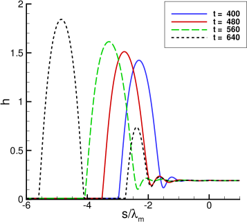
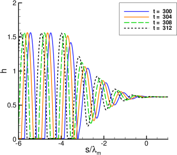
Figure 13: Typical evolution of the film thickness in the reference frame travelling with the linear spreading speed $V$ in (a) R II regime and (b) R III regime. Note that the $x$-axis has been scaled by $\lambda_{m}$ to highlight departure from the LSA predictions in R II regime.

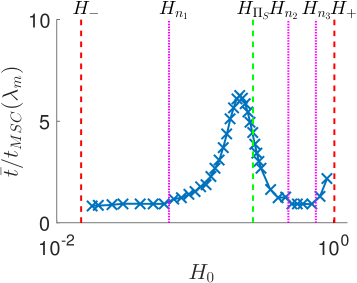
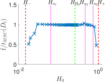
Figure 14: The mean time between drop formation extracted from simulations, normalised by (45) with (a) $\lambda=\lambda_{m}$ and (b) $\lambda=\bar{D}_{l}$, i.e. the mean distance between drop centres obtained in simulations.

To compare the film breakup times predicted by MSC (45) to the results of simulations, we extract the mean time between formation of successive drops. The results are plotted in figure 14 as a function of the initial film thickness, $H_{0}$, normalised by (45) with (a) $\lambda=\lambda_{m}$ and (b) $\lambda=\bar{D}_{l}$ (the mean distance between drop centres extracted from simulations). Similarly to the results given in figure 11, figure 14 shows that with $\lambda=\lambda_{m}$ the MSC prediction (45) gives good agreement with the numerics in regions R I and R III; however, there is no agreement in R II and R IV. Substituting instead the mean distance between drop centres $\lambda=\bar{D}_{l}$ into (45), figure 14 demonstrates that MSC gives the correct result for all film thicknesses not near the threshold values between instability and stability (dashed red lines). This result suggests that the MSC approach provides the correct result for breakup times once the instability wavelength is selected; however MSC does not provide information about this selected wavelength in the R II regime.

We note that, while a nonlinear variant of MSC has been developed, it applies only to pushed fronts (see van Saarloos, 2003) that are not relevant here. An alternative theory mentioned (but not thoroughly analysed) by van Saarloos (2003) is the Eckhaus or Benjamin-Feir resonance, based upon interaction between unstable waves. Further work is needed to analyse whether such interaction is responsible for the observed instability in R II and R IV regimes.

To summarise: for linearly unstable films subjected to a localised perturbation, we have extracted the mean spacing between drop centres and the mean formation times of successive drops, as a function of the initial film thickness, $H_{0}$. It has been shown that there exists a region, R II in figures 11 and 14, such that the results in the nonlinear evolution regime differ significantly from the predictions of LSA. Our understanding is that the effects leading to the existence of regimes R II and R IV are fully nonlinear.

4.2 Linearly Stable Regime

We now switch focus to locally perturbed films with initial film thicknesses in the linearly stable regime, in particular for $H_{0}>H_{+}$. First, we investigate the behaviour of linearly stable films exposed to a finite amplitude disturbance (metastability). Then, once dewetting is induced, we investigate the speed at which a localised perturbation propagates into the stable film region.

4.2.1 Metastability: Analytical findings

We first adapt the results of Thiele et al. (2001); Diez & Kondic (2007), and derive the metastable regime. Note that this regime is referred to as the heterogeneous nucleation regime by Seemann et al. (2001b); however, in contrast to the results to be presented here, Seemann et al. (2001b) provide no upper bound to this regime.

A linearly stable film is metastable if there exists a thinner, linearly stable, film with lower energy, hence, given a perturbation of sufficient size, the perturbation can push the thicker film into the energetically preferable thinner film state (dewetting). To derive an expression for the energy per unit length of a film, we analyse steady state solutions to the governing equation (10) that connect two flat films of different thicknesses.

To begin, we set $h_{t}(x,t)=0$ in (10), divide by $Q(h)=h^{3}$, and integrate with respect to $x$ to yield

$${\mathcal{C}}h_{xxx}+{\Pi_{\textrm{S}}}^{\prime}(h)h_{x}=d_{0}\;,$$ (46)

where $d_{0}$ is the constant of integration. Note that the metastability analysis from this point on is independent of the form of the mobility function $Q(h)$. Similarly to Sharma & Verma (2004), we use the far-field conditions

$$h(x\rightarrow-\infty,t)=H_{\textrm{min}}\;,\quad h(x\rightarrow\infty,t)=H_{\textrm{max}}\;,\quad H_{\textrm{min}}<H_{\textrm{max}}\;,$$ (47)

and

$$h_{x}(x,t)=h_{xx}(x,t)=h_{xxx}(x,t)=0\;,\quad x\rightarrow\pm\infty\;,$$ (48)

where $H_{\textrm{min}}$ and $H_{\textrm{max}}$ are constants to be determined. Applying boundary conditions (48) to (46), we find $d_{0}=0$. In the work of Sharma & Verma (2004), the solution that satisfies the above far-field conditions is referred to as a pancake solution. We will refer to this solution as a front solution since (47) and (48) are analogous to the far-field conditions used for a travelling front solution in our previous work (see Lam et al., 2014). Note that the same nomenclature is used by Thiele et al. (2001); the derivation of the front solution in that work is slightly different to that presented here, however, the two methods yield the same result.

Equation (46) is integrated in $x$ to obtain

$${\mathcal{C}}h_{xx}+{\Pi_{\textrm{S}}}(h)=\Pi_{0}\;,$$ (49)

where $\Pi_{0}$ is the constant of integration. To satisfy (47) and (48), we require ${\Pi_{\textrm{S}}}(h)$ to have the same value, $\Pi_{0}$, for at least two different thicknesses; i.e. ignoring the transition region between the flat films of thickness $H_{\textrm{min}}$ and $H_{\textrm{max}}$, the structural disjoining pressure is constant across the film. We may then parameterize steady state solutions, satisfying boundary conditions (47) and (48), by $\Pi_{0}$.

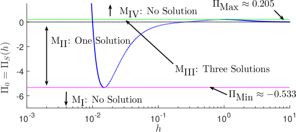
Figure 15: The solution space of (49) subject to conditions (47) and (48). Solid blue curves denote linearly stable films, and the dotted blue curve denotes linearly unstable ones.

Recalling figure 5, there are, at most, three different film thicknesses with the same disjoining pressure, hence there are at most three roots to ${\Pi_{\textrm{S}}}(h)=\Pi_{0}$, which we denote as $H_{m_{1}}$, $H_{m_{2}}$, and $H_{m_{3}}$, where $H_{m_{1}}<H_{m_{2}}<H_{m_{3}}$. Furthermore, we define four regimes: M_I (no roots), M_II (two roots), M_III (three roots), and M_IV (no roots), see figure 15. Note that $H_{m_{1}}$ and $H_{m_{3}}$ correspond to the left and right solid blue curves, respectively in Fig. 15 (thus represent linearly stable solutions), and $H_{m_{2}}$ is denoted by the central dotted blue curve (a linearly unstable solution).

In regions M_I and M_IV there are no possible solutions to the steady state boundary value problem specified by (47)–(49). Solutions exist for $\Pi_{0}\in(\Pi_{\textrm{Min}},\Pi_{\textrm{Max}})$, where $\Pi_{\textrm{Min}}$ and $\Pi_{\textrm{Max}}$ are the local minimum and local maximum of ${\Pi_{\textrm{S}}}(h)$ respectively, the values of which are given in figure 15 (for the chosen parameter values). In M_II, there are two roots of (47)–(49), thus one solution joining these states, with $H_{\textrm{Min}}=H_{m_{1}}$ and $H_{\textrm{Max}}=H_{m_{2}}$ i.e. the solution in M_II connects a thin linearly stable film to a thicker unstable one.

In M_III, there are three roots; thus we can choose two different $H_{\textrm{Min}}$ and $H_{\textrm{Max}}$, see figure 16. Since $H_{m_{2}}$ is a linearly unstable thickness, the corresponding steady state solutions are also unstable. Ignoring the unstable solution, we see that there is a one parameter family of stable steady solutions, which lies in M_III; thus we set

$$\Pi_{0}\in(0,\Pi_{\textrm{Max}})\;,\quad H_{\textrm{Min}}=H_{m_{1}}\;,\quad\textrm{and}\quad H_{\textrm{Max}}=H_{m_{3}}\;.$$ (50)

Integrating (49) with respect to $h$ yields (Euler–Lagrange equation)

$$\frac{{\mathcal{C}}}{2}\left(h_{x}\right)^{2}+e(h)=e_{0}\;,\quad e(h)=r(h)+\Pi_{0}h\;,$$ (51)

where $e(h)$ is the energy per unit length of the film due to the structural disjoining pressure. Here, the constant of integration $e_{0}$ may be interpreted as the total energy due to surface tension and structural disjoining pressure, and

$$r(h)=-\int{\Pi_{\textrm{S}}}(h)\;dh=\frac{{\mathcal{K}}b^{2}}{2h}\left[\frac{b}{h}-2\right]-{\mathcal{N}}\left[\frac{m^{2}(h)}{2h}-\int\frac{m(s)m^{\prime}(s)}{s}\,ds\right]\;.$$ (52)

Recalling the free energy functional (12), we note that $F(h)=-[{\mathcal{C}}(1+(h_{x})^{2}/2]-r(h)$. Setting $e_{0}=e(H_{m_{1}})$ we plot $e(h)-e_{0}$ in figure 16 for various $\Pi_{0}$, and observe that only for $\Pi_{0}>0$ are there two local minima for $e(h)-e(H_{m_{1}})$, see figure 16(b). In addition, we note that the film thicknesses at the local minima ($H_{m_{1}}$ and $H_{m_{3}}$) correspond to linearly stable films, and the film thickness at the local maximum ($H_{m_{2}}$) corresponds to a linearly unstable film.

Following Thiele et al. (2001), we seek a value of $\Pi_{0}$ such that the two local minima of (52) have the same energy. Specifically, we seek a value of $\Pi_{0}$ that satisfies

$$\frac{\partial e\left(H_{\textrm{min}}\right)}{\partial h}=\frac{\partial e\left(H_{\textrm{max}}\right)}{\partial h}=0\;,\quad$$ (53)

and

$$e\left(H_{\textrm{max}}\right)=e\left(H_{\textrm{min}}\right)\;.$$ (54)

Note that

$$\frac{\partial e}{\partial h}=0\,\,\Leftrightarrow\,\,{\Pi_{\textrm{S}}}(h)=\Pi_{0}\;,$$ (55)

therefore by inspection, (53) and (54) are equivalent to satisfying the far-field conditions, (47) and (48), in (49) and (51), respectively.

We now apply these results to the specific problem in question. For the parameters chosen in $\S$ 2.3, $\Pi_{0}=\Pi_{0}^{*}\approx 0.07273$ satisfies (53) and (54), and

$$H_{\textrm{Min}}^{*}=H_{m_{1}}^{*}\approx 0.99799\times 10^{-2}\;,\quad H_{m_{2}}^{*}\approx 0.39024\;,\quad H_{\textrm{Max}}^{*}=H_{m_{3}}^{*}\approx 3.05160\;,$$ (56)

where ‘*’ superscripts denote the values obtained by using $\Pi_{0}^{*}$ in Equation (49). The metastability regime is thus given by

$$H_{0}\in(H_{m_{1}}^{*},H_{-})\cup(H_{+},H_{m_{3}}^{*})\;.$$ (57)

The region $(H_{m_{1}}^{*},H_{-})$ corresponds to a narrow range of film thicknesses close to the equilibrium thickness, which we do not consider further. Films thicker than $H_{m_{3}}^{*}$ are absolutely stable, thus no perturbations may induce dewetting. The identified metastable region $(H_{+},H_{m_{3}}^{*})$ is considered by numerical simulations in the next section.

Note 1: In Seemann et al. (2001b), the metastable regime (heterogeneous nucleation in that work) is defined as $H_{0}>H_{+}$. Extending our presented metastability analysis to disjoining pressure models of Seemann et al. (2001b), we find that for all positive disjoining pressures values ($\Pi_{0}$ in (51)), condition (54) is never satisfied; specifically, we find that for all $\Pi_{0}>0$, $e\left(H_{\textrm{min}}\right)<e\left(H_{\textrm{max}}\right)$, hence there is no upper bound for the metastable regime, consistent with Seemann et al. (2001b). Therefore, the existence of absolutely stable films is one of the distinguishing features of the structural disjoining pressure considered here.

Note 2: Satisfying (53) implies that $H_{\textrm{Min}}$ and $H_{\textrm{Max}}$ are critical points of $e(h)$; however, to satisfy condition (53) with $H_{\textrm{Min}}\neq H_{\textrm{Max}}$, there must exist at least three distinct critical points, i.e., at least three different thicknesses must be characterised by the same disjoining pressure. In our model, this corresponds to positive disjoining pressure. This finding is in agreement with Herminghaus et al. (1998); Poulard et al. (2006); Seemann et al. (2001b), where it is stated that a disjoining pressure of the form shown in figure 1 will lead to metastability, a coexistence of films of different thicknesses.

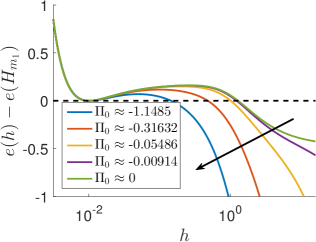
(a) $\Pi_{0}<0$

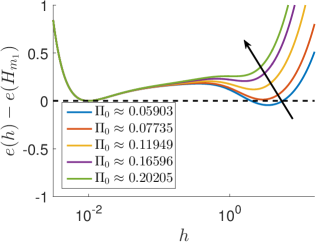
(b) $\Pi_{0}>0$

Figure 16: $e\big{(}h\big{)}-\big{(}H_{m_{1}}\big{)}$ where $e(h)$ is defined in (51) for an initial film profile with (a) negative structural disjoining pressure, $\Pi_{0}<0$; and (b) positive structural disjoining pressure, $\Pi_{0}>0$. Arrows denote the direction of increasing $\Pi_{0}$.

4.2.2 Metastability: Numerical Simulations

In this section, we investigate the evolution of localised perturbations in the metastable regime, $H_{0}\in(H_{+},H_{m_{3}}^{*})\approx(1.015,3.0516)$. The initial condition is specified by (26), which is parameterized by the initial film height, $H_{0}$. To explore the influence of the perturbation properties, we vary $W$ and $d$, respectively the width and depth of the perturbation. In particular, we discuss the quantity $d_{\textrm{Min}}(H_{0};W)$, the minimum perturbation amplitude required to induce dewetting. Since we are only interested if breakup occurs for a particular set of $d$ and $W$, it is not necessary to dynamically expand the right boundary in the $x$ domain; therefore, to reduce simulation time, we fix $x\in[0,200]$.

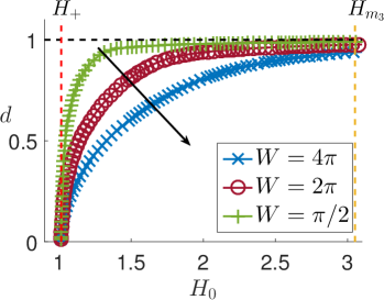
Figure 17: $d_{\textrm{Min}}(H_{0};W)$ as a function of $H_{0}$ for various values of $W$. Black arrow denotes direction of increasing $W$.

Figure 17 plots $d_{\textrm{Min}}(H_{0};W)$ as a function of $H_{0}$ for various values of $W$. In the region above $d_{\textrm{Min}}(H_{0};W)$ (curves with symbols) and below the dotted black line ($d=1$), the initial condition given by (26) induces dewetting. We see that for all values of $W$ considered, $d_{\textrm{Min}}(H_{0};W)\rightarrow 0$ as $H_{0}\rightarrow H_{+}$; i.e. as the film thickness approaches the threshold $H_{+}$ between linear stability and instability, an infinitesimally small perturbation ($d\ll 1$) will induce dewetting, as expected. More importantly, figure 17 demonstrates that as $H_{0}\rightarrow H_{m_{3}}$, $d_{\textrm{Min}}(H_{0};W)\rightarrow 1$; i.e. as the film thickness $H_{0}$ approaches the threshold $H_{m_{3}}$ between metastability and absolute stability, the initial condition (26) has to essentially rupture the film ($d\approx 1$) for dewetting to be observed. This demonstrates that the analysis in $\S$ 4.2.1 provides a correct upper bound for the metastable regime. Note that $d_{\textrm{Min}}(H_{m_{3}};W)$ is a monotonically decreasing function of the perturbation width $W$. This is expected, since the transition region between a film of thickness $H_{0}$ and the minimum of the initial condition (26) increases as $W$ increases, thus the transition region (which was assumed to be small and ignored in $\S$ 4.2.1) is no longer negligible.

Note 1: The presented results suggest that our model may transition between the regimes called thermal and heterogenous nucleation, see Seemann et al. (2001b). As $H_{0}\rightarrow H_{+}$ more and more holes are expected as the solution evolves, which may be a result of relatively small perturbations requiring more time to be experimentally measurable compared to the larger perturbations. In contrast, for $H_{0}$ significantly larger than $H_{+}$, only perturbations above the threshold value $d_{\textrm{Min}}$ will form holes, effectively enforcing an upper bound on the time window within which hole nucleation is observed. Therefore, as $H_{0}\rightarrow H_{+}$ from above, $d_{\textrm{Min}}\rightarrow 0$ and the time window ($\propto d^{-1}_{\textrm{Min}}$) in which holes form transitions from a sharp window, to a infinitely long time window, where more and more holes form in time.

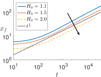
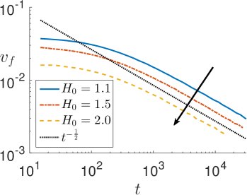
Figure 18: (a) Front position and (b) front speed as a function of time extracted for various initial film thicknesses, $H_{0}$, within the metastable regime. Black arrows denote direction of increasing $H_{0}$.

Note 2: We now briefly describe the film evolution once dewetting is induced. Similarly to simulations in $\S$ 4.1.1, the right boundary in the $x$ domain is dynamically expanded, and we set the initial domain to $[0,10]$. Simulations show that when dewetting occurs, a retracting front forms, and propagates without additional dewetting events into the flat film region. Similarly to Münch (2005), we extract from simulation results the time dependence of the front position, $x_{f}(t)$, and its speed, $v_{f}(t)$. Figure 18 shows that at long times scales, $x_{f}(t)\propto t^{1/2}$. Not surprisingly, this power law is different from the $t^{2/3}$, power law found by Münch (2005) for a thin film model in the slip dominated regime. Figure 18 shows that at long times scales, $v_{f}(t)\propto t^{-1/2}$, whereas in the linearly unstable regime, simulations and analysis show that propagation speed is a constant, see $\S$ 4.1.2.

5 Conclusions

While this work has been motivated by NLC films, we have presented results that are relevant to a much wider class of problems involving thin films on substrates, such that the fluid-solid interaction involves a relatively complex form of effective disjoining pressure (sketched on figure 19). Such a form has been derived in the present work as a structural disjoining pressure that includes an elastic contribution for NLC films; however similar functional forms have been extensively considered in the literature focusing on polymer films on Si/SiO₂ substrates, see, e.g. Jacobs et al. (2008) and the references therein.

In the NLC context, novel elements include dynamic relaxation of the free surface polar anchoring, $\theta_{F}$, as a function of film thickness $h(x,t)$. In addition, we have highlighted differences and similarities between the presented model, and others discussed in the literature, e.g. Cazabat et al. (2011); van Effenterre & Valignat (2003); Schlagowski et al. (2002); Ziherl et al. (2000). Furthermore, our model exhibits a range of film thickness such that a film is linearly unstable, which is analogous to the so-called “forbidden range” discussed in the literature (Cazabat et al., 2011).

More generally, an extensive statistical analysis of our computational results, combined with novel analytical results based on the Marginal Stability Criterion, has allowed us to identify a variety of instability mechanisms. In addition to the linearly unstable regime, where infinitesimally small perturbations induce dewetting, there are regimes that require perturbations of sufficient magnitude to induce dewetting (metastability), and regimes that are stable with respect to perturbations of any size (absolute stability). We have also identified the regimes that are linearly unstable, but susceptible to nucleation dominated dynamics. While we do not consider thermal effects, we find that for some film thicknesses (close to the stability boundaries) our results are similar to other results attributed to a thermal nucleation mechanism, suggesting that consideration of thermal effects may not in fact be needed to explain the dynamics. Also, we have formulated analytical procedures for identifying most of the stability regimes found computationally. In particular, the application of marginal stability analysis has allowed us to reach new insight.

Figure 19 summarises the various stability regimes uncovered, and correlates them with the form of structural/effective disjoining pressure. The following regions are identified:

1. [leftmargin=-.5in]

2. Linearly unstable regime, $H_{0}\in(H_{-},H_{+})\approx(1.5b,\beta)$, where $b$ is the equilibrium thickness and $\beta$ is the film thickness at which elastic force are relevant (see $\S$ 2.3 and $\S$ 2.4).

3. Linearly stable regime, $H_{0}\notin(H_{-},H_{+})$.

4. Linearly unstable regime with negative disjoining pressure, $H_{0}\in(H_{-},H_{\Pi_{\textrm{S}}})$, where $H_{\Pi_{\textrm{S}}}$ is the thickness marking the sign change of ${\Pi_{\textrm{S}}}$ (${\Pi_{\textrm{S}}}(H_{\Pi_{\textrm{S}}})=0$). If randomly perturbed, the film will dewet and form primary drops only (see $\S$ 3).

5. Linearly unstable regime with positive disjoining pressure, $H_{0}\in(H_{\Pi_{\textrm{S}}},H_{+})$. If randomly perturbed, the film will dewet and form primary and secondary drops.

6. Absolutely stable regime, $H_{0}<H^{*}_{m_{1}}$ or $H_{0}>H^{*}_{m_{3}}$. The film is stable with respect to any perturbation (see $\S$ 4.2).

7. Metastable regime, $H_{0}\in(H_{m_{1}}^{*},H_{-})\cup(H_{+},H_{m_{3}}^{*})$. A linearly stable film is unstable with respect to finite size perturbations.

8. Spinodal regime, $H_{0}\in(H_{-},H_{n_{1}})\cup(H_{n_{2}},H_{n_{3}})\subset(H_{-},~{}H_{+})$. A linearly unstable film perturbed by either localised or random perturbations will result in the mean distance between drop centres, $\bar{D}_{l}$, as predicted by LSA, i.e. $\bar{D}_{l}\approx\lambda_{m}$ (see $\S$ 4.1).

9. Nucleation regime within linearly unstable regime, $H_{0}\in(H_{n_{1}},H_{n_{2}})\cup(H_{n_{3}},H_{+})\subset(H_{-},~{}H_{+})$. A linearly unstable film perturbed by a localised perturbation will lead to $\bar{D}\not\approx\lambda_{m}$, and for a randomly perturbed film the variance in the distribution of inter-drop distances is significantly larger than for the spinodal regime, although we still find that $\bar{D}\approx\lambda_{m}$.

The regime often called ‘heterogenous nucleation’ includes the regimes (vi) and (viii); the ‘spinodal’ regime is defined under (vii).

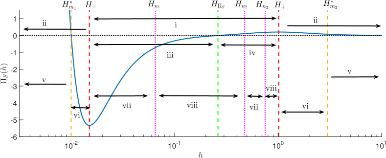
Figure 19: Summary of the various stability regimes discussed in this paper in relation to the structural/effective disjoining pressure. The dashed lines denote analytically derived values and dotted lines denote values extracted from numerical simulations. See the text for explanation of numbered regions.

There are several potential directions for future work. Statistical analysis has shown interesting connections between the observed phenomena and properties of the structural disjoining pressure; however, no clear physical mechanism has been identified analytically. Further investigation of the presented results is therefore required. Also, generalising our results to three dimensional flows is another area of interest, and is the subject of our ongoing research. We hope that our computational results, statistical analysis, and theoretical results will inspire future experimental and analytical investigations, which may provide additional insight into the phenomena presented.

Acknowledgements

The authors gratefully acknowledge financial support from NSF DMS 1211713 and CBET 1604351.

References

- Ajaev & Willis (2003) Ajaev, V. S. & Willis, D. A. 2003 Thermocapillary flow and rupture in films of molten metal on a substrate. Phys. Fluids 15, 3144.
- Ausserré & Buraud (2011) Ausserré, D. & Buraud, J.-L. 2011 Late stage spreading of stratified liquids: Theory. J. Chem. Phys. 134, 114706.
- Cazabat et al. (2011) Cazabat, A. M., Delabre, U., Richard, C. & Sang, Y. Yip Cheung 2011 Experimental study of hybrid nematic wetting films. Adv. Colloid Interface Sci. 168, 29.
- Craster & Matar (2009) Craster, R. V. & Matar, O. K. 2009 Dynamics and stability of thin liquid films. Rev. Mod. Phys. 81, 1131.
- Delabre et al. (2009) Delabre, U., Richard, C. & Cazabat, A. M. 2009 Thin nematic films on liquid substrates. J. Phys. Chem. B 113, 3647.
- Delabre et al. (2008) Delabre, U., Richard, C., Guéna, G., Meunier, J. & Cazabat, A. M. 2008 Nematic pancakes revisited. Langmuir 24, 3998.
- Diez & Kondic (2007) Diez, J.A. & Kondic, L. 2007 On the breakup of fluid films of finite and infinite extent. Phys. Fluids 19, 072107.
- van Effenterre et al. (2001) van Effenterre, D., Ober, R., Valignat, M. P. & Cazabat, A. M. 2001 Binary separation in very thin nematic films: Thickness and phase coexistence. Phys. Rev. Lett. 87, 125701.
- van Effenterre & Valignat (2003) van Effenterre, D. & Valignat, M. P. 2003 Stability of thin nematic films. Eur. Phys. J. E 12, 367.
- Favazza et al. (2007) Favazza, C., Trice, J., Kalyanaraman, R. & Sureshkumar, R. 2007 Self-organized metal nanostructures through laser-interference driven thermocapillary convection. Appl. Phys. Lett. 91, 043105.
- Fowlkes et al. (2011) Fowlkes, J. D., Kondic, L., Diez, J. & Rack, P. D. 2011 Self-assembly versus directed assembly of nanoparticles via pulsed laser induced dewetting of patterned metal films. Nano Letters 11, 2478.
- Glasner & Witelski (2003) Glasner, K. B. & Witelski, T. P. 2003 Coarsening dynamics of dewetting films. Phys. Rev. E 67, 016302.
- Herminghaus et al. (1998) Herminghaus, S., Jacobs, K., Mecke, K., Bischof, J., Fery, A., Ibn-Elhaj, M. & Schlagowski, S. 1998 Spinodal dewetting in liquid crystal and liquid metal films. Science 282, 916.
- Inoue et al. (2002) Inoue, M., Yoshino, K., Moritake, H. & Toda, K. 2002 Evaluation of nematic liquid-crystal director-orientation using shear horizontal wave propagation. J. Appl. Phys. 95, 2798.
- Israelachvili (1992) Israelachvili, Jacob N. 1992 Intermolecular and surface forces. New York: Academic Press, second edition.
- Jacobs et al. (2008) Jacobs, K., Seemann, R. & Herminghaus, S. 2008 Stability and dewetting of thin liquid films, p. 243. World Scientific, New Jersey.
- Kondic (2003) Kondic, L. 2003 Instability in the gravity driven flow of thin liquid films. SIAM Review 45, 95.
- Lam et al. (2014) Lam, M. A., Cummings, L. J., Lin, T.-S. & Kondic, L. 2014 Modeling flow of nematic liquid crystal down an incline. J Eng. Math. 94, 97.
- Lam et al. (2015) Lam, M. A., Cummings, L. J., Lin, T.-S. & Kondic, L. 2015 Three-dimensional coating flow of nematic liquid crystal on an inclined substrate. Eur. J. Appl. Maths 25, 647.
- Leslie (1979) Leslie, F. M. 1979 Theory of flow phenomena in liquid crystals. Adv. Liq. Cryst. 4, 1.
- Lin et al. (2013a) Lin, T.-S., Cummings, L. J., Archer, A. J., Kondic, L. & Thiele, U. 2013a Note on the hydrodynamic description of thin nematic films: strong anchoring model. Phys. Fluids 25, 082102.
- Lin & Kondic (2010) Lin, T.-S. & Kondic, L. 2010 Thin film flowing down inverted substrates: two dimensional flow. Phys. Fluids 22, 052105.
- Lin et al. (2013b) Lin, T.-S., Kondic, L., Thiele, U. & Cummings, L. J. 2013b Modeling spreading dynamics of liquid crystals in three spatial dimensions. J. Fluid Mech. 729, 214.
- Mechkov et al. (2009) Mechkov, S., Cazabat, A. M. & Oshanin, G. 2009 Post-Tanner spreading of nematic droplets. J. Phys.: Condens. Matter 21, 464134.
- Mitlin (1993) Mitlin, V. S. 1993 Dewetting of solid surface: analogy with spinodal decomposition. J. Colloid Interface Sci. 156, 491.
- Münch (2005) Münch, A. 2005 Detwetting rates of thin liquid films. J. Phys.: Condens. Matter 17, 309.
- Poulard & Cazabat (2005) Poulard, C. & Cazabat, A. M. 2005 Spontaneous spreading of nematic liquid crystals. Langmuir 21, 6270.
- Poulard et al. (2006) Poulard, C., Voué, M., De Coninck, J. & Cazabat, A. M. 2006 Spreading of nematic liquid crystals on hydrophobic substrates. Colloids and Surfaces A: Physicochem. Eng. Aspects 282, 240.
- Powers et al. (1998) Powers, T. R., Zhang, D., Goldstein, R. E. & Stone, H. A. 1998 Propagation of a topological transition: The Rayleigh instability. Phys. Fluids 10, 1052.
- Rey (2000) Rey, A. D. 2000 The Neumann and Young equations for nematic contact lines. Liq. Cryst. 27, 195.
- Rey (2008) Rey, A. D. 2008 Generalized Young-Laplace equation for nematic liquid crystal interfaces and its application to free-surface defects. Mol. Cryst. Liq. Cryst. 369, 63.
- Rey & Denn (2002) Rey, A. D. & Denn, M. M. 2002 Dynamical phenomena in liquid-crystalline materials. Annu. Rev. Fluid Mech. 34, 233.
- van Saarloos (2003) van Saarloos, W. 2003 Front propagation into unstable states. Phys. Reports 386, 29.
- Schlagowski et al. (2002) Schlagowski, S., Jacobs, K. & Herminghaus, S. 2002 Nucleation-induced undulative instability in thin films of nCB liquid crystals. Europhys. Lett. 57, 519.
- Schulz & Bahr (2011) Schulz, B & Bahr, C. 2011 Surface structure of ultrathin smectic films on silicon substrates: Pores and islands. Phys. Rev. E 83, 041710.
- Seemann et al. (2001a) Seemann, R., Herminghaus, S. & Jacobs, K. 2001a Dewetting patterns and molecular forces: a reconciliation. Phys. Rev. Lett. 86, 5534.
- Seemann et al. (2001b) Seemann, R., Herminghaus, S. & Jacobs, K. 2001b Gaining control of pattern formation of dewetting liquid films. J. Phys.: Condens. Matter 13, 4925.
- Seric et al. (2014) Seric, I, Afkhami, S. & L., Kondic 2014 Interfacial instability of thin ferrofluid films under a magnetic field. J. Fluid Mech. Rapids 755, R1.
- Sharma & Verma (2004) Sharma, A. & Verma, R. 2004 Pattern formation and dewetting in thin films of liquids showing complete macroscale wetting: From “pancakes” to “swiss cheese”. Langmuir 20, 10337.
- Thiele et al. (2012) Thiele, U., Archer, A. J. & Plapp, M. 2012 Thermodynamically consistent description of the hydrodynamics of free surfaces covered by insoluble surfactants of high concentration. Phys. Fluids 24, 102107.
- Thiele et al. (2001) Thiele, U., Velarde, M. G., Neuffer, K. & Pomeau, Y. 2001 Film rupture in the diffuse interface model coupled to hydrodynamics. Phys. Rev. E 64, 031602.
- Vandenbrouck et al. (1999) Vandenbrouck, F., Valignat, M. P. & Cazabat, A. M. 1999 Thin nematic films: Metastability and spinodal dewetting. Phys. Rev. Lett. 82, 2693.
- Wu et al. (2010) Wu, Y., Fowlkes, J.D., Rack, P. D., Diez, J.A. & Kondic, L. 2010 On the Breakup of Patterned Nanoscale Copper Rings into Droplets via Pulsed-Laser-Induced Dewetting: Competing Liquid-Phase Instability and Transport Mechanisms. Langmuir 26, 11972.
- Ziherl et al. (2000) Ziherl, P., Podgornik, R. & Z̆umer, S. 2000 Pseudo-casimir structural force drives spinodal dewetting in nematic liquid crystals. Phys. Rev. Lett. 84, 1228.
- Ziherl & Z̆umer (2003) Ziherl, P. & Z̆umer, S. 2003 Morphology and structure of thin liquid-crystalline films at nematic-isotropic transition. Eur. Phys. J. E 12, 361.