Modelling a Bistable System Strongly Coupled to a Debye Bath: A Quasiclassical Approach Based on the Generalised Langevin Equation

Abstract

Bistable systems present two degenerate metastable configurations separated by an energy barrier. Thermal or quantum fluctuations can promote the transition between the configurations at a rate which depends on the dynamical properties of the local environment (i.e., a thermal bath). In the case of classical systems, strong system-bath interaction has been successfully modelled by the Generalised Langevin Equation (GLE) formalism. Here we show that the efficient GLE algorithm introduced in Phys. Rev. B 89, 134303 (2014) can be extended to include some crucial aspects of the quantum fluctuations. In particular, the expected isotopic effect is observed along with the convergence of the quantum and classical transition rates in the strong coupling limit. Saturation of the transition rates at low temperature is also retrieved, in qualitative, yet not quantitative, agreement with the analytic predictions. The discrepancies in the tunnelling regime are due to an incorrect sampling close to the barrier top. The domain of applicability of the quasiclassical GLE is also discussed.

I Introduction

The Generalised Langevin Equation (GLE)Zwanzig (1961); Mori (1965a, b); Zwanzig (1973) is a stochastic equation which describes a mechanical system subject to a random force or noise. At variance with the original Langevin equationLemons and Gythiel (1997) used to model Brownian motion, the GLE can deal with a wider range of random forces, e.g., with non-trivial time correlations. The GLE also provides a theoretical framework for the definition of the frequency dependent linear response of a mechanical system through the fluctuation-dissipation theorem.Kubo (1966); Zwanzig (2001)

The GLE has been employed to extend the classical transition rate theory of KramersKramers (1940); Hänggi et al. (1990) to include the coupling to realistic thermal baths with a frequency dependent spectral function.Pollak (1986a); Pollak et al. (1989); Tucker et al. (1991); Carmeli and Nitzan (1982, 1983); Marchesoni and Grigolini (1983) It is even possible to formulate a quantum GLEFord et al. (1965); Benguria and Kac (1981); Ford and Kac (1987); Ford et al. (1988a) to model the deviation from the classical transition rate theory at low temperature due to dissipative tunnelling (i.e., tunnelling without energy conservation).Pollak (1986b, c); Ford et al. (1988b) In fact, the problem of dissipative tunnelling has been solved theoretically by using path-integral techniques.Caldeira and Leggett (1981, 1983a, 1983b); Grabert et al. (1988) Alternative approaches which make use of a $c$-number quantum GLESchmid (1982); Eckern et al. (1990); Stockburger and Grabert (2002); Barik et al. (2003a); Banerjee et al. (2004); Dammak et al. (2009); Kantorovich et al. (2016) are in principle better suited for numerical simulations since they are based on real-time equations of motion. However, the existing approaches are either more computationally demanding than the classical GLE or their applicability to the strong system-bath coupling regime has not been fully demonstrated, yet.

In this article we use a $c$-number quantum GLE approach similar to the quasiclassical Langevin equation of SchmidSchmid (1982) or the quantum thermal bath of Dammak et al.Dammak et al. (2009). On the other hand, the GLE approach considered in this article is able to model a wider class of thermal bath and takes full advantage of the algorithmic development introduced in Ref. Stella et al., 2014. In this way, we are able to investigate the strong coupling regime of a bistable system coupled to a Debye bath, i.e., a thermal bath with a sharp frequency cut-off. Here we employ the adjective “quasiclassical” to distinguish this approximate scheme from the exact $c$-number quantum GLE introduced in Ref. Kantorovich et al., 2016. In particular, the main topic of this article is the domain of applicability of the quasiclassical GLE in the case of low temperature and strong system-bath coupling, while a detailed discussion of the $c$-number quantum GLE formalism can be found in Ref. Kantorovich et al., 2016.

As in the case of similar quasiclassical approximations,Eckern et al. (1990) the GLE approach used in this article fails to model tunnelling (with or without energy conservation) at low temperature, while dissipative tunnelling — especially in the weak coupling regime — can be tackled by real-time GLE approaches which include quantum corrections to the force field.Banerjee et al. (2002a, b); Barik et al. (2003a) However, the addition of these quantum corrections comes at a computational price. In this article we demonstrate that the results of the quasiclassical GLE approach — the computational cost of which is essentially equal to that of its classical counterpart — are in surprisingly good agreement with the analytic predictions for the quantum transition ratesPollak (1986c); Grabert et al. (1987) in the strong coupling limit. In particular, the isotope effect and the convergence of the quantum and classical transition rates in the strong coupling limit are correctly modelled.

The article is organised as follows: in Sec. II, the quasiclassical GLE is introduced along with the relevant terminology. In Sec. III, the model bistable potential is defined, the main properties of the Debye bath discussed, and the capabilities of the quasiclassical GLE to model the quantum probability densities demonstrated for a light test particle (hydrogen or deuterium). In Sec. IV the classical and quasiclassical transition rates are investigated as a function of the particle mass and system-bath coupling strength. Finally, in Sec. V and VI the results of the quasiclassical GLE are discussed in detail and the conclusions about the domain of applicability of the quasiclassical GLE approach are drawn.

II Quasiclassical GLE

In this Section, we complete the GLE formalism introduced in Ref. Stella et al., 2014 to include the quantum delocalisation at low temperature. For the sake of simplicity, we consider only the case of one particle in one spatial dimension. The generalisation to many particles in three spatial dimensions is straightforward. This extension is similar to other approaches to the quantum Langevin equation based on the quantum fluctuation-dissipation theorem (QFDT). Ford et al. (1965); Benguria and Kac (1981); Ford and Kac (1987); Ford et al. (1988a); Schmid (1982); Cortes et al. (1985); Banerjee et al. (2004); Dammak et al. (2009); Ceriotti et al. (2009)

The quasiclassical GLE is integrated by means of the following complex Langevin equations:

$$\dot{r} =\frac{p}{m}\;,$$ (1)

$$\dot{p} =-\frac{\partial V\left({r}\right)}{\partial r}+\sum_{k=0}^{K}G_{k}\left(r\right)s_{1}^{\left(k\right)}\;,$$

$$\dot{s}_{1}^{\left(k\right)} =-\frac{s_{1}^{\left(k\right)}}{\tau_{k}}+\omega_{k}s_{2}^{\left(k\right)}-\frac{\mu}{m}G_{k}\left(r\right)p+\sqrt{\frac{2\mu h\left(\omega_{k}\right)k_{B}T}{\tau_{k}}}{\bf\xi}_{1}^{\left(k\right)}\;,$$

$$\dot{s}_{2}^{\left(k\right)} =-\frac{s_{2}^{\left(k\right)}}{\tau_{k}}-\omega_{k}s_{1}^{\left(k\right)}+\sqrt{\frac{2\mu h\left(\omega_{k}\right)k_{B}T}{\tau_{k}}}{\bf\xi}_{2}^{\left(k\right)}\;,$$

where $r$ and $p$ are the physical degrees of freedom (DoFs), $s_{1}^{\left(k\right)}$ and $s_{2}^{\left(k\right)}$ are $K+1$ pairs of auxiliary DoFs, $m$ is the physical mass, $\mu$ is the mass of the auxiliary DoFs, $V\left(r\right)$ is the physical potential, $G_{k}\left(r\right)$ are the (dimensional) coupling strengths, $\tau_{k}$ are the relaxation times of the pair of auxiliary DoFs, $\omega_{k}\geq 0$ are the frequencies of the auxiliary DoFs, and ${\bf\xi}_{1}^{\left(k\right)}$ and ${\bf\xi}_{2}^{\left(k\right)}$ are pairs of uncorrelated sources of white Gaussian noise, i.e., stochastic processes with zero average,

$$\left\langle\xi_{1}^{\left(k\right)}\left(t\right)\right\rangle=\left\langle\xi_{2}^{\left(k\right)}\left(t\right)\right\rangle=\left\langle\xi_{1}^{\left(k\right)}\left(t\right)\xi_{2}^{\left(k^{\prime}\right)}\left(t^{\prime}\right)\right\rangle=\left\langle\xi_{2}^{\left(k\right)}\left(t\right)\xi_{1}^{\left(k^{\prime}\right)}\left(t^{\prime}\right)\right\rangle=0\;,$$ (2)

and the following 2-point correlation function:

$$\left\langle\xi_{2}^{\left(k\right)}\left(t\right)\xi_{2}^{\left(k^{\prime}\right)}\left(t^{\prime}\right)\right\rangle=\left\langle\xi_{1}^{\left(k\right)}\left(t\right)\xi_{1}^{\left(k^{\prime}\right)}\left(t^{\prime}\right)\right\rangle=\delta_{kk^{\prime}}\delta\left(t-t^{\prime}\right)\;.$$ (3)

Following the derivation used in Ref. Stella et al., 2014, the exact integration of the equations of motion (EoMs) of the complex auxiliary DoFs, $s^{\left(k\right)}=s_{1}^{\left(k\right)}+is_{2}^{\left(k\right)}$, and its substitution into the second line of Eq. (1) yield the quasiclassical GLE

$$\dot{r} =\frac{p}{m}\;,$$ (4)

$$\dot{p} =-\frac{\partial V\left(r\right)}{\partial r}-\int_{-\infty}^{t}{\rm d}t^{\prime}\;\mathcal{K}\left(t-t^{\prime};r\left(t\right),r\left(t^{\prime}\right)\right)\frac{p\left(t^{\prime}\right)}{m}+{\eta}\left(t;r\left(t\right)\right)\;,$$

with the (classical) memory kernel defined as

$$\mathcal{K}\left(t-t^{\prime};r,r^{\prime}\right)=\mu\sum_{k=0}^{K}\left[G_{k}\left(r\right)G_{k}\left(r^{\prime}\right)e^{-\frac{1}{\tau_{k}}\left(t-t^{\prime}\right)}\cos\left(\omega_{k}\left(t-t^{\prime}\right)\right)\right]\theta\left(t-t^{\prime}\right)\;,$$ (5)

and the (complex) coloured Gaussian noise

$$\begin{aligned} {\eta}\left(t;r\right)&=\mbox{Re}\left\{\sum_{k=0}^{K}\sqrt{\frac{2\mu h\left(\omega_{k}\right)k_{B}T}{\tau_{k}}}\int_{-\infty}^{t}\mbox{d}t^{\prime}\;G_{k}\left(r\right)e^{-\left(\frac{1}{\tau_{k}}+i\omega_{k}\right)\left(t-t^{\prime}\right)}{\bf\xi}^{(k)}\left(t^{\prime}\right)\right\}\end{aligned}\;,$$ (6)

where ${\bf\xi}^{(k)}={\bf\xi}_{1}^{(k)}+i{\bf\xi}_{2}^{(k)}$. Note that the noise includes the quantum weight

$$h\left(\omega\right)=\frac{\hbar\omega}{2k_{B}T}\coth\left(\frac{\hbar\omega}{2k_{B}T}\right)=\begin{cases}\frac{1}{2}\frac{\hbar\left|\omega\right|}{k_{B}T}&{\rm for}\quad T\to 0\mbox{ or }\omega\to\infty\;,\\ 1&{\rm for}\quad T\to\infty\mbox{ or }\omega\to 0\;.\end{cases}$$ (7)

The parameters $\tau_{k}$ and $\omega_{k}$, along with the coupling strengths, $G_{k}\left(r\right)$, can be either deduced from the first principle system-bath Lagrangian (in the classical case, Kantorovich and Rompotis (2008); Stella et al. (2014)) or fitted to an approximate memory kernel, $\mathcal{K}$, obtained from benchmark molecular dynamics simulations.Ness et al. (2015, 2016); Gottwald et al. (2015, 2016) While the second case is most useful in practise, the exact mapping between the first principle Lagrangian and the parametrisation of the GLE kernel ensures that both the equilibrium and relaxation of the physical DoFs are correctly modelled, at least in the classical case.

The coloured Gaussian noise defined in Eq. (6) has zero average, $\left\langle{\eta}\left(t;r\left(t\right)\right)\right\rangle=0$, while the 2-point correlation function is given by

$$\left\langle{\eta}\left(t;r\left(t\right)\right){\eta}\left(t^{\prime};r\left(t^{\prime}\right)\right)\right\rangle=k_{B}T\mathcal{K}^{\left(q\right)}\left(t-t^{\prime};r\left(t\right),r\left(t^{\prime}\right)\right)\;,$$ (8)

where the quantum memory kernel is defined as

$$\mathcal{K}^{\left(q\right)}\left(t-t^{\prime};r,r^{\prime}\right)=\mu\sum_{k=0}^{K}\left[h\left(\omega_{k}\right)G_{k}\left(r\right)G_{k}\left(r^{\prime}\right)e^{-\frac{1}{\tau_{k}}\left(t-t^{\prime}\right)}\cos\left(\omega_{k}\left(t-t^{\prime}\right)\right)\right]\theta\left(t-t^{\prime}\right)\;.$$ (9)

A crucial difference between Eq. (5) and Eq. (9) is the presence of the quantum weight in the second equation, although we have that $\mathcal{K}^{\left(q\right)}\to\mathcal{K}$ in the limit of either $T\to\infty$ or $\omega\to 0$ (i.e., in the classical limit, see Eq. (7)).

In order to faithfully reproduce the quantum delocalisation close to a minimum of the physical potential, $V\left(r\right)$, the QFDT must hold. This is indeed the case in the limit of infinitely many auxiliary DoFs, $K\to\infty$. In this limit, we have that $\tau_{k}\to\infty$ (see Sec. III) and we can rewrite the quantum kernel asCortes et al. (1985)

$$\begin{gathered}\mathcal{K}^{\left(q\right)}\left(t-t^{\prime};r,r^{\prime}\right)=\mu\sum_{k=0}^{\infty}\left[h\left(\omega_{k}\right)G_{k}\left(r\right)G_{k}\left(r^{\prime}\right)\cos\left(\omega_{k}\left(t-t^{\prime}\right)\right)\right]\theta\left(t-t^{\prime}\right)\\ =\frac{2}{\pi}\int_{-\infty}^{\infty}\frac{\mbox{d}\omega}{\omega}\;h\left(\omega\right)J\left(\omega;r,r^{\prime}\right)\cos\left(\omega\left(t-t^{\prime}\right)\right)\;,\end{gathered}$$ (10)

where we have introduced the spectral density:

$$J\left(\omega;r,r^{\prime}\right)=\frac{\pi\mu\omega}{2}\sum_{k=0}^{\infty}G_{k}\left(r\right)G_{k}\left(r^{\prime}\right)\delta\left(\omega-\omega_{k}\right)\theta\left(\omega\right)\;.$$ (11)

By means of Eq. (11) and Eq. (7), the 2-point correlation function of the noise, Eq. (8), can be expressed as

$$\left\langle{\eta}\left(t;r\left(t\right)\right){\bf\eta}\left(t^{\prime};r\left(t^{\prime}\right)\right)\right\rangle=\frac{\hbar}{\pi}\int_{-\infty}^{\infty}\mbox{d}\omega\;\coth\left(\frac{\hbar\omega}{2k_{B}T}\right)J\left(\omega;r,r^{\prime}\right)\cos\left(\omega\left(t-t^{\prime}\right)\right)\;,$$ (12)

which is a most familiar form of the QFDT. Note that the noise correlation saturates in the limit of $T\to 0$, while in the classical case (obtained by fixing $h\mbox{$\left(\omega\right)$}=1$) we have that $\left\langle{\eta}\left(t;r\left(t\right)\right){\eta}\left(t^{\prime};r\left(t^{\prime}\right)\right)\right\rangle\to 0$.

The QFDT is only approximately satisfied for a finite number of auxiliary DoFs. In this case, one can still define a spectral density

$$J\left(\omega;r,r^{\prime}\right)=\frac{\mu\omega}{2}\sum_{k=0}^{K}G_{k}\left(r\right)G_{k}\left(r^{\prime}\right)\left[\frac{\tau_{k}}{1+\left(\omega-\omega_{k}\right)^{2}\tau_{k}^{2}}+\frac{\tau_{k}}{1+\left(\omega+\omega_{k}\right)^{2}\tau_{k}^{2}}\right]\theta\left(\omega\right)$$ (13)

so that

$$\mathcal{K}\left(t-t^{\prime};r,r^{\prime}\right)=\frac{2}{\pi}\int_{-\infty}^{\infty}\frac{\mbox{d}\omega}{\omega}\;J\left(\omega;r,r^{\prime}\right)\cos\left(\omega\left(t-t^{\prime}\right)\right)\;.$$ (14)

However, Eq. (10) does not hold strictly because of the frequency dependence of $h\left(\omega_{k}\right)$, which cannot be factorised out of the (finite) summation over the index, $k$, of the auxiliary degrees of freedom. In practise, numerical convergence of the correlation functions and other figures of merit must be verified for each model of the environment. In the case of the Debye bath considered in Sec. III, convergence is quickly achieved (namely, for $K=50$) in the weak coupling regime, although extra care must be paid to the strong coupling regime.Stella et al. (2014)

III Model bistable system coupled to a Debye bath

We model the bistable system by means of the quartic double-well potential

$$V\left(r\right)=V_{b}\left[1-\left(\frac{r}{r_{min}}\right)^{2}\right]^{2}\;,$$ (15)

where $V_{b}$ is the barrier height and the two equivalent minima are located at $r=\pm r_{min}$. To investigate the possible relevance of the isotope effect, the mass of the test particle is taken either as $m=m_{H}=1.0079$ amu (hydrogen) or $m=m_{D}=2.0141$ amu (deuterium). This model is artificial, but simple enough to provide neat results about the transition rates (see Sec. IV). On the other hand, it can also serve as a first step towards the application of the quasiclassical GLE to model hydrogen-bonded solids and liquids.

A natural unit of energy is provided by the Debye energy of the bath, $k_{B}T_{D}=\hbar\omega_{D}$. The barrier height is then fixed to be $V_{b}=3k_{B}T_{D}$ and the potential minima are defined using

$$r_{min}=\sqrt{\frac{8V_{b}}{m\Omega_{0}^{2}}}\;,$$ (16)

after the harmonic frequency of the two equivalent minima has been fixed at $\Omega_{0}=0.8\left(\sqrt{m_{H}/m}\right)\omega_{D}$. The presence of the square root of the mass ratio makes the harmonic constant (i.e., the second derivative of the potential at $r=\pm r_{min}$), $m\Omega_{0}^{2}$, a geometric parameter independent of the particle mass, $m$, as expected. The selected values of the barrier height and harmonic constant make possible to sample the probability densities (see Fig. 1 and 2) and the transition rates (see Fig. 4 and 4) by direct molecular dynamics simulations. In the case of the hydrogen mass, the choice of the harmonic frequency agrees with the example considered in Ref. Stella et al., 2014.

The Debye bath is defined by means of its Debye temperature, $T_{D}$, the dimensionless system-bath coupling strength, $\gamma$, and the auxiliary mass, $\mu$. In particular, we consider the values $T_{D}=170$ K and $\gamma=0.1$, $0.2$, $0.5$, $1.0$. Having fixed, $\mu=m$, the parameters $G_{k}$, $\tau_{k}$, and $\omega_{k}$ in Eq. (1) depends on $T_{D}$ and $\gamma$, only. Following Ref. Stella et al., 2014, we choose a uniform sampling of the frequency interval $\left[-\omega_{D},\omega_{D}\right]$, i.e., $\omega_{k}=\frac{k}{K}\omega_{D}$, with $k=0,1,2,\dots,K$. We then write that $G_{k}=g_{0}c_{k}$, where $g_{0}=\gamma\left(m/m_{H}\right)\Omega_{0}^{2}$ and

$$c_{k}=\begin{cases}\frac{1}{\omega_{D}}\sqrt{\frac{3}{\left(2K+1\right)}}&\mbox{if }k=0\;,\\ \frac{1}{\omega_{D}}\sqrt{\frac{6}{\left(2K+1\right)}}&\mbox{if }k>0\;.\end{cases}$$ (17)

Once again, the presence of the mass ratio makes the parameters $G_{k}$ independent of the particle mass, $m$, and, in the case of the hydrogen mass, the choice of the parameters agrees with the example considered in Ref. Stella et al., 2014. For the sake of simplicity, we choose an equal decay time for all the auxiliary DoFs,

$$\tau_{k}=\tau=\lambda\frac{\left(2K+1\right)}{2\omega_{D}}\;,$$ (18)

with the auxiliary constant $\lambda$ defined through the self-consistent equation

$$\frac{\lambda}{\pi}=\left(1+2\sum_{k=1}^{K}\frac{1}{1+k^{2}\lambda^{2}\left(1+\frac{1}{2K}\right)^{2}}\right)^{-1}\;$$ (19)

in order to retrieve the exact behaviour of the memory kernel in the two limits of $\omega\to 0$ and $\omega\to\infty$.Stella et al. (2014) This choice of the parameters $\omega_{k}$, $c_{k}$ and $\tau_{k}$ has been preferred to a least squares fit because it yields a more transparent convergence to the spectral density in the limit of $K\to\infty$ (see below).

By means of the Mittag-Leffler expansion of the hyperbolic cotangent,

$$\coth\left(z\right)=\frac{1}{z}+2z\sum_{k=1}^{\infty}\frac{1}{z^{2}+\pi^{2}k^{2}}\;,$$ (20)

in the limit of $K\to\infty$, we can express Eq. (19) as

$$\frac{\lambda}{\pi}=\left(1+2x^{2}\sum_{k=1}^{\infty}\frac{1}{x^{2}+k^{2}\pi^{2}}\right)^{-1}=\frac{1}{x\coth\left(x\right)}\;.$$ (21)

where

$$x=\frac{\pi}{\lambda}\left(1+\frac{1}{2K}\right)^{-1}\;.$$ (22)

Hence, the self-consistent equation can be written as

$$x=\mbox{arcoth}\left(\frac{\pi}{\lambda x}\right)$$ (23)

which yields

$$\frac{\pi}{\lambda}=\left(1+\frac{1}{2K}\right)\mbox{arcoth}\left(1+\frac{1}{2K}\right)=\frac{1}{2}\left(1+\frac{1}{2K}\right)\ln\left(1+4K\right)\;,$$ (24)

where we have used that

$$\mbox{arcoth}\left(x\right)=\frac{1}{2}\ln\left(\frac{x+1}{x-1}\right)\;.$$ (25)

Solving the last equation for $\lambda$, we can also estimate the asymptotic behaviour in the limit of $K\to\infty$,

$$\lambda\sim\frac{2\pi}{\ln\left(4K\right)}\;,$$ (26)

which yields

$$\tau\sim\frac{2\pi K}{\omega_{D}\ln\left(4K\right)}$$ (27)

and the expected limit of $\tau\to\infty$ if $K\to\infty$ (see Sec. II).

By means of Eq. (13), we write the spectral density of the Debye bath as

$$J\left(\omega\right)=\frac{2\Gamma\omega_{D}\omega}{\pi\left(2K+1\right)}\left[\frac{\tau}{1+\omega^{2}\tau^{2}}+\sum_{k=1}^{K}\left(\frac{\tau}{1+\left(\omega-\omega_{k}\right)^{2}\tau^{2}}+\frac{\tau}{1+\left(\omega+\omega_{k}\right)^{2}\tau^{2}}\right)\right]\theta\left(\omega\right)\;,$$ (28)

where the effective friction constant, $\Gamma$, is defined by the equation

$$\frac{\Gamma}{m}=\frac{3}{2}\pi\gamma^{2}\left(\frac{m}{m_{H}}\right)^{2}\left(\frac{\Omega_{0}}{\omega_{D}}\right)^{4}\omega_{D}\;.$$ (29)

As usual, the presence of the mass ratio makes the parameter $\Gamma/m$ independent of the particle mass, $m$, and, in the case of the hydrogen mass, the definition of $\Gamma$ agrees with the example considered in Ref. Stella et al., 2014. We also note that the integral of the spectral density

$$\int_{-\infty}^{\infty}\frac{\mbox{d}\omega}{\omega}\;J\left(\omega\right)=\Gamma\omega_{D}$$ (30)

does not depend on the number of pairs of DoFs, $K+1$, and that the spectral density has an algebraic asymptotic behaviour

$$J\left(\omega\right)\sim\frac{2\Gamma\omega_{D}\omega}{\pi}\left(\frac{\tau}{1+\omega^{2}\tau^{2}}\right)\theta\left(\omega\right)\;,$$ (31)

in the limit of $\omega\gg\omega_{D}$. It can be also proven that, in the limit of $K\to\infty$, the spectral density in Eq. (28) converges to the expected

$$J\left(\omega\right)=\Gamma\omega\chi_{[0,\omega_{D}]}\left(\omega\right)\;,$$ (32)

where $\chi_{[0,\omega_{D}]}$ is the characteristic function of the interval $[0,\omega_{D}]$.

Despite the apparent simplicity of the Debye model, the limit $K\to\infty$ is not entirely trivial Kemeny et al. (1986). As shown in Ref. Stella et al., 2014, a persistent (i.e., undamped) oscillation with a frequency larger than the Debye frequency, $\omega_{D}$, is observed in the strong coupling regime. A thorough discussion of this persistent oscillation is neither brief nor pertinent to the main topic of this article and it is then left to a future publication.

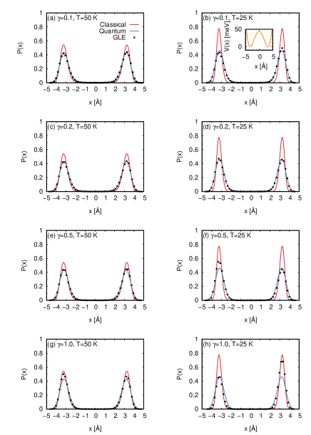
Figure 1: Probability density of a hydrogen atom in a bistable potential well (see the inset of panel (b)) for $T=50$ K (left panels) and $T=25$ K (right panels) and several values of the dimensionless coupling strength, $\gamma$ (black points with error bars). The probabilities and the errors have been estimated from the position histograms of the corresponding equilibrated GLE simulations. Analytic estimates of the classical (red lines) and quantum (blue lines) probability densities are also reported. The dynamics in the cases of $T=25$ (low temperature) and $\gamma\geq 0.5$ (strong coupling) are not ergodic (see text).

In Fig. 1 we show the probability densities obtained by numerical integration of the quasiclassical complex Langevin equations introduced in Eq. (1) with $K=50$ for the case of the hydrogen mass. The numerical integration provides an accurate solution of the equivalent quasiclassical GLE defined in Eq. (4). Details of the integration algorithm can be found in Ref. Stella et al., 2014. For each value of the temperature, $T$, and the dimensionless coupling strength, $\gamma$, $50$ independent trajectories have been generated to sample the position histograms. Each trajectory is randomly started at rest in either the left or the right minima with equal probability. A time step of $1$ fs and $10^{8}$ steps have been used, while the configurations in the extended phase space $\left(r,p,s_{1}^{\left(k\right)},s_{2}^{\left(k\right)}\right)$ have been recorded every $10^{4}$ steps. In each panel, we have also indicated the classical probability density, $P_{cl}\left(x\right)\propto\exp\left(-V\left(x\right)/k_{B}T\right)$, and the quantum probability density, $P_{q}\left(x\right)\propto\sum_{n}\left|\phi_{n}\left(x\right)\right|^{2}\exp\left(-E_{n}/k_{B}T\right)$, where $\phi_{n}$ and $E_{n}$ are the eigenvectors and eigenvalues of the Hamiltonian operator $H=-\left(\hbar^{2}/2m\right)\nabla^{2}+V\left(x\right)$.

From the results shown in the different panels of Fig. 1, we can conclude that the quasiclassical GLE is rather accurate in modelling the quantum probability density when the temperature is not too low and the coupling is not too strong. This conclusion agrees with previous observations.Ceriotti et al. (2009) The capability of a quantum GLE scheme based on the QFDT to model the quantum delocalisation in a moderately anharmonic potential has been exploited to improve the convergence of path-integral molecular dynamics.Ceriotti et al. (2009, 2011) Discrepancies at low temperature are due to the lack of ergodicity which follows a reduced transition rate, $\kappa_{gle}$ (see Sec. IV). Discrepancies in the strong coupling regime are due to the non-negligible corrections to the quantum probability density caused by the system-bath interaction.Riseborough et al. (1985) A detailed assessment of these corrections depends on the characterisation of the persistent oscillation of a Debye bath (see above) and it is therefore left to a future publication. In fact, the main conclusions about the transition rate in the strong coupling regimes (see Sec. IV) do not depend on the detailed assessment of these corrections.

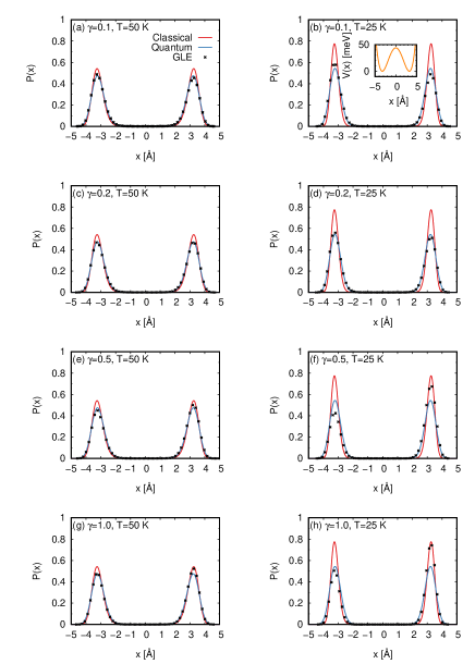
Figure 2: Probability density of a deuterium atom in a bistable potential well (see the inset of panel (b)) for $T=50$ K (left panels) and $T=25$ K (right panels) and several values of the dimensionless coupling strength, $\gamma$ (black points with error bars). The probabilities and the errors have been estimated from the position histograms of the corresponding equilibrated GLE simulations. Analytic estimates of the classical (red lines) and quantum (blue lines) probability densities are also reported. The dynamics in the cases of $T=25$ (low temperature) and $\gamma\geq 0.5$ (strong coupling) are not ergodic (see text).

To investigate the isotope effect, in Fig. 2 we show the probability densities obtained by numerical integration of the quasiclassical complex Langevin equations for a deuterium atom. The same trends with decreasing $T$ and increasing $\gamma$ are observed, even if the quantum probability densities are more localised and the ergodicity breaking is then more severe.

IV Transition rates

The transition rate, $\kappa$, has been estimated from the decay of the position autocorrelation functionGillan (1987)

$$\left\langle r\left(t\right)r\left(t^{\prime}\right)\right\rangle\sim e^{-2\kappa_{gle}\left(t-t^{\prime}\right)}$$ (33)

sampled at $T=13$, $16$, $20$, $25$, $31$, $40$, $50$, $63$, $79$, $100$, $126$, $159$, $200$ K and $\gamma=0.1$, $0.2$, $0.5$, $1.0$. The remaining simulation parameters are the same as for the trajectories used to investigate the probability density (See Sec. III).

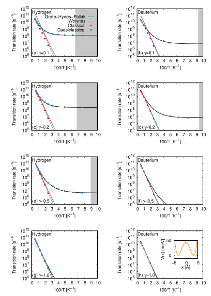
Figure 3: Classical and quasiclassical GLE transition rates of a hydrogen (left panels) or deuterium (right panels) atom in a bistable potential (see the inset of panel (h)) as a function of the inverse temperature for several values of the dimensionless coupling strength, $\gamma$. For comparison, the analytic estimates from the Grote-Hynes-Pollak, Eq. (34), and the Wolynes, Eq. (37), formulae are also reported. The black lines are fits of the quasiclassical GLE results (see Eq. (41)) and the regions for which $T<T_{c}$ are shaded (see Eq. (38)).

In Fig. 3 we show the Arrhenius plots for the different values of the dimensionless coupling strength in the case of the hydrogen mass (left panels) or in the case of the deuterium mass (right panels). The transition rates obtained from the numerical solution of the quasiclassical GLE saturate at very low temperature, while the transition rates from the classical GLE (obtained by fixing $h\left(\omega\right)=1$ in Eq. (1)) display the familiar linear behaviour.

In all the panels of Fig. 3 we also show the analytic estimates of the classical transition rate (Grote-Hynes-PollakGrote and Hynes (1980); Pollak (1986a))

$$\kappa_{ghp}\left(T\right)=\left(\frac{\omega_{ghp}}{\omega_{b}}\right)\kappa_{tst}\left(T\right)\;,$$ (34)

where $-i\omega_{b}$ is the imaginary frequency of the barrier top (i.e., $-m\omega_{b}^{2}$ is the second derivative of the potential at the barrier top) and

$$\kappa_{tst}\left(T\right)=\left(\frac{\Omega_{0}}{2\pi}\right)e^{-\frac{V_{b}}{k_{B}T}}$$ (35)

is the bare estimate of the transition state theory.Eyring (1935) In the case of a Debye bath, the Grote-Hynes-Pollak imaginary frequency, $i\omega_{ghp}$, is given by the positive solution of the equation

$$\omega_{b}^{2}-\omega_{gph}^{2}\left[1+\frac{2\Gamma}{\pi m\omega_{ghp}}\arctan\left(\frac{\omega_{D}}{\omega_{ghp}}\right)\right]=0\;.$$ (36)

The numerical values of $\omega_{ghp}$ are reported in Table 1, for the case of the hydrogen mass, or in Table 2 in the case of the deuterium mass.

The quantum transition rate (WolynesWolynes (1981); Pollak (1986b)) is approximated asBell (1959)

$$\kappa_{w}\left(T\right)\approx\left(\frac{\hbar\omega_{ghp}}{2k_{B}T}\right)\frac{\kappa_{tst}\left(T\right)}{\sin\left(\frac{\hbar\omega_{ghp}}{2k_{B}T}\right)}\approx\left[1+\frac{1}{24}\left(\frac{\hbar\omega_{ghp}}{k_{B}T}\right)^{2}\right]\kappa_{tst}\left(T\right)\;.$$ (37)

The agreement between the Grote-Hynes-Pollak predictions and the classical GLE is very good in all cases, except the very weak, i.e., $\gamma=0.1$, coupling regime. A disagreement is expected in this case since the transitions are limited more by energy diffusion than spatial diffusion (the Kramers turnover problem).Hänggi et al. (1990) Corrections to Eq. (34) are known,Mel’nikov and Meshkov (1986); Grabert (1988); Pollak et al. (1989) but are not relevant in the strong coupling regime.

The quasiclassical GLE rates are in clear quantitative disagreement with the Wolynes predictions in all cases, except the very strong, i.e., $\gamma=1.0$, coupling regime. In particular, the quasiclassical GLE rates saturate at a temperature well above the so-called critical temperature,

$$T_{c}=\frac{\hbar\omega_{ghp}}{2\pi k_{B}}\;,$$ (38)

at which Eq. (37) displays an (apparent) divergence.Grabert et al. (1987); Hänggi and Hontscha (1988, 1991)

Following Miller,Miller (1977) one can use the critical temperature, $T_{c}$, to characterise the tunnelling through the barrier top, approximated as $V\left(r\right)\approx V_{b}-\frac{1}{2}m\omega_{b}^{2}r^{2}$. In this case, the tunnelling probability is

$$P_{t}\left(E\right)=\frac{1}{1+\exp\left(\frac{2\pi\left(V_{b}-E\right)}{\hbar\omega_{b}}\right)}=\frac{1}{1+\exp\left(\frac{V_{b}-E}{k_{B}T_{c}}\right)}\;,$$ (39)

where $E$ is the total energy of the system. By means of Eq. (39), the quantum transition rate is estimated as

$$\kappa_{m}\left(T\right)=\left(\frac{\Omega_{0}}{2\pi K_{B}T}\right)\int_{-\infty}^{\infty}\mbox{d}E\;e^{-\frac{E}{k_{B}T}}P_{t}\left(E\right)=\left(\frac{\hbar\omega_{b}}{2k_{B}T}\right)\frac{\kappa_{tst}\left(T\right)}{\sin\left(\frac{\hbar\omega_{b}}{2k_{B}T}\right)}\;.$$ (40)

Note that Eq. (37) and Eq. (40) differ only in the choice of imaginary frequency of the barrier top. In fact, we have that $\omega_{ghp}\to\omega_{b}$ in the limit of $\gamma\to 0$ (see Eq. (36) and Eq. (29)).

At low temperature, $k_{B}T\ll V_{b}$, assuming that the zero-point energy is negligible, $\hbar\Omega_{0}/2\ll V_{b}$, one can substitute $E\approx 0$ into Eq. (39) to approximate $P_{t}\left(0\right)\approx e^{-\frac{V_{b}}{k_{B}T_{c}}}$. As a consequence, tunnelling is expected to be the dominant transition mechanism for $T<T_{c}$. The numerical values of $T_{c}$ are reported in Table 1 or Table 2. The critical temperature, $T_{c}$, is a function of both the dimensionless coupling strength, $\gamma$, and the mass, $m$, through its dependence on $\omega_{ghp}$. The regions corresponding to $T<T_{c}$ have been shaded in the panels of Fig. 3.

To help interpret the quasiclassical GLE results, we model the quasiclassical transition rate by means of the function

$$\kappa_{fit}\left(T\right)=\left(\frac{A}{2\pi}\right)\exp\left(-\frac{B}{h\left(\omega^{\ddagger}\right)k_{B}T}\right)\;,$$ (41)

where $A$, $B$, and $\omega^{\ddagger}$ are adjustable parameters, the values of which are reported in Table 1,

$\gamma$	$A$ [fs-1]	$B$ [eV]	$\omega^{\ddagger}$ [fs-1]	$T_{q}$ [K]	$T_{c}$ [K]	$\omega_{ghp}$ [fs-1]
$0.1$	$0.00157$	$0.0359$	$0.0144$	$67.1$	$15.1$	$0.0124$
$0.2$	$0.00503$	$0.0371$	$0.0139$	$62.9$	$14.6$	$0.0120$
$0.5$	$0.00916$	$0.0403$	$0.0097$	$40.5$	$11.2$	$0.0092$
$1.0$	$0.00439$	$0.0426$	$0.0040$	$15.9$	$4.6$	$0.0038$

Table 1: Numerical values of the parameters, $A$, $B$, and $\omega^{\ddagger}$ (errors on the last digit) appearing in Eq. (41) as a function of the dimensionless coupling strength, $\gamma$, along with the estimates of the quantum temperature, $T_{q}$, the critical temperature, $T_{c}$, and the Grote-Hynes-Pollak frequency, $\omega_{ghp}$, in the case of the hydrogen mass.

or Table 2.

$\gamma$	$A$ [fs-1]	$B$ [eV]	$\omega^{\ddagger}$ [fs-1]	$T_{q}$ [K]	$T_{c}$ [K]	$\omega_{ghp}$ [fs-1]
$0.1$	$0.00157$	$0.0360$	$0.0105$	$48.8$	$10.6$	$0.0087$
$0.2$	$0.00502$	$0.0386$	$0.0101$	$43.8$	$10.0$	$0.0083$
$0.5$	$0.00699$	$0.0431$	$0.0064$	$25.0$	$6.6$	$0.0055$
$1.0$	$0.00236$	$0.0434$	$0.0029$	$11.1$	$2.3$	$0.0019$

Table 2: Numerical values of the parameters, $A$, $B$, and $\omega^{\ddagger}$ (errors on the last digit) appearing in Eq. (41) as a function of the dimensionless coupling strength, $\gamma$, along with the estimates of the quantum temperature, $T_{q}$, the critical temperature, $T_{c}$, and the Grote-Hynes-Pollak frequency, $\omega_{ghp}$, in the case of the deuterium mass.

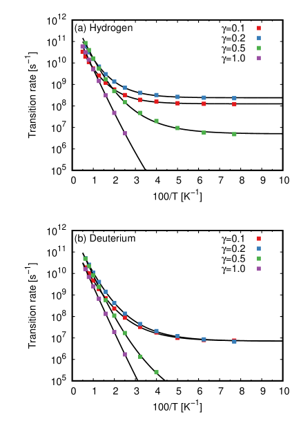
Figure 4: Quasiclassical GLE transition rates of a hydrogen (panel (a)) or deuterium (panel (b)) atom in a bistable potential as a function of the inverse temperature (Arrhenius plots) for several values of the dimensionless coupling strength, $\gamma$. The black lines are fits of the quasiclassical GLE results (see Eq. (41)).

The global accuracy of these fits can be better appreciated from Fig. 4, where we have reported only the quasiclassical GLE rates. By interpreting the exponential in Eq. (41) as a Boltzmann factor, we can define an effective quantum temperature, $T_{q}$, so that

$$\frac{V_{b}}{k_{B}T_{q}}=\frac{B}{\frac{\hbar\omega^{\ddagger}}{2}}\;.$$ (42)

The numerical values of $T_{q}$ are reported in Table 1, for the case of the hydrogen mass, or Table 2 in the case of the deuterium mass. The quantum temperature can be used to assess the validity of discrepancy between the quasiclassical GLE and the analytic predictions (see Sec. V).

V Discussion

The quasiclassical GLE formalism considered in this article does not include tunnelling.Eckern et al. (1990) It is then not surprising that it fails to model the transition rates in the deep quantum regime. On the other hand, it is not immediately clear why such a formalism overestimates instead of underestimating — as naively suggested by the absence of tunnelling — the quantum transition rates. In this Section we attempt an answer by discussing in more detail the results of Sec. III and IV.

First of all, from the results shown in Figs. 1 and 2, we know that the quasiclassical GLE reproduces rather accurately the probability density, at least close to the potential minima. In the limit of $T\to 0$ and $\gamma\to 0$, the quantum fluctuations close to the minima are entirely due to the zero-point motion which can be characterised by the effective temperature $T_{zp}=\hbar\Omega_{0}/2k_{B}$. In particular, we have that $T_{zp}=136$ K in the case of the hydrogen mass or $T_{zp}=96.2$ K in the case of the deuterium mass. Those temperatures are much larger than $T_{q}$ and $T_{c}$ in both cases. Given the good agreement between the classical GLE rates and the Grote-Hynes-Pollak formula for moderate to strong system-bath coupling, we can also exclude a large contribution from the finite height of the barrier (the condition $k_{B}T_{zp}\ll V_{b}$ is satisfied). It is then plausible that the discrepancies between the quasiclassical GLE and the analytic predictions originate from an incorrect sampling of the region close to the barrier top.

The quasiclassical GLE considered in this article provides an inherently thermal (i.e., classical) description of the random forces, although the physical temperature is weighted by a correcting factor, $h\left(\omega\right)$, which depends on the frequency of the oscillations, $\omega$, to mimic the quantum fluctuations. In practise, the quantum temperature, $T_{q}$, can be used to estimate the effective temperature close to the barrier top.

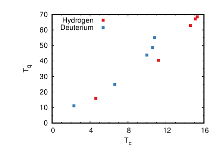
Figure 5: Correlation between the effective quantum temperature, $T_{q}$, and the critical temperature, $T_{c}$.

Interestingly, we observe that the ratio between $T_{q}$ and $T_{c}$ is a relatively constant function of $\gamma$ and $m$ (between $0.4$ and $0.5$, see Fig. 5). Our results are in agreement with the findings of Eckern et al. (see Ref. Eckern et al., 1990, in particular at the end of Sec. 2.3). This observation suggests that, despite the quantitative discrepancy between the quasiclassical GLE and the analytic predictions, the functional dependence of $\kappa_{gle}\left(T\right)$ on both $\gamma$ and $m$ is qualitatively correct. In particular, the isotope effect and the convergence of the quantum and classical transition rates in the strong coupling limit are in good qualitative agreement with the analytic predictions.Pollak (1986c); Grabert et al. (1987)

VI Conclusions

In this article, we have completed the GLE formalism introduced in Ref. Stella et al., 2014 to include the quantum delocalisation at very low temperature. Our results confirm the applicability of this formalism to model the equilibrium properties (e.g., the probability density) of a bistable system coupled to a Debye bath. In particular, the quasiclassical GLE formalism equally applies to both the weak and strong coupling regimes.

The quantitative discrepancy between the quasiclassical GLE and the analytic predictions for the quantum transition rates has been rationalised as the consequence of an incorrect sampling close to the barrier top. In particular, the quasiclassical GLE predicts a saturation of the transition rate at an effective quantum temperature, $T_{q}$, which is roughly twice as large as the expected critical temperature, $T_{c}$. Since the value of $T_{c}$ depends on the imaginary frequency of the barrier top (see Eq. (38)), we can conclude that the quasiclassical GLE effectively samples a different imaginary frequency. On the other hand, the quasiclassical GLE accurately samples the quantum probability distribution (at least for weak system-bath interaction) close to the minima of the potential wells. Since the ratio between $T_{q}$ and $T_{c}$ is roughly constant, the functional dependence of $\kappa_{gle}\left(T\right)$ on both the system-bath coupling strength, $\gamma$, and the particle mass, $m$, is also qualitatively correct. This qualitative agreement includes the isotope effect and the convergence of the quantum and classical transition rates in the strong coupling limit.

Our results shed more light on the domain of applicability of a real-time GLE approach to model the relaxation of quantum dissipative system. The simple quasiclassical approach considered in this article ignores both the quantum corrections to the force field Banerjee et al. (2002a); Barik et al. (2003a, b); Banerjee et al. (2004) and the proper treatment of the quantum fluctuations by means of the path integral formalismCeriotti et al. (2009, 2011); Richardson and Althorpe (2009); Hele et al. (2015). However, it is surprisingly accurate in the limit of strong system-bath interaction, at a computational cost essentially equal to that of its classical counterpart.

References

- Zwanzig (1961) R. Zwanzig, Phys. Rev. 124, 983 (1961).
- Mori (1965a) H. Mori, Prog. Theor. Phys. 33, 423 (1965a).
- Mori (1965b) H. Mori, Prog. Theor. Phys. 34, 399 (1965b).
- Zwanzig (1973) R. Zwanzig, J. Stat. Phys. 9, 215 (1973).
- Lemons and Gythiel (1997) D. S. Lemons and A. Gythiel, Am. J. Phys. 65, 1079 (1997).
- Kubo (1966) R. Kubo, Rep. Prog. Phys. 29, 255 (1966).
- Zwanzig (2001) R. Zwanzig, Nonequilibrium Statistical Mechanics (Oxford University Press, 2001).
- Kramers (1940) H. Kramers, Physica 7, 284 (1940).
- Hänggi et al. (1990) P. Hänggi, P. Talkner, and M. Borkovec, Rev. Mod. Phys. 62, 251 (1990).
- Pollak (1986a) E. Pollak, J. Chem. Phys. 85, 865 (1986a).
- Pollak et al. (1989) E. Pollak, H. Grabert, and P. Hn̈ggi, J. Chem. Phys. 91, 4073 (1989).
- Tucker et al. (1991) S. C. Tucker, M. E. Tuckerman, B. J. Berne, and E. Pollak, J. Chem. Phys. 95, 5809 (1991).
- Carmeli and Nitzan (1982) B. Carmeli and A. Nitzan, Phys. Rev. Lett. 49, 423 (1982).
- Carmeli and Nitzan (1983) B. Carmeli and A. Nitzan, J. Chem. Phys. 79, 393 (1983).
- Marchesoni and Grigolini (1983) F. Marchesoni and P. Grigolini, J. Chem. Phys. 78, 6287 (1983).
- Ford et al. (1965) G. W. Ford, M. Kac, and P. Mazur, J. Math. Phys. 6, 504 (1965).
- Benguria and Kac (1981) R. Benguria and M. Kac, Phys. Rev. Lett. 46, 1 (1981).
- Ford and Kac (1987) G. W. Ford and M. Kac, J. Stat. Phys. 46, 803 (1987).
- Ford et al. (1988a) G. W. Ford, J. T. Lewis, and R. F. O’Connell, Phys. Rev. B 37, 4419 (1988a).
- Pollak (1986b) E. Pollak, Chem. Phys. Lett. 127, 178 (1986b).
- Pollak (1986c) E. Pollak, Phys. Rev. A 33, 4244 (1986c).
- Ford et al. (1988b) G. Ford, J. Lewis, and R. O’Connell, Phys. Lett. A 128, 29 (1988b).
- Caldeira and Leggett (1981) A. O. Caldeira and A. J. Leggett, Phys. Rev. Lett. 46, 211 (1981).
- Caldeira and Leggett (1983a) A. Caldeira and A. Leggett, Physica A 121, 587 (1983a).
- Caldeira and Leggett (1983b) A. Caldeira and A. Leggett, Ann. Phys. 149, 374 (1983b).
- Grabert et al. (1988) H. Grabert, P. Schramm, and G.-L. Ingold, Phys. Rep. 168, 115 (1988).
- Note (1) Following DiracDirac (1926), -numbers are “classical numbers” which always commute (e.g., complex numbers), while -numbers are “quantum numbers” which do not commute in general (e.g., linear operators).
- Schmid (1982) A. Schmid, J. Low Temp. Phys. 49, 609 (1982).
- Eckern et al. (1990) U. Eckern, W. Lehr, A. Menzel-Dorwarth, F. Pelzer, and A. Schmid, J. Stat. Phys. 59, 885 (1990).
- Stockburger and Grabert (2002) J. T. Stockburger and H. Grabert, Phys. Rev. Lett. 88, 170407 (2002).
- Barik et al. (2003a) D. Barik, B. C. Bag, and D. S. Ray, J. Chem. Phys. 119, 12973 (2003a).
- Banerjee et al. (2004) D. Banerjee, B. C. Bag, S. K. Banika, and D. S. Ray, J. Chem. Phys. 120, 8960 (2004).
- Dammak et al. (2009) H. Dammak, Y. Chalopin, M. Laroche, M. Hayoun, and J.-J. Greffet, Phys. Rev. Lett. 103, 190601 (2009).
- Kantorovich et al. (2016) L. Kantorovich, H. Ness, L. Stella, and C. D. Lorenz, Phys. Rev. B 94, 184305 (2016).
- Stella et al. (2014) L. Stella, C. D. Lorenz, and L. Kantorovich, Phys. Rev. B 89, 134303 (2014).
- Banerjee et al. (2002a) D. Banerjee, B. C. Bag, S. K. Banik, and D. S. Ray, Phys. Rev. E 65, 021109 (2002a).
- Banerjee et al. (2002b) D. Banerjee, S. K. Banik, B. C. Bag, and D. S. Ray, Phys. Rev. E 66, 051105 (2002b).
- Grabert et al. (1987) H. Grabert, P. Olschowski, and U. Weiss, Phys. Rev. B 36, 1931 (1987).
- Cortes et al. (1985) E. Cortes, B. J. West, and K. Lindenberg, J. Chem. Phys. 82, 2708 (1985).
- Ceriotti et al. (2009) M. Ceriotti, G. Bussi, and M. Parrinello, Phys. Rev. Lett. 103, 030603 (2009).
- Note (2) In fact, includes a “polaronic” correction due to the system-bath interaction. For the sake of simplicity, we do not treat this correction explicitly in the rest of this article and we treat as if it was independent of the system-bath coupling strength.
- Note (3) Higher order correlations function are computed by means of the Wick’s theorem.
- Note (4) The quantum weight is the ratio between the internal energy of an independent bosonic oscillator, , and the internal energy of an independent classical oscillator, , of equal frequency, . In both cases, “independent” means “in the limit of vanishing small system-bath interaction”.
- Kantorovich and Rompotis (2008) L. Kantorovich and N. Rompotis, Phys. Rev. B 78, 094305 (2008).
- Ness et al. (2015) H. Ness, L. Stella, C. D. Lorenz, and L. Kantorovich, Phys. Rev. B 91, 014301 (2015).
- Ness et al. (2016) H. Ness, A. Genina, L. Stella, C. D. Lorenz, and L. Kantorovich, Phys. Rev. B 93, 174303 (2016).
- Gottwald et al. (2015) F. Gottwald, S. Karsten, S. D. Ivanov, and O. Kühn, The Journal of Chemical Physics 142, 244110 (2015).
- Gottwald et al. (2016) F. Gottwald, S. D. Ivanov, and O. Kühn, The Journal of Chemical Physics 144, 164102 (2016).
- Note (5) For the sake of simplicity, here we assume that the are trivial (i.e., constant) function of .
- Kemeny et al. (1986) G. Kemeny, S. D. Mahanti, and T. A. Kaplan, Phys. Rev. B 34, 6288 (1986).
- Note (6) In fact, in this work we have preferred the “BAOAB” algorithm of Leimkuhler and Matthews which is known to give better estimates of the confrontational averages.Leimkuhler and Matthews (2013) This choice implies a simple rearrangements of the split algorithm employed in Ref. \rev@citealpnumStella2014.
- Ceriotti et al. (2011) M. Ceriotti, D. E. Manolopoulos, and M. Parrinello, J. Chem. Phys. 134, 084104 (2011).
- Riseborough et al. (1985) P. S. Riseborough, P. Hanggi, and U. Weiss, Phys. Rev. A 31, 471 (1985).
- Gillan (1987) M. Gillan, J. Phys. Condens. Matter 20, 3621 (1987).
- Grote and Hynes (1980) R. F. Grote and J. T. Hynes, J. Chem. Phys. 73, 2715 (1980).
- Eyring (1935) H. Eyring, J. Chem. Phys. 3, 107 (1935).
- Wolynes (1981) P. G. Wolynes, Phys. Rev. Lett. 47, 968 (1981).
- Bell (1959) R. P. Bell, Trans. Faraday Soc. 55, 1 (1959).
- Mel’nikov and Meshkov (1986) V. Mel’nikov and S. V. Meshkov, J. Chem. Phys. 855, 1018 (1986).
- Grabert (1988) H. Grabert, Phys. Rev. Lett. 61, 1683 (1988).
- Hänggi and Hontscha (1988) P. Hänggi and W. Hontscha, J. Chem. Phys. 88, 4094 (1988).
- Hänggi and Hontscha (1991) P. Hänggi and W. Hontscha, Ber. Bunsenges. Phys. Chem. 95, 379 (1991).
- Miller (1977) W. H. Miller, Farad. Discuss. 62, 40 (1977).
- Note (7) One can set to reduce the number of adjustable parameters, but the fits generally get worse. The difference between and is due to the quantum fluctuations.Pollak (1986c).
- Barik et al. (2003b) D. Barik, S. K. Banik, and D. S. Ray, J. Chem. Phys. 119, 680 (2003b).
- Richardson and Althorpe (2009) J. O. Richardson and S. C. Althorpe, J. Chem. Phys. 131, 214106 (2009).
- Hele et al. (2015) T. J. H. Hele, M. J. Willatt, A. Muolo, and S. C. Althorpe, J. Chem. Phys. 142, 191101 (2015).
- Dirac (1926) P. A. M. Dirac, Proc. R. Soc. Lond. A 110, 561 (1926).
- Leimkuhler and Matthews (2013) B. Leimkuhler and C. Matthews, J. Chem. Phys. 138, 174102 (2013).