Pion radiative weak decay from the instanton vacuum

Abstract

We investigate the vector and axial-vector form factors for the pion radiative weak decays $\pi^{+}\to e^{+}\nu_{e}\gamma$ and $\pi^{+}\to e^{+}\nu_{e}e^{+}e^{-}$, based on the gauged effective chiral action from the instanton vacuum in the large $N_{c}$ limit. The nonlocal contributions, which arise from the gauging of the action, enhance the vector form factor by about $20\,\%$, whereas the axial-vector form factor is reduced by almost $30\,\%$. Both the results for the vector and axial-vector form factors at the zero momentum transfer are in good agreement with the experimental data. The dependence of the form factors on the momentum transfer is also studied. The slope parameters are computed and compared with other works.

I Introduction

Pion radiative decay $\pi^{+}\to e^{+}\nu_{e}\gamma$ provides rich information on the structure of the pion. The decay amplitude for the pion radiative decay consists of two part, i.e., the structure-dependent (SD) part containing the vector and axial-vector form factors of the pion and the inner Bremsstrahlung (IB) part Vaks:1958 ; Bludman:1960 ; Bryman:1982et ; PDG . The advantage of studying $\pi^{+}\to e^{+}\nu_{e}\gamma$ decay over $\pi^{+}\to\mu^{+}\nu_{\mu}\gamma$ is that the IB part is suppressed in the $\pi^{+}\to e^{+}\nu_{e}\gamma$ decay Bryman:1982et ; PDG , whereas the corresponding SD part is enhanced due to the helicity. Thus, the $\pi^{+}\to e^{+}\nu_{e}\gamma$ decay allows one to get access to the structure of the pion experimentally. The vector form factor $F_{V}$ is related to the decay rate of the $\pi^{0}\to\gamma\gamma$ decay Vaks:1958 ; Gershtein:1955fb by the vector current conservation, so it was easier to find it using the lifetime of $\pi^{0}$. On the other hand, it took many years to measure unambiguously the axial-vector form factors Depommier:1962jpa ; Depommier:1963zza ; Stetz:1977ge ; Bay:1986kf ; Piilonen:1986bv ; Egli:1986nk ; Egli:1989vu ; Bolotov:1990yq ; Frlez:2003pe . Some years ago, PIBETA Collaboration Bychkov:2008ws conducted a precise measurement of the pion weak form factors, reporting the values of the vector and axial-vector form factors respectively as $F_{V}(0)=0.0258(17)$ and $F_{A}(0)=0.0117(17)$. The slope of the vector form factor was also measured: $a_{V}=0.10(6)$, which is defined in the parametrization of the vector form factor $F_{V}(q^{2})=F_{V}(0)/(1-a_{V}q^{2}/m_{\pi}^{2})$ near $q^{2}\approx 0$. There is yet the second axial-vector form factor which comes into play when the photon is virtual. The SINDRUM Collaboration Egli:1989vu reported the first measurement of the decay $\pi^{+}\to e^{+}\nu_{e}e^{+}e^{-}$ in which the off-mass-shell photon decays into $e^{+}e^{-}$, and yielded the second axial-vector form factor to be $R_{A}(0)=0.059_{-0.008}^{+0.009}$.

The vector and axial-vector form factors for the pion radiative decay were studied in chiral perturbation theory Holstein:1986uj ; Bijnens:1996wm ; Geng:2003mt ; Mateu:2007tr ; Unterdorfer:2008zz , since the experimental data on the axial-vector form factor can be used to determine a part of the low-energy constants that encode information on nonperturbative quark-gluon dynamics. These form factors have been also investigated within various theoretical frameworks: For example, quantum chromodynamics (QCD) sum rules Nasrallah:1981rn , the nonlocal Nambu-Jona-Lasinio (NJL) model Dumm:2010hh ; GomezDumm:2012qh , and in the light-front quark model Chen:2010ue . Since the photon can be virtual, it is of interest to examine the dependence of the form factors on the momentum transfer. Chiral perturbation theory predicts very mild dependence on the momentum transfer in the range of $0\leq q^{2}\leq 0.018\,\mathrm{GeV}^{2}$ Bijnens:1996wm . On the other hand, the results for the vector and axial-vector form factors from the light-front quark model start to rise near $q^{2}=0$ and then fall off drastically as $q^{2}$ increases Chen:2010ue . On the contrary, the nonlocal NJL model GomezDumm:2012qh predicted only the $q^{2}$ dependence of the vector form factor. The results monotonically decrease as $q^{2}$ increases. Thus, it is of great importance to investigate the weak form factors for the pion radiative decay and compare them with those from other works.

In the present work, we study the three weak form factors of the pion, i.e., the vector form factor, the axial-vector form factor, and the second axial-vector form factor, based on the gauged effective chiral action (E$\chi$A) from the instanton vacuum Diakonov:1985eg ; Diakonov:2002fq ; Musakhanov:2002xa ; Kim:2004hd ; Kim:2005jc ; Goeke:2007nc ; Goeke:2007bj . Since the spontaneous breakdown of chiral symmetry is naturally realized from the instanton vacuum, it provides a good framework to investigate properties of the pion, i.e. of the pseudo-Nambu-Goldstone bosons. The quark acquires the dynamical quark mass that is momentum-dependent through the quark zero modes in the instanton background. Moreover, there are only two parameters in this approach, namely, the average instanton size $\bar{\rho}\approx 1/3$ fm and average interinstanton distance $\bar{R}\approx 1$ fm. Since the average size of instantons is considered as a normalization point equal to $\bar{\rho}^{-1}\approx 0.6$ GeV, we can use the model for computing any observables of hadrons and compare the results with those from other theoretical framework such as $\chi$PT and lattice QCD, in particular, when a specific scale is involved. These values of the $\bar{\rho}$ and $\bar{R}$ were determined many years ago theoretically Diakonov:1985eg ; Diakonov:2002fq as well as phenomenologically Shuryak:1981ff ; Schafer:1996wv . They were also confirmed by various lattice works Chu:1994vi ; Negele:1998ev ; DeGrand:2001tm . In Ref. Cristoforetti:2006ar , the QCD vacuum was simulated in the interacting instanton liquid model and $\bar{\rho}\approx 0.32\,\mathrm{fm}$ and $\bar{R}\approx 0.76\,\mathrm{fm}$ were obtained with the finite current quark mass taken into account.

Since we consider the pion mass, we need to introduce the current quark mass. Musakhanov Musakhanov:1998wp ; Musakhanov:2002vu improved the E$\chi$A derived by Diakonov and Petrov Diakonov:1985eg , including the current quark mass. In fact, this improvement plays an essential role in understanding the QCD vacuum in the presence of the finite mass of the current quark. In Ref. Nam:2006ng , it was shown that the improved E$\chi$A properly described the dependence of the quark and gluon condensates on the current quark mass. Furthermore, the nonlocality arising from the momentum-dependent dynamical quark mass is known to bring out the breakdown of the Ward-Takahashi (WT) identities, that is, the current nonconservation Chretien:1954we ; Pobylitsa:1989uq ; Bowler:1994ir ; Musakhanov:1996cv . In Refs. Musakhanov:2002xa ; Kim:2004hd , the gauged E$\chi$A was derived from the instanton vacuum, which satisfies the WT identities. We will employ this action in the present work to investigate the weak form factors for pion radiative decay.

The structure of the present work is sketched as follows: In Section II, we will define the three weak form factors of the pion, which will be related to the transition matrix elements of the vector and axial-vector currents. In Section III, we briefly explain the gauged E$\chi$A. In Section IV, we derive the vector and axial-vector form factors, using the gauged E$\chi$A. In Section V, we present the numerical results of the three form factors and discuss them. The final Section is devoted to summary and conclusion.

II Weak form factors of the $\pi^{+}\to e^{+}\nu\gamma$ decay

The SD part of the pion radiative decay amplitude consists of the weak transition form factors of the pion, i.e., the vector form factor $F_{V}(q^{2})$, the axial-vector form factor $F_{A}(q^{2})$, and the second axial-vector form factors $R_{A}(q^{2})$. They are defined in terms of the transition matrix elements of the vector and axial-vector currents as follows

$$\langle\gamma(k)|V_{12}^{\mu}(0)|\pi^{+}(p)\rangle =-\frac{e}{m_{\pi}}\epsilon_{\alpha}^{*}F_{V}(q^{2})\epsilon^{\mu\alpha\rho\sigma}p_{\rho}k_{\sigma},$$ (1)

$$\langle\gamma(k)|A_{12}^{\mu}(0)|\pi^{+}(p)\rangle =ie\epsilon_{\alpha}^{*}\sqrt{2}f_{\pi}\left[-g^{\mu\alpha}+q^{\mu}(q^{\alpha}+p^{\alpha})\frac{F_{\pi}(k^{2})}{q^{2}-m_{\pi}^{2}}\right]$$ (2)

$$\hskip 8.5359pt+i\epsilon_{\alpha}^{*}\frac{e}{m_{\pi}}\left[F_{A}(q^{2})\left(k^{\mu}q^{\alpha}-g^{\mu\alpha}q\cdot k\right)+R_{A}(q^{2})\left(k^{\mu}k^{\alpha}-g^{\mu\alpha}k^{2}\right)\right],$$ (3)

where $|\pi^{+}(p)\rangle$ and $|\gamma(k)\rangle$ stand for the initial pion and the final photon states, the transition vector and axial-vector currents are defined respectively as

$$V_{12}^{\mu}=\bar{\psi}\gamma^{\mu}\frac{\tau_{1}-i\tau_{2}}{2}\psi,\;\;\;A_{12}^{\mu}=\bar{\psi}\gamma^{\mu}\gamma_{5}\frac{\tau_{1}-i\tau_{2}}{2}\psi,$$ (4)

consisting of the quark fields $\psi=(u,\,d)$, the Dirac matrices $\gamma_{\mu}$ and $\gamma_{5}$, and the Pauli matrices $\tau_{i}$ in isospin space. $p$ and $k$ denote respectively the momenta of the pion and the photon, whereas $q$ is the momentum of the lepton pair. The mass of the pion can be obtained from $p^{2}=m_{\pi}^{2}$ with the mass of the pion $m_{\pi}=139.57$ MeV. $F_{V}(q^{2})$ and $F_{A}(q^{2})$ are the vector and axial-vector form factors of the pion respectively. The second axial-vector form factor, $R_{A}(q^{2})$ contributes only when the outgoing photon is virtual($k^{2}\neq 0$). $F_{\pi}(k^{2})$ is the electromagnetic form factor which gives $F_{\pi}(0)=1$. Electromagnetic charge radius $\langle r^{2}_{\pi}\rangle$ and $F_{\pi}(k^{2})$, were already calculated by one of the authors and his collaborator in this model Nam:2007gf .

III Gauged effective chiral action in the presence of external fields

Since we want to compute the weak form factors of pion radiative decay in this work, we introduce all the relvant external fields in the gauge-invariant manner, i.e., the electromagnetic field $v^{\mathrm{em}}$, the vector fields $v$, and the axial-vector fields $a$

$$\mathcal{S}_{\mathrm{eff}}[v^{\mathrm{em}},v,a,\pi]=-\mathrm{Sp}\ln\left[i\,\not{\mathcal{D}}+i\hat{m}+i\sqrt{M(i\,\mathcal{D}^{L})}U^{\gamma_{5}}\sqrt{M(i\,\mathcal{D}^{R})}\right],$$ (5)

where the functional trace $\mathrm{Sp}$ runs over the space-time, color, flavor, and spin spaces. The current quark mass matrix $\hat{m}$ is written as $\mathrm{diag}(m_{u},\,m_{d})=\bar{m}\bm{1}+m_{3}\tau_{3}$ with $\bar{m}=(m_{u}+m_{d})/2$ and $m_{3}=(m_{u}-m_{d})/2$. $\tau_{3}$ is the third component of the Pauli matrix. Note that isospin symmetry is assumed, so $m_{3}=0$. The covariant derivative $\mathcal{D}_{\mu}$ is defined as

$$i\,\mathcal{D}_{\mu}=i\partial_{\mu}+e\hat{Q}\,v^{\mathrm{em}}_{\mu}+\frac{\tau^{a}}{2}v^{a}_{\mu}+\gamma_{5}\frac{\tau^{a}}{2}a^{a}_{\mu}$$ (6)

with the charge operator for the quark fields

$$\hat{Q}=\left(\begin{array}[]{cc}\frac{2}{3}&0\\ 0&-\frac{1}{3}\end{array}\right)=\frac{1}{6}+\frac{1}{2}\tau_{3}.$$ (9)

The left-handed and right-handed covariant derivatives in the momentum-dependent dynamical quark mass $M(i\mathcal{D}_{L,R})$ are defined respectively as

$$i\,\mathcal{D}_{\mu}^{L}=i\partial_{\mu}+e\hat{Q}\,v^{\mathrm{em}}_{\mu}+\frac{\tau^{a}}{2}v^{a}_{\mu}-\gamma_{5}\frac{\tau^{a}}{2}a^{a}_{\mu},\;\;\;i\,\mathcal{D}_{\mu}^{R}=i\partial_{\mu}+e\hat{Q}\,v^{\mathrm{em}}_{\mu}+\frac{\tau^{a}}{2}v^{a}_{\mu}+\gamma_{5}\frac{\tau^{a}}{2}a^{a}_{\mu}.$$ (10)

The momentum-dependent quark mass with the covariant derivatives ensures the gauge invariance of Eq. (5)in the presence of the external fields. In fact, it was shown that the The nonlinear pseudo-Nambu-Goldstone boson field is expressed as

$$U^{\gamma_{5}}=U(x)\frac{1+\gamma_{5}}{2}+U^{\dagger}(x)\frac{1-\gamma_{5}}{2}=\exp\left(\frac{i\gamma_{5}}{f_{\pi}}\bm{\tau}\cdot\bm{\pi}\right),$$ (11)

where $F_{\pi}$ is the pion decay constant. The pion fields are given as

$$\bm{\tau}\cdot\bm{\pi}=\frac{1}{\sqrt{2}}\left(\begin{array}[]{cc}\frac{1}{\sqrt{2}}\pi^{0}&\pi^{+}\\ \pi^{-}&-\frac{1}{\sqrt{2}}\pi^{0}\end{array}\right).$$ (12)

The momentum-dependent dynamical quark mass, which arises from the the quark-zero mode of the Dirac equation with the instanton fields, is given by

$$M_{f}(k)=M_{0}F^{2}(k)f(m_{f}),$$ (13)

where $M_{0}$ is the constituent quark mass at zero quark virtuality, and is determined by the saddle-point equation, resulting in about $350$ MeV Diakonov:1985eg ; Diakonov:2002fq . The form factor $F(k)$ arises from the Fourier transform of the quark zero-mode solution for the Dirac equation with the instanton and has the following form:

$$F(k)=2\tau\left[I_{0}(\tau)K_{1}(\tau)-I_{1}(\tau)K_{0}(\tau)-\frac{1}{\tau}I_{1}(\tau)K_{1}(\tau)\right],$$ (14)

where $\tau\equiv\frac{|k|\bar{\rho}}{2}$. $I_{0,1}$ and $K_{0,1}$ denote the modified Bessel functions. In addition to this original form, we also use the dipole-type parametrization of $F(k)$ defined by

$$F(k)=\frac{2\Lambda^{2}}{2\Lambda^{2}+k^{2}}$$ (15)

with $\Lambda=1/\bar{\rho}$. As mentioned in Introduction already, the average size of the instanton $\bar{\rho}$ was determined either phenomenonlogically Shuryak:1981ff ; Schafer:1996wv or theoretically Diakonov:1985eg ; Diakonov:2002fq . In the large $N_{c}$ limit, the value of $\bar{\rho}$ was determined to be $\bar{\rho}\simeq 0.33$ fm Diakonov:1985eg ; Diakonov:2002fq . When one considers the $1/N_{c}$ meson-loop corrections, $\bar{\rho}$ is modified to be $\bar{\rho}\simeq 0.35$ fm Kim:2004hd ; Kim:2005jc ; Goeke:2007nc ; Goeke:2007bj . Lattice QCD yields similar results $\bar{\rho}=(0.32-0.36)$ fm Chu:1994vi ; Negele:1998ev ; DeGrand:2001tm ; Cristoforetti:2006ar . Since we compute in this work the weak form factors of pion radiative decay in the large $N_{c}$ limit, we will take $\bar{\rho}=0.33$ fm or $\Lambda=600$ MeV. We will compare the results obtained by using the both form factors. The presence of the current quark mass also affects the dynamical one, which was studied in Refs. Musakhanov:1998wp ; Musakhanov:2002vu in detail. The additional factor $f(m_{f})$ describes the $m_{f}$ dependence of the dynamical quark mass, which is defined as Pobylitsa:1989uq ; Musakhanov:2001pc

$$f(m_{f})=\sqrt{1+\frac{m_{f}^{2}}{d^{2}}}-\frac{m_{f}}{d}.$$ (16)

This $m_{f}$-dependent dynamical quark mass yields the gluon condensate that does not depend on $m_{f}$. Pobylitsa considered the sum of all planar diagrams, expanding the quark propagator in the instanton background in the large $N_{c}$ limit Pobylitsa:1989uq . Taking the limit of $N/(VN_{c})\to 0$ leads to $f(m_{f})$. The parameter $d$ is given as $198$ MeV. The $m_{f}$-dependent dynamical quark mass also explains a correct hierarchy of the chiral condensates: $\langle\bar{u}u\rangle\approx\langle\bar{d}d\rangle>\langle\bar{s}s\rangle$ Nam:2006ng .

IV Pion weak form factors

The matrix elements of the vector and axial vector currents in Eq.(3) are related to the three-point correlation function

$$\langle\gamma(k)|\mathcal{W}_{\mu}^{a}(0)|\pi^{b}(p)\rangle=\epsilon^{*}_{\alpha}\int d^{4}xe^{-ik\cdot x}\int d^{4}ye^{ip\cdot y}\mathcal{G}_{\alpha\rho}^{-1}(k)\mathcal{G}_{\pi}^{-1}(p)\langle 0|\{V^{\mathrm{em}}_{\rho}(x)\mathcal{W}_{\mu}^{a}(0)P^{b}(y)\}|0\rangle,$$ (17)

where $\mathcal{W}_{\mu}^{a}$ expresses generically either the vector current or the axial-vector current defined in Eq.(4). The operators in the correlation function represent the electromagnetic current, vector (axial vector) current, and pion-field operators, respectively. $\mathcal{G}_{\alpha\rho}(k)$, $\mathcal{G}_{\pi}(p)$ stand for the propagators of the photon and the pion, respectively. Then, the matrix element (17) can be directly derived from the gauged effective chiral action given in Eq.(5)

$$\langle\gamma(k)|\mathcal{W}_{\mu}^{a}(0)|\pi^{b}(p)\rangle=\epsilon^{*}_{\alpha}\int d^{4}xe^{-ik\cdot x}\int d^{4}ye^{ip\cdot y}\left.\frac{\delta^{3}\mathcal{S}_{\mathrm{eff}}[v^{\mathrm{em}},w,\pi]}{\delta v_{\alpha}^{\mathrm{em}}(x)\delta w_{\mu}^{a}(0)\delta\pi^{b}(y)}\right|_{v^{\mathrm{em}},w,\pi=0}.$$ (18)

The three-point correlation function in Eq.(18) consists of five Feynman diagrams drawn in Fig. 1. In the case of the vector form factor, only diagram (a) contributes to it, whereas all other diagrams vanish because of the trace over spin space. On the other hand, all the diagrams contribute to the axial-vector form factors.

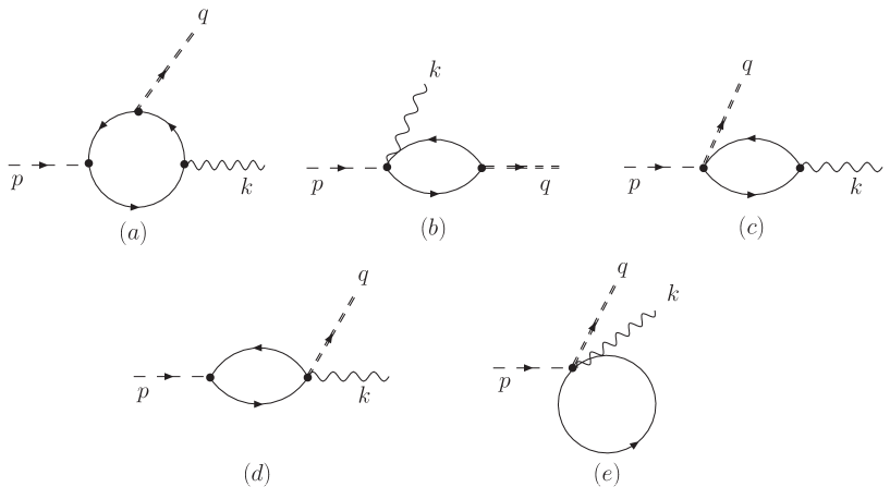
Figure 1: The Feynman diagrams for the pion weak form factors. The dashed line depicts the pion, the dashed double line and the wavy line describe the vector (axial-vector) field and the photon field, respectively. Diagram (a) contains both the local and nonlocal contributions, whereas diagrams (b)-(e) arise from the nonlocal interaction due to the momentum-dependent dynamical quark mass.

Note that diagram (a) contains the contributions from both the local and nonlocal terms, while all other diagrams arise only from the nonlocal terms on account of the momentum-dependent dynamical quark mass.

IV.1 Vector form factor

We first deal with the vector form factor of the pion. Having computed Eq.(18) explicitly, we obtain the matrix element of the vector current ($\mathcal{W}=V$)

$$\langle\gamma(k)|V_{\mu}^{12}|\pi^{+}(p)\rangle =-i\frac{4\sqrt{2}eN_{c}}{3f_{\pi}}\epsilon^{*}_{\alpha}\int\frac{d^{4}l}{(2\pi)^{4}}\frac{\sqrt{M(k_{a})M(k_{b})}}{\mathcal{D}_{a}\mathcal{D}_{b}\mathcal{D}_{c}}\left[\varepsilon_{\mu\alpha\rho\sigma}\left(\bar{M}_{a}k_{b\rho}k_{c\sigma}+\bar{M}_{b}k_{c\rho}k_{a\sigma}+\bar{M}_{c}k_{a\rho}k_{b\sigma}\right)\right.$$ (19)

$$\hskip 11.38092pt-\varepsilon_{\mu\beta\rho\sigma}k_{a\beta}k_{b\rho}k_{c\sigma}\left(\sqrt{M(k_{b})}\sqrt{M_{\alpha}(k_{b})}+\sqrt{M(k_{c})}\sqrt{M_{\alpha}(k_{c})}\right)$$ (20)

$$\hskip 11.38092pt\left.+\varepsilon_{\alpha\beta\rho\sigma}k_{a\beta}k_{b\rho}k_{c\sigma}\left(\sqrt{M(k_{a})}\sqrt{M_{\mu}(k_{a})}+\sqrt{M(k_{c})}\sqrt{M_{\mu}(k_{c})}\right)\right],$$ (21)

where $N_{c}$ denotes the number of colors. $\bar{M}_{i}$ is the sum of the dynamical and current quark masses $\bar{M}_{i}=m+M(k_{i})$. The momenta $k_{i}$ are defined as $k_{a}=l+\frac{q}{2}+\frac{k}{2}$, $k_{b}=l-\frac{q}{2}-\frac{k}{2}$, $k_{c}=l-\frac{q}{2}+\frac{k}{2}$, and $q=p-k$. $\mathcal{D}_{i}$ are given as $\mathcal{D}_{i}=(k_{i}^{2}+\bar{M}_{i}^{2})$. $\sqrt{M_{\mu}(k_{i})}$ represents $\sqrt{M_{\mu}(k_{i})}=\partial\sqrt{M(k_{i})}/\partial k_{i\mu}$. Equation (21) corresponds to diagram (a) in Fig. 1 and there is no contribution from diagrams (b)-(e) in the case of the vector form factor, as mentioned previously. Considering the transverse relation $\epsilon^{*}\cdot p=\epsilon\cdot p=0$, we can extract the vector form factors, comparing Eq.(1) with Eq.(21). Thus, the pion vector form factor is obtained finally as

$$F_{V}(Q^{2})=F_{V}^{\mathrm{local}}(Q^{2})+F_{V}^{\mathrm{NL}}(Q^{2}),$$ (22)

where $F_{V}^{\mathrm{local}}(Q^{2})$ and $F_{V}^{\mathrm{NL}}(Q^{2})$ stand for the local and nonlocal contributions

$$F_{V}^{\mathrm{local}}(Q^{2}) =\frac{4\sqrt{2}N_{c}M_{\pi}}{3f_{\pi}(p\cdot k)^{2}}\int\frac{d^{4}l}{(2\pi)^{4}}\frac{\sqrt{M(k_{a})M(k_{b})}}{D_{a}D_{b}D_{c}}p_{\mu}k_{\nu}\bigg{[}\bar{M}_{a}(k_{b\mu}k_{c\nu}-k_{c\mu}k_{b\nu})$$ (23)

$$\hskip 153.6447pt+\bar{M}_{b}(k_{c\mu}k_{a\nu}-k_{a\mu}k_{c\nu})+\bar{M}_{c}(k_{a\mu}k_{b\nu}-k_{b\mu}k_{a\nu})\Big{]},$$ (24)

$$F_{V}^{\mathrm{NL}}(Q^{2}) =\frac{4\sqrt{2}N_{c}M_{\pi}}{3f_{\pi}(p\cdot k)^{2}}\int\frac{d^{4}l}{(2\pi)^{4}}\frac{\sqrt{M(k_{a})M(k_{b})}}{\mathcal{D}_{a}\mathcal{D}_{b}\mathcal{D}_{c}}\bigg{[}-\Big{(}M^{\prime}(k_{b})+M^{\prime}(k_{c})\Big{)}(p\cdot k)^{2}(\epsilon^{*}\cdot l)(\epsilon\cdot l)$$ (25)

$$\hskip 145.10922pt+\Big{(}M^{\prime}(k_{a})+M^{\prime}(k_{c})\Big{)}(\varepsilon_{\mu\gamma\delta\lambda}l_{\mu}\epsilon_{\gamma}p_{\delta}k_{\lambda})(\varepsilon_{\alpha\beta\rho\sigma}\epsilon^{*}_{\alpha}k_{a\beta}k_{b\rho}k_{c\sigma})\bigg{]},$$ (26)

where $M^{\prime}(k_{i})$ is the derivative of the dynamical quark mass with respective to the squared momentum $M^{\prime}(k_{i})=\partial M^{\prime}(k_{i})/\partial k_{i}^{2}$. The momentum transfer $Q^{2}$ is defined to be positive definite, i.e., $Q^{2}=-q^{2}$.

In fact, one can easily see from Eq. (26) that the terms with $M^{\prime}(k_{i})$ are derived from the expansion of the dynamical quark mass with respect to the covariant detivative given in Eq. (10). Thus, those terms with $M^{\prime}(k_{i})$ are the essential part in obtaining the vector and axial-vector form factors with the corresponding gauge invariance preserved. If the dynamical quark mass is taken to be independent of the quark momentum, then $M^{\prime}(k_{i})$ is equal to zero. It indicates that the nonlocal contributions to the vector form factor vanish such that the results are the same as those derived from the local chiral quark model ($\chi$QM). However, one has to introduce the regularization to tame the divergence arising from the quark loop in the local $\chi$QM. In this sense, the momentum-dependent dynamical quark mass plays also a role of a certain regularization.

IV.2 Axial-vector form factors

The transition matrix element of the axial-vector current ($\mathcal{W}=A$) given in Eq.(3) is obtained as

$$\langle\gamma(k)|A_{\mu}^{12}|\pi^{+}(p)\rangle=-i\frac{4\sqrt{2}eN_{c}}{f_{\pi}}\epsilon^{*}_{\alpha}\int\frac{d^{4}l}{(2\pi)^{4}}\sum^{e}_{i=a}\mathcal{F}^{(i)}_{\mu\alpha},$$ (27)

where $\mathcal{F}^{(i)}_{\mu\alpha}$ corresponds to diagram ($i$), which can be explicitly expressed as

$$\mathcal{F}^{(a)}_{\mu\alpha} =\frac{\sqrt{M(k_{a})M(k_{b})}}{\mathcal{D}_{a}\mathcal{D}_{b}\mathcal{D}_{c}}\left[\delta_{\mu\alpha}\left\{\bar{M}_{a}k_{b}\cdot k_{c}-\bar{M}_{b}k_{c}\cdot k_{a}+\bar{M}_{c}k_{a}\cdot k_{b}+\bar{M}_{abc}\right\}\right.$$ (28)

$$+\left\{-\bar{M}_{a}(k_{b\mu}k_{c\alpha}+k_{c\mu}k_{b\alpha})+\bar{M}_{b}(k_{a\mu}k_{c\alpha}+k_{c\mu}k_{a\alpha})+\bar{M}_{c}(k_{a\mu}k_{b\alpha}-k_{b\mu}k_{a\alpha})\right\}$$ (29)

$$-\left(M^{\prime}(k_{a})k_{a\mu}-M^{\prime}(k_{c})k_{c\mu}\right)\left\{(k_{b}\cdot k_{c}+\bar{M}_{bc})k_{a\alpha}-(k_{c}\cdot k_{a}+\bar{M}_{ca})k_{b\alpha}-(k_{a}\cdot k_{b}+\bar{M}_{ab})k_{c\alpha}\right\}$$ (30)

$$+\left(M^{\prime}(k_{b})k_{b\alpha}+M^{\prime}(k_{c})k_{c\alpha}\right)\left\{-(k_{b}\cdot k_{c}-\bar{M}_{bc})k_{a\mu}+(k_{c}\cdot k_{a}-\bar{M}_{ca})k_{b\mu}-(k_{a}\cdot k_{b}+\bar{M}_{ab})k_{c\mu}\right\}$$ (31)

$$-\left.\left(M^{\prime}(k_{a})k_{a\mu}-M^{\prime}(k_{c})k_{c\mu}\right)\left(M^{\prime}(k_{b})k_{b\alpha}+M^{\prime}(k_{c})k_{c\alpha}\right)\left\{\bar{M}_{a}k_{b}\cdot k_{c}-\bar{M}_{b}k_{c}\cdot k_{a}-\bar{M}_{c}k_{a}\cdot k_{b}-\bar{M}_{abc}\right\}\right],$$ (32)

$$\mathcal{F}^{(b)}_{\mu\alpha} =\frac{\sqrt{M(k_{a})M(k_{b})}}{\mathcal{D}_{a}\mathcal{D}_{c}}\frac{M^{\prime}(k_{b})k_{b\alpha}}{M(k_{b})}\left[-\left\{\bar{M}_{c}+M^{\prime}(k_{a})(k_{a}\cdot k_{c}+\bar{M}_{ac})\right\}k_{a\mu}+\left\{\bar{M}_{a}+M^{\prime}(k_{c})(k_{a}\cdot k_{c}+\bar{M}_{ac})\right\}k_{c\mu}\right],$$ (33)

$$\mathcal{F}^{(c)}_{\mu\alpha} =\frac{\sqrt{M(k_{a})M(k_{b})}}{\mathcal{D}_{b}\mathcal{D}_{c}}\frac{M^{\prime}(k_{a})k_{a\mu}}{M(k_{a})}\left[-\left\{\bar{M}_{c}-M^{\prime}(k_{b})(k_{b}\cdot k_{c}-\bar{M}_{bc})\right\}k_{b\alpha}-\left\{\bar{M}_{b}-M^{\prime}(k_{c})(k_{b}\cdot k_{c}-\bar{M}_{bc})\right\}k_{c\alpha}\right],$$ (34)

$$\mathcal{F}^{(d)}_{\mu\alpha} =\frac{\sqrt{M(k_{a})M(k_{b})}}{\mathcal{D}_{a}\mathcal{D}_{b}}M(k_{c})\left(\frac{M^{\prime}(k_{c})}{M(k_{c})}\right)^{2}\left(k_{a}\cdot k_{b}+\bar{M}_{ab}\right)k_{c\mu}k_{c\alpha},$$ (35)

$$\mathcal{F}^{(e)}_{\mu\alpha} =\sqrt{M(k_{a})M(k_{b})}\frac{1}{\mathcal{D}_{c}}\bar{M}_{c}\left(\frac{M^{\prime}(k_{a})M^{\prime}(k_{b})}{M(k_{a})M(k_{b})}\right)k_{a\mu}k_{b\alpha}.$$ (36)

Here, $\bar{M}_{ij}=\bar{M}_{a}\bar{M}_{b}$ and $\bar{M}_{ijk}=\bar{M}_{a}\bar{M}_{b}\bar{M}_{c}$.

In order to pick up the axial-vector form factors from Eq.(3), it is convenient to introduce an arbitrary vector $\xi^{\perp}_{\mu}$ that satisfies the following properties, $\xi^{\perp}\cdot\xi^{\perp}=0$, $\xi^{\perp}\cdot q=0$, and $\xi^{\perp}\cdot k\neq 0$. Then, the axial-vector form factor $F_{A}(Q^{2})$ and the second axial-vector form factor $R_{A}(Q^{2})$ can be derived as

$$F_{A}(Q^{2}) =-\frac{4\sqrt{2}N_{c}m_{\pi}}{f_{\pi}(q\cdot k)}\int\frac{d^{4}l}{(2\pi)^{4}}\sum^{e}_{i=a}\mathcal{F}^{(i)}_{\mu\alpha}\left[\epsilon_{\mu}\epsilon^{*}_{\alpha}-\frac{\xi^{\perp}_{\mu}k_{\alpha}}{\xi^{\perp}\cdot k}\right],$$ (37)

$$R_{A}(Q^{2}) =\frac{4\sqrt{2}N_{c}m_{\pi}}{f_{\pi}(\xi^{\perp}\cdot k)^{2}}\int\frac{d^{4}l}{(2\pi)^{4}}\sum^{e}_{i=a}\mathcal{F}^{(i)}_{\mu\alpha}\xi^{\perp}_{\mu}\xi^{\perp}_{\alpha}.$$ (38)

As in the vector form factor, the local contribution to the axial-vector form factors comes from the first and second terms of $\mathcal{F}_{\mu\alpha}^{(a)}$ in Eq. (36).

V Results and discussion

We are now in a position to discuss the numerical results for the weak form factors of the pion radiative decay. Since the present framework is fully relativistic, the Breit-momentum frame will be used. There are no adjustable parameters in the present work. We will take the original values $M_{0}=350$ MeV and $\bar{\rho}=0.33$ fm from Refs Diakonov:1985eg ; Diakonov:2002fq . The pion decay constant $f_{\pi}$ can be computed within the model and is obtained to be $f_{\pi}=93$ MeV.

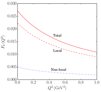
(a)

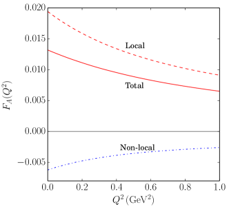
(b)

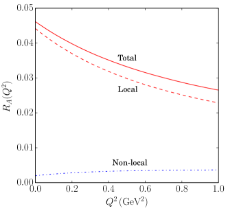
(c)

Figure 2: The form factors $F_{V}(Q^{2})$, $F_{A}(Q^{2})$, and $R_{A}(Q^{2})$ for the radiative pion decay as functions of $Q^{2}$. In the left panel the vector form factor is depicted. The middle and the right panels correspond to the axial-vector form factor and the second axial-vector form factor, respectively. The momentum-dependent quark mass defined in Eq. (13) with Eq. (14) was used. The dashed curve presents the local contribution whereas the dot-dashed one draws the nonlocal contribution. The solid curve depicts the total result.

Figure 2 draws the results of the pion form factors for pion radiative weak decay. In general, the form factors decrease monotonically, as $Q^{2}$ decreases. As discussed in the previous section, it is essential to consider the nonlocal contribution to preserve the corresponding gauge invariances, since the electromagnetic and vector currents should be conserved. As shown in the left panel of Fig. 2, the nonlocal part contributes to the pion vector form factor by almost about 20 %.

The results for the axial-vector form factor is depicted in the middle panel of Fig. 2 as a function of $Q^{2}$. Note that, however, the nonlocal contribution behaves very differently from the case of the vector form factor. In fact, it turns out negative, so that the final result for the form factor is reduced by about 30 %, which implies that it is indeed crucial to consider the nonlocal part in computing the axial-vector form factor. As will be discussed later, it is very important to take into account the nonlocal part to describe the experimental data at $Q^{2}=0$.

The second axial-vector form factor $R_{A}(Q^{2})$ comes into play, when the momentum of the photon is virtual. That is, one can get access to it by $\pi^{+}\to e^{+}\nu_{e}e^{+}e^{-}$ decay in which the virtual photon is annihilated into $e^{+}$ and $e^{-}$. As shown in the right panel of Fig. 2, the $Q^{2}$ dependence of $R_{A}(Q^{2})$ is similar to $F_{A}(Q^{2})$. However, the nonlocal contribution is relatively small and positive. Moreover, it starts to increase as $Q^{2}$ increases, which makes $Q^{2}$ dependence slightly milder than those of the vector and axial-vector form factors. Note that the nonlocal contribution becomes saturated as $Q^{2}$ further increases.

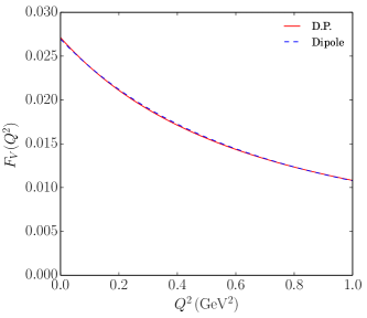
(a)

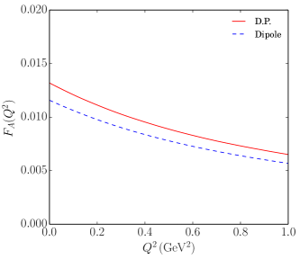
(b)

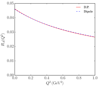
(c)

Figure 3: Comparisons of the form factors, $F_{V}(Q^{2})$, $F_{A}(Q^{2})$ and $R_{A}(Q^{2})$ with two different types of the momentum-dependent quark mass used. The solid curves draw the form factors derived by using the quark mass from the instanton vacuum given in Eq. (14) (D.P.), whereas the dashed ones depict that by the dipole-type mass given in Eq. (15) (Dipole).

In Fig. 3, we compare two different results of the pion weak form factors, employing the two different forms of the dynamical quark mass given in Eq. (14) and Eq. (15), respectively. The dynamical quark mass with the dipole-type parametrization yields almost the same results for the vector and second axial-vector form factors. On the other hand, it gives a smaller result for the axial-vector form factor by around $12\,\%$ in comparison with that from the instanton vacuum.

Table 1: Comparison of the present results with those from other works. “D.P.” stands for the results derive from the instanton vacuum, whereas “Dipole” denotes those obtained from the dipole-type parametrization of the dynamical quark mass.

	NJL Courtoy:2007vy	NL NJL(A) GomezDumm:2012qh	$\chi$PT Unterdorfer:2008zz	Experimental data	Present work
					D.P.	Dipole
$F_{V}(0)$	0.0242	0.0270	0.0262(5)	0.0258(17) Bychkov:2008ws	0.0271	0.0269
$a_{V}$		0.0191	0.0332(42)	0.10(6) Bychkov:2008ws	0.0287	0.0280
$F_{A}(0)$	0.0239	0.0132	0.0106(36)	0.0117(17) Bychkov:2008ws	0.0132	0.0116
$a_{A}$		0.012	0.0191(61)	$-$	0.0192	0.0193
$R_{A}(0)$				$0.059^{+0.009}_{-0.008}$ Egli:1989vu	0.0462	0.0459

In Table 1, we list the results for the form factors at $Q^{2}=0$ and slope parameters that are defined as

$$F_{V}(Q^{2})=\frac{F_{V}(0)}{1+a_{V}\frac{Q^{2}}{m_{\pi}^{2}}},\;\;\;F_{A}(Q^{2})=\frac{F_{A}(0)}{1+a_{A}\frac{Q^{2}}{m_{\pi}^{2}}},$$ (39)

where $a_{V}$ and $a_{A}$ denote the slope parameter for the vector and axial-vector form factors, respectively. The values of the vector and axial-vector form factors at $Q^{2}=0$ are respectively given as $F_{V}(0)=0.0271$, $F_{A}(0)=0.0132$, and $R_{A}(0)=0.0462$ when the dynamical quark mass from the instanton vacuum is used. The dipole-type parametrization yields $F_{V}(0)=0.0269$, $F_{A}(0)=0.0116$, and $R_{A}(0)=0.0459$. As expected from the results for the form factors shown in Fig. 3, the values of $F_{A}(0)$ from these two different forms of the dynamical quark mass are around $12\,\%$ different each other. The results are in good agreement with the experimental data $F_{V}^{\mathrm{exp}}=0.0258(17)$ and $F_{A}^{\mathrm{exp}}=0.0117(17)$ Bychkov:2008ws . It is also of great interest to compare the present results with those from other works. Unterdorfer and Pichl Unterdorfer:2008zz analyzed the vector and axial-vector form factors of pion radiative decay, combining the results from $\chi$PT wirh a large $N_{c}$ expansion and experimental data on other decays. The results are obtained as $F_{V}(0)=0.0262(5)$ and $F_{A}(0)=0.0106(36)$, which are in good agreement with the present results. Courtoy and Noguera Courtoy:2007vy employed the NJL model to study the $\pi$ photo-transition amplitude and derived from it the pion form factors as $F_{V}(0)=0.0242$ and $F_{A}(0)=0.0239$. So, the result of the vector form factor is comparable with that of the present work whereas that of the axial-vector form factor is two times larger than this one.

The results of Ref. GomezDumm:2012qh are especially interesting, since the nonlocal NJL model used in Ref. GomezDumm:2012qh has several aspects in common with the present model. In Ref. GomezDumm:2012qh , three different parameter sets were adopted, among which the results with set A are compared with the present ones. Those from Ref. GomezDumm:2012qh with set A are listed in Table 1 and are in good agreement with the present results except for the slope parameters. It implies that the vector and axial-vector form factors they obtained fall off more slowly than the present ones. What is interesting is that the value $a_{V}=0.032$, which is derived from the empirical fit to $\pi^{0}\to\gamma\gamma^{*}$ experimental data in Ref. GomezDumm:2012qh , is in good agreement with that of the present work.

In $\chi$PT, the values of $F_{A}(0)$ and $R_{A}(0)$ are given in terms of the low-energy constants (LECs), $L_{9}$ and $L_{10}$

$$F_{A}(0)=\frac{4\sqrt{2}m_{\pi}}{f_{\pi}}(L_{9}+L_{10}),\;\;\;R_{A}(0)=\frac{4\sqrt{2}m_{\pi}}{f_{\pi}}L_{9}.$$ (40)

We obtain the values from the present numerical calculation as Table 2.

Table 2: The results of the low-energy constants. “D.P.” stands for the results derive from the instanton vacuum, whereas “Dipole” denotes those obtained from the dipole-type parametrization of the dynamical quark mass.

	$\hskip 14.22636ptL_{9}^{r}$	$\hskip 19.91684ptL_{10}^{r}$	$L_{9}^{r}+L_{10}^{r}$
D.P.	$5.43$	$-3.88$	$1.55$
Dipole	$5.41$	$-4.05$	$1.36$

It is also of interest to extract the parameters for the parametrization of the vector and axial-vector form factors for $\pi$ radiative weak decays. In lattice QCD, the $p$-pole parametrization for a form factor is often utilized Brommel:2006ww ; Brommel:2007xd , which is different from the typical parametrization given in Eq.(39). Then, the present three transition form factors can be parametrized as

$$F_{V}(Q^{2})=\frac{F_{V}(0)}{\left(1+\frac{Q^{2}}{p_{V}m_{p_{V}}^{2}}\right)^{p_{V}}},\;\;\;F_{A}(Q^{2})=\frac{F_{A}(0)}{\left(1+\frac{Q^{2}}{p_{A}m_{p_{A}}^{2}}\right)^{p_{A}}},\;\;\;R_{A}(Q^{2})=\frac{R_{A}(0)}{\left(1+\frac{Q^{2}}{p_{R}m_{p_{R}}^{2}}\right)^{p_{R}}},$$ (41)

where the results of the corresponding parameters are listed in Table 3.

Table 3: The results of the p-pole parameters. “D.P.” stands for the results derive from the instanton vacuum, whereas “Dipole” denotes those obtained from the dipole-type parametrization of the dynamical quark mass.

	$P_{V}$	$M_{P_{V}}$	$P_{A}$	$M_{P_{A}}$	$P_{R}$	$M_{P_{R}}$
D.P.	$1.16$	$0.843$ GeV	$1.48$	$1.05$ GeV	$0.757$	$1.10$ GeV
Dipole	$1.34$	$0.870$ GeV	$1.59$	$1.05$ GeV	$0.734$	$1.12$ GeV

VI Summary and conclusion

In the present work, we aimed at investigating the form factors for pion radiative weak decays, based on the gauged effective chiral action derived from the instanton vaccuum. We computed the vector and axial-vector transition form factors $F_{V}(Q^{2})$, $F_{A}(Q^{2})$, and $R_{A}(Q^{2})$, employing the momentum-dependent dynamical quark mass from the instanton vacuum and that with the dipole-type parametrization. The nonlocal contributions, which arise from the gauging of the effective chiral action, enhance the vector form factor by about $20\,\%$, whereas they reduce the axial-vector form factor $F_{A}(Q^{2})$ by about 30 %. The nonlocal terms influence the second axial-vector form factor marginally. The difference between the results from the instanton vacuum and those with the dipole-type dynamical quark mass is almost the same except for the axial-vector form factor for which the result with the dipole-type parametrization is about $12\,\%$ smaller than that from the instanton vacuum. The present results were compared with the experimental data and were found to be in good agreement with the data except for the slope parameter $a_{V}$. We also derived the low-energy constants $L_{9}^{r}$ and $L_{10}^{r}$. Finally, we parametrized the form factors, using the $p$-pole parametrization, which can be used to compare the present results with those from the lattice data.

It is also of interest to consider other types of the form factors for pion radiative decay such as tensor transition form factors within the present framework. These tensor form factors may give a clue about a right direction beyond the Standard model. Moreover, they will provide an opportunity to understand generalized transition form factors related to the generalized parton distributions for weak processes. Another interesting decay is kaon radiative decay, which will play a role of the touchstone of understanding the effects of flavor SU(3) symmetry in mesonic weak decays. The corresponding works are under way.

References

- (1) V. G. Vaks and B. L. Ioffe, Nuovo Cim. 10 (1958) 342.
- (2) S. A. Bludman and J. A. Young, Phys. Rev. 118 (1960) 602.
- (3) D. A. Bryman, P. Depommier and C. Leroy, Phys. Rept. 88 (1982) 151.
- (4) C. Patrignani et al. (Particle Data Group), Chin. Phys. C. 40 (2016) 100001.
- (5) S. S. Gershtein and Y. B. Zeldovich, Zh. Eksp. Teor. Fiz. 29 (1955) 698.
- (6) P. Depommier, J. Heintze, A. Mukhin, C. Rubbia, V. Soergel and K. Winter, Phys. Lett. 2 (1962) 23.
- (7) P. Depommier, J. Heintze, C. Rubbia and V. Soergel, Phys. Lett. 7 (1963) 285.
- (8) A. Stetz i.e., Nucl. Phys. B 138 (1978) 285.
- (9) A. Bay et al., Phys. Lett. B 174 (1986) 445.
- (10) L. E. Piilonen et al., Phys. Rev. Lett. 57 (1986) 1402.
- (11) S. Egli et al. [SINDRUM Collaboration], Phys. Lett. B 175 (1986) 97.
- (12) S. Egli et al. [SINDRUM Collaboration], Phys. Lett. B 222 (1989) 533.
- (13) V. N. Bolotov et al., Phys. Lett. B 243 (1990) 308.
- (14) E. Frlez et al., Phys. Rev. Lett. 93 (2004) 181804 [hep-ex/0312029].
- (15) M. Bychkov et al., Phys. Rev. Lett. 103 (2009) 051802 [arXiv:0804.1815 [hep-ex]].
- (16) B. R. Holstein, Phys. Rev. D 33 (1986) 3316.
- (17) J. Bijnens and P. Talavera, Nucl. Phys. B 489 (1997) 387 [hep-ph/9610269].
- (18) C. Q. Geng, I. L. Ho and T. H. Wu, Nucl. Phys. B 684 (2004) 281 [hep-ph/0306165]
- (19) V. Mateu and J. Portoles, Eur. Phys. J. C 52 (2007) 325 [arXiv:0706.1039 [hep-ph]].
- (20) R. Unterdorfer and H. Pichl, Eur. Phys. J. C 55 (2008) 273 [arXiv:0801.2482 [hep-ph]].
- (21) N. F. Nasrallah, N. A. Papadopoulos and K. Schilcher, Phys. Lett. 113B (1982) 61.
- (22) D. Gomez Dumm, S. Noguera and N. N. Scoccola, Phys. Lett. B 698 (2011) 236 [arXiv:1011.6403 [hep-ph]]
- (23) D. Gomez Dumm, S. Noguera and N. N. Scoccola, Phys. Rev. D 86 (2012) 074020 [arXiv:1205.2730 [hep-ph]]
- (24) C. H. Chen, C. Q. Geng and C. C. Lih, Phys. Rev. D 83 (2011) 074001 [arXiv:1006.2939 [hep-ph]].
- (25) D. Diakonov and V. Y. Petrov, Nucl. Phys. B 272 (1986) 457.
- (26) D. Diakonov, Prog. Part. Nucl. Phys. 51 (2003) 173 [hep-ph/0212026].
- (27) M. M. Musakhanov and H.-Ch. Kim, Phys. Lett. B 572 (2003) 181 [hep-ph/0206233].
- (28) H.-Ch. Kim, M. Musakhanov and M. Siddikov, Phys. Lett. B 608 (2005) 95 [hep-ph/0411181].
- (29) H.-Ch. Kim, M. M. Musakhanov and M. Siddikov, Phys. Lett. B 633 (2006) 701 [hep-ph/0508211].
- (30) K. Goeke, H.-Ch. Kim, M. M. Musakhanov and M. Siddikov, Phys. Rev. D 76 (2007) 116007 [arXiv:0708.3526 [hep-ph]].
- (31) K. Goeke, M. M. Musakhanov and M. Siddikov, Phys. Rev. D 76 (2007) 076007 [arXiv:0707.1997 [hep-ph]].
- (32) E. V. Shuryak, Nucl. Phys. B 203 (1982) 93.
- (33) T. Schäfer and E. V. Shuryak, Rev. Mod. Phys. 70 (1998) 323 [hep-ph/9610451]
- (34) M. C. Chu, J. M. Grandy, S. Huang and J. W. Negele, Phys. Rev. D 49 (1994) 6039 [hep-lat/9312071].
- (35) J. W. Negele, Nucl. Phys. Proc. Suppl. 73 (1999) 92 [hep-lat/9810053].
- (36) T. A. DeGrand, Phys. Rev. D 64 (2001) 094508 [hep-lat/0106001].
- (37) M. Cristoforetti, P. Faccioli, M. C. Traini and J. W. Negele, Phys. Rev. D 75 (2007) 034008 [hep-ph/0605256].
- (38) M. Musakhanov, Eur. Phys. J. C 9 (1999) 235 [hep-ph/9810295].
- (39) M. Musakhanov, hep-ph/0104163.
- (40) M. Musakhanov, Nucl. Phys. A 699 (2002) 340.
- (41) S. i. Nam and H.-Ch. Kim, Phys. Lett. B 647 (2007) 145 [hep-ph/0605041].
- (42) M. Chretien and R. E. Peierls, Proc. Roy. Soc. Lond. A 223 (1954) 468.
- (43) P. V. Pobylitsa, Phys. Lett. B 226 (1989) 387.
- (44) R. D. Bowler and M. C. Birse, Nucl. Phys. A 582 (1995) 655 [hep-ph/9407336].
- (45) M. M. Musakhanov and F. C. Khanna, hep-ph/9605232.
- (46) S. i. Nam and H.-Ch. Kim, Phys. Rev. D 77 (2008) 094014 [arXiv:0709.1745 [hep-ph]].
- (47) C. G. Callan, Jr., R. F. Dashen and D. J. Gross, Phys. Rev. D 17 (1978) 2717.
- (48) D. Diakonov and V. Y. Petrov, Nucl. Phys. B 245 (1984) 259.
- (49) G. ’t Hooft, Phys. Rev. D 14 (1976) 3432 [Phys. Rev. D 18 (1978) 2199].
- (50) C. W. Bernard, Phys. Rev. D 19 (1979) 3013.
- (51) C. k. Lee and W. A. Bardeen, Nucl. Phys. B 153 (1979) 210.
- (52) S. i. Nam and H.-Ch. Kim, Phys. Rev. D 74 (2006) 076005 [hep-ph/0609267].
- (53) S. i. Nam and H.-Ch. Kim, Phys. Rev. D 75 (2007) 094011 [hep-ph/0703089 [HEP-PH]].
- (54) D. Diakonov, In *Peniscola 1997, Advanced school on non-perturbative quantum field physics* 1-55 [hep-ph/9802298].
- (55) A. Courtoy and S. Noguera, Phys. Rev. D 76 (2007) 094026.
- (56) J. Bijnens and P. Talavera, JHEP 0203 (2002) 046.
- (57) D. Brommel et al. [QCDSF/UKQCD Collaboration], Eur. Phys. J. C 51 (2007) 335 [hep-lat/0608021].
- (58) D. Brommel et al. [QCDSF and UKQCD Collaborations], Phys. Rev. Lett. 101 (2008) 122001 [arXiv:0708.2249 [hep-lat]].