Gaussian autoregressive process with dependent innovations. Some asymptotic results.

Abstract

In this paper we introduce a modified version of a gaussian standard first-order autoregressive process where we allow for a dependence structure between the state variable $Y_{t-1}$ and the next innovation $\xi_{t}$. We call this model dependent innovations gaussian AR(1) process (DIG-AR(1)). We analyze the moment and temporal dependence properties of the new model. After proving that the OLS estimator does not consistently estimate the autoregressive parameter, we introduce an infeasible estimator and we provide its $\sqrt{T}$-asymptotic normality.

Mathematics Subject Classification (2010): 62M10, 62F10

Keywords: autoregressive processes, dependent innovations, $\sqrt{T}$-asymptotic normality.

1 Introduction

In this paper we consider a modified version of the standard first-order autoregressive process, $Y_{t}=\phi Y_{t-1}+\xi_{t}$, in which, unlike the classical case, we assume that the state variable at the time $t-1$, $Y_{t-1}$, and the next innovation $\xi_{t}$ are no longer independent.

The model here considered is a particular case of the class of the C-convolution based processes studied in Cherubini et al. (2011) and Cherubini et al. (2012). Recent literature has mainly focused on stationary copula-based Markov process (see, among the others, Chen and Fan, 2006, and Beare, 2010), while the mentioned C-convolution based processes have a stationary dependence structure between each level and the next innovation generating a process which no longer stationary.

In particular, this paper focuses on the case where the pairs $(Y_{t-1},\xi_{t})_{t}$ have a joint distribution function given by a gaussian copula with a time-invariant parameter $\rho$ and the innovations $(\xi_{t})_{t}$ are identically distributed with a gaussian distribution: in addition, we assume that the resulting stochastic process is a Markov process. This model first appeared in Cherubini et al. (2016) where some moment properties have been analyzed without, however, considering temporal dependencies. The unit root case ($\phi=1$) is studied in Gobbi and Mulinacci (2017) while here we will concentrate on the case $|\phi|<1$. We call the model “dependent innovations gaussian AR(1) process (DIG-AR(1))”.

The analysis of the model starts from the study of the implied temporal dependence properties both in the sequence $(Y_{t})_{t}$ and in the sequence of innovations $(\xi_{t})_{t}$ which, as expected, are no more independent. As a consequence, statistical inference on the model changes significantly. In particular, estimating the autoregressive parameter can no longer be made by ordinary least squares (OLS). As we shall prove, the OLS estimator is not consistent for $\phi$ and, as expected, the asymptotic bias depends on $\rho$. To overcome this drawback, in this paper we propose a new infeasible estimator of $\phi$ which allows us to achieve a $\sqrt{T}$-consistency and asymptotic normality. The new estimator takes into account a correction due to the presence of $\rho$ whose importance will be emphasized both as regards the estimation procedure and as regards the dynamics of the process.

The paper is organized as follows. Section 2 introduces the DIG-AR(1) process. Section 3 shows the autocorrelation functions of $(Y_{t})_{t}$ and $(\xi_{t})_{t}$. In Section 4 we prove that the OLS estimator is not consistent for the autoregressive parameter and we introduce a new infeasible estimator which is proved to be $\sqrt{T}$-asymptotically normal. Section 5 concludes.

2 The model

In this paper we consider a generalized version of the standard stationary gaussian first-order autoregressive process, AR(1), defined as

$$Y_{t}=\phi Y_{t-1}+\xi_{t},$$

where $Y_{0}=0$ a.s., $|\phi|<1$ (condition for the weak stationarity) and the sequence of innovations $(\xi)_{t\geq 1}$ is i.i.d. and normally distributed with zero mean and standard deviation $\sigma_{\xi}$ (gaussian white noise process): as a consequence, $\xi_{t}$ is independent of $Y_{t-1}$ for all $t$. It is just the case to recall that in this framework we have

$$\left\{\begin{array}[]{ll}\mathbb{E}[Y_{t}]=0,\ t\geq 1\\ \mathbb{E}[Y_{t}^{2}]=\frac{\sigma^{2}_{\xi}}{1-\phi^{2}},\ t\geq 1\\ \eta_{k}=corr(Y_{t},Y_{t+k})=\phi^{k},\ k=1,2,...\\ \end{array}\right.$$

For a detailed discussion of AR(1) processes see, among others, Hamilton (1994) and Brockwell and Davis (1991). The modified version of the AR(1) process considered in this paper is inspired by the Markov processes modeling with dependent increments considered in Cherubini et al. (2011, 2012, 2016): the idea is to relax the assumption of independence between $\xi_{t}$ and $Y_{t-1}$, allowing for some time-invariant gaussian dependence.

More precisely

Definition 2.1.

A dependent innovations gaussian AR(1) process (DIG-AR(1)) is a discrete time stochastic process defined as

$$Y_{t}=\phi Y_{t-1}+\xi_{t},\,t\in\mathbb{N}$$ (1)

where $Y_{0}=0$ a.s., $|\phi|<1$, $(\xi_{t})_{t}$ are identically distributed with $\xi_{t}\sim N(0,\sigma^{2}_{\xi})$ and the copula associated to the vector $(\xi_{t},Y_{t-1})$ is gaussian with time-invariant parameter $\rho$ with $|\rho|<1$ for all $t$.

Therefore, in this version of the model the sequence of innovations is no more a gaussian white noise but it has a temporal dependence structure that we will analyze in the following. Moreover, in Section 4.3.1 of Cherubini et al. (2016), the authors determine the variance of $Y_{t}$ and its asymptotic convergence, that is

$$V_{t}^{2}=\sigma_{\xi}^{2}\left(\phi^{2(t-1)}+\sum_{i=1}^{t-1}\phi^{2(i-1)}\right)+2\rho\sigma_{\xi}\sum_{i=1}^{t-1}\phi^{2i-1}V_{t-i},$$

and

$$V_{t}\underset{t\uparrow+\infty}{\longrightarrow}\frac{\sigma_{\xi}\left(\rho\phi+\sqrt{\rho^{2}\phi^{2}+1-\phi^{2}}\right)}{1-\phi^{2}}.$$

The limit, that we denote with $\bar{V}(\rho,\phi)$, can be written as

$$\bar{V}(\rho,\phi)=S\frac{\left(\rho\phi+\sqrt{\rho^{2}\phi^{2}+1-\phi^{2}}\right)}{\sqrt{1-\phi^{2}}},$$

where $S=\frac{\sigma_{\xi}}{\sqrt{1-\phi^{2}}}$ is the standard deviation of the AR(1) process. It is just the case to observe that, when $\rho=0$, $\bar{V}(0,\phi)=S$. As shown in Figure 1, we can notice that $\bar{V}(\rho,\phi)>S$ if $\rho\phi>0$ whereas $\bar{V}(\rho,\phi)<S$ if $\rho\phi<0$. In plain words, $Y_{t}$ becomes more and more volatile if the correlation between $\xi_{t}$ and $Y_{t-1}$ has the same sign of the autoregressive coefficient. On the other hand, the volatility tends to decrease if they have opposite sign.

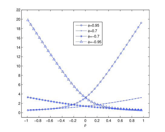
Figure 1: Graph of $\bar{V}(\rho,\phi)$ as a function of $\rho$ for different values of $\phi$. Here we fix $\sigma_{\xi}=1$.

In addition to the above assumptions, we assume that the stochastic process $(Y_{t})_{t}$ is a Markov process. As proved in Darsow et al. (1992) a necessary condition for a process $(Y_{t})_{t}$ to be Markovian is that, if $C_{s,t}$ is the copula associated to $(Y_{s},Y_{t})$, then

$$C_{s,t}(u,v)=C_{s,r}\ast C_{r,t}(u,v)=\int_{0}^{1}\frac{\partial}{\partial w}C_{s,r}(u,w)\frac{\partial}{\partial w}C_{r,t}(w,v)\,dw,\,\forall s<r<t.$$

Morover, as shown in section 3.2.3 in Cherubini et al. (2012), if copulas $C_{s,r}$ and $C_{r,t}$ are gaussian with parameters $\tau_{s,r}$ and $\tau_{r,t}$, respectively, then $C_{s,t}$ is again gaussian with parameter

$$\tau_{s,t}=\tau_{s,r}\tau_{r,t}.$$ (2)

3 Autocorrelation functions and mixing-properties

In this subsection we study the behavior of the autocorrelation functions of the process $(Y_{t})_{t}$ when $t\longrightarrow+\infty$. It is just the case to recall that in the standard AR(1) process the $k$-th order autocorrelation function of $(Y_{t})_{t}$ depends only on $k$ and it is equal to $\phi^{k}$. In our more general setting, this is no longer true. In section 4.3.1 of Cherubini et al. (2016) it is shown that the copula between $Y_{t}$ and $Y_{t+1}$ is gaussian with time-dependent parameter given by

$$\tau_{t,t+1}=\frac{\phi V_{t}+\rho\sigma_{\xi}}{V_{t+1}},$$

and

$$\tau_{t,t+1}\underset{t\uparrow+\infty}{\longrightarrow}\phi+\frac{\rho\sigma_{\xi}}{\bar{V}(\rho,\phi)}=\bar{\tau}(\rho,\phi).$$ (3)

The limit of the $k$-th order autocorrelation function of the Markov process $(Y_{t})_{t}$ is a function of $k$, $\sigma_{\xi}$ and $\rho$ as the following proposition shows.

Proposition 3.1.

The $k$-th order autocorrelation function of the DIG-AR(1) Markov process $(Y_{t})_{t}$ tends to $\left(\phi+\frac{\rho\sigma_{\xi}}{\bar{V}(\rho,\phi)}\right)^{k}$ for any $k\geq 1$ as $t\longrightarrow+\infty$.

Proof.

Thanks to (2), we have that the copula between $Y_{t}$ and $Y_{t+k}$ is gaussian with parameter

$$\tau_{t,t+k}=\prod_{s=0}^{k-1}\frac{\phi V_{t+s}+\rho\sigma_{\xi}}{V_{t+s+1}}.$$

Therefore, since for any $s\geq 1$ as $t\longrightarrow+\infty$

$$\frac{V_{t+s}+\rho\sigma_{\xi}}{V_{t+s+1}}\longrightarrow\frac{\bar{V}(\rho,\phi)+\rho\sigma_{\xi}}{\bar{V}(\rho,\phi)}=\phi+\frac{\rho\sigma_{\xi}}{\bar{V}(\rho,\phi)},$$ (4)

we easily get the result. ∎

It is interesting to consider the role of $\rho$ in the dynamics of the limit of $\tau_{t,t+k}$ with respect to the standard case when $\tau_{t,t+k}=\phi^{k}$. If $\phi>0$ the limit autocorrelation monotonically decreases to zero as $k$ increases, more slowly if $\rho>0$ and more rapidly if $\rho<0$. On the contrary, if $\phi<0$ the limit autocorrelation fluctuates more widely if $\rho<0$ whereas the fluctuations are more blunt if $\rho>0$.

On the other hand, the innovations $(\xi_{t})_{t}$ are of course no longer serially independent as in the standard case and the $k$-th order autocorrelation function approaches to a limit which again depends on $\rho$, $\sigma_{\xi}$ and $k$.

Proposition 3.2.

Given the DIG-AR(1) Markov process of Definition 2.1, the $k$-th order autocorrelation function of $(\xi_{t})_{t}$, $\delta_{t,t+k}$, for any $k\geq 1$, tends to

$$\delta_{t,t+k}\underset{t\uparrow+\infty}{\longrightarrow}\frac{\bar{V}(\rho,\phi)\bar{\tau}^{k-1}(\rho,\phi)}{\sigma_{\xi}^{2}}(\bar{\tau}(\rho,\phi)-\phi)(1-\phi\bar{\tau}(\rho,\phi))$$

where $\bar{\tau}$ is defined in (3).

Proof.

We have

$$\mathbb{E}[\xi_{t}\xi_{t+k}] =\mathbb{E}[(Y_{t}-\phi Y_{t-1})(Y_{t+k}-\phi Y_{t+k-1})]=$$

$$=\mathbb{E}[Y_{t}Y_{t+k}]-\phi\mathbb{E}[Y_{t}Y_{t+k-1}]-\phi\mathbb{E}[Y_{t-1}Y_{t+k}]+\phi^{2}\mathbb{E}[Y_{t-1}Y_{t+k-1}]=$$

$$=\tau_{t,t+k}V_{t}V_{t+k}-\phi\tau_{t,t+k-1}V_{t}V_{t+k-1}-\phi\tau_{t-1,t+k}V_{t-1}V_{t+k}+\phi^{2}\tau_{t-1,t+k-1}V_{t-1}V_{t+k-1}.$$

Since for any fixed $k\geq 1$, $\tau_{t,t+k}\longrightarrow\bar{\tau}^{k-1}(\rho,\phi)$ and $V_{t}\longrightarrow\bar{V}(\rho,\phi)$ as $t\longrightarrow+\infty$ we get

$$\mathbb{E}[\xi_{t}\xi_{t+k}]\longrightarrow \bar{V}^{2}(\rho,\phi)\left(\bar{\tau}^{k}(\rho,\phi)-\phi\bar{\tau}^{k+1}(\rho,\phi)-\phi\bar{\tau}^{k-1}(\rho,\phi)+\phi^{2}\bar{\tau}^{k}(\rho,\phi)\right)=$$

$$=\bar{V}^{2}(\rho,\phi)\bar{\tau}^{k-1}(\rho,\phi)(\bar{\tau}(\rho,\phi)-\phi)(1-\phi\bar{\tau}(\rho,\phi)).$$

It follows

$$\delta_{t,t+k}\longrightarrow\frac{\bar{V}^{2}(\rho,\phi)\bar{\tau}^{k-1}(\rho,\phi)}{\sigma^{2}_{\xi}}(\bar{\tau}(\rho,\phi)-\phi)(1-\phi\bar{\tau}(\rho,\phi)).$$

∎

To conclude this section we briefly discuss the mixing properties of the sequence $(Y_{t})_{t}$. Given a (not necessarily stationary) sequence of random variables $(X_{t})_{t\in\mathbb{Z}}$, defined on a given probability space $(\Omega,\mathcal{F},\mathbb{P})$, let $\mathcal{F}_{t}^{l}$ be the $\sigma$-field $\mathcal{F}_{t}^{l}=\sigma(X_{t},t\leq t\leq l)$ with $-\infty\leq t\leq l\leq+\infty$ and let

$$\tilde{\beta}(\mathcal{F}_{-\infty}^{t},\mathcal{F}_{t+k}^{+\infty})=\sup_{\{A_{i}\},\{B_{j}\}}\frac{1}{2}\sum_{i=1}^{I}\sum_{j=1}^{J}|\mathbb{P}(A_{i}\cap B_{j})-\mathbb{P}(A_{i})\mathbb{P}(B_{j})|,$$ (5)

where the second supremum is taken over all finite partitions $\{A_{1},...A_{I}\}$ and $\{B_{1},...B_{J}\}$ of $\Omega$ such that $A_{i}\in\mathcal{F}_{-\infty}^{t}$ for each $i$ and $B_{j}\in\mathcal{F}_{t+k}^{\infty}$ for each $j$. Define the following dependence coefficient

$$\beta_{k}=\sup_{t\in\mathbb{Z}}\tilde{\beta}(\mathcal{F}_{-\infty}^{t},\mathcal{F}_{t+k}^{+\infty}).$$

We say that the sequence $(X_{t})_{t\in\mathbb{Z}}$ is $\beta-$mixing (or absolutely regular) if $\beta_{k}\rightarrow 0$ as $k\rightarrow+\infty$ (see Volkonskii and Rozanov, 1959 and 1961, for more details).

Proposition 3.3.

The DIG-AR(1) Markov process $(Y_{t})_{t}$ is $\beta$-mixing.

Proof.

The result is an immediate consequence of Theorem 2.1 in Gobbi and Mulinacci (2017) and the proof is very close to that of Corollary 3.1 therein. In fact, since $|\tau_{t,t+1}|<1$ for all $t$ and its limit, $\phi+\frac{\rho\sigma_{\epsilon}}{\bar{V}(\rho,\phi)}$, satisfies $\left|\phi+\frac{\rho\sigma_{\epsilon}}{\bar{V}(\rho,\phi)}\right|<1$, we have that $\hat{\eta}=\underset{t}{\sup}|\tau_{t,t+1}|<1$. Of course, exactly as shown in the proof of Corollary 3.1 of Gobbi and Mulinacci (2017) the density of the copula associated to the vector $(Y_{t},Y_{t+1})$ is uniformly bounded in $L^{2}([0,1])$ and Theorem 2.1 of Gobbi and Mulinacci (2017) applies, allowing to conclude that the process is $\beta$-mixing. ∎

4 An infeasible estimator of the autoregressive parameter

This section is devoted to the analysis of the consistency of the ordinary least squares (OLS) estimator, $\hat{\phi}_{T}$, of the autoregressive coefficient $\phi$ in our DIG-AR(1) markovian model. Unfortunately, unlike the standard case, the OLS estimator is no more consistent. Therefore, we propose an infeasible estimator which is by construction consistent and that it is proved to be $\sqrt{T}$-asymptotically normal.

We recall that given a random sample $(Y_{1},....,Y_{T})$ generated by $(Y_{t})_{t}$, the OLS estimator is $\hat{\phi}_{T}=\frac{\sum_{t=2}^{T}Y_{t}Y_{t-1}}{\sum_{t=2}^{T}Y^{2}_{t-1}}$. In the standard AR(1) model, since $(Y_{t})_{t}$ is a stationary and ergodic process we have that $\hat{\phi}_{T}\stackrel{{\scriptstyle a.s.}}{{\longrightarrow}}\phi$ as $T\longrightarrow+\infty$ (see, among others, Anderson, 1971 and Hamilton, 1994). This is no more the case in our more general context.

Proposition 4.1.

Let $(Y_{t})_{t}$ be a markovian DIG-AR(1) process as in Definition 2.1. Then, the OLS estimator $\hat{\phi}_{T}$ of $\phi$ is not consistent; in particular

$$\hat{\phi}_{T}\stackrel{{\scriptstyle a.s.}}{{\longrightarrow}}\bar{\tau}(\rho,\phi)$$

where $\bar{\tau}(\rho,\phi)$ is defined in (3).

Let’s observe that, coherently with the standard AR(1) process, the OLS estimator converges to the limit of the first-order autocorrelation. Unfortunately, in our DIG-AR(1) model such a first-order autocorrelation does not coincide with the autoregressive parameter.

Proof.

First we observe that the assumption of markovianity of $(Y_{t})_{t}$ implies that, if $(\mathcal{F}_{t})_{t}$ is the filtration generated by $(Y_{t})_{t}$, then $\mathbb{P}(\xi_{t}\leq x|\mathcal{F}_{t-1})=\mathbb{P}(\xi_{t}\leq x|Y_{t-1})$ for all $x\in\mathbb{R}$ and, thanks to the assumptions of the model, the conditional distribution of $\xi_{t}$ given $Y_{t-1}$ is

$$(\xi_{t}|Y_{t-1})\sim N\left(\frac{\rho\sigma_{\xi}}{V_{t-1}}Y_{t-1},\sigma_{\xi}^{2}(1-\rho^{2})\right).$$ (6)

Now, consider the expression of $\hat{\phi}_{T}$,

$$\hat{\phi}_{T}=\frac{\sum_{t=2}^{T}Y_{t}Y_{t-1}}{\sum_{t=2}^{T}Y^{2}_{t-1}}=\phi+\frac{\sum_{t=2}^{T}\xi_{t}Y_{t-1}}{\sum_{t=2}^{T}Y^{2}_{t-1}}.$$

Differently from the standard case (see Andrews, 1988 and Hamilton, 1994) in our setting the ratio $\frac{\sum_{t=2}^{T}\xi_{t}Y_{t-1}}{\sum_{t=2}^{T}Y^{2}_{t-1}}$ does not converge to zero as $T\longrightarrow+\infty$. In particular, the process $(\xi_{t}Y_{t-1})_{t}$ is not a martingale difference sequence and its mean is not constant over time, $\mathbb{E}[\xi_{t}Y_{t-1}]=\rho\sigma_{\xi}V_{t-1}$. However, the process

$$Z_{t}=\xi_{t}Y_{t-1}-Y_{t-1}\mathbb{E}[\xi_{t}|Y_{t-1}]$$ (7)

is a martingale difference sequence with respect to the filtration $(\mathcal{F}_{t})_{t}$ and, since thanks to equation (6), $Y_{t-1}\mathbb{E}[\xi_{t}|Y_{t-1}]=\rho\sigma_{\xi}\frac{Y^{2}_{t-1}}{V_{t-1}}$, we have

$$\hat{\phi}_{T}-\phi=\frac{\sum_{t=2}^{T}Z_{t}}{\sum_{t=2}^{T}Y^{2}_{t-1}}+\rho\sigma_{\xi}\frac{\sum_{t=2}^{T}\frac{Y_{t-1}^{2}}{V_{t-1}}}{\sum_{t=2}^{T}Y^{2}_{t-1}}.$$ (8)

Since, thanks to (6),

$$\mathbb{E}\left[Z_{t}^{2}\right]=\mathbb{E}\left[\mathbb{E}\left[Z_{t}^{2}|Y_{t-1}\right]\right]=\mathbb{E}\left[\sigma_{\xi}^{2}Y_{t-1}^{2}(1-\rho^{2})\right]=\sigma_{\xi}^{2}V^{2}_{t-1}(1-\rho^{2})$$ (9)

and $V_{t}$ is a convergent deterministic sequence and hence bounded by a positive constant $\Delta$, we have that

$$\sup_{t}\mathbb{E}\left[Z_{t}^{2}\right]=\sigma_{\xi}^{2}(1-\rho^{2})\sup_{t}V_{t-1}^{2}\leq\sigma_{\xi}^{2}(1-\rho^{2})\Delta^{2}<+\infty.$$

Since the sequence of the second moments of $Z_{t}$ is bounded, we can apply Theorem 3.77 in White (1984) and conclude that

$$\frac{1}{T}\sum_{t=2}^{T}Z_{t}\stackrel{{\scriptstyle a.s.}}{{\longrightarrow}}0,$$

as $T\longrightarrow+\infty$.

Notice that, since $(Y_{t})_{t}$ is $\beta$-mixing (see Proposition 3.3), also $(Y^{2}_{t})_{t}$ is $\beta$-mixing.
Moreover, (see Bradley, 2007) for a Markov process $(X_{t})_{t}$, (5) can be rewritten as

$$\tilde{\beta}(\mathcal{F}_{-\infty}^{t},\mathcal{F}_{t,t+k}^{+\infty})=\frac{1}{2}\parallel F_{t,t+k}(x,y)-F_{t}(x)F_{t+k}(y)\parallel_{TV}$$

where $\parallel\cdot\parallel_{TV}$ is the total variation norm in the Vitali sense and $F_{t,t+k}$, $F_{t}$ and $F_{t+k}$ are the cumulative distribution functions of $(X_{t},X_{t+k})$, $X_{t}$ and $X_{t+k}$. If $(a_{t})_{t}$ is a sequence of positive constants, it can be easily shown that, as a consequence of the Vitali’s total variation norm definition, the coefficient $\tilde{\beta}(\mathcal{F}_{-\infty}^{t},\mathcal{F}_{t,t+k}^{+\infty})$ calculated for the Markov process $\left(a_{t}X_{t}\right)_{t}$ is exactly the same as that calculated for $(X_{t})_{t}$. This allows to conclude that $\left(\frac{Y^{2}_{t-1}}{V_{t-1}}\right)_{t}$ is $\beta$-mixing.

Since $\sup_{t}\mathbb{E}\left[Y_{t-1}^{4}\right]=3\sup_{t}V_{t-1}^{4}$ and $\sup_{t}\mathbb{E}\left[\frac{Y_{t-1}^{4}}{V_{t-1}}\right]=3\sup_{t}V_{t-1}^{2}$ are both finite, thanks to Theorem 3.57 in White (1984), we have that

$$\frac{1}{T}\sum_{t=2}^{T}Y^{2}_{t-1}-\frac{1}{T}\sum_{t=2}^{T}V^{2}_{t-1}\stackrel{{\scriptstyle a.s.}}{{\longrightarrow}}0$$

and

$$\frac{1}{T}\sum_{t=2}^{T}\frac{Y^{2}_{t-1}}{V_{t-1}}-\frac{1}{T}\sum_{t=2}^{T}V_{t-1}\stackrel{{\scriptstyle a.s.}}{{\longrightarrow}}0.$$

But, thanks to Cesàro averages theorem(see appendix A30 in Billingsley, 1968), we have that $\frac{1}{T}\sum_{t=2}^{T}V^{2}_{t-1}\longrightarrow\bar{V}^{2}(\rho,\phi)$ and $\frac{1}{T}\sum_{t=2}^{T}V_{t-1}\longrightarrow\bar{V}(\rho,\phi)$ and

$$\frac{1}{T}\sum_{t=2}^{T}Y^{2}_{t-1}\stackrel{{\scriptstyle a.s.}}{{\longrightarrow}}\bar{V}^{2}(\rho,\phi)\text{ and }\frac{1}{T}\sum_{t=2}^{T}\frac{Y^{2}_{t-1}}{V_{t-1}}\stackrel{{\scriptstyle a.s.}}{{\longrightarrow}}\bar{V}(\rho,\phi).$$ (10)

Substituting in (8) we get the conclusion.

∎

It is interesting to analyze the impact of the correlation coefficient $\rho$ on the asymptotic bias of the OLS estimator for different and fixed values of the autoregressive parameter $\phi$. In particular, Figure 2 shows the graph of the asymptotic bias $\bar{\tau}(\rho,\phi_{0})-\phi_{0}=\frac{\rho\sigma_{\xi}}{\bar{V}(\rho,\phi_{0})}$: we observe that if $\rho$ and $\phi_{0}$ have the same sign the bias is low and decreases if the value of the autoregressive parameter raises in absolute value; on the other hand, if $\rho$ and $\phi_{0}$ have opposite sign the bias is high and tends to increase with the absolute value of the correlation.

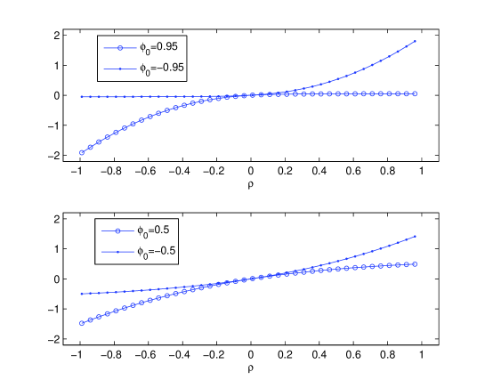
Figure 2: Graph of the asymptotic bias $\bar{\tau}(\rho,\phi_{0})-\phi_{0}=\frac{\rho\sigma_{\xi}}{\bar{V}(\rho,\phi_{0})}$ as a function of $\rho$ for different values of the autoregressive parameter $\phi_{0}$ Here we fix $\sigma_{\xi}=1$.

Thanks to Proposition 4.1 we can introduce a new infeasible estimator $\tilde{\phi}$ of $\phi$, which is consistent by construction, defined as

$$\tilde{\phi}_{T}=\hat{\phi}_{T}-\rho\sigma_{\xi}\frac{\sum_{t=2}^{T}\frac{Y_{t-1}^{2}}{V_{t-1}}}{\sum_{t=2}^{T}Y_{t-1}^{2}}$$ (11)

where $\hat{\phi}$ is the OLS estimator of $\phi$.

The following proposition provides a $\sqrt{T}$-asymptotic normality for $\tilde{\phi}_{T}$.

Theorem 4.1.

Let $(Y_{t})_{t}$ be a markovian DIG-AR(1) process as in Definition 2.1 and $\tilde{\phi}_{T}$ be the infeasible estimator given in (11). Then

$$\sqrt{T}(\tilde{\phi}_{T}-\phi)\stackrel{{\scriptstyle L}}{{\longrightarrow}}X\sim N(0,\bar{\eta}),$$

where $\bar{\eta}=\frac{\sigma_{\xi}\sqrt{1-\rho^{2}}}{\bar{V}(\rho,\phi)}$ and $\stackrel{{\scriptstyle L}}{{\longrightarrow}}$ denotes the convergence in distribution.

Proof.

By (8) we have

$$\sqrt{T}(\tilde{\phi}_{T}-\phi)=\frac{\frac{1}{\sqrt{T}}{\sum_{t=2}^{T}Z_{t}}}{\frac{1}{T}\sum_{t=2}^{T}Y_{t-1}^{2}}.$$ (12)

where $(Z_{t})_{t}$ is the martingale difference defined in (7). Since, see (10), $\frac{1}{T}\sum_{t=2}^{T}Y_{t-1}^{2}\stackrel{{\scriptstyle a.s.}}{{\longrightarrow}}\bar{V}^{2}(\rho,\phi)$, in order to prove the statement, we apply the central limit theorem of Proposition 7.8 in Hamilton (1994) to the numerator in (12). Let us show that the assumptions of that Proposition are satisfied.

Let $\sigma_{t}^{2}=\mathbb{E}\left[Z_{t}^{2}\right]$: thanks to (9) and the assumptions of the model, $\sigma_{t}^{2}>0$ for all $t$ and, using Cesàro averages theorem,

$$\frac{1}{T}\sum_{t=2}^{T}\sigma_{t}^{2}=\sigma_{\xi}^{2}(1-\rho^{2})\frac{1}{T}\sum_{t=2}^{T}V^{2}_{t-1}\longrightarrow\sigma_{\xi}^{2}(1-\rho^{2})\bar{V}^{2}(\rho,\phi)=\bar{\sigma}^{2},$$

which is strictly positive for all $|\rho|<1$ and all $|\phi|<1$. Moreover, it is a straightforward computation to show that $\sup_{t}\mathbb{E}\left[Z_{t}^{4}\right]<+\infty$ and, in order to apply the mentioned central limit theorem, it remains to prove that $\frac{1}{T}\sum_{t=2}^{T}Z_{t}^{2}\stackrel{{\scriptstyle\mathbb{P}}}{{\longrightarrow}}\bar{\sigma}^{2}$.

Since $\mathbb{E}\left[Z_{t}^{2}|Y_{t-1}\right]=\sigma_{\xi}^{2}Y_{t-1}^{2}(1-\rho^{2})$, the process $(W_{t})_{t}$ defined as

$$W_{t}=Z_{t}^{2}-\sigma_{\xi}^{2}Y_{t-1}^{2}(1-\rho^{2})$$

is a martingale difference sequence with respect to the filtration $(\mathcal{F}_{t})_{t}$ generated by the process $(Y_{t})_{t}$. Moreover, since it can be easily shown that $\sup_{t}\mathbb{E}\left[W_{t}^{2}\right]<+\infty$, we can apply Theorem 3.77 in White (1984) to the martingale difference $(W_{t})_{t}$ and conclude that

$$\frac{1}{T}\sum_{t=2}^{T}W_{t}\stackrel{{\scriptstyle a.s.}}{{\longrightarrow}}0.$$

Therefore

$$\frac{1}{T}\sum_{t=2}^{T}Z_{t}^{2}=\frac{1}{T}\sum_{t=2}^{T}W_{t}+\sigma_{\xi}^{2}(1-\rho^{2})\frac{1}{T}\sum_{t=2}^{T}Y_{t-1}^{2}\stackrel{{\scriptstyle a.s.}}{{\longrightarrow}}\bar{\sigma}^{2},$$

as required. Hence, by Proposition 7.8 in Hamilton (1994), we have that $\frac{1}{\sqrt{T}}\sum_{t=2}^{T}Z_{t}$ converges in distribution to a random variable distributed as $N(0,\bar{\sigma})$ and, in conclusion,

$$\sqrt{T}(\tilde{\phi}_{T}-\phi)\stackrel{{\scriptstyle L}}{{\longrightarrow}}X\sim N\left(0,\frac{\sigma_{\xi}\sqrt{1-\rho^{2}}}{\bar{V}(\rho,\phi)}\right),$$

which is the statement of the theorem. ∎

5 Concluding remarks

The paper proposes a modified version of the standard AR(1) process allowing for a time-invariant dependence between the state variable $Y_{t-1}$ and the next innovation $\xi_{t}$. This induces temporal dependence in the sequence of innovations and the standard methods of derivation of the asymptotic properties of the estimators of parameters are no longer applicable. In fact, we show that the standard OLS estimator, generally used for the estimation of the autoregressive parameter, is no more consistent and its asymptotic bias is computed. As a consequence we propose a new infeasible estimator and we establish its $\sqrt{T}$-asymptotic normality.

References

- [1] Anderson T.W. (1971): The Statistical Analysis of Time Series, New York, Wiley.
- [2] Beare B. (2010): ”Copulas and temporal dependence”, Econometrica, 78(1), 395-410.
- [3] Billingsley P. (1968): Convergence of Probability Measures. John Wiley & Sons, New York.
- [4] Bradley R.C. (2007): Introduction to strong mixing conditions, vols. 1-3. Kendrick Press. Herber City.
- [5] Brockwell P. J. - Davis R. A. (1991) Time Series. Theory and Methods, Springer Series in Statistics. Springer-Verlag.
- [6] Chen X., Fan Y. (2006): ”Estimation of Copula-Based Semiparametric Time Series Models”, Journal of Econometrics, 130, 307 335.
- [7] Cherubini U., Gobbi F., Mulinacci S., Romagnoli S. (2012): Dynamic Copula Methods in Finance, John Wiley & Sons.
- [8] Cherubini U., Gobbi F., Mulinacci S., (2016): Convolution Copula Econometrics, SpringerBriefs in Statistics.
- [9] Cherubini, U., Mulinacci S., Romagnoli S. (2011): ”A Copula-based Model of Speculative Price Dynamics in Discrete Time”, Journal of Multivariate Analysis, 102, 1047-1063.
- [10] Darsow W.F. - Nguyen B. - Olsen E.T.(1992): ”Copulas and Markov Processes”, Illinois Journal of Mathematics, 36, 600-642.
- [11] Durante F., Sempi C. (2015): Principles of copula theory, Boca Raton: Chapman and Hall/CRC
- [12] Gobbi F., Mulinacci S. (2017): ”-mixing and moments properties of a non-stationary copula-based Markov process”, http://arxiv.org/abs/1704.01458
- [13] Hamilton J. D. (1994): Time Series Analysis, Princeton University Press.
- [14] Joe H. (1997): Multivariate Models and Dependence Concepts, Chapman & Hall, London
- [15] Nelsen R.(2006): An Introduction to Copulas, Springer
- [16] White H. (1984): Asymptotic theory for econometricians, Academic Press, New York.
- [17] Volkonskii V.A., Rozanov Yu.A. (1959): ”Some limit theorems for random functions I”, Theor. Probab. Appl., 4, 178-197.
- [18] Volkonskii V.A., Rozanov Yu.A. (1961): ”Some limit theorems for random functions II”, Theor. Probab. Appl., 6, 186-198.