Transient Dynamics of Double Quantum Dots Coupled to Two Reservoirs

Abstract

We study the time-dependent properties of double quantum dots coupled to two reservoirs using the nonequilibrium Green function method. For an arbitrary time-dependent bias, we derive an expression for the time-dependent electron density of a dot and several currents, including the current between the dots in the wide-band-limit approximation. For the special case of a constant bias, we calculate the electron density and the currents numerically. As a result, we find that these quantities oscillate and that the number of crests in a single period of the current from a dot changes with the bias voltage. We also obtain an analytical expression for the relaxation time, which expresses how fast the system converges to its steady state. From the expression, we find that the relaxation time becomes constant when the coupling strength between the dots is sufficiently large in comparison with the difference of coupling strength between the dots and the reservoirs.

1 Introduction

Electron transport is a typical example of nonequilibrium phenomena and has been useful for developing the understanding of nonequilibrium statistical physics. Outstanding work on the electron transport was accomplished by Landauer[1] and B$\mathrm{\ddot{u}}$ttiker[2]. They derived a simple formula in which the conductance between leads is expressed in terms of simple physical quantities such as the transmission coefficient. Although the formula was derived for noninteracting electrons with several assumptions, it has been used widely due to its applicability and simplicity. The Landauer-B$\mathrm{\ddot{u}}$ttiker (LB) formula was extended to interacting case in Refs. [3, 4, 5] with the nonequilibrium Green function method[7, 6]. In these studies, the time-dependent current of a system coupled to two leads was expressed in terms of interacting Green functions, even in the case where arbitrary time-dependent biases are applied to leads. For the special case where the system and reservoirs are in a nonequilibrium steady state, the expression for the current reproduces the LB formula.

The approach used in these studies is based on the partitioned approach, which means that a system and reservoirs are in independent equilibrium states characterized by a chemical potential $\mu_{\alpha}$ and an inverse temperature $\beta_{\alpha}$ with $\alpha$ representing the system and the reservoir at an initial time $t_{0}$. After time $t_{0}$, a bias voltage is applied to each reservoir and couplings between the system and the reservoirs are added. When we only consider the steady state, this approach is justified because all effects of the initial condition disappear in the steady state[8]. However, this approach has a problem when we focus on the transient dynamics, where effects of the initial condition cannot be ignored, and in a real experiment we only switch on the bias, not the bias and the coupling. Therefore, the approach is not suitable for investigating the dynamics or time-dependent nonequilibrium properties of nanosystems. The appropriate treatment of this problem may be to set the system and the reservoirs in the same equilibrium state at the initial time, where the couplings between the system and the reservoirs have already been added. This approach is called the partition-free approach. This improvement was introduced in Refs. [9, 8] and applied in Refs. [10, 11, 13, 12]. In the study[10], the authors calculated the Green functions including the effects of the Coulomb interaction with an approximation of the self-energy to conserve physical quantities properly such as energy with the partition-free approach. Without the Coulomb interaction, transport properties were calculated exactly[11] in the wide-band-limit approximation (WBLA). The method of calculation in [11] has been employed to study the case where an arbitrary time-dependent bias is applied to reservoirs[12] and to investigate graphene nanoribbons[13].

Although the authors in the studies above assumed general scatterers and therefore their results are applicable to many systems, we need to consider concrete settings to answer specific questions, such as how the fact that a scatterer consists of several subsystems affects physical quantities. An application of the extended LB formula is the quantum dot. In a quantum dot, many interesting phenomena have been observed such as the Kondo effect[14] due to its low dimensionality. For quantum transport through several quantum dots, one can expect a variety of phenomena to arise from the couplings between the system and the reservoirs or their geometrical configuration. From this viewpoint, many studies on quantum transport through double quantum dots (DQDs) have been conducted experimentally[15, 16, 17, 18] and theoretically[19, 20, 22, 21, 23, 24, 25]. Although there have been many analytical studies of DQDs, the analysis has been mainly carried out in the stationary and special cases. For example, the slave boson approach[19, 20], which has been used widely in the studies of DQDs, assumes that the Coulomb interactions between electrons are very large and that only one electron can exist in each dot. With this approach and the mean-field approximation, many studies on the steady state of DQDs with a parallel, serial, or T-shaped geometry have been made[21, 22, 23, 24]. For the special case where the parameters satisfy the Yang-Baxter relations, the Hamiltonian of DQDs including the Coulomb interaction is exactly solvable with the Bethe ansatz[25]. Understanding the transient dynamics of DQDs themselves is also important for several reasons. One is that DQDs can be applied to quantum computation[26] and studying how the decoherence occurs is important in this context. Moreover, the transient dynamics is interesting as a nonequilibrium phenomenon because of the competition between the initial correlation effects and the existence of coupling between the dots. Until now, theoretical investigations of the transient dynamics of DQDs have mainly been conducted with the master equation[27] or quantum master equation[28], which cannot treat quantum effects such as coherence properly. Some analysis including quantum effect has been conducted numerically[29, 30, 31, 32, 33].

In this paper, to understand the dynamics of DQDs analytically, we study the transient dynamics of DQDs in a serial geometry with the nonequilibrium Green function method and the partition-free approach in the WBLA. We obtain an exact expression for the electron density of a dot and the current between DQDs with arbitrary parameters in the case where the Coulomb interaction is irrelevant. Experimentally, the case in which high bias voltages are applied to reservoirs or the total system is set at a high temperature may be an example of our analysis. For the quenched case, where a constant bias voltage is suddenly applied to a reservoir, we calculate these quantities numerically and clarify the dependence of these quantities on the parameters. From these expressions, we also obtain the relaxation time from any initial condition to the steady state, which is useful for understanding how the decoherence is affected by certain parameters.

The paper is organized as follows. We first introduce the nonequilibrium Green function method in Sect. 2, then we briefly review the previous study of the single dot case[12] in Sect. 3 to highlight the difference between the analysis of the previous case and our case. In Sect. 4, we show the analysis of DQDs, where the second-order partial differential equations for Green functions are derived. We solve the equations and obtain the expressions for the Green functions. We numerically calculate the electron density and the currents in Sect. 5 for the quenched case where a bias voltage is suddenly applied to a reservoir.

2 Nonequilibrium Green Function

The nonequilibrium Green function approach[7, 6] is a method to calculate physical quantities in nonequilibrium many-body quantum systems. It is especially useful for calculating nonequilibrium physical quantities perturbatively. First, we consider a general case and explain the formalism of the nonequilibrium Green function.

We consider the case where there is a central region surrounded by reservoirs. In the central region, there are some subsystems. The total Hamiltonian is represented as $H_{0}$ at initial time $t_{0}$. For the initial state, we assume that the subsystems in the central region and the reservoirs are already coupled and that they are in the same thermal-equilibrium state characterized by an inverse temperature $\beta$ and a chemical potential $\mu$. After the initial time, the perturbative term $V(t)$ is added to the initial Hamiltonian $H(t)=H_{0}+V(t)$. A bias voltage applied to a reservoir is an example of the perturbation. We assume that the total Hamiltonian can be expressed in the matrix form $H(t)=\sum_{ij}h_{ij}(t)d^{\dagger}_{i}d_{j}$. The operators $d^{\dagger}_{i},d_{i}$ express the creation and annihilation operators of the system or the reservoirs.

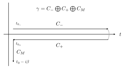
Fig. 1: (Color Online) Konstantinov-Perel’ contour $\gamma$.

Here, we define the Konstantinov-Perel’ contour $\gamma$, which is an extension of the Keldysh contour to include the effects of the initial state, as shown in Fig. 1. The contour consists of three paths: $C_{-}:\{t_{0}\rightarrow\infty\},C_{+}:\{\infty\rightarrow t_{0}\}$ and, $C_{M}:\{t_{0}\rightarrow t_{0}-i\beta\}$. The nonequilibrium Green function on the contour is defined as

$$G_{ij}(z_{1},z_{2}):=-i\frac{1}{Z}\mathrm{Tr}[e^{-\beta H_{0}}\mathcal{T}_{c}[d_{i}(z_{1})d^{\dagger}_{j}(z_{2})]],$$ (1)

where $Z=\mathrm{Tr}e^{-\beta H_{0}}$ is the partition function at the initial time. Here $z=t_{-},t_{+},t_{0}-i\tau$ represents a position on the contour and the time. $t_{-}$ and $t_{+}$ express time $t$ on the paths $C_{-}$ and $C_{+}$ respectively. $\tau(0<\tau<\beta)$ is an imaginary time on path $C_{M}$. The operators appearing in Eq. (1) are defined as

$$d_{i}(z):=\begin{cases}d_{H,i}(t),&z\in C_{-}\bigoplus C_{+},\\ d^{M}_{i}(\tau),&z\in C_{M},\end{cases}$$

where $d_{H,i}(t):=e^{i\int^{t}_{t_{0}}dsH(s)}de^{-i\int^{t}_{t_{0}}dsH(s)}$ is the operator in the Heisenberg picture and $d^{M}(\tau)$ is the Matsubara operator $d^{M}(\tau):=e^{H_{0}\tau}de^{-H_{0}\tau}$. $\mathcal{T}_{c}$ is the contour-ordering operator which depends on the direction of the arrow on the contour. The nonequilibrium Green function Eq. (1) takes several forms according to the positions of the two arguments $z_{1}$ and $z_{2}$. We represent these Green functions in Table I.

Symbol	Position on the contour $\gamma$	Name
$G^{--}_{ij}(t_{1},t_{2})$	$z_{1},z_{2}\in C_{-}$
$G^{++}_{ij}(t_{1},t_{2})$	$z_{1},z_{2}\in C_{+}$
$G^{>}_{ij}(t_{1},t_{2})$	$(z_{1}>z_{2})\land(z_{1},z_{2}\in C_{-}\bigoplus C_{+})$	Greater
$G^{<}_{ij}(t_{1},t_{2})$	$(z_{1}<z_{2})\land(z_{1},z_{2}\in C_{-}\bigoplus C_{+})$	Lesser
$G^{\rceil}_{ij}(t_{1},\tau_{2})$	$(z_{1}\in C_{-}\bigoplus C_{+})\land(z_{2}\in C_{M})$	Right
$G^{\lceil}_{ij}(\tau_{1},t_{2})$	$(z_{1}\in C_{M})\land(z_{2}\in C_{-}\bigoplus C_{+})$	Left
$G^{M}_{ij}(\tau_{1},\tau_{2})$	$z_{1},z_{2}\in C_{M}$	Matsubara

Table 1: Definitions of the Green functions.

As an example, let us consider the case where these two arguments appearing in the Eq. (1) are in part of the contour $z_{1},z_{2}\in C_{-}\bigoplus C_{+}$ and $z_{1}$ is in front of $z_{2}$ on the contour. In this case, since the argument $z_{1}$ is always in front of $z_{2}$, $\mathcal{T}_{c}$ exchanges these two operators and then $(-1)$ is multiplied. Therefore, the nonequilibrium Green function takes the form $G^{<}_{ij}(t_{1},t_{2})=i/Z\mathrm{Tr}[e^{-\beta H_{0}}d_{H,i}^{\dagger}(t_{2})d_{H,j}(t_{1})]$ for $(z_{1}<z_{2})\land(z_{1},z_{2}\in C_{-}\bigoplus C_{+})$. This function is called the lesser Green function. We also define retarded/advanced Green functions as

$$G_{ij}^{r}(t_{1},t_{2}) := \theta(t_{1}-t_{2})[G^{>}_{ij}(t_{1},t_{2})-G^{<}_{ij}(t_{1},t_{2})],$$ (2)

$$G_{ij}^{a}(t_{1},t_{2}) := -\theta(t_{2}-t_{1})[G^{>}_{ij}(t_{1},t_{2})-G^{<}_{ij}(t_{1},t_{2})],$$ (3)

where $\theta(t)$ is the Heaviside function $\theta(t)=1(t>0),0(t<0)$.

We define the Hamiltonian on the contour $h_{ij}(z)$ as

$$h_{ij}(z):=\begin{cases}h_{ij}(t),&z\in C_{-}\bigoplus C_{+},\\ h_{ij}(t_{0}),&z\in C_{M}.\end{cases}$$

Using the contour $\gamma$ and the nonequilibrium Green function on the contour, we can use the diagram technique even in the nonequilibrium case. For details, see [34].

3 Single-Dot Case

Before we discuss the DQD case, which is our main interest, we briefly review the case of a single dot that has only one energy level and is coupled to two reservoirs. This is a special case of [12]. In this case, we analyze the equation of motion for the nonequilibrium Green function. The equation is self-consistent but it becomes solvable after employing the WBLA. By solving the equation of motion, we can obtain a closed-form expression for the nonequilibrium Green function. This section will be useful for understanding the differences between the analysis of the single-dot case and that of the double-dots case, where we cannot obtain a closed-form expression for the nonequilibrium Green function by solving the equation of motion with the WBLA.

3.1 Definition of system

We consider the case where the total system consists of a quantum dot in the central region and two reservoirs. At an initial time $t_{0}$, the dot and the reservoirs are in the thermal-equilibrium state characterized by an inverse temperature $\beta$ and a chemical potential $\mu$. After the time $t\geq t_{0}$, a bias voltage $V_{\alpha}(t)$ is applied to reservoir $\alpha$ and then the total system tends to a nonequilibrium state. The Hamiltonian of the total system is represented as

$$H(t)=\sum_{k\alpha}\epsilon_{k\alpha}(t)d^{\dagger}_{k\alpha}d_{k\alpha}+\epsilon_{1}(t)d^{\dagger}_{1}d_{1}+V,$$ (4)

where $\epsilon_{k\alpha}(t)$ and $\epsilon_{1}(t)$ are defined as $\epsilon_{k\alpha}(t)=\epsilon_{k\alpha}-\mu(t<t_{0}),\epsilon_{k\alpha}+V_{\alpha}(t)(t\geq t_{0})$ and $\epsilon_{1}(t)=\epsilon_{1}-\mu(t<t_{0}),\epsilon_{1}(t\geq t_{0})$. $\epsilon_{k\alpha}$ is the $k$th eigenvalue of the Hamiltonian of reservoir $\alpha$ and $\epsilon_{1}$ is the eigenvalue of the dot. $d_{k\alpha},d^{\dagger}_{k\alpha}$ are the creation and the annihilation operators of reservoir $\alpha$ and $d_{1},d^{\dagger}_{1}$ are those of the dot, respectively. In this case, the particles are fermions and thus these operators satisfy the anticommutation relations $\{d_{i},d^{\dagger}_{j}\}=\delta_{ij},$ $\{d_{i},d_{j}\}=\{d^{\dagger}_{i},d^{\dagger}_{j}\}=0$, where the index $i$ denotes the index of a reservoir $\alpha$ or the dot $i=k\alpha,1$. Each term of the total Hamiltonian has the following meaning: the first term is the (diagonalized) Hamiltonian of the reservoirs, the second is the Hamiltonian of the dot, and the third is the coupling between the dot and the reservoirs. We assume that the coupling term takes the form

$$V=\sum_{k\alpha}T_{k\alpha,1}d^{\dagger}_{k\alpha}d_{1}+T_{1,k\alpha}d^{\dagger}_{1}d_{k\alpha}.$$

We use a matrix representation of the Hamiltonian $h_{ij}(t)$ of the total system to match Ex. (4). For example, when the indices are $i=k\alpha$ and $j=k^{\prime}\alpha$, the value of $h_{ij}(t)$ is

$$h_{k\alpha,k^{\prime}\alpha}(t)=\begin{cases}(\epsilon_{k\alpha}-\mu)\delta_{k,k^{\prime}},&t<t_{0},\\ (\epsilon_{k\alpha}+V_{\alpha}(t))\delta_{k,k^{\prime}},&t\geq t_{0}.\end{cases}$$

We define the matrix $\mathbf{h}_{\alpha\alpha}(t)$ by $[\mathbf{h}_{\alpha\alpha}(t)]_{k,k^{\prime}}=h_{k\alpha,k^{\prime}\alpha}(t)$. Similarly, we define other matrices $\mathbf{h}_{\alpha\alpha}(t),\mathbf{h}_{\alpha 1},\mathbf{h}_{1\alpha}$, and $h_{11}(t)$.

3.2 Equations of motion and previous result

By differentiating the definition of each Green function and using the commutation relations, we derive the equations of motion for the nonequilibrium Green functions as

$$\left[i\frac{d}{dz_{1}}-h_{11}(z_{1})\right]G_{11}(z_{1},z_{2})=\delta(z_{1},z_{2})+\sum_{\alpha}\mathbf{h}_{1\alpha}\mathbf{G}_{\alpha 1}(z_{1},z_{2}),$$ (5)

$$G_{11}(z_{1},z_{2})\left[-i\frac{\overleftarrow{d}}{dz_{2}}-h_{11}(z_{2})\right]=\delta(z_{1},z_{2})+\sum_{\alpha}\mathbf{G}_{1\alpha}(z_{1},z_{2})\mathbf{h}_{\alpha 1},$$ (6)

$$\left[i\frac{d}{dz_{1}}-\mathbf{h}_{\alpha\alpha}(z_{1})\right]\mathbf{G}_{\alpha 1}(z_{1},z_{2})=\mathbf{h}_{\alpha 1}G_{11}(z_{1},z_{2}),$$ (7)

$$\mathbf{G}_{1\alpha}(z_{1},z_{2})\left[-i\frac{\overleftarrow{d}}{dz_{2}}-\mathbf{h}_{\alpha\alpha}(z_{2})\right]=G_{11}(z_{1},z_{2})\mathbf{h}_{1\alpha},$$ (8)

where we use the matrix representation of the nonequilibrium Green function $[\mathbf{G}(z_{1},z_{2})]_{ij}=G_{ij}(z_{1},z_{2})$. The nonequilibirum Green function is defined in the same way as Eq. (1). The operator $\frac{\overleftarrow{d}}{dz}$ is the differential operator acting from the right side.

We need an expression for the lesser Green function to obtain an expression for one-particle quantities such as the electron density of the dot. To obtain an expression for the lesser Green function, we need to solve the equations of motion with the Kubo-Martin-Schwinger(KMS) boundary conditions[35, 36]. All Green functions must satisfy the KMS conditions, which arise from the condition that the initial state is in thermal equilibrium. The KMS conditions are expressed as

$$\begin{cases}\mathbf{G}(z_{1},t_{0}-i\beta)=-\mathbf{G}(z_{1},t_{0}),\\ \mathbf{G}(t_{0}-i\beta,z_{2})=-\mathbf{G}(t_{0},z_{2}),\end{cases}$$ (9)

which are directly derived from definition (1). Note that we can choose another initial condition, as in the partitioned approach, where the system and the reservoirs are in different equilibrium states at the initial time. However this sometime leads to unphysical behavior of physical quantities[8]. Since there are unknown functions in the equations of motion for $G_{11}(z_{1},z_{2})$, (5) and (6), we cannot obtain a closed-form expression for $G_{11}(z_{1},z_{2})$. Now we express the solutions of Eqs. (7) and (8) as

$$\mathbf{G}_{\alpha 1}(z_{1},z_{2}) = \int_{\gamma}d\bar{z}\mathbf{g}_{\alpha\alpha}(z_{1},\bar{z})\mathbf{h}_{\alpha 1}(\bar{z})G_{11}(\bar{z},z_{2}),$$ (10)

$$\mathbf{G}_{1\alpha}(z_{1},z_{2}) = \int_{\gamma}d\bar{z}G_{11}(z_{1},\bar{z})\mathbf{h}_{1\alpha}(\bar{z})\mathbf{g}_{\alpha\alpha}(\bar{z},z_{2}),$$ (11)

where $\mathbf{g}_{\alpha\alpha}$ is the non-perturbative Green function of reservoir $\alpha$, which obeys the equation of motion

$$\left[i\frac{d}{dz_{1}}-\mathbf{h}_{\alpha\alpha}(z_{1})\right]\mathbf{g}_{\alpha\alpha}(z_{1},z_{2})=\mathbf{1}\delta(z_{1},z_{2}),$$

and $\int_{\gamma}d\bar{z}$ is the integration on contour $\gamma$. This equation of motion is equal to that for the isolated reservoir $\alpha$ since there is only the delta function in the right-hand-side(RHS) of the equation. Actually, we can check that expressions (10) and (11) are solutions of the equations of motion (7) and (8) satisfying the KMS conditions. Then, by substituting Eqs. (10) and (11) into Eqs. (5) and (6), finally we obtain the equation of motion for $G_{11}(z_{1},z_{2})$,

$$\begin{split}\left[i\frac{d}{dz_{1}}-h_{11}(z_{1})\right]G_{11}(z_{1},z_{2})&=\delta(z_{1},z_{2})+\int_{\gamma}d\bar{z}\Sigma_{11}(z_{1},\bar{z})G_{11}(\bar{z},z_{2}),\\ G_{11}(z_{1},z_{2})\left[-i\frac{\overleftarrow{d}}{dz_{2}}-h_{11}(z_{2})\right]&=\delta(z_{1},z_{2})+\int_{\gamma}d\bar{z}G_{11}(z_{1},\bar{z})\Sigma_{11}(\bar{z},z_{2})\end{split}$$ (12)

where $\Sigma_{11}$ is the embedded self-energy defined as

$$\Sigma_{11}(z_{1},z_{2})=\mathbf{h}_{1\alpha}(z_{1})\mathbf{g}_{\alpha\alpha}(z_{1},z_{2})\mathbf{h}_{\alpha 1}(z_{2}).$$ (13)

At this point, we obtain a closed-form expression for the embedded self-energy because it is expressed in terms of the known parameters and the non-perturbative Green function, which is calculated easily. Now we use the WBLA. This approximation means that the energy bands of reservoirs are very wide and that only the electrons on the Fermi energy are transported. Mathematically, the WBLA is equivalent to the substitution $\sum_{k}\rightarrow\int\frac{dk}{2\pi}\rightarrow\rho(\epsilon_{F})\int d\epsilon_{k}$, where $\rho_{\epsilon_{F}}$ is the density of states in the vicinity of the Fermi energy. Therefore, the level width $\Gamma_{\alpha}(\omega)=2\pi\sum_{k}T_{1,k\alpha}T_{k\alpha,1}\delta(\omega-\epsilon_{k\alpha})$ becomes a constant $\Gamma_{\alpha}$ and the embedded self-energy takes a simple form in this approximation. For example, the retarded self-energy $\Sigma^{r}_{11}(t_{1},t_{2}):=\theta(t_{1}-t_{2})(\Sigma^{>}_{11}(t_{1},t_{2})-\Sigma^{<}_{11}(t_{1},t_{2}))$ in the WBLA is written as

$$\Sigma^{r}_{11}(t_{1},t_{2})=-\frac{i}{2}\Gamma\delta(t_{1}-t_{2}),$$

where $\Gamma=\sum_{\alpha}\Gamma_{\alpha}$ is the total level width. The lesser $\Sigma^{<}_{11}(t_{1},t_{2})$ and greater $\Sigma^{>}_{11}(t_{1},t_{2})$ self-energies are defined similarly to the lesser and greater Green functions in Sect. 2, respectively. For the derivation, see Appendix A. The calculation of the self-energy in Appendix A is for the case of the DQDs, but the self-energy for the single-dot case is obtained in the same way.

From the equation of motion (12) and the embedded self-energy in the WBLA, we can obtain the following equations of motion for the Matsubara, right/left, and lesser Green functions in the WBLA:

$$\left[-\frac{d}{d\tau_{1}}-h^{M}_{11}\right]G^{M}_{11}(\tau_{1},\tau_{2})=i\delta(\tau_{1}-\tau_{2})+\left(\Sigma^{M}_{11}*G^{M}_{11}\right)_{(\tau_{1},\tau_{2})},$$ (14)

$$\begin{split}\left(i\frac{d}{dt_{1}}-h^{eff}_{11}\right)G^{\rceil}_{11}(t_{1},\tau_{2})&=\left(\Sigma^{\rceil}_{11}*G^{M}_{11}\right)_{(t_{1},\tau_{2})},\\ G^{\lceil}_{11}(\tau_{1},t_{2})\left(-i\frac{\overleftarrow{d}}{dt_{2}}-h^{eff}_{11}\right)&=\left(G^{M}_{11}*\Sigma^{\lceil}_{11}\right)_{(\tau_{1},t_{2})},\end{split}$$ (15)

$$\left(i\frac{d}{dt_{1}}-h^{eff}_{11}\right)G^{<}_{11}(t_{1},t_{2})=\left(\Sigma^{<}_{11}\cdot G^{a}_{11}+\Sigma^{\rceil}_{11}*G^{\lceil}_{11}\right)_{(t_{1},t_{2})},$$ (16)

where $h^{M}_{11}$ is the energy on the vertical part of the contour $\gamma$ and $h^{eff}_{11}$ is the effective energy of the system: $h^{M}_{11}=\epsilon_{1}-\mu$,  $h^{eff}_{11}:=h_{11}-i\Gamma/2$. $(f\cdot g)_{(t,t^{\prime})}$ is the convolution of $f$ and $g$ and $(f*g)_{(\tau,\tau^{\prime})}$ is the imaginary time convolution of $f$ and $g$: $(f\cdot g)_{(t,t^{\prime})}=-i\int^{\infty}_{t_{0}}dsf(t,s)g(s,t^{\prime})$, $(f*g)_{(\tau,\tau^{\prime})}=\int^{\beta}_{0}dsf(\tau,s)g(s,\tau^{\prime})$. In this derivation, we use the Langreth rule[37] to convert the integration in the most RHS of (12) to an integral along the real axis. Since we have an expression of the Matsubara self-energy, we can obtain an expression of the Matsubara Green function from Eq. (14) by applying the Fourier transformation. Then, the resulting equations are inhomogeneous first-order differential equations and thus we can solve these equations. Details of these calculations are given in [12]. Finally, we obtain the following expression of the lesser Green function:

$$G^{<}_{11}(t_{1},t_{2})=e^{-ih^{eff}_{11}(t_{1}-t_{0})}\int^{\infty}_{-\infty}d\omega f(\omega-\mu)\sum_{\alpha}[K_{\alpha}(t_{1},t_{0};\omega)\Gamma_{\alpha}G^{a}(\omega)-G^{r}(\omega)\Gamma_{\alpha}K^{*}_{\alpha}(t_{2},t_{0};\omega)\\ +iK_{\alpha}(t_{1},t_{0};\omega)\Gamma_{\alpha}K^{*}_{\alpha}(t_{2},t_{0};\omega)+iA_{\alpha}(\omega)]e^{i(h^{eff}_{11})^{*}(t_{2}-t_{0})},$$ (17)

where $G^{r}(\omega)=\{\omega-h^{eff}_{11}\}^{-1}$ and $G^{a}(\omega)=\{\omega-(h^{eff}_{11})^{*}\}^{-1}$ are Fourier transforms of the retarded/advanced Green functions, respectively. $f(\omega)=\left\{e^{\beta\omega}+1\right\}^{-1}$ is the Fermi distribution function. Here, we introduce the spectral function $A_{\alpha}(\omega)=G^{r}(\omega)\Gamma_{\alpha}G^{a}(\omega)$ and the function

$$K_{\alpha}(t,t_{0};\omega)=\int^{t}_{t_{0}}dse^{-i(\omega-h^{eff}_{11})(s-t_{0})}e^{-i\psi_{\alpha}(s,t_{0})},$$

which includes all the effects from the biased voltage $\psi_{\alpha}(t,t_{0}):=\int^{t}_{t_{0}}dsV_{\alpha}(s)$. Since the electron density is expressed as $\rho(t)=-iG^{<}_{11}(t,t)$, we calculate the electron density almost directly. Using the concrete expression (17), we calculate the electron density numerically for the quenched case where a constant bias voltage is applied suddenly: $V_{L}=6,V_{R}=0$. We take other parameters as $\epsilon_{1}=1,\Gamma_{L}=\Gamma_{R}=1/2$, and $\beta=100$.

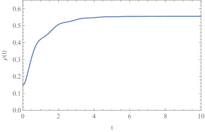
Fig. 2: (Color Online) Time dependence of electron density $\rho$ for $\beta=100$.

We can see that the electron density approaches the limiting value exponentially without oscillation (Fig. 2). This is because we consider a dot having only one energy level. When we consider the case of double dots, however, an oscillation appears even though each dot has only one energy level. See Fig. 4 in Sect. 5 for this argument.

4 Double-Dot Case

4.1 Definition of system

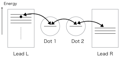
Fig. 3: (Color Online) Schematic diagram of system and reservoirs.

Next, we consider the case of the DQDs, which is the main target of our study. Figure 3 is a schematic diagram of this case. In the case, there are two quantum dots, not one, in the central region. Since there is coupling between the dots, we can expect that richer phenomena will arise than those of the single dot. We assume that the initial condition is the same as in the case of the single dot in Sect. 4. At an initial time $t_{0}$, the dots and the reservoirs are in the thermal-equilibrium state characterized by an inverse temperature $\beta$ and a chemical potential $\mu$. After the initial time $t\geq t_{0}$, a bias voltage $V_{\alpha}(t)$ is applied to each reservoir $\alpha$ and the system enters a nonequilibrium state. The Hamiltonian of the total system is represented as

$$H(t)=\\ \begin{cases}\sum_{\alpha=\{L,R\},k\alpha}(\epsilon_{k\alpha}-\mu)d^{\dagger}_{k\alpha}d_{k\alpha}+\sum_{n=\{1,2\}}(\epsilon_{n}-\mu)d^{\dagger}_{n}d_{n}+V_{1L}+V_{2R}+T_{d},&t<t_{0}\\ \sum_{\alpha=\{L,R\},k\alpha}(\epsilon_{k\alpha}+V_{\alpha}(t))d^{\dagger}_{k\alpha}d_{k\alpha}+\sum_{n=\{1,2\}}\epsilon_{n}d^{\dagger}_{n}d_{n}+V_{1L}+V_{2R}+T_{d},&t\geq t_{0}\end{cases}$$ (18)

where $\epsilon_{k\alpha}$ is the $k$th eigenvalue of the Hamiltonian of reservoir $\alpha$ and $\epsilon_{n}$ is the eigenvalue of dot $n$ $(n=1,2)$. We assume that the Hamiltonian of the reservoirs can be diagonalized and that each dot has just one energy level. $d_{k\alpha},d^{\dagger}_{k\alpha}$ are the creation and annihilation operators of reservoir $\alpha$ and $d_{n},d^{\dagger}_{n}$ are those of dot $n$, respectively. The transported particles are fermions and thus the operators satisfy the anticommutation relations $\{d_{i},d^{\dagger}_{j}\}=\delta_{ij}$, $\{d_{i},d_{j}\}=\{d^{\dagger}_{i},d^{\dagger}_{j}\}=0$. Each term of the Hamiltonian has the following meaning: the first term is the (diagonalized) Hamiltonian of the reservoirs, the second is the Hamiltonian of the dots, the third is the coupling between dot 1 and the left reservoir, the fourth is the coupling between dot 2 and the right reservoir and, the fifth, which does not appear in the case of a single dot, is the coupling between the two dots. Here, we assume that the interactions are written in the forms

$$V_{i\alpha} = \sum_{k\alpha,n}T_{k\alpha,n}d^{\dagger}_{k\alpha}d_{n}+T_{n,k\alpha}d^{\dagger}_{n}d_{k\alpha},$$

$$T_{d} = t_{12}d^{\dagger}_{1}d_{2}+t_{21}d^{\dagger}_{2}d_{1}.$$

Note that we are interested in how the fact that the central system consists of two subsystems affects physical quantities. For this reason, we consider the region where the Coulomb interaction can be ignored. If there was an effect of the Coulomb interaction, there would be more interesting phenomena, but it would be difficult to tell whether the cause of a phenomenon is from the fact that the system consists of some subsystems or from the Coulomb interaction. Experimentally, this approximation may be justified when the energy scale of electrons is larger than that of the Coulomb interaction, i.e., when a high bias voltage is applied or when a system is at a high temperature. We represent the Hamiltonian of the total system (18) in the same way as in the single-dot case,

$$H(t)=\sum_{ij}h_{ij}(t)d^{\dagger}_{i}d_{j},$$

where index $i$ can be $k\alpha$ or $n$ and the elements of $h_{ij}(t)$ are defined to match Eq. (18). We also define the contour $\gamma$ and the nonequilibrium Green function in the same way as in Sect. 3.

4.2 Equation of motion for nonequilibrium Green function

By differentiating the definition of each Green function in Table I and using the anticommutation relations for fermions, we can derive following equations of motion for the nonequilibrium Green functions:

$$\left[i\frac{d}{dz_{1}}-h_{11}(z_{1})\right]G_{11}(z_{1},z_{2})=\delta(z_{1},z_{2})+\mathbf{h}_{1L}\cdot\mathbf{G}_{L1}(z_{1},z_{2})+t_{12}G_{21}(z_{1},z_{2}),$$ (19)

$$G_{11}(z_{1},z_{2})\left[-i\frac{\overleftarrow{d}}{dz_{2}}-h_{11}(z_{2})\right]=\delta(z_{1},z_{2})+\mathbf{G}_{1L}(z_{1},z_{2})\cdot\mathbf{h}_{L1}+G_{12}(z_{1},z_{2})t_{21},$$ (20)

$$\left[i\frac{d}{dz_{2}}-h_{22}(z_{1})\right]G_{22}(z_{1},z_{2})=\delta(z_{1},z_{2})+\mathbf{h}_{2R}\cdot\mathbf{G}_{R2}(z_{1},z_{2})+t_{21}G_{12}(z_{1},z_{2}),$$ (21)

$$G_{22}(z_{1},z_{2})\left[-i\frac{\overleftarrow{d}}{dz_{2}}-h_{22}(z_{2})\right]=\delta(z_{1},z_{2})+\mathbf{G}_{2R}(z_{1},z_{2})\cdot\mathbf{h}_{R2}+G_{21}(z_{1},z_{2})t_{12}.$$ (22)

In the case of double dots, we must consider the equations of motion for not only $G_{11}$ and $G_{22}$ but also $G_{12}$ and $G_{21}$ for analysis:

$$\left[i\frac{d}{dz_{1}}-h_{11}(z_{1})\right]G_{12}(z_{1},z_{2})=\mathbf{h}_{1L}\cdot\mathbf{G}_{L2}(z_{1},z_{2})+t_{12}G_{22}(z_{1},z_{2}),$$ (23)

$$G_{12}(z_{1},z_{2})\left[-i\frac{\overleftarrow{d}}{dz_{2}}-h_{22}(z_{2})\right]=\mathbf{G}_{1R}(z_{1},z_{2})\cdot\mathbf{h}_{R2}+G_{11}(z_{1},z_{2})t_{12},$$ (24)

$$\left[i\frac{d}{dz_{1}}-h_{22}(z_{1})\right]G_{21}(z_{1},z_{2})=\mathbf{h}_{2R}\cdot\mathbf{G}_{R1}(z_{1},z_{2})+t_{21}G_{11}(z_{1},z_{2}),$$ (25)

$$G_{21}(z_{1},z_{2})\left[-i\frac{\overleftarrow{d}}{dz_{2}}-h_{11}(z_{2})\right]=\mathbf{G}_{2L}(z_{1},z_{2})\cdot\mathbf{h}_{L1}+G_{22}(z_{1},z_{2})t_{21},$$ (26)

$$\left[i\frac{d}{dz_{1}}-\mathbf{h}_{LL}(z_{1})\right]\mathbf{G}_{L1}(z_{1},z_{2})=\mathbf{h}_{L1}G_{11}(z_{1},z_{2}),$$ (27)

$$\left[i\frac{d}{dz_{1}}-\mathbf{h}_{RR}(z_{1})\right]\mathbf{G}_{R1}(z_{1},z_{2})=\mathbf{h}_{R2}G_{21}(z_{1},z_{2}),$$ (28)

where we use the matrix representation of the nonequilibrium Green function $\{\mathbf{G}(z_{1},z_{2})\}_{ij}=G_{ij}(z_{1},z_{2})$. As in the case of the single dot in Sect. 3, all Green functions must satisfy the KMS conditions

$$\begin{cases}\mathbf{G}(z_{1},t_{0}-i\beta)=-\mathbf{G}(z_{1},t_{0}),\\ \mathbf{G}(t_{0}-i\beta,z_{2})=-\mathbf{G}(t_{0},z_{2}).\end{cases}$$ (29)

We can construct solutions of equations (27) and (28) satisfying the KMS conditions in the form

$$\mathbf{G}_{L1} = \int_{\gamma}d\bar{z}\mathbf{g}_{LL}(z_{1},\bar{z})\mathbf{h}_{L1}G_{11}(\bar{z},z_{2}),$$ (30)

$$\mathbf{G}_{R1} = \int_{\gamma}d\bar{z}\mathbf{g}_{RR}(z_{1},\bar{z})\mathbf{h}_{R2}G_{21}(\bar{z},z_{2}),$$ (31)

where $\mathbf{g}_{\alpha\alpha}$ is the non-perturbative Green function of reservoir $\alpha$, which obeys the equation of motion,

$$\left[i\frac{d}{dz_{1}}-\mathbf{h}_{\alpha\alpha}(z_{1})\right]\mathbf{g}_{\alpha\alpha}(z_{1},z_{2})=\mathbf{1}\delta(z_{1},z_{2})$$

and $\int_{\gamma}d\bar{z}$ is the integration on contour $\gamma$. Finally, by substituting Eqs. (30) and (31) into Eqs. (19) and (25), we obtain

$$\left[i\frac{d}{dz_{1}}-h_{11}(z_{1})\right]G_{11}(z_{1},z_{2})=1\delta(z_{1},z_{2})\\ +\int_{\gamma}d\bar{z}\Sigma_{11}(z_{1},\bar{z})G_{11}(\bar{z},z_{2})+t_{12}G_{21}(z_{1},z_{2}),$$ (32)

$$\left[i\frac{d}{dz_{1}}-h_{22}(z_{1})\right]G_{21}(z_{1},z_{2})=\int_{\gamma}d\bar{z}\Sigma_{22}(z_{1},\bar{z})G_{21}(\bar{z},z_{2})+t_{21}G_{11}(z_{1},z_{2}),$$ (33)

$$\Sigma_{11}(z_{1},\bar{z})=\mathbf{h}_{1L}\cdot\mathbf{g}_{LL}(z_{1},\bar{z})\mathbf{h}_{L1},\ \Sigma_{22}(z_{1},\bar{z})=\mathbf{h}_{2R}\cdot\mathbf{g}_{RR}(z_{1},\bar{z})\mathbf{h}_{R2}.$$ (34)

In comparison to the single-dot case, we find that new terms appear in the RHSs of the equations of motion for the system (32) and (33). Hence, we cannot solve the equations in the same way as for the single-dot case, where we obtained the solution by integrating the equation of motion. However, there are only two unknown functions, $G_{11}$ and $G_{21}$, in the two differential equations (32) and (33). Therefore, in principle, by substituting one equation into the other, we can derive a second-order differential equation for the nonequilibrium Green function in a closed form. We can expect to obtain a concrete expression of the nonequilibrium Green function by integrating the second-order differential equation. This is the basic idea of our analysis. Although this idea is very simple, a phenomenon that cannot be observed in the analysis of the single dot appears. In the second-order partial differential equation, a new quantity called the pseudo self-energy appears. The problem is that divergence appears in a second-order partial differential equation when one computes the new quantity straightforwardly. We solve this problem by changing the method of calculating the quantity. We explain this problem and how we solve it in Appendix E.

4.3 Second-order differential equations of the nonequilibrium Green functions and the pseudo self-energy

We can obtain the following second-order differential equations for the lesser Green function of the system from Eqs. (32) and (33). See Appendix D for details of the derivation

$$\bigg{[}-\frac{d^{2}}{dt^{2}_{1}}-i(\epsilon_{1}+\epsilon_{2})\frac{d}{dt_{1}}+(\epsilon_{1}\epsilon_{2}-t_{12}t_{21})\bigg{]}G^{<}_{11}(t_{1},t_{2})=\int_{\gamma}d\bar{z}\tilde{\Sigma}^{-\ }_{11}(t_{1},\bar{z})G^{\ +}_{11}(\bar{z},t_{2})\\ +i\left(\Sigma^{r}_{22}(t_{1},t_{0})G^{<}_{11}(t_{0},t_{2})+\Sigma^{<}_{22}(t_{1},t_{0})G^{a}_{11}(t_{0},t_{2})\right)+\Sigma^{<}_{22}(t_{1},t_{2}),$$ (35)

$$G^{<}_{11}(t_{1},t_{2})\bigg{[}-\frac{\overleftarrow{d}^{2}}{dt^{2}_{2}}+i(\epsilon_{1}+\epsilon_{2})\frac{\overleftarrow{d}}{dt_{2}}+(\epsilon_{1}\epsilon_{2}-t_{12}t_{21})\bigg{]}=\int_{\gamma}d\bar{z}G^{-\ }_{11}(t_{1},\bar{z})\bar{\Sigma}^{\ +}_{11}(\bar{z},t_{2})\\ +i\left(G^{r}_{11}(t_{1},t_{0})\Sigma^{<}_{22}(t_{0},t_{2})+G^{<}_{11}(t_{1},t_{0})\Sigma^{a}_{22}(t_{0},t_{2})\right)-\Sigma^{<}_{22}(t_{1},t_{2}).$$ (36)

Here we define new quantities $\tilde{\Sigma}_{11}(z_{1},z_{2})$ and $\bar{\Sigma}_{11}(z_{1},z_{2})$ as

$$\tilde{\Sigma}_{11}(z_{1},z_{2}):=\left(i\frac{d}{dz_{1}}-h_{2}(z_{1})\right)\Sigma_{11}(z_{1},z_{2})+\Sigma_{22}(z_{1},z_{2})\left(-i\frac{\overleftarrow{d}}{dz_{2}}-h_{1}(z_{2})\right)\\ -\int_{\gamma}d\bar{z}\Sigma_{22}(z_{1},\bar{z})\Sigma_{11}(\bar{z},z_{2}),$$ (37)

$$\bar{\Sigma}_{11}(z_{1},z_{2}):=\left(i\frac{d}{dz_{1}}-h_{1}(z_{2})\right)\Sigma_{22}(z_{1},z_{2})+\Sigma_{11}(z_{1},z_{2})\left(-i\frac{\overleftarrow{d}}{dz_{2}}-h_{2}(z_{2})\right)\\ -\int_{\gamma}d\bar{z}\Sigma_{11}(z_{1},\bar{z})\Sigma_{22}(\bar{z},z_{2}).$$ (38)

By comparing Eqs. (35) and (36) with Eq. (12), we see that $\tilde{\Sigma}_{11}(z_{1},z_{2})$ and $\bar{\Sigma}_{11}(z_{1},z_{2})$ appear in place of the self-energy in the RHS of (12). Although they are similar in this sense, $\tilde{\Sigma}_{11}(z_{1},z_{2})$ and $\bar{\Sigma}_{11}(z_{1},z_{2})$ include terms whose dimensions are [${\epsilon}^{2}$], such as $h_{2}(z_{1})\Sigma_{11}(z_{1},z_{2})$, not [$\epsilon$]. Thus, we simply call them pseudo self-energies here. We do not yet understood their physical meaning. Note that the pseudo self-energies do not satisfy the Langreth rule, which the usual self-energy satisfies and which we used for the integration of the equation of motion in the single-dot case. For the pseudo self-energies, we have to apply a modified Langreth rule. We explain the rule in Appendix B.

For the analysis of equation (35) or second-order partial differential equations for other Green functions that will appear later, we require expressions of the embedded self-energy and the pseudo self-energy. We calculate these quantities with the WBLA. Within the WBLA, the self-energy takes a simple form that is the same as in the single-dot case[12]. For example, the retarded/advanced self-energies are represented as

$$\begin{matrix}\Sigma^{r}_{11}(t_{1},t_{2})=-\frac{i}{2}\Gamma_{L}\delta(t_{1}-t_{2}),&\Sigma^{r}_{22}(t_{1},t_{2})=-\frac{i}{2}\Gamma_{R}\delta(t_{1}-t_{2}),\\ \Sigma^{a}_{11}(t_{1},t_{2})=\frac{i}{2}\Gamma_{L}\delta(t_{1}-t_{2}),&\Sigma^{a}_{22}(t_{1},t_{2})=\frac{i}{2}\Gamma_{R}\delta(t_{1}-t_{2}).\\ \end{matrix}$$ (39)

The expressions of other self-energies are given in Appendix A. The new quantities, the pseudo self-energies, are calculated from the expressions of the self-energy and definition (37). However, we must pay attention when we calculate the retarded/advanced parts of the pseudo self-energy. This is because a diverging term appears in the second-order differential equations for the retarded/advanced part if we calculate the pseudo self-energies directly. This technical problem is explained in Appendix E. Finally, the retarded pseudo self-energy is expressed as

$$\tilde{\Sigma}^{r}_{11}(t_{1},t_{2}) := \theta(t_{1}-t_{2})\left(\tilde{\Sigma}^{>}_{11}(t_{1},t_{2})-\tilde{\Sigma}^{<}_{11}(t_{1},t_{2})\right)$$ (40)

$$= \frac{1}{2}(\Gamma_{L}+\Gamma_{R})\frac{d}{d(t_{1}-t_{2})}\delta(t_{1}-t_{2})+\frac{i}{2}(\epsilon_{2}\Gamma_{L}+\epsilon_{1}\Gamma_{R})\delta(t_{1}-t_{2})$$

$$\quad-(\mathbf{h}_{1L}\mathbf{h}_{L1}+\mathbf{h}_{2R}\mathbf{h}_{R2})\delta(t_{1}-t_{2}).$$

In the WBLA, $\bar{\Sigma}$ takes the same form as $\tilde{\Sigma}$. Details of the derivation of the retarded pseudo-self energy and other pseudo-self energies are given in Appendix D.

4.4 Integration of second-order partial differential equations

4.4.1 Matsubara Green function

Using Eqs. (32) and (33) on the vertical part of the contour, we can derive a second-order partial differential equation for the Matsubara Green function $G^{M}_{11}(\tau_{1},\tau_{2})$ in the same way as for Eq. (35),

$$\left[\frac{d^{2}}{d\tau^{2}_{1}}+(\epsilon_{1}-\mu+\epsilon_{2}+\mu)\frac{d}{d\tau_{1}}+\left((\epsilon_{1}-\mu)(\epsilon_{2}-\mu)-t_{12}t_{21}\right)\right]G^{M}_{11}(\tau_{1},\tau_{2})\\ =\left(\tilde{\Sigma}^{M}_{11}*G^{M}_{11}\right)_{(\tau_{1},\tau_{2})}-\Sigma^{M}_{22}(\tau_{1},\tau_{2})-i(\epsilon_{2}-\mu)\delta(\tau_{1}-\tau_{2})-\frac{d}{d(\tau_{1}-\tau_{2})}\delta(\tau_{1}-\tau_{2}).$$ (41)

By expanding the Matsubara Green function $G^{M}_{11}(\tau_{1},\tau_{2})$, the Matsubara self-energy, and $\delta(\tau_{1}-\tau_{2})$ into the Matsubara sum, we obtain

$$G^{M}_{11}(\omega_{q})=\begin{cases}\frac{\omega_{q}-\epsilon_{2}^{M,eff}}{\omega^{2}_{q}-(\epsilon_{1}^{M,eff}+\epsilon^{M,eff}_{2})\omega_{q}+\left(\epsilon^{M,eff}_{1}\epsilon^{M,eff}_{2}-t_{12}t_{21}\right)},&\mathrm{Im}\omega_{q}>0,\\ \frac{\omega_{q}-(\epsilon_{2}^{M,eff})^{*}}{\omega^{2}_{q}-((\epsilon_{1}^{M,eff})^{*}+(\epsilon^{M,eff}_{2})^{*})\omega_{q}+\left((\epsilon^{M,eff}_{1})^{*}(\epsilon^{M,eff}_{2})^{*}-t_{12}t_{21}\right)},&\mathrm{Im}\omega_{q}<0,\end{cases}$$ (42)

$$G^{M}_{11}(\tau_{1},\tau_{2})=\frac{i}{\beta}\sum_{q}e^{-\omega_{q}(\tau_{1}-\tau_{2})}G^{M}_{11}(\omega_{q}),$$ (43)

where $\epsilon^{M,eff}_{1}=\epsilon_{1}-\mu-i/2\Gamma_{L}$ and $\epsilon^{M,eff}_{2}=\epsilon_{2}-\mu-i/2\Gamma_{R}$. When we consider the case where dot 2 does not exist and therefore $\epsilon^{M,eff}_{2}=t_{12}=t_{21}=0$, the Matsubara Green function becomes $G^{M}_{11}(\omega_{q})=\{\omega_{q}+\epsilon^{M,eff}_{1}\}^{-1}$, which is the same result as in the single-dot case[12]. Other Matsubara Green functions are calculated similarly and the results are

$$G^{M}_{22}(\omega_{q})=\begin{cases}\frac{\omega_{q}-\epsilon_{1}^{M,eff}}{\omega^{2}_{q}-(\epsilon_{1}^{M,eff}+\epsilon^{M,eff}_{2})\omega_{q}+\left(\epsilon^{M,eff}_{1}\epsilon^{M,eff}_{2}-t_{12}t_{21}\right)},&\mathrm{Im}\omega_{q}>0,\\ \frac{\omega_{q}-(\epsilon_{1}^{M,eff})^{*}}{\omega^{2}_{q}-((\epsilon_{1}^{M,eff})^{*}+(\epsilon^{M,eff}_{2})^{*})\omega_{q}+\left((\epsilon^{M,eff}_{1})^{*}(\epsilon^{M,eff}_{2})^{*}-t_{12}t_{21}\right)},&\mathrm{Im}\omega_{q}<0,\end{cases}$$ (44)

$$G^{M}_{12}(\omega_{q})=\begin{cases}\frac{t_{12}}{\omega^{2}_{q}-(\epsilon_{1}^{M,eff}+\epsilon^{M,eff}_{2})\omega_{q}+\left(\epsilon^{M,eff}_{1}\epsilon^{M,eff}_{2}-t_{12}t_{21}\right)},&\mathrm{Im}\omega_{q}>0,\\ \frac{t_{12}}{\omega^{2}_{q}-((\epsilon_{1}^{M,eff})^{*}+(\epsilon^{M,eff}_{2})^{*})\omega_{q}+\left((\epsilon^{M,eff}_{1})^{*}(\epsilon^{M,eff}_{2})^{*}-t_{12}t_{21}\right)},&\mathrm{Im}\omega_{q}<0,\end{cases}$$ (45)

$$G^{M}_{21}(\omega_{q})=\begin{cases}\frac{t_{21}}{\omega^{2}_{q}-(\epsilon_{1}^{M,eff}+\epsilon^{M,eff}_{2})\omega_{q}+\left(\epsilon^{M,eff}_{1}\epsilon^{M,eff}_{2}-t_{12}t_{21}\right)},&\mathrm{Im}\omega_{q}>0,\\ \frac{t_{21}}{\omega^{2}_{q}-((\epsilon_{1}^{M,eff})^{*}+(\epsilon^{M,eff}_{2})^{*})\omega_{q}+\left((\epsilon^{M,eff}_{1})^{*}(\epsilon^{M,eff}_{2})^{*}-t_{12}t_{21}\right)},&\mathrm{Im}\omega_{q}<0.\end{cases}$$ (46)

The lead-dot Matsubara Green functions, $\mathbf{G}^{M}_{L1}$ and $\mathbf{G}^{M}_{1L}$, are determined from the solutions (30) and (31) as

$$\mathbf{G}^{M}_{L1}(\tau_{1},\tau_{2}) = \left(\mathbf{g}^{M}_{LL}*\mathbf{h}_{L1}(\tau)G^{M}_{11}\right)_{(\tau_{1},\tau_{2})},$$ (47)

$$\mathbf{G}^{M}_{1L}(\tau_{1},\tau_{2}) = \left(G^{M}_{11}\mathbf{h}_{1L}(\tau)*\mathbf{g}^{M}_{LL}\right)_{(\tau_{1},\tau_{2})},$$ (48)

$$\mathbf{G}^{M}_{L2}(\tau_{1},\tau_{2}) = \left(\mathbf{g}^{M}_{LL}*\mathbf{h}_{L1}(\tau)G^{M}_{12}\right)_{(\tau_{1},\tau_{2})},$$ (49)

$$\mathbf{G}^{M}_{2L}(\tau_{1},\tau_{2}) = \left(G^{M}_{21}\mathbf{h}_{1L}(\tau)*\mathbf{g}^{M}_{LL}\right)_{(\tau_{1},\tau_{2})},$$ (50)

where we use the Langreth rule.

4.4.2 Retarded/advanced Green function

By differentiating the definition of the retarded/advanced Green functions and using Eqs. (32) and (33) with the modified Langreth rule, we can derive the second-order differential equations for the retarded/advanced Green functions as

$$\bigg{[}-\frac{d^{2}}{d{t_{1}}^{2}}-i(\epsilon^{eff}_{1}+\epsilon^{eff}_{2})\frac{d}{dt_{1}}+(\epsilon^{eff}_{1}\epsilon^{eff}_{2}-t_{12}t_{21})\bigg{]}G^{r}_{11}(t_{1},t_{2})\\ =i\frac{d}{d(t_{1}-t_{2})}\delta(t_{1}-t_{2})-\epsilon^{eff}_{2}\delta(t_{1}-t_{2}),$$ (51)

$$\bigg{[}-\frac{d^{2}}{d{t_{1}}^{2}}-i((\epsilon^{eff}_{1})^{*}+(\epsilon^{eff}_{2})^{*})\frac{d}{dt_{1}}+((\epsilon^{eff}_{1})^{*}(\epsilon^{eff}_{2})^{*}-t_{12}t_{21})\bigg{]}G^{a}_{11}(t_{1},t_{2})\\ =i\frac{d}{d(t_{1}-t_{2})}\delta(t_{1}-t_{2})-(\epsilon^{eff}_{2})^{*}\delta(t_{1}-t_{2}),$$ (52)

where $\epsilon^{eff}_{1}:=\epsilon_{1}-i/2\Gamma_{L}$ and $\epsilon^{eff}_{2}:=\epsilon_{2}-i/2\Gamma_{R}$ are the effective energies of the dots. In this case, the additional terms, which are the second and third terms in Eqs. (35) and (36), disappear. The derivations of Eqs. (51) and (52) are in Appendix D.

From now on, we focus on equation Eq. (51), as we can solve Eq. (52) in the same way. The general solution of the homogeneous equation (51) is a linear combination of $e^{-ik_{1}(t_{1}-t_{2})}$ and $e^{-ik_{2}(t_{1}-t_{2})}$, where $k_{1}$ and $k_{2}$ are the solutions of the characteristic equation and are defined as

$$k_{1}=p-\sqrt{p^{2}-q}, k_{2}=p+\sqrt{p^{2}-q},$$

$$p=\frac{{\epsilon}^{eff}_{1}+{\epsilon}^{eff}_{2}}{2}, q={\epsilon}^{eff}_{1}{\epsilon}^{eff}_{2}-t_{12}t_{21}.$$

We assume that $G^{r}_{11}(t_{1},t_{2})$ takes the following form:

$$G^{r}_{11}(t_{1},t_{2})=-i\theta(t_{1}-t_{2})\left(C_{1}e^{-ik_{1}(t_{1}-t_{2})}+C_{2}e^{-ik_{2}(t_{1}-t_{2})}\right).$$ (53)

By substituting Eq. (53) into Eq. (51), we can confirm that the function is actually a particular solution when $C_{1}$ and $C_{2}$ satisfy the conditions

$$C_{1}=\frac{k_{2}-\epsilon^{eff}_{1}}{k_{2}-k_{1}}, C_{2}=-\frac{k_{1}-\epsilon^{eff}_{1}}{k_{2}-k_{1}}.$$

When we consider the case of only dot 1 and reservoir $L$ and therefore $\epsilon_{2}=t_{12}=t_{21}=0$, Eq. (51) takes the following form:

$$\bigg{[}-\frac{d^{2}}{d{t_{1}}^{2}}-i\epsilon^{eff}_{1}\frac{d}{dt_{1}}\bigg{]}G^{r}_{11}(t_{1},t_{2})=i\frac{d}{d(t_{1}-t_{2})}\delta(t_{1}-t_{2}).$$

In this case, the solution is $G^{r}_{11}(t_{1},t_{2})=-i\theta(t_{1}-t_{2})e^{-i\epsilon^{eff}_{1}(t_{1}-t_{2})}$, which is the same expression as for the single-dot case[12]. Similarly, we obtain the solution of Eq. (52) as

$$G^{a}_{11}(t_{1},t_{2})=i\theta(t_{2}-t_{1})\left({C_{1}}^{*}e^{-ik^{*}_{1}(t_{1}-t_{2})}+{C_{2}}^{*}e^{-ik^{*}_{2}(t_{1}-t_{2})}\right).$$ (54)

4.4.3 Right/left Green function

By differentiating the definition of the right/left Green functions of dot 1 and using Eqs. (32) and (33) and the modified Langreth rule, we can derive the second-order differential equations for the right/left Green functions as

$$\bigg{[}-\frac{d^{2}}{dt^{2}}-i(\epsilon^{eff}_{1}+\epsilon^{eff}_{2})\frac{d}{dt}+(\epsilon^{eff}_{1}\epsilon^{eff}_{2}-t_{12}t_{21})\bigg{]}G^{\rceil}_{11}(t,\tau)=\left(\tilde{\Sigma}^{\rceil}_{11}*G^{M}_{11}\right)_{(t,\tau)}-\Sigma^{\rceil}_{22}(t,\tau),$$ (55)

$$G^{\lceil}_{11}(\tau,t)\bigg{[}-\frac{\overleftarrow{d}^{2}}{dt^{2}}+i((\epsilon^{eff}_{1})^{*}+(\epsilon^{eff}_{2})^{*})\frac{\overleftarrow{d}}{dt}+((\epsilon^{eff}_{1})^{*}(\epsilon^{eff}_{2})^{*}-t_{12}t_{21})\bigg{]}=\left(G^{M}_{11}*\bar{\Sigma}^{\lceil}_{11}\right)_{(\tau,t)}-\Sigma^{\lceil}_{22}(\tau,t).$$ (56)

Treating this equation as a conventional second-order differential equation, Eq. (55) is solved with the boundary conditions $G^{\rceil}_{11}(t_{0},\tau)=G^{M}_{11}(0^{+},\tau)$ and $i\frac{d}{dt}G^{\rceil}_{11}(t,\tau)|_{t=t_{0}}=\epsilon^{eff}_{1}G^{M}_{11}(0^{+},\tau)+t_{12}G^{M}_{21}(0^{+},\tau)$ as

$$G^{\rceil}_{11}(t,\tau)=b_{1}(\tau)e^{-ik_{1}(t-t_{0})}+b_{2}(\tau)e^{-ik_{2}(t-t_{0})}\\ +\frac{i}{k_{2}-k_{1}}\left[\int^{t}_{t_{0}}ds\{(\tilde{\Sigma}^{\rceil}_{11}*G^{M}_{11})_{(s,\tau)}-\Sigma^{\rceil}_{22}(s,\tau)\}(e^{-ik_{1}(t-s)}-e^{-ik_{2}(t-s)})\right],$$ (57)

where

$$b_{1}(\tau)=-\frac{1}{k_{2}-k_{1}}\{(\epsilon^{eff}_{1}-k_{2})G^{M}_{11}(0^{+},\tau)+(\Sigma^{M}_{11}*G^{M}_{11})_{(0^{+},\tau)}+t_{12}G^{M}_{12}(0^{+},\tau)\},$$

$$b_{2}(\tau)=\frac{1}{k_{2}-k_{1}}\{(\epsilon^{eff}_{1}-k_{1})G^{M}_{11}(0^{+},\tau)+(\Sigma^{M}_{11}*G^{M}_{11})_{(0^{+},\tau)}+t_{12}G^{M}_{12}(0^{+},\tau)\}.$$

We can calculate other right and left Green functions similarly and the results are

$$G^{\lceil}_{11}(\tau,t)=c_{1}(\tau)e^{i(k_{1})^{*}(t-t_{0})}+c_{2}(\tau)e^{i(k_{2})^{*}(t-t_{0})}\\ -\frac{i}{(k_{2}-k_{1})^{*}}\left[\int^{t}_{t_{0}}ds\{(G^{M}_{11}*\bar{\Sigma}^{\lceil}_{11})_{(\tau,s)}+\Sigma^{\lceil}_{22}(\tau,s)\}(e^{i(k_{1})^{*}(t-s)}-e^{i(k_{2})^{*}(t-s)})\right],$$ (58)

$$c_{1}(\tau)=-\frac{1}{(k_{2}-k_{1})^{*}}\{((\epsilon^{eff}_{1})^{*}-(k_{2})^{*})G^{M}_{11}(\tau,0^{+})+(G^{M}_{11}*\Sigma^{M}_{11})_{(\tau,0^{+})}+G^{M}_{12}(\tau,0^{+})t_{21}\},$$

$$c_{2}(\tau)=\frac{1}{(k_{2}-k_{1})^{*}}\{((\epsilon^{eff}_{1})^{*}-(k_{1})^{*})G^{M}_{11}(\tau,0^{+})+(G^{M}_{11}*\Sigma^{M}_{11})_{(\tau,0^{+})}+G^{M}_{12}(\tau,0^{+})t_{21}\},$$

$$G^{\rceil}_{12}(t,\tau)=d_{1}(\tau)e^{-ik_{1}(t-t_{0})}+d_{2}(\tau)e^{-ik_{2}(t-t_{0})}\\ +\frac{i}{k_{2}-k_{1}}\left[\int^{t}_{t_{0}}ds\{(\tilde{\Sigma}^{\rceil}_{11}*G^{M}_{12})_{(s,\tau)}\}(e^{-ik_{1}(t-s)}-e^{-ik_{2}(t-s)})\right],$$ (59)

$$d_{1}(\tau)=-\frac{1}{k_{2}-k_{1}}\{(\epsilon^{eff}_{1}-k_{2})G^{M}_{12}(0^{+},\tau)+(\Sigma^{M}_{11}*G^{M}_{12})_{(0^{+},\tau)}+t_{12}G^{M}_{22}(0^{+},\tau)\},$$

$$d_{2}(\tau)=\frac{1}{k_{2}-k_{1}}\{(\epsilon^{eff}_{1}-k_{1})G^{M}_{12}(0^{+},\tau)+(\Sigma^{M}_{11}*G^{M}_{12})_{(0^{+},\tau)}+t_{12}G^{M}_{22}(0^{+},\tau)\}.$$

The right Green functions between the lead and the system are determined from the solutions (30) and (31) as

$$\mathbf{G}^{\rceil}_{1L}(t,\tau)=(G^{r}_{11}\cdot\mathrm{h}_{1L}\mathbf{g}^{\rceil}_{LL}+G^{\rceil}_{11}*\mathrm{h}_{1L}\mathbf{g}^{M}_{LL})_{(t,\tau)},$$ (60)

$$\mathbf{G}^{\rceil}_{L1}(t,\tau)=(\mathbf{g}^{r}_{LL}\mathrm{h}_{L1}\cdot G^{\rceil}_{11}+\mathbf{g}^{\rceil}_{LL}\mathrm{h}_{L1}*G^{\rceil}_{11})_{(t,\tau)}.$$ (61)

4.4.4 Lesser Green function

The second-order differential equation for the lesser Green function is written in the following form:

$$G^{<}_{11}(t_{1},t_{2})\bigg{[}-\frac{\overleftarrow{d}^{2}}{dt^{2}_{2}}+i((\epsilon_{1}^{eff})^{*}+(\epsilon^{eff}_{2})^{*})\frac{\overleftarrow{d}}{dt_{2}}+((\epsilon^{eff}_{1})^{*}(\epsilon^{eff}_{2})^{*}-t_{12}t_{21})\bigg{]}\\ =\left(G^{r}_{11}\cdot\bar{\Sigma}^{<}_{11}+G^{\rceil}_{11}*\bar{\Sigma}^{\lceil}_{11}\right)_{(t_{1},t_{2})}+iG^{r}_{11}(t_{1},t_{0})\Sigma^{<}_{22}(t_{0},t_{2})-\Sigma^{<}_{22}(t_{1},t_{2}),$$ (62)

where we apply the modified Langreth rule to Eq. (35). We can solve this equation in the same way as for the right/left Green functions and the solution is expressed as

$$G^{<}_{11}(t_{1},t_{2})=l_{1}(t_{1})e^{ik^{*}_{1}(t_{2}-t_{0})}+l_{2}(t_{1})e^{ik^{*}_{2}(t_{2}-t_{0})}-\frac{i}{(k_{2}-k_{1})^{*}}\int^{t_{2}}_{t_{0}}ds\\ \times\{\left(G^{r}_{11}\cdot\bar{\Sigma}^{<}_{11}+G^{\rceil}_{11}*\bar{\Sigma}^{\lceil}_{11}\right)_{(t_{1},s)}+iG^{r}_{11}(t_{1},t_{0})\Sigma^{<}_{22}(t_{0},s)-\Sigma^{<}_{22}(t_{1},s)\}(e^{ik^{*}_{1}(t_{2}-s)}-e^{ik^{*}_{2}(t_{2}-s)}).$$ (63)

These coefficients $l_{1}(t),l_{2}(t)$ are determined from two boundary conditions, $G^{<}_{11}(t_{1},t_{0})=G^{\rceil}_{11}(t_{1},0^{+})$ and $G^{<}_{11}(t_{1},t_{2})(-i\frac{\overleftarrow{\partial}}{\partial t_{2}})|_{t_{2}=t_{0}}=(\epsilon^{eff}_{1})^{*}G^{\rceil}_{11}(t_{1},0^{+})+\mathbf{G}^{\rceil}_{1L}(t_{1},0^{+})\cdot\mathbf{h}_{L1}+G^{\rceil}_{12}(t_{1},0^{+})t_{21}$ as

$$l_{1}(t)=-\frac{1}{(k_{2}-k_{1})^{*}}\{((\epsilon^{eff}_{1})^{*}-k^{*}_{2})G^{\rceil}_{11}(t,0^{+})+\left(G^{r}_{11}\cdot\Sigma^{\rceil}_{11}+G^{\rceil}_{11}*\Sigma^{M}_{11}\right)_{(t,0^{+})}+G^{\rceil}_{12}(t,0^{+})t_{21}\},$$

$$l_{2}(t)=\frac{1}{(k_{2}-k_{1})^{*}}\{((\epsilon^{eff}_{1})^{*}-k^{*}_{1})G^{\rceil}_{11}(t,0^{+})+\left(G^{r}_{11}\cdot\Sigma^{\rceil}_{11}+G^{\rceil}_{11}*\Sigma^{M}_{11}\right)_{(t,0^{+})}+G^{\rceil}_{12}(t,0^{+})t_{21}\},$$

where we use the expression $\mathbf{G}^{\rceil}_{1L}(t,\tau)\cdot\mathbf{h}_{L1}=\left(G^{r}_{11}\cdot\Sigma^{\rceil}_{11}+G^{\rceil}_{11}*\Sigma^{M}_{11}\right)_{(t,\tau)}$, which is derived from (60) and the definition of the self-energy.

4.5 Calculation of physical quantities

In Sect. 4.4, we obtained the concrete expressions of the nonequilibrium Green functions. In this subsection, we explain how the physical quantities are expressed in terms of the nonequilibrium Green functions. A definition of the electron density at dot $i$ is $\rho_{i}(t):=\braket{d^{\dagger}_{H,i}(t)d_{H,i}(t)}$. Using the nonequilibrium Green function, the density is expressed as

$$\rho_{i}(t)=-iG^{<}_{ii}(t,t),$$

where we use the definition of the lesser Green function $G^{<}_{ii}(t,t^{\prime})=i\braket{d^{\dagger}_{H,i}(t)d_{H,i}(t)}$. This relation implies that the lesser Green function is directly related to the electron density. We define the current from dot $i$ as

$$J_{i}(t):=-\frac{d}{dt}\rho_{i}(t),$$ (64)

and that from reservoir $\alpha$ as

$$J_{\alpha}(t):=-\frac{d}{dt}\rho_{\alpha}(t),$$

where we define the electron density of reservoir $\alpha$ in the same way as that of dot$i$: $\rho_{\alpha}(t):=\sum_{k}\braket{d^{\dagger}_{H,k\alpha}(t)d_{H,k\alpha}(t)}$. We can find a representation of the current from the left reservoir in terms of the nonequilibrium Green function as

$$J_{L}(t) =-\frac{d}{dt}\rho_{L}(t)$$

$$=-2\mathrm{Re}[\mathbf{G}^{<}_{1L}\mathbf{h}_{L1}],$$

where we use the Heisenberg equation of the Hamiltonian (18) for the derivative of the operators. By substituting the expression of the lesser Green function (61) and using the Langreth rule, we can express the current in terms of the Green function as

$$J_{L}(t) =-2{\rm Re}[(\Sigma^{\rceil}_{11}\cdot G^{\lceil}_{11})_{(t,t)}+(\Sigma^{r}_{11}\cdot G^{<}_{11})_{(t,t)}+(\Sigma^{<}_{11}\cdot G^{a}_{11})_{(t,t)}].$$ (65)

We can obtain the current between the dots as follows. Because the particles in the left reservoir only move to dot 1, the current between the left reservoir and dot 1 is equal to the current from the left reservoir: $J_{L}(t)=J_{L\rightarrow 1}(t)$. The current from dot1 equals the sum of the current from dot 1 to reservoir $L$ and that from dot 1 to dot 2: $J_{1}(t)=J_{1\rightarrow L}+J_{1\rightarrow 2}$. Therefore, by summing these two relations, the current from the dot1 to the dot2 is expressed as

$$J_{1\rightarrow 2}(t)=J_{1}(t)+J_{L}(t),$$ (66)

where we use $J_{L\rightarrow 1}(t)=-J_{1\rightarrow L}(t)$. Using this relation, we can obtain an expression of the current between the dots.

5 Numerical Results

Using the expressions obtained in Sect. 4.5, we numerically calculate the electron density of dot 1, the current of dot 1, and the current between the dots. Here, we consider the quenched case, where a constant bias voltage is suddenly applied to the left reservoir $V_{L}(t)=V_{L}$ at an initial time $t_{0}$ and $V_{R}=0$. We consider the cases: $V_{L}=6$ as a high bias voltage and $V_{L}=2$ as a low bias voltage. In both cases, the inverse temperature is taken to be $\beta=100$. The energy levels of the dots are $\epsilon_{1}=\epsilon_{2}=1$. The energies of the two subsystems must take the same value because of energy conservation[27]. The couplings between the subsystems and the reservoirs are taken to be symmetric, $\Gamma_{L}=\Gamma_{R}=1/2$, and the couplings between the subsystems are $t_{12}=t_{21}=1$. Throughout our numerical computations, we use the representation of each physical quantity [12]. In this representation, the physical quantities are expressed in terms of the integration with respect to frequency $\omega$ such as in Eq. (17). As an example, we derive the formula for the electron density of dot 1 in Appendix F.

The results are shown in Fig. 4-7. First we discuss the graph of the electron density of dot 1 in Fig. 4.

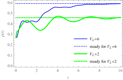
Fig. 4: (Color Online) Electron density of dot 1 as a function of time for $V_{L}=2$ and $V_{L}=6$. The straight line is the steady-state value of the electron density that is calculated from the analytical expression of the density.

The electron density oscillates in our DQD case. This cannot be seen in the case of the single dot (Fig. 2). Since the electron density is directly related to the lesser Green function $\rho_{11}(t)=-iG^{<}_{11}(t,t)$, the cause of the difference between the cases is the different behavior of the lesser Green function. In the single-dot case, the expression of the lesser Green function is Eq. (17). If we take the two times to be the same, $t_{1}=t_{2}=t$, then the imaginary part of the exponential $e^{-ih^{eff}_{11}(t_{1}-t_{0})}$ vanishes because of the factor $e^{i(h^{eff}_{11})^{*}(t_{2}-t_{0})}$. Therefore, the oscillation does not appear in the single-dot case. In the double-dot case, the expression of the lesser Green function is Eq. (63). Unlike the singe-dot case, there are two exponential functions with different exponents $k_{1}$ and $k_{2}$. Therefore, the imaginary parts of these exponential functions do not vanish and the oscillation appears.

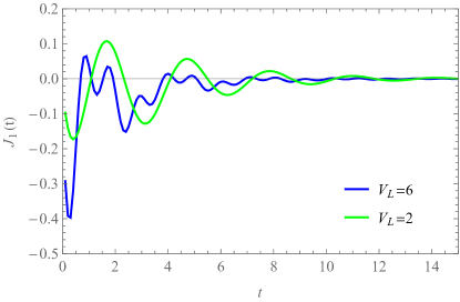
Fig. 5: (Color Online) Current from dot 1 for $V_{L}=2$ and $V_{L}=5$.

We can obtain the graph of the current from dot 1 by differentiating the electron density of dot 1. The result is shown in Fig. 5. The behavior of the current depends on the bias voltage. For the low bias of $V_{L}=2$, we can see that there is a single crest in a period. In contrast, for the high bias of $V_{L}=6$, there are two crests in a period. Because the current from dot 1 is obtained by differentiating the electron density of dot 1, this difference arises from the existence of $k_{1}$ and $k_{2}$, which are the solutions of the characteristic equation of the second-order differential equation for the retarded Green function (51). Since the necessity to investigate the second-order partial differential equations arises from the existence of the coupling between the dots, we conclude that the two wave crests in the current between the dots is a manifestation of the fact that the system consists of two subsystems.

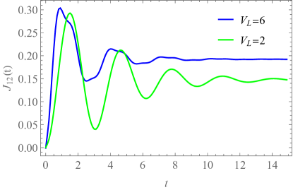
Fig. 6: (Color Online) Current between the dots for $V_{L}=2$ and $V_{L}=6$.

We also calculate the graph of the current between the dots based on Eq. (66). Fig. 6 shows the result. From the graph, we can see that the bias voltage changes the frequency of the waves. The change occurs because the bias voltage causes a phase shift of the current meaning the term $e^{-i\psi_{L}(t,t_{0})}$. We can understand this by considering the fact that the lesser Green function exists in the expression of the current from the left reservoir (65), which is a part of the current between the dots (66). In the lesser Green function (63), the pseudo self-energy and the self-energy exist, which have the term $e^{-i\psi_{L}(t,t_{0})}$. The concrete expressions of these self-energies are in Appendices A and C. Because of the term, the frequency becomes high as the bias voltage increases. In addition, we can see that the difference in the number of peaks of the waves vanishes, which we saw in the behavior of the current from dot 1(Fig. 5). This is because the current between the dots is expressed as the sum of the currents (66), and the current from the left reservoir cancels the behavior of the current from dot 1.

We also investigate the relaxation time. When a physical quantity $A(t)$ behaves as $A(t)\eqsim e^{-\frac{t}{\tau}}$, $\tau$ is called the relaxation time. The notation $\eqsim$ means that we ignore algebraic functions multiplied by the exponential. From expression (63), we can see that the relaxation time is determined by $\mathrm{min}_{{i,j}={1,2}}\mathrm{Im}[k_{i}-(k_{j})^{*}]$. Let us explain this with Eq. (63). From the first term in Eq. (63), the terms $e^{-i(k_{1}-(k_{1})^{*})t}$ and $e^{-i(k_{2}-(k_{1})^{*})t}$ appear as the exponential functions $e^{-ik_{1}t}$ and $e^{-ik_{2}t}$ exist in the right Green function (57), which is a part of $l_{1}(t)$. Similarly, $e^{-i(k_{1}-(k_{2})^{*})t}$ and $e^{-i(k_{2}-(k_{2})^{*})t}$ appear from the second term in Eq. (63). Therefore, the smallest term of $\mathrm{Im}[k_{i}-(k_{j})^{*}](i,j={1,2})$ determines the relaxation time. For the case $\epsilon_{1}=\epsilon_{2}=\epsilon$, the exponent takes the following forms:

$$\mathop{\rm min}\limits_{{i,j}={1,2}}\mathrm{Im}[k_{i}-(k_{j})^{*}]=\begin{cases}-\frac{\Gamma_{L}+\Gamma_{R}}{2}+\sqrt{\frac{1}{16}(\Gamma_{L}-\Gamma_{R})^{2}-|t_{12}|^{2}}&|t_{12}|\leq 1/4|\Gamma_{L}-\Gamma_{R}|\\ -\frac{\Gamma_{L}+\Gamma_{R}}{2}&|t_{12}|>1/4|\Gamma_{L}-\Gamma_{R}|.\end{cases}$$ (67)

The division arises because the inside of the square root in the expression for $k_{1}$ or $k_{2}$ can be both negative or positive. When we consider the case $|t_{12}|\leq 1/4|\Gamma_{L}-\Gamma_{R}|$, the relaxation time $\tau$ is $2/\left(\Gamma_{L}+\Gamma_{R}-2\sqrt{\frac{1}{16}(\Gamma_{L}-\Gamma_{R})^{2}-|t_{12}|^{2}}\right)$. Therefore, the relaxation time becomes smaller as $|t_{12}|$ increases. This is intuitively a natural result. For the case $|t_{12}|>1/4|\Gamma_{L}-\Gamma_{R}|$, however, we can see an interesting fact. In this case, $\tau$ is $2/(\Gamma_{L}+\Gamma_{R})$. This expression reveals that the relaxation time $\tau$ does not depend on $|t_{12}|$. This is against our intuition. Since the coupling strength between the dots determines the probability that an electron in a dot is transported to the other dot, we can expect that the relaxation time becomes smaller as the coupling strength between the dots increases. To test this hypothesis, we calculate the relaxation time from the numerical results and compare it with the theoretically expected value. We consider the case where the parameters take the values $\Gamma_{L}=\Gamma_{R}=1/2$, $\epsilon=1$, $V_{L}=6$, and $\beta=1$. In this situation, the relaxation time does not depend on the coupling strength $|t_{12}|>0$. In our analysis, we obtain the relaxation time numerically by fitting the data of the current from dot 1, $J_{1}$, to an exponential function.

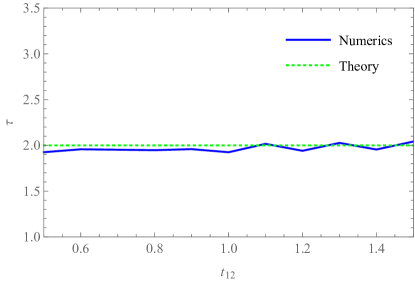
Fig. 7: (Color Online) Relaxation time for various couplings between the dots. The relaxation time takes almost the same value as the theoretically expected value of $\tau=2$.

We calculate the relaxation time for various coupling strengths of the dots $|t_{12}|$, $0.5\leq|t_{12}|\leq 1.5$. The result is shown in Fig. 7. In this case, the theoretical value is $\tau=2$. Therefore, we conclude that the relaxation time is actually constant and matches the theoretical value. This phenomenon can be understood as follows. From the representation of the retarded Green function (53), we see that the imaginary parts of $k_{1}$ and $k_{2}$ determine the lifetime of quasiparticles[34]. The forms of the imaginary parts of $k_{1}$ and $k_{2}$ depend on the square root in the expression for $k_{1}$ and $k_{2}$. Since the sign of the inside of the square root is determined by $|t_{12}|$ and $1/4|\Gamma_{L}-\Gamma_{R}|$, the lifetime of quasiparticles, or the relaxation time, depends on the parameters. Note that this behavior of the relaxation time can be seen in any temperature regime because the temperature does not appear in the above discussion. This result may be useful for manipulating the coherence time such as in quantum computation.

6 Conclusion

We have investigated the transient dynamics of double quantum dots with the nonequilibrium Green function method in the wide-band-limit approximation. As a result, we obtained the analytic expressions of the electron density of a dot, the current from dot1, and the current between the dots. Based on these results, we calculated the physical quantities numerically for the quenched case, where a constant bias voltage is suddenly applied to a reservoir. From the numerical computation, we found that a quantum fluctuation appears in the electron density and the currents. In particular, the qualitative behavior of the current from dot1 depends on the bias voltage. For a low bias voltage, there is one crest in a period of oscillation in the current. However, for a high bias voltage, the number of crests in a period changes to two. This difference arises from the existence of the coupling between the dots. In addition, we calculated the relaxation time and found that the relaxation time becomes constant when the coupling constant between the dots is sufficiently large in comparison with the difference in coupling strength between the dots and the reservoirs. This implies that if a system is an open system, we have to take the effects from the edges into consideration even when we consider a quantity in the scatterers.

Until now, we have only considered the regime where the Coulomb interaction is irrelevant. Therefore, our next goal is to investigate the transient dynamics of the double quantum dots including the Coulomb interaction. Since many interesting studies have been reported, even for the steady case, we can expect that much richer phenomena will arise from the competition of the initial correlation effects and the Coulomb interaction in the transient dynamics of double quantum dots.

Appendix A Non-perturbative Green function and the self-energy in the WBLA

A.1 Non-perturbative Green function

The non-perturbative Green function obeys the equation of motion

$$\left[i\frac{d}{dz_{1}}-\mathbf{h}_{\alpha\alpha}(z_{1})\right]\mathbf{g}_{\alpha\alpha}(z_{1},z_{2})=\mathbf{1}\delta(z_{1},z_{2}).$$

This means that the non-perturbative Green function is the Green function for the case where reservoir $\alpha$ evolves independently, or with no interaction. Then we consider the expression of the operator $d_{k\alpha}(z)$ under the Hamiltonian $\mathbf{h}_{\alpha\alpha}$. Because the time-dependent part of the Hamiltonian $V_{\alpha}(t)d^{\dagger}_{k\alpha}d_{k\alpha}$ and the remaining part $\epsilon_{k\alpha}d^{\dagger}_{k\alpha}d_{k\alpha}$ are interchangeable, the operator $d_{k\alpha}(z)$ for $z\in C_{\pm}$ is represented as

$$d_{k\alpha}(t)=d_{k\alpha}e^{-i\phi(t,t_{0})}=(d^{\dagger}_{k\alpha}(t))^{\dagger},$$

where we define the function $\phi_{k\alpha}(t,t_{0})=\epsilon_{k\alpha}(t-t_{0})+\int^{t}_{t_{0}}dsV_{\alpha}(s)$ for convenience. In the same way, the operator $d_{k\alpha}(z)$ for $z=t_{0}-i\tau\in C_{M}$ is expressed as

$$d_{k\alpha}(t_{0}-i\tau)=d_{k\alpha}e^{-(\epsilon_{k\alpha}-\mu)\tau},$$

$$d^{\dagger}_{k\alpha}(t_{0}-i\tau)=d^{\dagger}_{k\alpha}e^{(\epsilon_{k\alpha}-\mu)\tau}.$$

Note that $(d_{k\alpha}(t_{0}-i\tau))^{\dagger}\neq d^{\dagger}_{k\alpha}(t_{0}-i\tau)$. From these operators, the non-perturbative Green functions are calculated as

$$[\mathbf{g}^{r}_{\alpha\alpha}(t_{1},t_{2})]_{k,k^{\prime}}=-i\theta(t_{1}-t_{2})\delta_{kk^{\prime}}e^{-i\phi_{k\alpha}(t_{1},t_{2})},$$ (A.1)

$$[\mathbf{g}^{a}_{\alpha\alpha}(t_{1},t_{2})]_{k,k^{\prime}}=i\theta(t_{2}-t_{1})\delta_{kk^{\prime}}e^{-i\phi_{k\alpha}(t_{1},t_{2})},$$ (A.2)

$$[\mathbf{g}^{>}_{\alpha\alpha}(t_{1},t_{2})]_{k,k^{\prime}}=-i\delta_{kk^{\prime}}[1-f(\epsilon_{k\alpha}-\mu)]e^{-i\phi_{k\alpha}(t_{1},t_{2})},$$ (A.3)

$$[\mathbf{g}^{<}_{\alpha\alpha}(t_{1},t_{2})]_{k,k^{\prime}}=i\delta_{kk^{\prime}}f(\epsilon_{k\alpha}-\mu)e^{-i\phi_{k\alpha}(t_{1},t_{2})}.$$ (A.4)

For the Matsubara component, it is useful to use the representation of the Matsubara sum, which arises from the boundary conditions $\mathbf{g}_{\alpha\alpha}(z_{1},t_{0})=-\mathbf{g}_{\alpha\alpha}(z_{1},\beta)$, $\mathbf{g}_{\alpha\alpha}(t_{0},z_{2})=-\mathbf{g}_{\alpha\alpha}(\beta,z_{2})$,

$$[\mathbf{g}^{M}_{\alpha\alpha}(\tau_{1},\tau_{2})]_{k,k^{\prime}}=\delta_{kk^{\prime}}\frac{i}{\beta}\sum_{q}\frac{e^{-\omega_{q}(\tau_{1}-\tau_{2})}}{\omega_{q}-\epsilon_{k\alpha}+\mu},$$ (A.5)

where $\omega_{q}=i\pi(2q+1)/\beta$ is the Matsubara frequency and the summation over $q$ runs over all integers. The derivation is as follows. From the definition of the Matsubara Green function,

$$\left[\mathbf{g}^{M}_{\alpha\alpha}(\tau_{1},\tau_{2})\right]_{kk^{\prime}} =-i\braket{\mathcal{T}_{\tau}(d^{M}_{k\alpha}(\tau_{1})(d^{\dagger}_{k^{\prime}\alpha})^{M})}$$

$$=-i\left[\theta(\tau_{1}-\tau_{2})(1-f(\epsilon_{k\alpha}-\mu))-\theta(\tau_{2}-\tau_{1})f(\epsilon_{k\alpha}-\mu)\right]e^{-(\epsilon_{k\alpha}-\mu)(\tau_{1}-\tau_{2})}\delta_{kk^{\prime}}$$

$$(\because\mathrm{the\ expectation\ is\ taken\ in\ the\ equilibrium\ state}$$

$$=-i\left[\theta(\tau)(1-f(\epsilon_{k\alpha}-\mu))-\theta(-\tau)f(\epsilon_{k\alpha}-\mu)\right]e^{-(\epsilon_{k\alpha}-\mu)\tau}\delta_{kk^{\prime}}.(\because\tau_{1}-\tau_{2}=\tau$$

Then we use these expressions in the Fourier transform related to the Matsubara frequency:

$$\frac{1}{i}\int^{\beta}_{0}d\tau\theta(\tau)e^{(\omega_{q}-\epsilon_{k\alpha}+\mu)\tau} =i\frac{1+e^{-\beta(\epsilon_{k\alpha}-\mu)}}{\omega_{q}-\epsilon_{k\alpha}+\mu},$$

$$\frac{1}{i}\int^{\beta}_{0}d\tau\theta(-\tau)e^{(\omega_{q}-\epsilon_{k\alpha}+\mu)\tau} =0.$$

By substituting these expressions in the definition, we obtain

$$\left[\mathbf{g}^{M}_{\alpha\alpha}(\tau_{1},\tau_{2})\right]_{kk^{\prime}} =i\frac{1}{\beta}\sum_{q}e^{-\omega_{q}(\tau_{1}-\tau_{2})}(1-f(\epsilon_{k\alpha}-\mu))\left(\frac{1+e^{-\beta(\epsilon_{k\alpha}-\mu)}}{\omega_{q}-\epsilon_{k\alpha}+\mu}\right)\delta_{kk^{\prime}}$$

$$=\frac{i}{\beta}\sum_{q}\frac{e^{-\omega_{q}(\tau_{1}-\tau_{2})}}{\omega_{q}-\epsilon_{k\alpha}+\mu}.$$

The right/left non-perturbative Green functions are calculated with these results,

$$[\mathbf{g}^{\rceil}_{\alpha\alpha}(t,\tau)]_{k,k^{\prime}}=[\mathbf{g}^{M}_{\alpha\alpha}(0,\tau)]_{k,k^{\prime}}e^{-i\phi_{k\alpha}(t,t_{0})}=\delta_{kk^{\prime}}\frac{i}{\beta}e^{-i\phi_{k\alpha}(t,t_{0})}\sum_{q}\frac{e^{\omega_{q}\tau}}{\omega_{q}-\epsilon_{k\alpha}+\mu},$$ (A.6)

$$[\mathbf{g}^{\lceil}_{\alpha\alpha}(\tau,t)]_{k,k^{\prime}}=[\mathbf{g}^{M}_{\alpha\alpha}(\tau,0)]_{k,k^{\prime}}e^{i\phi_{k\alpha}(t,t_{0})}=\delta_{kk^{\prime}}\frac{i}{\beta}e^{i\phi_{k\alpha}(t,t_{0})}\sum_{q}\frac{e^{-\omega_{q}\tau}}{\omega_{q}-\epsilon_{k\alpha}+\mu}.$$ (A.7)

These are the same as in [12].

A.2 Self-energy in the WBLA

From the definition of the self-energy (34) and the expressions of the non-perturbative Green function obtained above, we can calculate the self-energy. For the retarded part, by the Fourier transform, we obtain

$$\Sigma^{r}_{11}(t_{1},t_{2}) =\theta(t_{1}-t_{2})\left[\Sigma^{>}_{11}(t_{1},t_{2})-\Sigma^{<}_{11}(t_{1},t_{2})\right]$$

$$=\theta(t_{1}-t_{2})\sum_{k,k^{\prime}}T_{1,kL}([\mathbf{g}^{>}_{LL}(t_{1},t_{2})]_{k,k^{\prime}}-[\mathbf{g}^{<}_{LL}(t_{1},t_{2})]_{k,k^{\prime}})T_{k^{\prime}L,1}\ (\because\mathrm{By\ definition(\ref{eq:34})}$$

$$=\theta(t_{1}-t_{2})\sum_{k}T_{1,kL}(-ie^{-i\phi_{kL}(t_{1},t_{2})})T_{kL,1}\ (\because\mathrm{(\ref{B.3})\ and\ (\ref{B.4})}$$

$$=-ie^{-i\psi_{L}(t_{1},t_{2})}\sum_{k}T_{1,kL}T_{kL,1}\theta(t_{1}-t_{2})e^{-i\epsilon_{kL}(t_{1}-t_{2})}$$

$$=e^{-i\psi_{L}(t_{1},t_{2})}\int\frac{d\omega}{2\pi}e^{-i\omega(t_{1}-t_{2})}\sum_{k}\frac{T_{1,k\alpha}T_{kL,1}}{\omega+i0-\epsilon_{kL}}\ (\because\mathrm{From\ the\ formula\ below}$$

$$=e^{-i\psi_{\alpha}(t_{1},t_{2})}\int\frac{d\omega}{2\pi}e^{-i\omega(t_{1}-t_{2})}\left[\Lambda_{L}(\omega)-\frac{i}{2}\Gamma_{L}(\omega)\right]\ (\because\frac{1}{x\pm i0}=\mathcal{P}\left(\frac{1}{x}\right)\mp i\pi\delta(x),$$

where we define

$$\Lambda_{L}(\omega)=\mathcal{P}\int\frac{d{\omega}^{\prime}}{2\pi}\frac{\Gamma_{L}(\omega^{\prime})}{\omega-\omega^{\prime}},$$

$$\Gamma_{L}(\omega)=2\pi\sum_{k}T_{1,kL}T_{kL,1}\delta(\epsilon_{kL}-\omega),$$

and $\mathcal{P}$ represents the Cauchy principal part. In the derivation, we use the Fourier transformation which is defined as $F(\omega)=\int^{\infty}_{-\infty}dtf(t)e^{i\omega t}$. The inverse Fourier transform is expressed as $f(t)=\int^{\infty}_{-\infty}\frac{d\omega}{2\pi}F(\omega)e^{-i\omega t}$. In this definition, the Fourier transformation of $\theta(t)e^{-iat},a\in\mathbf{R}$ is expressed as

$$\int^{\infty}_{-\infty}dt\theta(t)e^{-iat}e^{i\omega t} =\lim_{\delta\rightarrow 0^{+}}\int^{\infty}_{-\infty}dt\theta(t)e^{-(\delta-i(\omega-a))t}\ (\because\omega\rightarrow\omega+i\delta$$

$$=\lim_{\delta\rightarrow 0^{+}}\int^{\infty}_{0}dte^{-\delta t+i(\omega-a)t}$$

$$=\lim_{\delta\rightarrow 0^{+}}\left[\frac{1}{-\delta+i(\omega-a)}e^{-\delta t+i(\omega-a)t}\right]^{\infty}_{0}$$

$$=\lim_{\delta\rightarrow 0^{+}}\frac{-1}{-\delta+i(\omega-a)}$$

$$=\lim_{\delta\rightarrow 0^{+}}-\frac{1}{i}\frac{1}{\omega+i\delta-a}$$

$$=:-\frac{1}{i}\frac{1}{\omega+i0-a}.$$

Therefore, we obtain the formula $\theta(t_{1}-t_{2})e^{-i\epsilon_{kL}(t_{1}-t_{2})}=\int^{\infty}_{-\infty}\frac{d\omega}{2\pi}e^{-i\omega(t_{1}-t_{2})}\frac{i}{\omega+i0-\epsilon_{kL}}$. In the WBLA, the line width $\Gamma_{L}(\omega)$ does not depend on the energy $\omega$ and $\Lambda_{L}(\omega)$ becomes $0$: $\Gamma_{L}(\omega)\sim\Gamma_{L}$, $\Lambda_{L}=0$. Then, the retarded self-energy in the WBLA takes the form

$$\Sigma^{r}_{11}(t_{1},t_{2})=-\frac{i}{2}\Gamma_{L}\delta(t_{1}-t_{2}),$$

which is Eq. (LABEL:eq:39). Other self-energies are calculated similarly and the results are

$$\Sigma^{M}_{11}(\tau_{1},\tau_{2}) =-\frac{\Gamma_{L}}{2\beta}\sum_{q}\xi_{q}e^{-\omega_{q}(\tau_{1}-\tau_{2})},$$ (A.8)

$$\Sigma^{M}_{22}(\tau_{1},\tau_{2}) =-\frac{\Gamma_{R}}{2\beta}\sum_{q}\xi_{q}e^{-\omega_{q}(\tau_{1}-\tau_{2})},$$ (A.9)

$$\Sigma^{<}_{11}(t_{1},t_{2}) =i\Gamma_{L}e^{-i\psi_{L}(t_{1},t_{2})}\int\frac{d\omega}{2\pi}f(\omega-\mu)e^{-i\omega(t_{1}-t_{2})},$$ (A.10)

$$\Sigma^{<}_{22}(t_{1},t_{2}) =i\Gamma_{R}e^{-i\psi_{R}(t_{1},t_{2})}\int\frac{d\omega}{2\pi}f(\omega-\mu)e^{-i\omega(t_{1}-t_{2})},$$ (A.11)

$$\Sigma^{>}_{11}(t_{1},t_{2}) =-i\Gamma_{L}e^{-i\psi_{L}(t_{1},t_{2})}\int\frac{d\omega}{2\pi}[1-f(\omega-\mu)]e^{-i\omega(t_{1}-t_{2})},$$ (A.12)

$$\Sigma^{>}_{22}(t_{1},t_{2}) =-i\Gamma_{R}e^{-i\psi_{R}(t_{1},t_{2})}\int\frac{d\omega}{2\pi}[1-f(\omega-\mu)]e^{-i\omega(t_{1}-t_{2})},$$ (A.13)

$$\Sigma^{\lceil}_{11}(\tau,t) =\frac{i}{\beta}\Gamma_{L}e^{i\psi_{L}(t,t_{0})}\sum_{q}e^{-{\omega}_{q}\tau}\int\frac{d\omega}{2\pi}\frac{e^{i\omega(t-t_{0})}}{\omega_{q}-\omega+\mu},$$ (A.14)

$$\Sigma^{\lceil}_{22}(\tau,t) =\frac{i}{\beta}\Gamma_{R}e^{i\psi_{R}(t,t_{0})}\sum_{q}e^{-{\omega}_{q}\tau}\int\frac{d\omega}{2\pi}\frac{e^{i\omega(t-t_{0})}}{\omega_{q}-\omega+\mu},$$ (A.15)

$$\Sigma^{\rceil}_{11}(\tau,t) =\frac{i}{\beta}\Gamma_{L}e^{-i\psi_{L}(t,t_{0})}\sum_{q}e^{{\omega}_{q}\tau}\int\frac{d\omega}{2\pi}\frac{e^{-i\omega(t-t_{0})}}{\omega_{q}-\omega+\mu},$$ (A.16)

$$\Sigma^{\rceil}_{22}(\tau,t) =\frac{i}{\beta}\Gamma_{R}e^{-i\psi_{R}(t,t_{0})}\sum_{q}e^{{\omega}_{q}\tau}\int\frac{d\omega}{2\pi}\frac{e^{-i\omega(t-t_{0})}}{\omega_{q}-\omega+\mu}.$$ (A.17)

Appendix B Modified Langreth rule for the pseudo self-energy in the WBLA

The Langreth rule[37] are written as

$$\Sigma^{r}_{11}(t_{1},t_{2})=\Sigma^{--}_{11}(t_{1},t_{2})-\Sigma^{<}_{11}(t_{1},t_{2}),$$ (B.1)

$$\Sigma^{a}_{11}(t_{1},t_{2})=\Sigma^{--}_{11}(t_{1},t_{2})-\Sigma^{>}_{11}(t_{1},t_{2}).$$ (B.2)

The rules express the relations between the retarded or the advanced part of the self-energy and other parts of the self-energy. The rules are derived straightforwardly from the fact that the self-energies are defined on contour $\gamma$. Therefore, the rules also hold for other quantities defined on the contour such as the nonequilibrium Green functions. Since the pseudo self-energies $\tilde{\Sigma}_{11}$ are expressed in terms of the quantities on the contour, one may expect the pseudo self-energy to follow the Langreth rule. However, we cannot apply the Langreth rule to the pseudo self-energies. This is because there is a product of quantities that depends on contour $\gamma$ in its definition (37). Instead, the following modified Langreth rules hold for the pseudo self-energy:

$$\tilde{\Sigma}^{r}_{11}=\tilde{\Sigma}^{--}_{11}(t_{1},t_{2})-\tilde{\Sigma}^{<}_{11}(t_{1},t_{2})+\left(\Sigma^{r}_{11}\cdot\Sigma^{r}_{22}\right)_{(t_{1},t_{2})}-\delta(t_{1}-t_{2})(\mathbf{h}_{1L}\mathbf{h}_{L1}+\mathbf{h}_{2R}\mathbf{h}_{R2}),$$ (B.3)

$$\tilde{\Sigma}^{a}_{11}=\tilde{\Sigma}^{--}_{11}(t_{1},t_{2})-\tilde{\Sigma}^{>}_{11}(t_{1},t_{2})+\left(\Sigma^{r}_{22}\cdot\Sigma^{r}_{11}\right)_{(t_{1},t_{2})}-\delta(t_{1}-t_{2})(\mathbf{h}_{1L}\mathbf{h}_{L1}+\mathbf{h}_{2R}\mathbf{h}_{R2}).$$ (B.4)

When we calculate the quantities including the pseudo self-energies, we use the modified Langreth rules.

Their derivation is as follows. To derive the modified Langreth rule (B.3), we compare the expression for the retarded part of the pseudo self-energy $\tilde{\Sigma}^{r}_{11}:=\theta(t_{1}-t_{2})(\tilde{\Sigma}^{>}_{11}-\tilde{\Sigma}^{<}_{11})$ and these for other parts of the pseudo self-energy $\tilde{\Sigma}^{--}_{11}-\tilde{\Sigma}^{<}_{11}$. By substituting the equation of motion for the non-perturbative Green function into the derivative of the self-energies in the definition of the pseudo self-energy (37), we obtain the expression

$$\tilde{\Sigma}_{11}(z_{1},z_{2})=\mathbf{h}_{1L}\mathbf{h}_{LL}\mathbf{g}_{LL}(z_{1},z_{2})\mathbf{h}_{L1}+\mathbf{h}_{2R}\mathbf{h}_{RR}\mathbf{g}_{RR}(z_{1},z_{2})\mathbf{h}_{R2}-\epsilon_{1}\Sigma_{11}(z_{1},z_{2})-\epsilon_{2}\Sigma_{22}(z_{1},z_{2})\\ -\int_{\gamma}d\bar{z}\Sigma_{22}(z_{1},\bar{z})\Sigma_{11}(\bar{z},z_{2})+\delta(z_{1},z_{2})(\mathbf{h}_{1L}\mathbf{h}_{L1}+\mathbf{h}_{2R}\mathbf{h}_{R2}).$$ (68)

From Eq. (68), we can obtain expressions of $\tilde{\Sigma}^{r}_{11}$ and $\tilde{\Sigma}^{--}_{11}-\tilde{\Sigma}^{<}_{11}$. If there were only the first four terms in Eq. (68), we could apply the ordinary Langreth rule because the non-perturbative Green function and the self-energy satisfy the standard Langreth rule. Howecer, a modification is necessary due to the existence of the fifth term $\int_{\gamma}d\bar{z}\Sigma_{22}(z_{1},\bar{z})\Sigma_{11}(\bar{z},z_{2})$ and the sixth term $\delta(z_{1},z_{2})(\mathbf{h}_{1L}\mathbf{h}_{L1}+\mathbf{h}_{2R}\mathbf{h}_{R2})$. Therefore, we only consider the expressions of the fifth and the sixth terms of $\tilde{\Sigma}^{r}_{11}$ and $\tilde{\Sigma}^{--}_{11}-\tilde{\Sigma}^{<}_{11}$ and compare them. In fact, the fifth term for $\tilde{\Sigma}^{r}_{11}$ is 0 in the WBLA,

$$\theta(t_{1}-t_{2})\int_{\gamma}d\bar{z}(\Sigma_{22}^{+\ }(t_{1},\bar{z})\Sigma_{11}^{\ -}(\bar{z},t_{2})-\Sigma_{22}^{-}(t_{1},\bar{z})\Sigma_{11}^{\ +}(\bar{z},t_{2})=0,$$ (B.6)

where we use the expression of the self-energy in the WBLA, which is calculated in Appendix A. The sixth term vanishes for the pseudo retarded self-energy due to the Heaviside function in the definition. For $\tilde{\Sigma}^{--}_{11}-\tilde{\Sigma}^{<}_{11}$, the fifth term is written as

$$\int_{\gamma}d\bar{z}(\Sigma_{22}^{-}(t_{1},\bar{z})\Sigma_{11}^{\ -}(\bar{z},t_{2})-\Sigma_{22}^{-}(t_{1},\bar{z})\Sigma_{11}^{\ +}(\bar{z},t_{2})=\left(\Sigma^{r}_{22}\cdot\Sigma^{r}_{11}\right)_{(t_{1},t_{2})},$$ (B.7)

where we use the Langreth rule. The notation $\Sigma_{22}^{-}(t_{1},\bar{z})$ means that the argument $z_{1}$ is on contour $C_{-}$ and the argument $z_{2}$ is not identified where it is on contour $\gamma$. The sixth term remains unchanged. Therefore, we can conclude that the difference between $\tilde{\Sigma}^{--}_{11}-\tilde{\Sigma}^{<}_{11}$ and $\tilde{\Sigma}^{r}_{11}$ is $\left(\Sigma^{r}_{22}\cdot\Sigma^{r}_{11}\right)_{(t_{1},t_{2})}-\delta(t_{1}-t_{2})(\mathbf{h}_{1L}\mathbf{h}_{L1}+\mathbf{h}_{2R}\mathbf{h}_{R2})$. This means that the modified Langreth rule (B.3) holds. The modified Langreth rule for the advanced pseudo self-energy (B.4) is derived in the same way.

Appendix C Pseudo self-energy in the WBLA

C.1 Matsubara pseudo self-energy

From the definition of the pseudo self-energy (37), we obtain

$$\tilde{\Sigma}^{M}_{11}(\tau_{1},\tau_{2}) =\mathbf{h}_{1L}\left(-\frac{d}{d\tau_{1}}\right)\mathbf{g}^{M}_{LL}(\tau_{1},\tau_{2})\mathbf{h}_{L1}+\mathbf{h}_{2R}\mathbf{g}^{M}_{LL}(\tau_{1},\tau_{2})\left(\frac{\overleftarrow{d}}{d\tau_{2}}\right)\mathbf{h}_{R2}$$

$$\ -(\epsilon_{1}-\mu)\Sigma^{M}_{22}(\tau_{1},\tau_{2})-(\epsilon_{2}-\mu)\Sigma^{M}_{11}(\tau_{1},\tau_{2})-\left(\Sigma_{22}*\Sigma_{11}\right)_{(\tau_{1},\tau_{2})}$$

$$=(\mathrm{i})+(\mathrm{ii})+(\mathrm{iii})+(\mathrm{iv})+(\mathrm{v}).$$ (C.1)

The first term is computed as

$$(\mathrm{i}) =\Gamma_{L}\frac{i}{\beta}\sum_{q}\int\frac{d\omega}{2\pi}\frac{\omega_{q}}{\omega_{q}-\omega+\mu}e^{-\omega_{q}(\tau_{1}-\tau_{2})}$$

$$=-\frac{\Gamma_{L}}{2\beta}\sum_{q}\omega_{q}\xi_{q}e^{-\omega_{q}(\tau_{1}-\tau_{2})},$$ (C.2)

where we use the expression

$$\int\frac{d\omega}{2\pi}\frac{1}{\omega_{q}-\omega+\mu}=\frac{i}{2}\xi_{q}.$$

The function $\xi_{q}$ is defined as $\xi_{q}=1$ (Im $\omega_{q}<0$), $-1$ (Im $\omega_{q}>0$). In the same way, the second term is written as

$$(\mathrm{ii})=-\frac{\Gamma_{R}}{2\beta}\sum_{q}\omega_{q}\xi_{q}e^{-\omega_{q}(\tau_{1}-\tau_{2})}.$$ (C.3)

Using the expressions for the Matsubara self-energies (A.8) and (A.9) calculated in Appendix A, we obtain

$$(\mathrm{iii}) =(\epsilon_{1}-\mu)\frac{\Gamma_{R}}{2\beta}\sum_{q}\omega_{q}e^{-\omega_{q}(\tau_{1}-\tau_{2})},$$ (C.4)

$$(\mathrm{iv}) =(\epsilon_{2}-\mu)\frac{\Gamma_{L}}{2\beta}\sum_{q}\omega_{q}e^{-\omega_{q}(\tau_{1}-\tau_{2})}.$$ (C.5)

The fifth term is calculated using the relation $\int^{\beta}_{0}d\tau e^{-(\omega_{q}-\omega_{q}^{\prime})\tau}=\beta\delta_{q,q^{\prime}}$ and the result is

$$(\mathrm{v})=i\frac{\Gamma_{L}\Gamma_{R}}{4\beta}\sum_{q}e^{-\omega_{q}(\tau_{1}-\tau_{2})}.$$ (C.6)

Using expressions from Eq. (C.2)-(C.6), we obtain the Matsubara pseudo self-energy (52) as

$$\tilde{\Sigma}^{M}_{11}(\tau_{1},\tau_{2})=\sum_{q}e^{-\omega_{q}(\tau_{1}-\tau_{2})}\big{[}-\frac{\xi_{q}}{2\beta}\{(\omega_{q}-\epsilon_{1}+\mu)\Gamma_{R}+(\omega_{q}-\epsilon_{2}+\mu)\Gamma_{L}\}+i\frac{\Gamma_{L}\Gamma_{R}}{4\beta}\big{]}.$$ (C.7)

C.2 Retarded/advanced pseudo self-energy

The retarded pseudo self-energy is defined as $\tilde{\Sigma}^{r}_{11}(t_{1},t_{2})=\theta(t_{1}-t_{2})(\tilde{\Sigma}^{>}_{11}(t_{1},t_{2})-\tilde{\Sigma}^{<}_{11}(t_{1},t_{2}))$. Using the definition of the pseudo self-energy (37), this is written in the form

$$\tilde{\Sigma}^{r}_{11}(t_{1},t_{2}) =\theta(t_{1}-t_{2})\bigg{[}\left(i\frac{d}{dt_{1}}-\epsilon_{2}\right)\left(\Sigma^{>}_{11}(t_{1},t_{2})-\Sigma^{<}_{11}(t_{1},t_{2})\right)$$

$$\quad+\left(\Sigma^{>}_{22}(t_{1},t_{2})-\Sigma^{<}_{22}(t_{1},t_{2})\right)\left(-i\frac{\overleftarrow{d}}{dt_{2}}-\epsilon_{1}\right)$$

$$\qquad-\int_{\gamma}d\bar{z}(\Sigma_{22}^{+\ }(t_{1},\bar{z})\Sigma_{11}^{\ -}(\bar{z},t_{2})-\Sigma_{22}^{-}(t_{1},\bar{z})\Sigma_{11}^{\ +}(\bar{z},t_{2})\bigg{]}$$

$$=(\mathrm{vi})+(\mathrm{vii})+(\mathrm{viii}).$$ (C.8)

Using the definition of the retarded self-energy, we rewrite the first term $(\mathrm{vi})$ as

$$\theta(t_{1}-t_{2})\left(i\frac{d}{dt_{1}}-\epsilon_{2}\right)\left(\Sigma^{>}_{11}(t_{1},t_{2})-\Sigma^{<}_{11}(t_{1},t_{2})\right)=\left(i\frac{d}{dt_{1}}-\epsilon_{2}\right)\Sigma^{r}_{11}(t_{1},t_{2})\\ -i\delta(t_{1}-t_{2})\left(\Sigma^{>}_{11}(t_{1},t_{2})-\Sigma^{<}_{11}(t_{1},t_{2})\right).$$ (69)

Using the expressions for the self-energies, (A.10) and (A.12), we obtain

$$\left(\Sigma^{>}_{11}(t_{1},t_{2})-\Sigma^{<}_{11}(t_{1},t_{2})\right)=-i\mathbf{h}_{1L}\mathbf{h}_{L1}e^{-i\psi_{kL}(t_{1},t_{2})}.$$

Therefore, Eq. (69) is expressed in the form

$$\theta(t_{1}-t_{2})\left(i\frac{d}{dt_{1}}-\epsilon_{2}\right)\left(\Sigma^{>}_{11}(t_{1},t_{2})-\Sigma^{<}_{11}(t_{1},t_{2})\right)=\left(i\frac{d}{dt_{1}}-\epsilon_{2}\right)\Sigma^{r}_{11}(t_{1},t_{2})-\mathbf{h}_{1L}\mathbf{h}_{L1}\delta(t_{1}-t_{2}).$$ (C.10)

In the same way, $(\mathrm{vii})$ is represented as

$$\theta(t_{1}-t_{2})\left(\Sigma^{>}_{22}(t_{1},t_{2})-\Sigma^{<}_{22}(t_{1},t_{2})\right)\left(-i\frac{\overleftarrow{d}}{dt_{2}}-\epsilon_{1}\right)=\Sigma^{r}_{22}(t_{1},t_{2})\left(-i\frac{\overleftarrow{d}}{dt_{2}}-\epsilon_{1}\right)-\mathbf{h}_{2R}\mathbf{h}_{R2}\delta(t_{1}-t_{2}).$$ (C.11)

Then we use the expression for the retarded self-energy in the WBLA (LABEL:eq:39). By substituting the expression into Eqs. (C.10) and (C.11), we obtain

$$\theta(t_{1}-t_{2})\bigg{[}\left(i\frac{d}{dt_{1}}-\epsilon_{2}\right)\left(\Sigma^{>}_{11}(t_{1},t_{2})-\Sigma^{<}_{11}(t_{1},t_{2})\right)+\left(\Sigma^{>}_{22}(t_{1},t_{2})-\Sigma^{<}_{22}(t_{1},t_{2})\right)\left(-i\frac{\overleftarrow{d}}{dt_{2}}-\epsilon_{1}\right)\bigg{]}$$

$$=\frac{1}{2}(\Gamma_{L}+\Gamma_{R})\frac{d}{d(t_{1}-t_{2})}\delta(t_{1}-t_{2})+\frac{i}{2}(\epsilon_{2}\Gamma_{L}+\epsilon_{1}\Gamma_{R})\delta(t_{1}-t_{2})$$

$$\qquad-(\mathbf{h}_{1L}\mathbf{h}_{L1}+\mathbf{h}_{2R}\mathbf{h}_{R2})\delta(t_{1}-t_{2}).$$ (C.12)

By the substitution of Eqs. (C.12) and (B.7) in Eq. (C.8), we obtain the expression of the retarded pseudo self-energy (40). The advanced pseudo self-energy is calculated in the same way and the result is

$$\tilde{\Sigma}^{a}_{11}(t_{1},t_{2}) :=-\theta(t_{2}-t_{1})(\tilde{\Sigma}^{>}_{11}(t_{1},t_{2})-\tilde{\Sigma}^{<}_{11}(t_{1},t_{2})$$

$$=-\frac{1}{2}(\Gamma_{L}+\Gamma_{R})\frac{d}{d(t_{1}-t_{2})}\delta(t_{1}-t_{2})-\frac{i}{2}(\epsilon_{2}\Gamma_{L}+\epsilon_{1}\Gamma_{R})\delta(t_{1}-t_{2})$$ (C.13)

$$-(\mathbf{h}_{1L}\mathbf{h}_{L1}+\mathbf{h}_{2R}\mathbf{h}_{R2})\delta(t_{1}-t_{2}).$$

C.3 Left/right pseudo self-energy

From the definition (37), the left pseudo self-energy is represented as

$$\tilde{{\Sigma}^{\lceil}}_{11}(\tau,t) =\left(-\frac{d}{d\tau}-\epsilon_{2}+\mu\right)\Sigma^{\lceil}_{11}(\tau,t)+\Sigma^{\lceil}_{22}(\tau,t)\left(-i\frac{\overleftarrow{d}}{dt}-\epsilon_{1}\right)$$

$$-\int_{\gamma}d\bar{z}\Sigma_{22}(\tau,\bar{z})\Sigma_{11}(\bar{z},t)$$

$$=\mathrm{(ix)+(x)+(xi)}.$$ (C.14)

From the expressions (A.14) and (A.15) for the left self-energy in the WBLA, the first and second terms are written as

$$\mathrm{(ix)} =\frac{i}{\beta}\Gamma_{L}e^{i\psi_{L}(t,t_{0})}\sum_{q}(\omega_{q}-\epsilon_{2}+\mu)e^{-\omega_{q}\tau}\int\frac{d\omega}{2\pi}\frac{e^{i\omega(t-t_{0})}}{\omega_{q}-\omega+\mu},$$ (C.15)

$$\mathrm{(x)} =\frac{i}{\beta}\Gamma_{R,11}e^{i\psi_{R}(t,t_{0})}\sum_{q}e^{-\omega_{q}\tau}\int\frac{d\omega}{2\pi}\frac{\omega+V_{R}(t)-\epsilon_{1}}{\omega_{q}-\omega+\mu}e^{i\omega(t-t_{0})}.$$ (C.16)

Using the Langreth rule and the expressions for the retarded and advanced self-energy in the WBLA (LABEL:eq:39), we obtain

$$\mathrm{(xi)}=-\frac{i}{2}\Gamma_{L}(\tau,t)\Sigma^{\lceil}_{22}-\left(\Sigma^{M}_{22}*\Sigma^{\lceil}_{11}\right)_{(\tau,t)}.$$ (C.17)

We can derive the expression of the left pseudo self-energy from Eqs. (C.14)-(C.16) as

$$\tilde{\Sigma}^{\lceil}_{11}(\tau_{1},t_{2})=\frac{i}{\beta}\Gamma_{L}e^{i\psi_{L}(t_{1},t_{0})}\sum_{q}(\omega_{q}-\epsilon_{2}+\mu)e^{-\omega_{q}\tau}\int\frac{d\omega}{2\pi}\frac{e^{i\omega(t-t_{0})}}{\omega_{q}-\omega+\mu}+\frac{i}{\beta}\Gamma_{R}e^{i\psi_{R}(t_{1},t_{0})}\\ \times\sum_{q}e^{-\omega_{q}\tau}\int\frac{d\omega}{2\pi}\frac{\omega+V_{R}(t)-\epsilon_{1}}{\omega_{q}-\omega+\mu}e^{i\omega(t-t_{0})}-\frac{i}{2}\Gamma_{L}\Sigma^{\lceil}_{22}(\tau_{1},t_{2})-\left(\Sigma^{M}_{22}*\Sigma^{\lceil}_{11}\right)_{(\tau_{1},t_{2})}.$$ (70)

The right pseudo self-energy is derived in the same way as the left pseudo self-energy and it is expressed as

$$\tilde{\Sigma}^{\rceil}_{11}(t_{1},\tau_{2})=\frac{i}{\beta}\Gamma_{L}e^{-i\psi_{L}(t_{1},t_{0})}\sum_{q}e^{\omega_{q}\tau}\int\frac{d\omega}{2\pi}\frac{\omega+V_{L}(t)-\epsilon_{2}}{\omega_{q}-\omega+\mu}e^{-i\omega(t-t_{0})}+\frac{i}{\beta}\Gamma_{R}e^{-i\psi_{R}(t_{1},t_{0})}\\ \times\sum_{q}(\omega_{q}-\epsilon_{1}+\mu)e^{\omega_{q}\tau}\int\frac{d\omega}{2\pi}\frac{e^{-i\omega(t-t_{0})}}{\omega_{q}-\omega+\mu}+\frac{i}{2}\Gamma_{R}\Sigma^{\rceil}_{11}(t_{1},\tau_{2})-\left(\Sigma^{\rceil}_{22}*\Sigma^{M}_{11}\right)_{(t_{1},\tau_{2})}.$$ (71)

C.4 Lesser/greater pseudo self-energy

From definition (37), the lesser pseudo self-energy is represented as

$$\tilde{\Sigma}^{<}_{11}(\tau,t) =\left(i\frac{d}{dt}-\epsilon_{2}\right)\Sigma^{<}_{11}(t_{1},t_{2})+\Sigma^{<}_{22}(t_{1},t_{2})\left(-i\frac{\overleftarrow{d}}{dt_{2}}-\epsilon_{1}\right)$$

$$-\int_{\gamma}d\bar{z}\Sigma^{-\ }_{22}(t_{1},\bar{z})\Sigma^{\ +}_{11}(\bar{z},t_{2})$$

$$=\mathrm{(xii)+(xiii)+(xiv)}.$$ (C.20)

By differentiating the representations, (A.10) and (A.11), of the left self-energy in the WBLA, we obtain

$$\mathrm{(xii)} =i\Gamma_{L}e^{-i\psi_{L}(t_{1},t_{2})}\int\frac{d\omega}{2\pi}(\omega+V_{L}(t_{1})-\epsilon_{2})f(\omega-\mu)e^{-i\omega(t_{1}-t_{2})},$$ (C.21)

$$\mathrm{(xiii)} =i\Gamma_{R}e^{-i\psi_{R}(t_{1},t_{2})}\int\frac{d\omega}{2\pi}(\omega+V_{R}(t_{2})-\epsilon_{1})f(\omega-\mu)e^{-i\omega(t_{1}-t_{2})}.$$ (C.22)

Using the expressions for the retarded/advanced self-energies in the WBLA (LABEL:eq:39) and the Langreth rule, the third term is written as

$$\mathrm{(xiv)}=\frac{i}{2}\left(\Gamma_{R}\Sigma^{<}_{11}-\Gamma_{L}\Sigma^{<}_{22}\right)-\left(\Sigma^{\rceil}_{22}*\Sigma^{\lceil}_{11}\right)_{(t_{1},t_{2})}.$$

Actually, the second term in the representation above equals to 0:

$$\left(\Sigma^{\rceil}_{22}*\Sigma^{\lceil}_{11}\right)_{(t_{1},t_{2})} =-i\int^{\beta}_{0}d\tau\frac{i}{\beta}\Gamma_{R}e^{-i\psi_{R}(t_{1},t_{0})}\sum_{q}e^{\omega_{q}\tau}\frac{d\omega}{2\pi}\frac{e^{-i\omega(t_{1}-t_{2})}}{\omega_{q}-\omega+\mu}$$

$$\qquad\times\frac{i}{\beta}\Gamma_{L}e^{i\psi_{L}(t_{2},t_{0})}\sum_{q^{\prime}}e^{-\omega_{q^{\prime}}\tau}\frac{d\omega}{2\pi}\frac{e^{-i\omega(t_{1}-t_{2})}}{\omega_{q^{\prime}}-\omega+\mu}$$

$$=0,$$

where we use the expressions for the left/right self-energies in the WBLA (A.14) and (A.17). From these above results, we derive the following expression for the lesser pseudo self-energy:

$$\tilde{\Sigma}^{<}_{11}(t_{1},t_{2})=i\Gamma_{L}e^{-i\psi_{L}(t_{1},t_{0})}\int\frac{d\omega}{2\pi}(\omega+V_{L}(t_{1})-\epsilon_{2})f(\omega-\mu)e^{-i\omega(t-t_{0})}+i\Gamma_{R}e^{-i\psi_{R}(t_{1},t_{0})}\\ \int\frac{d\omega}{2\pi}(\omega+V_{R}(t_{2})-\epsilon_{1})f(\omega-\mu)e^{-i\omega(t-t_{0})}+\frac{i}{2}\left(\Gamma_{R}\Sigma^{<}_{11}(t_{1},t_{2})-\Gamma_{L}\Sigma^{<}_{22}(t_{1},t_{2})\right).$$ (72)

The greater pseudo self-energy is calculated in the same way as

$$\tilde{\Sigma}^{>}_{11}(t_{1},t_{2})=-i\Gamma_{L}e^{-i\psi_{L}(t_{1},t_{0})}\int\frac{d\omega}{2\pi}(\omega+V_{L}(t_{1})-\epsilon_{2})[1-f(\omega-\mu)]e^{-i\omega(t-t_{0})}\\ -i\Gamma_{R}e^{-i\psi_{R}(t_{1},t_{0})}\int\frac{d\omega}{2\pi}(\omega+V_{R}(t_{2})-\epsilon_{1})[1-f(\omega-\mu)]e^{-i\omega(t-t_{0})}\\ +\frac{i}{2}\left(\Gamma_{R}\Sigma^{>}_{11}(t_{1},t_{2})-\Gamma_{L}\Sigma^{>}_{22}(t_{1},t_{2})\right).$$ (73)

Appendix D Derivation of the second-order partial differential equation

D.1 Lesser Green function

Here, we derive the second-order partial differential equation for the lesser Green function (35). The derivation starts from the equations of motion for $G_{11}$ and $G_{21}$ of the lesser part:

$$\left[i\frac{d}{dt_{1}}-\epsilon_{1}\right]G^{<}_{11}(t_{1},t_{2}) =\int_{\gamma}d\bar{z}\Sigma^{-\ }_{11}(t_{1},\bar{z})G^{\ +}_{11}(\bar{z},t_{2})+t_{12}G^{<}_{21}(t_{1},t_{2}),$$ (D.1)

$$\left[i\frac{d}{dt_{1}}-\epsilon_{2}\right]G^{<}_{21}(t_{1},t_{2}) =\int_{\gamma}d\bar{z}\Sigma^{-\ }_{22}(t_{1},\bar{z})G^{\ +}_{21}(\bar{z},t_{2})+t_{21}G^{<}_{11}(t_{1},t_{2}).$$ (D.2)

To substitute the differential equation for $G_{21}$ into the equation for $G_{11}$, we rewrite Eq. (D.1) in the form

$$G^{<}_{21}(t_{1},t_{2}) =\frac{1}{t_{12}}\bigg{\{}\left[i\frac{d}{dt_{1}}-\epsilon_{1}\right]G^{<}_{11}(t_{1},t_{2})-\int_{\gamma}d\bar{z}\Sigma^{-\ }_{11}(t_{1},\bar{z})G^{\ +}_{11}(\bar{z},t_{2})\bigg{\}},$$ (D.3)

$$i\frac{d}{dt_{1}}G^{<}_{21}(t_{1},t_{2}) =\frac{1}{t_{12}}\bigg{\{}\left[-\frac{d^{2}}{dt^{2}_{1}}-i\epsilon_{1}\frac{d}{dt_{1}}\right]G^{<}_{11}(t_{1},t_{2})-i\int_{\gamma}d\bar{z}\frac{d}{dt_{1}}\Sigma^{-\ }_{11}(t_{1},\bar{z})G^{\ +}_{11}(\bar{z},t_{2})\bigg{\}}.$$ (D.4)

By substituting Eqs. (D.3) and (D.4) into Eq. (D.2) and multiplying by $t_{12}$, we obtain

$$\bigg{[}-\frac{d^{2}}{dt^{2}_{1}}-i(\epsilon_{1}+\epsilon_{2})\frac{d}{dt_{1}}+(\epsilon_{1}\epsilon_{2}-t_{12}t_{21})\bigg{]}G^{<}_{11}(t_{1},t_{2})\\ =\int_{\gamma}d\bar{z}(i\frac{d}{dt_{1}}-\epsilon_{2})\Sigma^{-\ }_{11}(t_{1},\bar{z})G^{\ +}_{11}(\bar{z},t_{2})+t_{12}\int_{\gamma}d\bar{z}\Sigma^{-\ }_{22}(t_{1},\bar{z})G^{\ +}_{21}(\bar{z},t_{2}).$$ (74)

With the Langreth rule, the rightmost term is expressed as

$$t_{12}\int_{\gamma}d\bar{z}\Sigma^{-\ }_{22}(t_{1},\bar{z})G^{\ +}_{21}(\bar{z},t_{2})=t_{12}\left(\Sigma^{--}_{22}\cdot G^{<}_{21}-\Sigma^{<}_{22}\cdot G^{++}_{21}+\Sigma^{\rceil}_{12}*G^{\lceil}_{21}\right)_{(t_{1},t_{2})}.$$ (D.6)

Using the equation of motion for $G_{11}$ (32), we rewrite $G_{21}$ in Eq. (D.6) in terms of $G_{11}$. From Eq. (32), we obtain

$$G^{<}_{21}(t_{1},t_{2})=\frac{1}{t_{12}}\bigg{\{}\left[i\frac{d}{dt_{1}}-\epsilon_{1}\right]G^{<}_{11}(t_{1},t_{2})-\int_{\gamma}d\bar{z}\Sigma^{-\ }_{11}(t_{1},\bar{z})G^{\ +}_{11}(\bar{z},t_{2})\bigg{\}},$$

$$G^{++}_{21}(t_{1},t_{2})=\frac{1}{t_{12}}\bigg{\{}\left[i\frac{d}{dt_{1}}-\epsilon_{1}\right]G^{++}_{11}(t_{1},t_{2})-\int_{\gamma}d\bar{z}\Sigma^{+\ }_{11}(t_{1},\bar{z})G^{\ +}_{11}(\bar{z},t_{2})-\delta(t_{1}-t_{2})\bigg{\}},$$

$$G^{\rceil}_{21}(\tau_{1},t_{2})=\frac{1}{t_{12}}\bigg{\{}\left[-\frac{d}{d\tau_{1}}-\epsilon_{1}+\mu\right]G^{\rceil}_{11}(\tau_{1},t_{2})-\int_{\gamma}d\bar{z}\Sigma_{11}(\tau_{1},\bar{z})G^{\ +}_{11}(\bar{z},t_{2})\bigg{\}}.$$

Using these equations, we obtain

$$t_{12}\left(\Sigma^{--}_{22}\cdot G^{<}_{21}\right)_{(t_{1},t_{2})}=\int^{\infty}_{t_{0}}dt\Sigma^{--}_{22}(t_{1},t)\bigg{\{}\left[i\frac{d}{dt}-\epsilon_{1}\right]G^{<}_{11}(t,t_{2})-\int_{\gamma}d\bar{z}\Sigma^{-\ }_{11}(t,\bar{z})G^{\ +}_{11}(\bar{z},t_{2})\bigg{\}},$$ (D.7)

$$-t_{12}\left(\Sigma^{<}_{22}\cdot G^{++}_{21}\right)_{(t_{1},t_{2})}=-\int^{\infty}_{t_{0}}dt\Sigma^{<}_{22}(t_{1},t)\bigg{\{}\left[i\frac{d}{dt}-\epsilon_{1}\right]G^{++}_{11}(t,t_{2})\\ -\int_{\gamma}d\bar{z}\Sigma^{+\ }_{11}(t,\bar{z})G^{\ +}_{11}(\bar{z},t_{2})\bigg{\}}+\Sigma^{<}_{22},$$

$$t_{12}\left(\Sigma^{\rceil}_{22}*G^{\lceil}_{21}\right)_{(t_{1},t_{2})}=-i\int^{\beta}_{0}d\tau\Sigma^{\rceil}_{22}(t_{1},\tau)\bigg{\{}\left[-\frac{d}{d\tau}-\epsilon_{1}+\mu\right]G^{\lceil}_{11}(\tau,t_{2})\\ -\int_{\gamma}d\bar{z}\Sigma_{11}(\tau,\bar{z})G^{\ +}_{11}(\bar{z},t_{2})\bigg{\}}.$$

Integrating by parts, the first terms of these expressions are written as

$$\int^{\infty}_{t_{0}}dt\Sigma^{--}_{22}(t_{1},t)i\frac{d}{dt}G^{<}_{11}(t,t_{2})=i\left[\Sigma^{--}_{22}(t_{1},t)G^{<}_{11}(t,t_{2})\right]^{\infty}_{t_{0}}+\int^{\infty}_{t_{0}}dt\left(-i\frac{d}{dt}\right)\Sigma^{--}_{22}(t_{1},t)G^{<}_{11}(t,t_{2}),$$

$$\int^{\infty}_{t_{0}}dt\Sigma^{<}_{22}(t_{1},t)i\frac{d}{dt}G^{++}_{11}(t,t_{2})=i\left[\Sigma^{<}_{22}(t_{1},t)G^{++}_{11}(t,t_{2})\right]^{\infty}_{t_{0}}+\int^{\infty}_{t_{0}}dt\left(-i\frac{d}{dt}\right)\Sigma^{<}_{22}(t_{1},t)G^{++}_{11}(t,t_{2}),$$

$$\int^{\beta}_{0}d\tau\Sigma^{\rceil}_{22}(t_{1},\tau)\left(-\frac{d}{d\tau}\right)G^{\lceil}_{11}(\tau,t_{2})=\int^{\beta}_{0}d\tau\frac{d}{d\tau}\Sigma^{\rceil}_{22}(t_{1},\tau)G^{\lceil}_{11}(\tau,t_{2}).$$ (D.10)

The boundary term $\left[\Sigma^{\rceil}_{22}(t_{1},\tau)G^{\lceil}_{11}(\tau,t_{2})\right]^{\beta}_{0}$ in Eq. (D.10) vanishes due to the KMS condition (29). Using these expressions and Eqs. (D.7)-(D.1), Eq. (D.6) is written as

$$t_{12}\int_{\gamma}d\bar{z}\Sigma^{-\ }_{22}(t_{1},\bar{z})G^{\ +}_{21}(\bar{z},t_{2})$$

$$\quad=\int_{\gamma}d\bar{z}\bigg{[}\Sigma^{-\ }_{22}(t_{1},\bar{z})\left(-i\frac{\overleftarrow{d}}{d\bar{z}}-h_{1}(\bar{z})\right)-\int_{\gamma}d\bar{\bar{z}}\Sigma^{-\ }_{22}(t_{1},\bar{\bar{z}})\Sigma_{11}(\bar{\bar{z}},\bar{z})\bigg{]}G^{\ +}_{11}(\bar{z},t_{2})$$

$$\qquad+i\left[\Sigma^{--}_{22}(t_{1},t)G^{<}_{11}(t,t_{2})-\Sigma^{<}_{22}(t_{1},t)G^{++}_{11}(t,t_{2})\right]^{\infty}_{t_{0}}+\Sigma^{<}_{22}(t_{1},t_{2}).$$ (D.11)

By substituting Eq. (D.11) into Eq. (74) and using the definition of the pseudo self-energy, we obtain the second-order partial differential equation for the lesser Green function (35).

D.2 Retarded Green function

By definition, the retarded Green function is expressed as

$$G^{r}_{11}(t_{1},t_{2})=\theta(t_{1}-t_{2})(G^{>}_{11}(t_{1},t_{2})-G^{<}(t_{1},t_{2})).$$

We can obtain the following relations by differentiating the above definition:

$$i\frac{d}{dt_{1}}G^{r}_{11}(t_{1},t_{2}) =i\delta(t_{1}-t_{2})(G^{>}_{11}(t_{1},t_{2})-G^{<}_{11}(t_{1},t_{2}))+i\theta(t_{1}-t_{2})\frac{d}{dt_{1}}(G^{>}_{11}(t_{1},t_{2})-G^{<}_{11}(t_{1},t_{2}))$$

$$=\delta(t_{1}-t_{2})+i\theta(t_{1}-t_{2})\frac{d}{dt_{1}}(G^{>}_{11}(t_{1},t_{2})-G^{<}_{11}(t_{1},t_{2})),$$ (D.12)

$$-\frac{d^{2}}{dt^{2}_{1}}G^{r}_{11}(t_{1},t_{2}) =i\frac{d}{dt_{1}}\left(\delta(t_{1}-t_{2})+i\theta(t_{1}-t_{2})\frac{d}{dt_{1}}(G^{>}_{11}(t_{1},t_{2})-G^{<}_{11}(t_{1},t_{2}))\right)$$

$$=i\frac{d}{d(t_{1}-t_{2})}\delta(t_{1}-t_{2})-\delta(t_{1}-t_{2})\frac{d}{dt_{1}}(G^{>}_{11}(t_{1},t_{2})-G^{<}_{11}(t_{1},t_{2}))$$

$$\qquad-\theta(t_{1}-t_{2})\frac{d^{2}}{dt^{2}_{1}}(G^{>}_{11}(t_{1},t_{2})-G^{<}_{11}(t_{1},t_{2}))$$

$$=i\frac{d}{d(t_{1}-t_{2})}\delta(t_{1}-t_{2})+\epsilon_{1}\delta(t_{1}-t_{2})-\theta(t_{1}-t_{2})\frac{d^{2}}{dt^{2}_{1}}(G^{>}_{11}(t_{1},t_{2})-G^{<}_{11}(t_{1},t_{2})),$$ (D.13)

where we use the relations

$$\left.(G^{>}_{11}(t_{1},t_{2})-G^{<}_{11}(t_{1},t_{2}))\right|_{t_{1}=t_{2}}=-i,$$

$$i\frac{d}{dt_{1}}\left.(G^{>}_{11}(t_{1},t_{2})-G^{<}_{11}(t_{1},t_{2}))\right|_{t_{1}=t_{2}}=-i\epsilon_{1}.$$

The first relation is derived by substituting the definitions of the lesser Green function $G^{<}_{11}(t_{1},t_{2})=i\braket{d^{\dagger}_{H,1}(t_{2})d_{H,1}(t_{1})}$ and greater Green function $G^{>}_{11}(t_{1},t_{2})=-i\braket{d_{H,1}(t_{1})d^{\dagger}_{H,1}(t_{2})}$ and using the commutation relation for fermions. The second relation follows from the equation of motion for the lesser and greater Green functions derived from Eq. (19) and using the commutation relation again. Using these relations, we obtain

$$\left[-\frac{d^{2}}{dt^{2}_{1}}-i(\epsilon_{1}+\epsilon_{2})\frac{d}{dt_{1}}+(\epsilon_{1}\epsilon_{2}-t_{12}t_{21})\right]G^{r}_{11}(t_{1},t_{2})=i\frac{d}{d(t_{1}-t_{2})}\delta(t_{1}-t_{2})=-\epsilon_{2}\delta(t_{1}-t_{2})\\ +\theta(t_{1}-t_{2})\left[-\frac{d^{2}}{dt^{2}_{1}}-i(\epsilon_{1}+\epsilon_{2})\frac{d}{dt_{1}}+(\epsilon_{1}\epsilon_{2}-t_{12}t_{21})\right](G^{>}_{11}(t_{1},t_{2})-G^{<}_{11}(t_{1},t_{2})).$$

Since we want to obtain a differential equation for $G^{r}_{11}$ in a closed form, next we rewrite the last term of the RHS in Eq. (D.2) in a form, that is expressed using $G^{r}_{11}$. To do this, first we apply the Langreth rule and the modified Langreth rules (B.3) and (B.4), and use the second-order partial differential equations for the lesser (35) and greater Green functions for the last term. Then it is finally decomposed into the following five terms:

$$\theta(t_{1}-t_{2})\left[-\frac{d^{2}}{dt^{2}_{1}}-i(\epsilon_{1}+\epsilon_{2})\frac{d}{dt_{1}}+(\epsilon_{1}\epsilon_{2}-t_{12}t_{21})\right](G^{>}_{11}(t_{1},t_{2})-G^{<}_{11}(t_{1},t_{2}))$$

$$=\theta(t_{1}-t_{2})\int_{\gamma}(\tilde{\Sigma}^{+\ }_{11}(t_{1},z)G^{\ -}_{11}(z,t_{2})-\tilde{\Sigma}^{-\ }_{11}(t_{1},z)G^{\ +}_{11}(z,t_{2}))-\Sigma^{r}_{22}(t_{1},t_{2})$$

$$=\theta(t_{1}-t_{2})\left[(\tilde{\Sigma}^{>}_{11}\cdot G^{--}_{11}-\tilde{\Sigma}^{--}_{11}\cdot G^{<}_{11})-(\tilde{\Sigma}^{++}_{11}\cdot G^{>}_{11}-\tilde{\Sigma}^{<}_{11}\cdot G^{++}_{11})\right]_{(t_{1},t_{2})}-\Sigma^{r}_{22}(t_{1},t_{2})$$

$$=\theta(t_{1}-t_{2})\bigg{[}(\tilde{\Sigma}^{>}_{11}\cdot(G^{a}_{11}+G^{>}_{11})-\big{\}}\tilde{\Sigma}^{r}_{11}+\tilde{\Sigma}^{<}_{11}-(\Sigma^{r}_{11}\cdot\Sigma^{r}_{22})_{(t_{1},t)}$$

$$\quad+\delta(t_{1}-t)(\mathbf{h}_{1L}\mathbf{h}_{L1}+\mathbf{h}_{2R}\mathbf{h}_{R2})\big{\}}\cdot G^{<}_{11}-\big{\{}\tilde{\Sigma}^{>}_{11}-\tilde{\Sigma}^{r}_{11}+(\Sigma^{r}_{11}\cdot\Sigma^{r}_{22})_{(t_{1},t)}$$

$$\qquad-\delta(t_{1}-t)(\mathbf{h}_{1L}\mathbf{h}_{L1}+\mathbf{h}_{2R}\mathbf{h}_{R2})\big{\}}\cdot G^{>}_{11}+\tilde{\Sigma}^{<}_{11}\cdot(G^{<}_{11}+G^{a}_{11})\bigg{]}_{(t_{1},t_{2})}-\Sigma^{r}_{22}(t_{1},t_{2})$$

$$=\theta(t_{1}-t_{2})\bigg{[}(\tilde{\Sigma}^{>}_{11}-\tilde{\Sigma}^{<}_{11})\cdot G^{a}_{11}\bigg{]}_{(t_{1},t_{2})}+\theta(t_{1}-t_{2})\bigg{[}\tilde{\Sigma}^{r}_{11}\cdot(G^{>}_{11}-G^{<}_{11})\bigg{]}_{(t_{1},t_{2})}$$

$$\quad-\theta(t_{1}-t_{2})\bigg{[}(\Sigma^{r}_{11}\cdot\Sigma^{r}_{22})_{(t_{1},t)}\cdot(G^{>}_{11}-G^{<}_{11})\bigg{]}_{(t_{1},t_{2})}+(\mathbf{h}_{1L}\mathbf{h}_{L1}+\mathbf{h}_{2R}\mathbf{h}_{R2})G^{r}_{11}(t_{1},t_{2})-\Sigma^{r}_{22}(t_{1},t_{2})$$

$$=R_{1}+R_{2}+R_{3}+R_{4}-\Sigma^{r}_{22}(t_{1},t_{2}).$$ (D.15)

From the third line to the fourth line, we use the Langreth rule and the modified Langreth rule. Using the concrete expressions for the self-energy and the pseudo self-energy, we can express $R_{1}$ as

$$R_{1} =\theta(t_{1}-t_{2})\int^{\infty}_{t_{0}}dt(\tilde{\Sigma}^{>}_{11}-\tilde{\Sigma}^{<}_{11})G^{a}_{11}(t,t_{2})$$

$$=\theta(t_{1}-t_{2})\int^{\infty}_{t_{0}}dtr_{1}(t_{1},t)\frac{d}{d(t_{1}-t)}\delta(t_{1}-t)G^{a}_{11}(t_{1},t_{2}),$$

where we use $\theta(t_{1}-t_{2})G^{a}_{11}(t_{1},t_{2})=0$ and define $r_{1}(t,s):=\Gamma_{L}e^{-i\psi_{L}(t,s)}+\Gamma_{R}e^{-i\psi_{R}(t,s)}$. By integrating by parts, we obtain

$$R_{1} =\theta(t_{1}-t_{2})\left[r(t_{1},t)G^{a}_{11}(t,t_{2})\delta(t_{1}-t)\right]^{\infty}_{t_{0}}$$

$$\quad-\theta(t_{1}-t_{2})\int^{\infty}_{t_{0}}dt\frac{d}{d(t_{1}-t)}\{r_{1}(t_{1},t)G^{a}_{11}(t,t_{2})\}\delta(t_{1}-t)$$

$$=-\theta(t_{1}-t_{2})\int^{\infty}_{t_{0}}-\frac{d}{dt}\{G^{a}_{11}(t,t_{2})\}r_{1}(t_{1},t)\delta(t_{1}-t)dt$$

$$=\theta(t_{1}-t)r(t_{1},t_{1})\frac{d}{dt_{1}}G^{a}_{11}(t_{1},t_{2}).$$

By differentiating the definition of $G^{a}_{11}(t_{1},t_{2})$ and substituting it into the expression above, we finally obtain

$$R_{1} =-i\theta(t_{1}-t_{2})\delta(t_{2}-t_{1})r_{1}(t_{1},t_{1})$$

$$=-\frac{i}{2}(\Gamma_{L}+\Gamma_{R})\delta(t_{1}-t_{2}),$$ (D.16)

where we use the fact that $\int dt\theta(t)\delta(t)f(t)=\int dt\frac{1}{2}\delta(t)f(t)$ for an arbitrary test function $f$. For $R_{2}$, using the expression of the retarded pseudo self-energy (40), we can see that it consists of three terms:

$$R_{2} =\theta(t_{1}-t_{2})\bigg{[}\tilde{\Sigma}^{r}_{11}\cdot(G^{>}_{11}-G^{<}_{11})\bigg{]}_{(t_{1},t_{2})}$$

$$=\theta(t_{1}-t_{2})\int^{\infty}_{t_{0}}\bigg{[}\frac{1}{2}(\Gamma_{L}+\Gamma_{R})\frac{d}{d(t_{1}-t)}\delta(t_{1}-t)$$

$$\qquad+\frac{i}{2}(\epsilon_{2}\Gamma_{L}+\epsilon_{1}\Gamma_{R})\delta(t_{1}-t)-(\mathbf{h}_{1L}\mathbf{h}_{L1}+\mathbf{h}_{2R}\mathbf{h}_{R2})\delta(t_{1}-t)\bigg{]}(G^{>}_{11}(t_{1},t_{2})-G^{<}_{11}(t_{1},t_{2}))$$

$$=r_{2,1}+r_{2,2}+r_{2,3}.$$

Each term is calculated as follows:

$$r_{2,1} =\theta(t_{1}-t_{2})\int^{\infty}_{t_{0}}dt\frac{1}{2}(\Gamma_{L}+\Gamma_{R})\frac{d}{d(t_{1}-t)}\delta(t_{1}-t)(G^{>}_{11}(t,t_{2})-G^{<}_{11}(t,t_{2}))$$

$$=\theta(t_{1}-t_{2})\left[\frac{1}{2}(\Gamma_{L}+\Gamma_{R})\delta(t_{1}-t)(G^{>}_{11}(t,t_{2})-G^{<}_{11}(t,t_{2}))\right]^{\infty}_{t_{0}}$$

$$\qquad-\theta(t_{1}-t_{2})\frac{1}{2}(\Gamma_{L}+\Gamma_{R})\int^{\infty}_{t_{0}}\frac{d}{d(t_{1}-t)}\{G^{>}_{11}(t,t_{2})-G^{<}_{11}(t,t_{2})\}\delta(t_{1}-t)$$

$$=\frac{1}{2}(\Gamma_{L}+\Gamma_{R})\theta(t_{1}-t_{2})\frac{d}{dt_{1}}(G^{>}_{11}(t_{1},t_{2})-G^{<}_{11}(t_{1},t_{2})),$$ (D.17)

$$r_{2,2} =\theta(t_{1}-t_{2})\int^{\infty}_{t_{0}}dt\frac{i}{2}(\epsilon_{2}\Gamma_{L}+\epsilon_{1}\Gamma_{R})\delta(t_{1}-t)(G^{>}_{11}(t,t_{2})-G^{<}_{11}(t,t_{2}))$$

$$=\frac{i}{2}(\epsilon_{2}\Gamma_{L}+\epsilon_{1}\Gamma_{R})G^{r}_{11}(t_{1},t_{2}),$$ (D.18)

$$r_{2,3} =-\theta(t_{1}-t_{2})\int^{\infty}_{t_{0}}dt(\mathbf{h}_{1L}\mathbf{h}_{L1}+\mathbf{h}_{2R}\mathbf{h}_{R2})\delta(t_{1}-t)(G^{>}_{11}(t,t_{2})-G^{<}_{11}(t,t_{2}))$$

$$=-(\mathbf{h}_{1L}\mathbf{h}_{L1}+\mathbf{h}_{2R}\mathbf{h}_{R2})G^{r}_{11}(t_{1},t_{2}).$$ (D.19)

By taking the sum of the terms (D.17)-(D.19), we obtain the expression of $R_{2}$ as

$$R_{2} =\frac{1}{2}(\Gamma_{L}+\Gamma_{R})\theta(t_{1}-t_{2})\frac{d}{dt_{1}}(G^{>}_{11}(t_{1},t_{2})-G^{<}_{11}(t_{1},t_{2}))$$

$$\qquad+\frac{i}{2}(\epsilon_{2}\Gamma_{L}+\epsilon_{1}\Gamma_{R})G^{r}_{11}(t_{1},t_{2})-(\mathbf{h}_{1L}\mathbf{h}_{L1}+\mathbf{h}_{2R}\mathbf{h}_{R2})G^{r}_{11}(t_{1},t_{2})$$

$$=\frac{1}{2}(\Gamma_{L}+\Gamma_{R})\frac{d}{dt_{1}}G^{r}_{11}(t_{1},t_{2})+\frac{i}{2}(\Gamma_{L}+\Gamma_{R})\delta(t_{1}-t_{2})$$

$$\qquad+\frac{i}{2}(\epsilon_{2}\Gamma_{L}+\epsilon_{1}\Gamma_{R})G^{r}_{11}(t_{1},t_{2})-(\mathbf{h}_{1L}\mathbf{h}_{L1}+\mathbf{h}_{2R}\mathbf{h}_{R2})G^{r}_{11}(t_{1},t_{2}).$$ (D.20)

In the WBLA, the term in the expression for $R_{3}$ is represented as $(\Sigma^{r}_{11}\cdot\Sigma^{r}_{22})_{(t,s)}=-1/4\Gamma_{L}\Gamma_{R}\delta(t-s)$. Then we obtain the following expression for $R_{3}$:

$$R_{3} =-\theta(t_{1}-t_{2})\int^{\infty}_{t_{0}}dt(\Sigma^{r}_{11}\cdot\Sigma^{r}_{22})_{(t_{1},t)}(G^{>}_{11}(t,t_{2})-G^{<}_{11}(t,t_{2}))$$

$$=\frac{1}{4}\Gamma_{L}\Gamma_{R}G^{r}_{11}(t_{1},t_{2}).$$ (D.21)

By substituting Eqs. (D.16), (D.20), and (D.21) into Eq. (D.15), we obtain

$$\theta(t_{1}-t_{2})\left[-\frac{d^{2}}{dt^{2}_{1}}-i(\epsilon_{1}+\epsilon_{2})\frac{d}{dt_{1}}+(\epsilon_{1}\epsilon_{2}-t_{12}t_{21})\right](G^{>}_{11}(t_{1},t_{2})-G^{<}_{11}(t_{1},t_{2}))$$

$$=\frac{i}{2}(\epsilon_{2}\Gamma_{L}+\epsilon_{1}\Gamma_{R}-\frac{i}{2}\Gamma_{L}\Gamma_{R})G^{r}_{11}(t_{1},t_{2})$$

$$\qquad+\frac{1}{2}(\Gamma_{L}+\Gamma_{R})\frac{d}{dt_{1}}G^{r}_{11}(t_{1},t_{2})+\frac{i}{2}\Gamma_{R}\delta(t_{1}-t_{2})$$

$$=(\epsilon_{1}\epsilon_{2}-\epsilon^{eff}_{1}\epsilon^{eff}_{2})G^{r}_{11}(t_{1},t_{2})+\frac{1}{2}(\Gamma_{L}+\Gamma_{R})\frac{d}{dt_{1}}G^{r}_{11}(t_{1},t_{2})+\frac{i}{2}\Gamma_{R}\delta(t_{1}-t_{2}),$$ (D.22)

where we define $\epsilon^{eff}_{1}:=\epsilon_{1}-i/2\Gamma_{L}$ and $\epsilon^{eff}_{2}:=\epsilon_{2}-i/2\Gamma_{R}$. Using Eq. (D.22), we can rewrite Eq. (D.2) as a closed-form differential equation for $G^{r}_{11}(t_{1},t_{2})$. This is the second-order partial differential equation for $G^{r}_{11}(t_{1},t_{2})$, or Eq. (51).

Appendix E Problem of calculating the retarded pseudo self-energy

The definition of the pseudo self-energy is Eq. (37)

$$\tilde{\Sigma}_{11}(z_{1},z_{2}):=\left(i\frac{d}{dz_{1}}-h_{2}(z_{1})\right)\Sigma_{11}(z_{1},z_{2})+\Sigma_{22}(z_{1},z_{2})\left(-i\frac{\overleftarrow{d}}{dz_{2}}-h_{1}(z_{2})\right)\\ -\int_{\gamma}d\bar{z}\Sigma_{22}(z_{1},\bar{z})\Sigma_{11}(\bar{z},z_{2}),$$ (75)

where the self-energies are defined as $\Sigma_{11}(z_{1},\bar{z})=\mathbf{h}_{1L}\cdot\mathbf{g}_{LL}(z_{1},\bar{z})\mathbf{h}_{L1},\ \Sigma_{22}(z_{1},\bar{z})=\mathbf{h}_{2R}\cdot\mathbf{g}_{RR}(z_{1},\bar{z})\mathbf{h}_{R2}$. From this definition, we can calculate the retarded part of the pseudo self-energy straightforwardly in the following way. However, as we will see soon, there is a problem of divergence because the term $\theta(t)\frac{d}{dt}\delta(t)$ appears in this calculation. The difficulty can be avoided by changing the method of calculation as in Appendix D.

Based on the definition of the self-energy, the retarded part of the pseudo self-energy is calculated as

$$\tilde{\Sigma}^{r}_{11}(t_{1},t_{2}) :=\theta(t_{1}-t_{2})(\tilde{\Sigma}^{>}_{11}(t_{1},t_{2})-\tilde{\Sigma}^{<}_{11}(t_{1},t_{2})$$

$$=\theta(t_{1}-t_{2})\left(i\frac{d}{dt_{1}}-h_{2}(t_{1})\right)\mathbf{h}_{1L}\cdot(\mathbf{g}^{>}_{LL}(z_{1},\bar{z})-\mathbf{g}^{<}_{LL}(z_{1},\bar{z}))\mathbf{h}_{L1}$$

$$\quad+\theta(t_{1}-t_{2})\mathbf{h}_{2R}\cdot(\mathbf{g}^{>}_{RR}(z_{1},\bar{z})-\mathbf{g}^{<}_{RR}(z_{1},\bar{z}))\mathbf{h}_{R2}\left(-i\frac{\overleftarrow{d}}{dt_{2}}-h_{1}(t_{2})\right)$$

$$\quad\quad-\theta(t_{1}-t_{2})\int_{\gamma}d\bar{z}\left(\Sigma^{+\ }_{22}(t_{1},\bar{z})\Sigma^{\ -}_{11}(\bar{z},t_{2})-\Sigma^{-\ }_{22}(t_{1},\bar{z})\Sigma^{\ +}_{11}(\bar{z},t_{2})\right)$$

$$=\theta(t_{1}-t_{2})\left(i\frac{d}{dt_{1}}-h_{2}(z_{1})\right)\sum_{k,k^{\prime}}T_{1,kL}(-i\delta_{kk^{\prime}})e^{-i\phi_{kL}(t_{1},t_{2})}T_{kL,1}$$

$$\quad+\theta(t_{1}-t_{2})\sum_{k,k^{\prime}}T_{kR,2}(-i\delta_{kk^{\prime}})e^{-i\phi_{kR}(t_{1},t_{2})}T_{kR,2}\left(-i\frac{\overleftarrow{d}}{dt_{2}}-h_{1}(z_{2})\right),$$

where we use the concrete expressions of the non-perturbative Green function (A.1) and (A.3) and the relation (B.3). Next we rewrite the expression as follows so that it is convenient for applying the WBLA:

$$\tilde{\Sigma}^{r}_{11}(t_{1},t_{2}) =-i\theta(t_{1}-t_{2})\left(i\frac{d}{dt_{1}}-h_{2}(z_{1})\right)\sum_{k}|T_{1,kL}|^{2}e^{-i\phi_{kL}(t_{1},t_{2})}$$

$$\quad-i\theta(t_{1}-t_{2})\sum_{k}|T_{2,kR}|^{2}e^{-i\phi_{kR}(t_{1},t_{2})}\left(-i\frac{\overleftarrow{d}}{dt_{2}}-h_{1}(z_{2})\right)$$

$$=-i\theta(t_{1}-t_{2})\sum_{k}|T_{1,kL}|^{2}(V_{L}(t_{1})-\epsilon_{kL}-\epsilon_{2})e^{-i\phi_{kL}(t_{1},t_{2})}$$

$$\quad-i\theta(t_{1}-t_{2})\sum_{k}|T_{2,kR}|^{2}(V_{R}(t_{2})-\epsilon_{kR}-\epsilon_{1})e^{-i\phi_{kR}(t_{1},t_{2})}$$

$$=-i\theta(t_{1}-t_{2})e^{-i\psi_{L}(t_{1},t_{2})}\sum_{k}|T_{1,kL}|^{2}(V_{L}(t_{1})-\epsilon_{kL}-\epsilon_{2})e^{-i\epsilon_{kL}(t_{1}-t_{2})}$$

$$\quad-i\theta(t_{1}-t_{2})e^{-i\psi_{R}(t_{1},t_{2})}\sum_{k}|T_{2,kR}|^{2}(V_{R}(t_{2})-\epsilon_{kR}-\epsilon_{1})e^{-i\epsilon_{kR}(t_{1}-t_{2})}$$

$$=-i\theta(t_{1}-t_{2})e^{-i\psi_{L}(t_{1},t_{2})}\int\frac{d\omega}{2\pi}\sum_{k}2\pi|T_{1,kL}|^{2}\delta(\omega-\epsilon_{kL})(V_{L}(t_{1})-\omega-\epsilon_{2})e^{-i\omega(t_{1}-t_{2})}$$

$$\quad-i\theta(t_{1}-t_{2})e^{-i\psi_{R}(t_{1},t_{2})}\int\frac{d\omega}{2\pi}\sum_{k}2\pi|T_{2,kR}|^{2}\delta(\omega-\epsilon_{kR})(V_{R}(t_{2})-\omega-\epsilon_{1})e^{-i\omega(t_{1}-t_{2})}.$$

At this point, we use the WBLA, which is equivalent to the substitution of $\Gamma_{L}$ and $\Gamma_{R}$ by $\sum_{k}2\pi|T_{1,kL}|^{2}\delta(\omega-\epsilon_{kL})$ and $\sum_{k}2\pi|T_{2,kR}|^{2}\delta(\omega-\epsilon_{kR})$, respectively. Then, the retarded self-energy is written as

$$\tilde{\Sigma}^{r}_{11}(t_{1},t_{2}) =-i\theta(t_{1}-t_{2})e^{-i\psi_{L}(t_{1},t_{2})}\int\frac{d\omega}{2\pi}\Gamma_{L}(V_{L}(t_{1})-\omega-\epsilon_{2})e^{-i\omega(t_{1}-t_{2})}$$

$$\qquad-i\theta(t_{1}-t_{2})e^{-i\psi_{R}(t_{1},t_{2})}\int\frac{d\omega}{2\pi}\Gamma_{R}(V_{R}(t_{2})-\omega-\epsilon_{1})e^{-i\omega(t_{1}-t_{2})}$$

$$=-i\theta(t_{1}-t_{2})\Gamma_{L}e^{-i\psi_{L}(t_{1},t_{2})}\left((V_{L}(t_{1})-\epsilon_{2})\delta(t_{1}-t_{2})+i\frac{d}{d(t_{1}-t_{2})}\delta(t_{1}-t_{2})\right)$$

$$\qquad-i\theta(t_{1}-t_{2})\Gamma_{R}e^{-i\psi_{R}(t_{1},t_{2})}\left((V_{R}(t_{2})-\epsilon_{1})\delta(t_{1}-t_{2})+i\frac{d}{d(t_{1}-t_{2})}\delta(t_{1}-t_{2})\right)$$

$$=-\frac{i}{2}\big{(}\Gamma_{L}(V_{L}(t_{1})-\epsilon_{2})+\Gamma_{R}(V_{R}(t_{2})-\epsilon_{1})\big{)}\delta(t_{1}-t_{2})$$

$$\qquad+\theta(t_{1}-t_{2})(\Gamma_{L}e^{-i\psi_{L}(t_{1},t_{2})}+\Gamma_{R}e^{-i\psi_{R}(t_{1},t_{2})})\frac{d}{d(t_{1}-t_{2})}\delta(t_{1}-t_{2}),$$ (E.1)

where we use the relations $\int\frac{d\omega}{2\pi}e^{-i\omega t}=\delta(t)$ and $\int dt\theta(t)\delta(t)f(t)=\int dt\frac{1}{2}\delta(t)f(t)$ for an arbitrary test function $f$. In this expression, the term $\theta(t)\frac{d}{dt}\delta(t)$ appears. In expression (40), which we use in the calculation of the retarded self-energy, the term does not appear. The problem is that a diverging term appears if one uses this expression including $\theta(t)\frac{d}{dt}\delta(t)$ for the derivation of the second-order differential equation for the retarded Green function. We can see this fact as follows. In Appendix D, we derived the second-order partial differential equation for the retarded Green function. In the derivation, we needed an expression of the retarded pseudo self-energy for the calculation of the term $r_{2,1}$ in the expression for $R_{2}$, where we integrate by parts a function that is multiplied by $\frac{d}{dt}\delta(t)$. Therefore, if we use expression (E.1) including the term $\theta(t)\frac{d}{dt}\delta(t)$ for the calculation of $r_{2,1}$, the square of the delta function $\delta^{2}(t)$ appears in the integration by parts as $\theta(t)\frac{d}{dt}\delta(t)=\frac{d}{dt}(\theta(t)\delta(t))-\delta^{2}(t)$. This is why the diverging term emerges when we use expression (E.1), and we have to use expression (40) to calculate the retarded pseudo self-energy.

The essential difference between the two methods of calculation in Appendices C and E appears when one employs the WBLA. To understand the difference, we first simplify the problem. Let us take a continuous and differentiable function $f_{N}(t)$, which becomes $\delta(t)$ as $N\rightarrow\infty$. We suppose that the $N\rightarrow\infty$ limit corresponds to the WBLA. Let us consider the limit of $\theta(t)\frac{d}{dt}f_{N}(t)$ as $N\rightarrow\infty$. Naturally, we calculate the limit as

$$\lim_{N\rightarrow\infty}\theta(t)\frac{d}{dt}f_{N}(t) =\theta(t)\lim_{N\rightarrow\infty}\frac{d}{dt}f_{N}(t)$$

$$=\theta(t)\frac{d}{dt}\delta(t).$$

This corresponds to the method of calculation carried out in Appendix E. By contrast, we calculate the same quantity in Appendix C as follows:

$$\lim_{N\rightarrow\infty}\theta(t)\frac{d}{dt}f_{N}(t) =\lim_{N\rightarrow\infty}\left[\frac{d}{dt}(\theta(t)f_{N}(t))-\delta(t)\frac{d}{dt}f_{N}(t)\right]$$

$$=\lim_{N\rightarrow\infty}\left[\frac{d}{dt}(\theta(t)f_{N}(t))\right]-\delta(t)\left.\frac{d}{dt}f_{N}(t)\right|_{t=0}$$

$$=\frac{d}{dt}(\theta(t)\delta(t))-\left.\frac{d}{dt}f_{N}(t)\right|_{t=0}\delta(t),$$

$$=\frac{d}{dt}(\frac{1}{2}\delta(t))-\left.\frac{d}{dt}f_{N}(t)\right|_{t=0}\delta(t),$$

$$=\frac{1}{2}\frac{d}{dt}\delta(t)-\left.\frac{d}{dt}f_{N}(t)\right|_{t=0}\delta(t).$$ (E.2)

(E.2) corresponds to the expression (69) in Appendix C. Therefore, $f_{N}(t)$ corresponds to the term $\Sigma^{>}_{11}(t_{1},t_{2})-\Sigma^{<}_{11}(t_{1},t_{2})$ in Appendix D. The important points in this calculation are that we replace $\theta(t)\frac{d}{dt}f_{N}(t)$ by $\frac{d}{dt}(\theta(t)f_{N}(t))-\delta(t)\frac{d}{dt}f_{N}(t)$ and use the relation $\theta(t)\delta(t)=\frac{1}{2}\delta(t)$. In this way, we avoid the problem of divergence.

We have not yet found any reasons to justify this method of calculation physically or mathematically, but the expressions for the Matsubara, retarded, and advanced Green functions obtained from Eq. (40) reproduce the same results as in the previous study of a single quantum dot when we take the limit in which the coupling constant between the dots is zero.

Appendix F Representation of physical quantities as integrals with respect to frequency

In this appendix, we explain how we rewrite the electron density of dot 1 in terms of an integration with respect to frequency. This expression is useful for comparing the expression of the electron density of the double dots with that of the single dot (17). In addition, it is convenient for numerical computation. We only explain the rewriting of $G^{\rceil}_{11}(t,0^{+})$, $(G^{\rceil}_{11}*\Sigma^{M}_{11})_{(t,0^{+})}$, and $G^{\rceil}_{12}(t,0^{+})$, which appear in the two coefficients $l_{1}(t)$ and $l_{2}(t)$ of the lesser Green function (65).

Throughout the calculations below, we use the following relation for the Matsubara frequency:

$$\frac{i}{\beta}\sum^{q=\infty}_{q=-\infty}Q(\omega_{q})e^{\omega_{q}0^{+}}=\int^{\infty}_{-\infty}\frac{d\omega}{2\pi}f(\omega)[Q(\omega^{-})-Q(\omega^{+})],$$ (F.1)

where $Q(\omega)$ is a function that satisfies $\lim_{\omega\rightarrow\infty}Q(\omega)e^{-\omega}=0$ and $f(\omega)$ is the Fermi distribution. This relation can be proved by the fact that the Matsubara frequency is the residue of the function $1/(e^{\beta z}+1)$. We define the following functions that include the effects between the reservoirs and the system:

$$K^{i}_{\alpha}(t,t^{\prime}:\omega) :=e^{-ik_{i}(t-t_{0})}\left[\int^{t}_{t_{0}}dse^{-i(\omega-k_{2})(s-t^{\prime})}e^{-i\psi_{\alpha}(s,t^{\prime})}\right],$$

$$\bar{K}^{i}_{\alpha}(t,t^{\prime}:\omega) :=e^{-ik_{i}(t-t_{0})}\left[\int^{t}_{t_{0}}dse^{-i(\omega-k_{2})(s-t^{\prime})}V_{\alpha}(s)e^{-i\psi_{\alpha}(s,t^{\prime})}\right].$$

In the following, we express $K^{i}_{\alpha}(t,t_{0}:\omega)$ as $K^{i}_{\alpha}(\omega)$ and represent $G^{M}_{11}(\omega^{-})$ as the Matsubara Green function (42) with the condition that the imaginary part of its variable is negative. $G^{M}_{11}(\omega^{+})$ is also defined similarly.

Using the expression of the right Green function (57), $G^{\rceil}_{11}(t,0^{+})$ is written as

$$G^{\rceil}_{11}(t,0^{+})=b_{1}(0^{+})e^{-ik_{1}(t-t_{0})}+b_{2}(0^{+})e^{-ik_{2}(t-t_{0})}\\ -\frac{1}{k_{2}-k_{1}}\left[\int^{t}_{t_{0}}dsg(s,0^{+})(e^{-ik_{1}(t-s)}-e^{-ik_{2}(t-s)})\right],$$

where coefficients $b_{1}(0^{+})$, $b_{2}(0^{+})$ and the function $g(s,0^{+})$ are defined as

$$b_{1}(0^{+}) =-\frac{1}{k_{2}-k_{1}}\{(\epsilon^{eff}_{1}-k_{2})G^{M}_{11}(0^{+},0^{+})+(\Sigma^{M}_{11}*G^{M}_{11})_{(0^{+},0^{+})}+t_{12}G^{M}_{12}(0^{+},0^{+})\},$$

$$b_{2}(0^{+}) =\frac{1}{k_{2}-k_{1}}\{(\epsilon^{eff}_{1}-k_{1})G^{M}_{11}(0^{+},0^{+})+(\Sigma^{M}_{11}*G^{M}_{11})_{(0^{+},0^{+})}+t_{12}G^{M}_{12}(0^{+},0^{+})\},$$

$$g(s,0^{+}) =-i\{(\tilde{\Sigma}^{\rceil}_{11}*G^{M}_{11})_{(s,0^{+})}-\Sigma^{\rceil}_{22}(s,0^{+})\}.$$

Now we explain how we obtain a representation expressed as an integration over frequency using the relation (F.1). The constant $G^{M}_{11}(0^{+},0^{+})$ is rewritten as

$$G^{M}_{11}(0^{+},0^{+}) =\lim_{\tau_{1},\tau_{2}\rightarrow 0}G^{M}_{11}(\tau_{1},\tau_{2})$$

$$=\lim_{\tau_{2}\rightarrow 0}\frac{i}{\beta}\sum_{q}e^{\omega_{q}\tau}G^{M}_{11}(\omega_{q})$$

$$=\int\frac{d\omega}{2\pi}f(\omega-\mu)\left[G^{M}_{11}(\omega^{-}-\mu)-G^{M}_{11}(\omega^{+}-\mu)\right].(\because\mathrm{(\ref{F.1})}$$ (F.3)

Similarly, $(\Sigma^{M}_{11}*G^{M}_{11})_{(0^{+},0^{+})}$ is rearranged as

$$(\Sigma^{M}_{11}*G^{M}_{11})_{(0^{+},0^{+})} =-i\int^{\beta}_{0}d\tau\Sigma^{M}_{11}(0^{+},\tau)G^{M}_{11}(\tau,0^{+})$$

$$=\lim_{\tau^{\prime}\rightarrow 0}-i\int^{\beta}_{0}d\tau\Sigma^{M}_{11}(\tau^{\prime},\tau)G^{M}_{11}(\tau,\tau^{\prime})$$

$$=\lim_{\tau^{\prime}\rightarrow 0}-i\int^{\beta}_{0}d\tau\left(-\frac{\Gamma_{L}}{2\beta}\sum_{q}\xi_{q}e^{-\omega_{q}(\tau^{\prime}-\tau)}\right)\left(\frac{i}{\beta}\sum_{q^{\prime}}e^{-\omega_{q^{\prime}}(\tau-\tau^{\prime})}G^{M}_{11}(\omega_{q^{\prime}})\right)$$

$$=\frac{i}{2}\Gamma_{L}\frac{i}{\beta}\sum_{q}\left(e^{\omega_{q}0^{+}}\xi_{q}G^{M}_{11}(\omega_{q})\right).\ (\because\int^{\beta}_{0}d\tau e^{-(\omega_{q}-\omega_{q^{\prime}})\tau}=\beta\delta_{qq^{\prime}}$$

Here we use the relation $\xi_{q}=2U\left(\mathrm{Im}(\omega_{q})\right)-1$, where $U(t)$ is the unit step function: $U(t)=1$ for $t\geq 1$, $U(t)=0$ for $t<0$. Using this relation and Eq. (F.1), we obtain the expression

$$(\Sigma^{M}_{11}*G^{M}_{11})_{(0^{+},0^{+})} =\frac{i}{2}\Gamma_{L}\int\frac{d\omega}{2\pi}f(\omega-\mu)\bigg{[}\{2U\left(\mathrm{Im}(\omega^{-}-\mu)\right)-1\}G^{M}_{11}(\omega^{-}-\mu))$$

$$\qquad-\{2U\left(\mathrm{Im}(\omega^{+}-\mu)\right)-1\}G^{M}_{11}(\omega^{+}-\mu))\bigg{]}\ (\because(\mathrm{\ref{E.1}})$$

$$=-\frac{i}{2}\Gamma_{L}\int\frac{d\omega}{2\pi}f(\omega-\mu)\left[G^{M}_{11}(\omega^{-}-\mu)+G^{M}_{11}(\omega^{+}-\mu)\right].$$ (F.4)

These calculations are the basis of our rearrangement of the lesser Green function. The expression of $G_{21}(0^{+},0^{+})$ is obtained in the same way as that for $G_{11}(0^{+},0^{+})$ and the result is

$$G^{M}_{21}(0^{+},0^{+})=\int\frac{d\omega}{2\pi}f(\omega-\mu)\left[G^{M}_{21}(\omega^{-}-\mu)-G^{M}_{21}(\omega^{+}-\mu)\right].$$ (F.5)

By substituting Eqs. (F.3)-(F.5) in $b_{1}(0^{+})$ and $b_{2}(0^{+})$, we obtain

$$b_{1}(0^{+}) =-\frac{1}{k_{2}-k_{1}}\{(\epsilon^{eff}_{1}-k_{2})\int\frac{d\omega}{2\pi}f(\omega-\mu)[G^{M}_{11}(\omega^{-}-\mu)-G^{M}_{11}(\omega^{+}-\mu)]$$

$$\quad-\frac{i}{2}\Gamma_{L}\int\frac{d\omega}{2\pi}f(\omega-\mu)[G^{M}_{11}(\omega^{-}-\mu)+G^{M}_{11}(\omega^{+}-\mu)]$$

$$\qquad+t_{12}\int\frac{d\omega}{2\pi}f(\omega-\mu)[G^{M}_{21}(\omega^{-}-\mu)-G^{M}_{21}(\omega^{+}-\mu)]\},$$ (F.6)

$$b_{2}(0^{+}) =\frac{1}{k_{2}-k_{1}}\{(\epsilon^{eff}_{1}-k_{1})\int\frac{d\omega}{2\pi}f(\omega-\mu)[G^{M}_{11}(\omega^{-}-\mu)-G^{M}_{11}(\omega^{+}-\mu)]$$

$$\quad-\frac{i}{2}\Gamma_{L}\int\frac{d\omega}{2\pi}f(\omega-\mu)[G^{M}_{11}(\omega^{-}-\mu)+G^{M}_{11}(\omega^{+}-\mu)]$$

$$\qquad+t_{12}\int\frac{d\omega}{2\pi}f(\omega-\mu)[G^{M}_{21}(\omega^{-}-\mu)-G^{M}_{21}(\omega^{+}-\mu)]\}.$$ (F.7)

Next we explain the rewriting of $\int^{t}_{t_{0}}dsg(s,0^{+})(e^{-ik_{1}(t-s)}-e^{-ik_{2}(t-s)})$ in Eq. (F). We represent the term as $b_{3}(t)$. In the same way as in the rearrangement of $b_{1}(0^{+})$ and $b_{2}(0^{+})$, $b_{3}(t)$ is expressed as

$$b_{3}(t) =\frac{i}{2}\Gamma_{L}\int\frac{d\omega}{2\pi}f(\omega-\mu)[G^{M}_{11}(\omega^{-}-\mu)-G^{M}_{11}(\omega^{+}-\mu)](e^{-ik_{1}(t-t_{0})}-e^{-ik_{2}(t-t_{0})})$$

$$\quad-\int\frac{d\omega}{2\pi}f(\omega-\mu)\omega G^{M}_{11}(\omega^{-}-\mu)[\Gamma_{L}(K^{1}_{L}(\omega)-K^{2}_{L}(\omega))+\Gamma_{R}(K^{1}_{R}(\omega)-K^{2}_{R}(\omega))]$$

$$\quad-\int\frac{d\omega}{2\pi}f(\omega-\mu)G^{M}_{11}(\omega^{-}-\mu)[\Gamma_{L}(\bar{K}^{1}_{L}(\omega)-\bar{K}^{2}_{L}(\omega))$$

$$\qquad-\epsilon^{eff}_{2}\Gamma_{L}(K^{1}_{L}(\omega)-K^{2}_{L}(\omega))-\epsilon^{eff}_{1}\Gamma_{R}(K^{1}_{R}(\omega)-K^{2}_{R}(\omega))]$$

$$\quad+\Gamma_{R}\int\frac{d\omega}{2\pi}f(\omega-\mu)(K^{1}_{R}(\omega)-K^{2}_{R}(\omega)).$$ (F.8)

Using Eqs. (F.6)-(F.8), the function $G^{\rceil}_{11}(t,0^{+})$ is expressed as

$$G^{\rceil}_{11}(t,0^{+})=b_{1}e^{-ik_{1}(t-t_{0})}+b_{2}e^{-ik_{2}(t-t_{0})}-\frac{1}{k_{2}-k_{1}}b_{3}(t).$$

The other functions $(G^{\rceil}_{11}*\Sigma^{M}_{11})_{(t,0^{+})}$ and $G^{\rceil}_{12}(t,0^{+})$ are rewritten in the same way as

$$(G^{r}_{11}\cdot\Sigma^{\rceil}_{11})_{(t,0^{+})}=-\Gamma_{L}\int\frac{d\omega}{2\pi}f(\omega-\mu)(C_{1}K^{1}_{L}(\omega)+C_{2}K^{2}_{L}(\omega)),$$

$$c_{1} =-\frac{1}{k_{2}-k_{1}}\{(\epsilon{eff}_{1}-k_{2})\int\frac{d\omega}{2\pi}f(\omega-\mu)[G^{M}_{12}(\omega^{-}-\mu)-G^{M}_{12}(\omega^{+}-\mu)]$$

$$-\frac{i}{2}\Gamma_{L}\int\frac{d\omega}{2\pi}f(\omega-\mu)[G^{M}_{12}(\omega^{-}-\mu)+G^{M}_{12}(\omega^{+}-\mu)]$$

$$+t_{12}\int\frac{d\omega}{2\pi}f(\omega-\mu)[G^{M}_{22}(\omega^{-}-\mu)-G^{M}_{22}(\omega^{+}-\mu)]\},$$

$$c_{2} =\frac{1}{k_{2}-k_{1}}\{(\epsilon^{[}eff]_{1}-k_{1})\int\frac{d\omega}{2\pi}f(\omega-\mu)[G^{M}_{12}(\omega^{-}-\mu)-G^{M}_{12}(\omega^{+}-\mu)]$$

$$-\frac{i}{2}\Gamma_{L}\int\frac{d\omega}{2\pi}f(\omega-\mu)[G^{M}_{12}(\omega^{-}-\mu)+G^{M}_{12}(\omega^{+}-\mu)]$$

$$+t_{12}\int\frac{d\omega}{2\pi}f(\omega-\mu)[G^{M}_{22}(\omega^{-}-\mu)-G^{M}_{22}(\omega^{+}-\mu)]\},$$

$$c_{3}(t) =\frac{i}{2}\Gamma_{L}\int\frac{d\omega}{2\pi}f(\omega-\mu)[G^{M}_{12}(\omega^{-}-\mu)-G^{M}_{12}(\omega^{+}-\mu)](e^{-ik_{1}(t-t_{0})}-e^{-ik_{2}(t-t_{0})})$$

$$+\int\frac{d\omega}{2\pi}f(\omega-\mu)\omega G^{M}_{12}(\omega^{-}-\mu)[\Gamma_{L}(K^{1}_{L}(\omega)-K^{2}_{L}(\omega))+\Gamma_{R}(K^{1}_{R}(\omega)-K^{2}_{R}(\omega))]$$

$$+\int\frac{d\omega}{2\pi}f(\omega-\mu)G^{M}_{12}(\omega^{-}-\mu)[\Gamma_{L}(\bar{K}^{1}_{L}(\omega)-\bar{K}^{2}_{L}(\omega))$$

$$\qquad-\epsilon^{eff}_{2}\Gamma_{L}(K^{1}_{L}(\omega)-K^{2}_{L}(\omega))-\epsilon^{eff}_{1}\Gamma_{R}(K^{1}_{R}(\omega)-K^{2}_{R}(\omega))],$$

$$G^{\rceil}_{12}(t,0^{+})=c_{1}e^{-ik_{1}(t-t_{0})}+c_{2}e^{-ik_{2}(t-t_{0})}-\frac{1}{k_{2}-k_{1}}c_{3}(t).$$

References

- [1] R. Landauer, IBM J. Res. Dev. 1, 223 (1957).
- [2] M. Bttiker, Phys. Rev. Lett. 57, 1761 (1986).
- [3] Y. Meir and N. S. Wingreen, Phys. Rev. Lett. 68, 2512 (1992).
- [4] N. S. Wingreen, A.-P. Jauho, and Y. Meir, Phys. Rev. B 48, 8487 (1993).
- [5] A.-P. Jauho, N. S. Wingreen, and Y. Meir, Phys. Rev. B 50, 5528 (1994).
- [6] L. V. Keldysh, Sov. Phys. JETP 20, 1018 (1965).
- [7] J. Schwinger, J. Math. Phys. 2 407 (1961).
- [8] G. Stefanucci and C.-O. Almbladh, Phys. Rev. B 69, 195318 (2004).
- [9] M. Cini, Phys. Rev. B 22, 5887 (1980).
- [10] P. Myöhänen, A. Stan, G. Stefanucci, and R. van Leeuwen, Phys. Rev. B 80, 115107 (2009).
- [11] R. Tuovinen, R. van Leeuwen, E. Perfetto, and G. Stefanucci, J. Phys.: Conf. Ser. 427, 012014 (2013).
- [12] M. Ridley, A. MacKinnon, and L. Kantorovich, Phys. Rev. B, 91 125433 (2015).
- [13] R. Tuovinen, E. Perfetto, G. Stefanucci, and R. van Leeuwen, Phys. Rev. B 89, 085131 (2014).
- [14] S. M. Cronenwett, T. H. Oosterkamp, and L. P. Kouwenhoven, Science 281, 540 (1998)
- [15] K. Ono, D. G. Austing, Y. Tokura and S. Tarucha, Science 297, 1313 (2002).
- [16] T. Hayashi, T. Fujisawa, H. D. Cheong, Y. H. Jeong, and Y. Hirayama, Phys. Rev. Lett. 91, 226804 (2003).
- [17] J. C. Chen, A. M. Chang, and M. R. Melloch, Phys. Rev. Lett. 92, 176801 (2004).
- [18] J. R. Petta, A. C. Johnson, J. M. Taylor, E. A. Laird, A. Yacoby, M. D. Lukin, C. M. Marcus, M. P. Hanson, and A. C. Gossard, Science 309, 2180 (2005).
- [19] P. Coleman, Phys. Rev. B 29, 3035 (1984).
- [20] A. C. Hewson, The Kondo Problem to Heavy Fermions (Cambridge University Press, Cambridge, 1993).
- [21] A. Georges and Y. Meir, Phys. Rev. Lett. 82, 3508 (1999).
- [22] R. Aguado and D. C. Langreth, Phys. Rev. Lett. 85, 1946 (2000).
- [23] R. López, R. Aguado, and G. Platero, Phys. Rev. Lett. 89, 136802 (2002).
- [24] Y. Tanaka and N. Kawakami, Phys. Rev. B 72, 085304 (2005).
- [25] R. M. Konik, Phys. Rev. Lett. 99, 076602 (2007).
- [26] M. A. Nielsen and I. L. Chuang, Quantum Computation and Quantum Information (Cambridge University Press, Cambridge, 2000).
- [27] R. Ziegler, C. Bruder, and H. Schoeller, Phys. Rev. B, 62 1961 (2000).
- [28] U. Harbola, M. Esposito, and S. Mukamel, Phys. Rev. B, 74 235309 (2006).
- [29] J. Mravlje, A. Ramšak, and T. Rejec, Phys. Rev. B, 73 241305(R) (2006).
- [30] P. Myöhänen, A. Stan, G. Stefanucci, and R. van Leeuwen, Europhys. Lett. 84, 67001 (2008).
- [31] M. W. Y. Tu and W.-M. Zhang, Phys. Rev. B 78, 235311 (2008).
- [32] Y. Tanaka, N. Kawakami, and A. Oguri, Phys. Rev. B 85, 155314 (2012).
- [33] R. Härtle and A. J. Millis, Phys. Rev. B 90, 245426 (2014).
- [34] G. Stefanucci and R. van Leeuwen, Nonequilibrium Many-Body Theory of Quantum Systems (Cambridge University Press, 2013); A. Zagoskin, Quantum Theory of Many-Body Systems (Springer, 2014).
- [35] R. Kubo, J. Phys. Soc. Jpn. 12, 570 (1957).
- [36] P. C. Martin and J. Schwinger, Phys. Rev. 115, 1342 (1959).
- [37] D. C. Langreth, in Linear and Nonlinear Electron Transport in Solids, ed. J. T. Devreese and V. E. van Doren (Plenum Press, New York, 1976) Vol. 17 of NATO Advanced Study Institute, Series B: Physics.