Recovering the Structure of Random Linear Graphs

Abstract.

In a random linear graph, vertices are points on a line, and pairs of vertices are connected, independently, with a link probability that decreases with distance. We study the problem of reconstructing the linear embedding from the graph, by recovering the natural order in which the vertices are placed. We propose an approach based on the spectrum of the graph, using recent results on random matrices. We demonstrate our method on a particular type of random linear graph. We recover the order and give tight bounds on the number of misplaced vertices, and on the amount of drift from their natural positions.

1. Introduction

Spatial networks are graphs with vertices located in a space equipped with a certain metric. In a random spatial network two vertices are connected if their distance is in a given range. Random spatial networks have been used in the study of DNA reconstruction, very large scale integration (VLSI) problems, modelling wireless adhoc networks, matrix bandwidth minimization, etc. The book [21] contains a rich source for the mathematics behind these structures.

One particular instance of these graph models are the so called one-dimensional geometric graphs, where the vertices are points in $\mathbb{R}$, connected with some probability if they are close. This is the seriation problem [3]. Seriation is an exploratory data analysis technique to reorder vertices into a sequence along a line so that it reveals its pattern. This is an old problem tracing back to the 19-th century and it arises in many different areas of science. For a historical overview on this subject we recommend [20]. Also, this simple graph model was successfully used to predict key structural properties of complex food webs [25] and protein interaction networks [22].

In this paper we work with this kind of graph model, which we call random linear graphs. We are concerned with large amounts of vertices $n$, where they are connected with some probability if their distance is at most $n/2$. We show how to successfully retrieve the linear order of vertices that are randomly distributed. Besides, we show that this order is correct with high probability, and we quantify how many vertices are misplaced. That is the first time one fully recovers the structure of random linear graphs using this method and it serves as a proof of concept. In a forthcoming work we will deal with different models using the same technique.

Closely related to our work, in [17] the authors considered the problem of ranking a set of $n$ items given pairwise comparisons between these items. They showed that the ranking problem is directly related to the seriation problem. That allows them to provide a spectral ranking algorithm with provable recovery and robustness guarantees.

Another model that is related to random linear graphs is the Stochastic Block Model. There, the set of vertices is partitioned in disjoint sets of communities $C_{1},\ldots,C_{k}$, and vertices $u\in C_{i}$ and $v\in C_{j}$ are connected by an edge with probability $p_{ij}$. If one consider the communities to be formed by one single vertex, and fix $p_{ij}=p$ if the distance between $v_{i}$ and $v_{j}$ is at most $n/2$, then we obtain the random linear graph model. The difference from our case is that the Stochastic Block Model makes vertices inside the same community indistinguishable. In our case, each vertex has its own place - corresponding to a community in the Stochastic Block Model. That makes the problem of recovering the full structure of the linear model harder than recovering the structure in the Stochastic Block Model.

The main tools we use to recover the structure of such graphs are the eigenvectors of its adjacency matrix. Eigenvectors were successfully applied in the past for relevant problems such as recovering a partition, clique, coloring, bipartition, etc., which are naturally present, but hidden in a random graph [1, 2, 5, 7, 9, 13]. An approach that is closely related to the technique we use, is the spectral partitioning in the Stochastic Block Model. In one of the first papers to apply this idea [19], McSherry shows how to solve the hidden partition problem for certain parameters. His investigation has since been improved and we can find recent developments in [8, 27] for instance.

McSherry’s technique relies on the low rank property of the Stochastic Block Model matrix. For this model, the rank of the matrix is equal to the number of blocks. In order to distinguish vertices that belong to different blocks, this technique uses a number of eigenvectors equal to the rank of the matrix. Thus, for a model with few blocks, we only need a few eigenvectors. The intuition is that the information necessary to distinguish vertices inside different blocks is encoded in the top singular vectors of the model matrix. That is because they provide a good low rank approximation for the model matrix.

For the random linear graph model something different happens. Its matrix has full rank, thus the idea of using a few eigenvectors to provide a good approximation seems hopeless. There is where our method begins. Instead of approximating the model matrix by singular vectors, we identify which eigenvectors encode the structure of the graph itself. We show that the structure of the graph in question is encoded inside only one eigenvector of its adjacency matrix. Therefore, that eigenvector is the important object to understand. In the next section we formalize the problem. We show how to recover the structure of random linear graphs.

Turns out the matrices that arise from the random linear graph model are certain Toeplitz matrices which have unknown spectrum so far. Besides the fact that Toeplitz matrices are well studied in the literature for many years, there is a lack of closed expressions for its spectrum in the general form. To convince the reader about its difficulty we provide the references [6, 18].

The problem we address can be formulated as follows: given a graph that is an instance of a linear random graph process, extract the ordering of the positions of the vertices on the line. To solve this problem, we rely on two tools. First, we use spectral theory to show that the correct ordering can be extracted from the eigenvectors of the model matrix. Then, we use results from random matrix theory to show that the eigenvectors of the model matrix and the adjacency matrix of the graph are similar. Finally, we derive how this similarity implies that the ordering from the eigenvectors of the adjacency matrix closely matches the true ordering.

The main challenge of this approach is that it requires detailed knowledge of the spectrum of the model matrix. First, the bound on the similarity between eigenvectors of model matrix and adjacency matrix requires lower bounds on the gaps between eigenvalues. More importantly, to derive how the bound on the difference of the eigenvectors of model matrix and adjacency matrix translates into bounds on the errors in the ordering, we need to have precise knowledge about the eigenvector. Specifically, let $v$ be an eigenvector of the model matrix, and assume that $v$ reveals the true ordering, i.e. if the vertices are ordered so that the corresponding components of $v$ are increasing, then this ordering corresponds to the linear embedding. Let $\hat{v}$ be the corresponding eigenvector of the adjacency matrix, and assume that $||v-\hat{v}||$ is small. Without further knowledge, we cannot conclude that the ordering obtained from $\hat{v}$ is close to the true ordering. In order to conclude that a small perturbation of $v$ cannot lead to large changes in the ordering, the components of $v$ must not only be increasing, but successive components of $v$ must be relatively far apart. In other words, $v$ must be “steeply increasing."

2. Problem statement and main results

The random linear graph in the class we consider will be denoted as $G=(V,E)$, with set of vertices $\left\{v_{1},v_{2}\ldots,v_{n}\right\}$, where we put an edge between each pair of vertices $v_{i}$ and $v_{j}$ with probability $p$ if $\left|i-j\right|\leq n/2$. The model matrix (matrix of edge probabilities) is a banded matrix that describes a graph with a clear linear structure.

$M=p\left[\begin{array}[]{ccccccc}0&\color[rgb]{0,0,1}\definecolor[named]{pgfstrokecolor}{rgb}{0,0,1}{1}&\color[rgb]{0,0,1}\definecolor[named]{pgfstrokecolor}{rgb}{0,0,1}{1}&\color[rgb]{0,0,1}\definecolor[named]{pgfstrokecolor}{rgb}{0,0,1}{1}&0&0&0\\ \color[rgb]{0,0,1}\definecolor[named]{pgfstrokecolor}{rgb}{0,0,1}{1}&0&\color[rgb]{0,0,1}\definecolor[named]{pgfstrokecolor}{rgb}{0,0,1}{1}&\color[rgb]{0,0,1}\definecolor[named]{pgfstrokecolor}{rgb}{0,0,1}{1}&\color[rgb]{0,0,1}\definecolor[named]{pgfstrokecolor}{rgb}{0,0,1}{1}&0&0\\ \color[rgb]{0,0,1}\definecolor[named]{pgfstrokecolor}{rgb}{0,0,1}{1}&\color[rgb]{0,0,1}\definecolor[named]{pgfstrokecolor}{rgb}{0,0,1}{1}&0&\color[rgb]{0,0,1}\definecolor[named]{pgfstrokecolor}{rgb}{0,0,1}{1}&\color[rgb]{0,0,1}\definecolor[named]{pgfstrokecolor}{rgb}{0,0,1}{1}&\color[rgb]{0,0,1}\definecolor[named]{pgfstrokecolor}{rgb}{0,0,1}{1}&0\\ \color[rgb]{0,0,1}\definecolor[named]{pgfstrokecolor}{rgb}{0,0,1}{1}&\color[rgb]{0,0,1}\definecolor[named]{pgfstrokecolor}{rgb}{0,0,1}{1}&\color[rgb]{0,0,1}\definecolor[named]{pgfstrokecolor}{rgb}{0,0,1}{1}&0&\color[rgb]{0,0,1}\definecolor[named]{pgfstrokecolor}{rgb}{0,0,1}{1}&\color[rgb]{0,0,1}\definecolor[named]{pgfstrokecolor}{rgb}{0,0,1}{1}&\color[rgb]{0,0,1}\definecolor[named]{pgfstrokecolor}{rgb}{0,0,1}{1}\\ 0&\color[rgb]{0,0,1}\definecolor[named]{pgfstrokecolor}{rgb}{0,0,1}{1}&\color[rgb]{0,0,1}\definecolor[named]{pgfstrokecolor}{rgb}{0,0,1}{1}&\color[rgb]{0,0,1}\definecolor[named]{pgfstrokecolor}{rgb}{0,0,1}{1}&0&\color[rgb]{0,0,1}\definecolor[named]{pgfstrokecolor}{rgb}{0,0,1}{1}&\color[rgb]{0,0,1}\definecolor[named]{pgfstrokecolor}{rgb}{0,0,1}{1}\\ 0&0&\color[rgb]{0,0,1}\definecolor[named]{pgfstrokecolor}{rgb}{0,0,1}{1}&\color[rgb]{0,0,1}\definecolor[named]{pgfstrokecolor}{rgb}{0,0,1}{1}&\color[rgb]{0,0,1}\definecolor[named]{pgfstrokecolor}{rgb}{0,0,1}{1}&0&\color[rgb]{0,0,1}\definecolor[named]{pgfstrokecolor}{rgb}{0,0,1}{1}\\ 0&0&0&\color[rgb]{0,0,1}\definecolor[named]{pgfstrokecolor}{rgb}{0,0,1}{1}&\color[rgb]{0,0,1}\definecolor[named]{pgfstrokecolor}{rgb}{0,0,1}{1}&\color[rgb]{0,0,1}\definecolor[named]{pgfstrokecolor}{rgb}{0,0,1}{1}&0\\ \end{array}\right]$

Figure 2.1. Model graph and its model matrix

Let $M$ be this model matrix with entries $m_{ij}=p$ if $\left|i-j\right|\leq n/2$ and $0$ otherwise. Furthermore, the adjacency matrix $\widehat{M}$ of the random linear graph is a random matrix whose entries are independent Bernoulli variables, where $\mathbb{P}\left(\widehat{m}{}_{ij}=1\right)=m_{ij}$.

$\widehat{M}=\left[\begin{array}[]{ccccccc}0&0&\color[rgb]{0,0,1}\definecolor[named]{pgfstrokecolor}{rgb}{0,0,1}{1}&0&0&0&0\\ 0&0&\color[rgb]{0,0,1}\definecolor[named]{pgfstrokecolor}{rgb}{0,0,1}{1}&\color[rgb]{0,0,1}\definecolor[named]{pgfstrokecolor}{rgb}{0,0,1}{1}&\color[rgb]{0,0,1}\definecolor[named]{pgfstrokecolor}{rgb}{0,0,1}{1}&0&0\\ \color[rgb]{0,0,1}\definecolor[named]{pgfstrokecolor}{rgb}{0,0,1}{1}&\color[rgb]{0,0,1}\definecolor[named]{pgfstrokecolor}{rgb}{0,0,1}{1}&0&\color[rgb]{0,0,1}\definecolor[named]{pgfstrokecolor}{rgb}{0,0,1}{1}&\color[rgb]{0,0,1}\definecolor[named]{pgfstrokecolor}{rgb}{0,0,1}{1}&0&0\\ 0&\color[rgb]{0,0,1}\definecolor[named]{pgfstrokecolor}{rgb}{0,0,1}{1}&\color[rgb]{0,0,1}\definecolor[named]{pgfstrokecolor}{rgb}{0,0,1}{1}&0&\color[rgb]{0,0,1}\definecolor[named]{pgfstrokecolor}{rgb}{0,0,1}{1}&\color[rgb]{0,0,1}\definecolor[named]{pgfstrokecolor}{rgb}{0,0,1}{1}&0\\ 0&\color[rgb]{0,0,1}\definecolor[named]{pgfstrokecolor}{rgb}{0,0,1}{1}&\color[rgb]{0,0,1}\definecolor[named]{pgfstrokecolor}{rgb}{0,0,1}{1}&\color[rgb]{0,0,1}\definecolor[named]{pgfstrokecolor}{rgb}{0,0,1}{1}&0&\color[rgb]{0,0,1}\definecolor[named]{pgfstrokecolor}{rgb}{0,0,1}{1}&\color[rgb]{0,0,1}\definecolor[named]{pgfstrokecolor}{rgb}{0,0,1}{1}\\ 0&0&0&\color[rgb]{0,0,1}\definecolor[named]{pgfstrokecolor}{rgb}{0,0,1}{1}&\color[rgb]{0,0,1}\definecolor[named]{pgfstrokecolor}{rgb}{0,0,1}{1}&0&0\\ 0&0&0&0&\color[rgb]{0,0,1}\definecolor[named]{pgfstrokecolor}{rgb}{0,0,1}{1}&0&0\\ \end{array}\right]$

Figure 2.2. Random linear graph and its random matrix

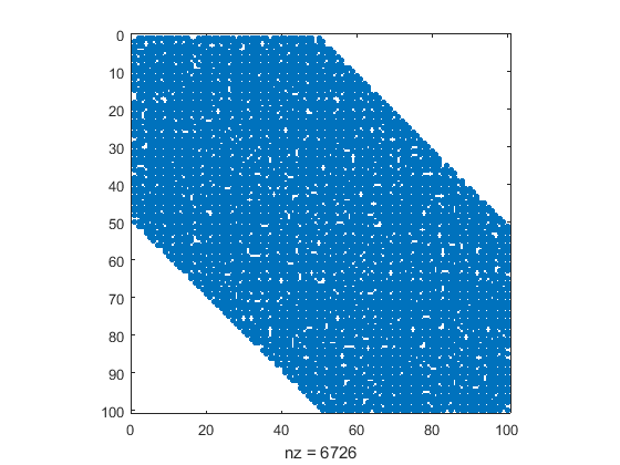
For the random linear graph in the last figure, the order in which the vertices appear makes its linear structure clear, and this is reflected in the band structure of its adjacency matrix. For large matrices with unknown ordering it might be a challenge to reveal its correct linear structure, as Figure 2.3 shows.

Figure 2.3. Random matrix before and after an appropriate permutation.

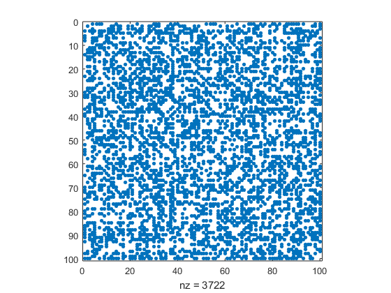
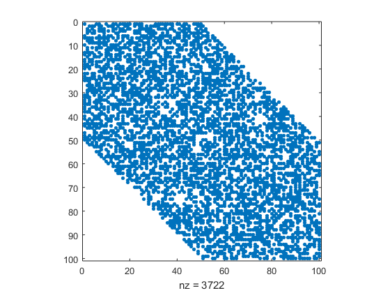
Now we can formulate the problem of reconstructing the linear embedding of the random graph as follows. Given a graph produced by a linear random graph model, find its linear embedding, or equivalently, retrieve the linear order of the vertices.

The model graph is a unit interval graph. It is well-known that the linear order can be retrieved in polynomial time, see for example [4, 10, 11]. The random graph we consider can be seen as a random subgraph of this graph. Such a graph has a clear linear structure, but the linear ordering cannot be retrieved with the same methods.

In the particular graph we consider, the order of the vertices of the model graph can also be retrieved by looking at the degree of the vertices: the end vertices have degree $n/2$, and the degrees increase near the middle, with a maximum of $n-1$ for the center vertices.

The degree of a vertex in the random graph is the result of a large number of idenpendent trials with identical probability. Thus, one could try to estimate the position of the vertices in the random matrix by considering the degree (vertices from both ends can be distinguished by the number of common neighbours). With high probability, the degree of vertex $v_{i}$, is

$$(n/2+i-1)p+\mathcal{O}(\sqrt{n}\log n),\text{ for }i=1,\ldots,n/2,\text{ and }$$

$$(3n/2-i+1)p+O(\sqrt{n}\log n),\text{ for }i=n/2+1,\ldots,n.$$

Thus, most vertices will drift at most $O(\sqrt{n}\log n)$ positions from their correct position, and consequently the number of inverted pairs is $o(n^{2})$. However, one can expect a non-neglible portion of all pairs to have a drift of $\sqrt{n}$. In comparison, our method gives the correct ordering for all vertices, except a small fraction near the ends. Moreover, in our approach, we can provide precise bounds on the number of pairs out of order and on the distance of vertices from their correct positions. As we will see, the results exhibits a trade off between how far vertices are from their original position and how far they are from the end, and the total number of such incorrectly placed vertices.

It is also possible to use a Stochastic Block Model to approximate the model matrix $M$ with blocks of size $\sqrt{n}$, for example. But that again gives only an approximated ordering, where vertices that belong to the same block will be positioned anywhere within it.

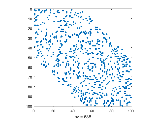
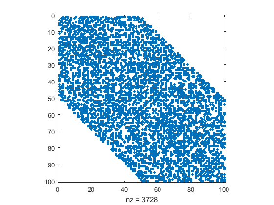
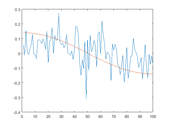
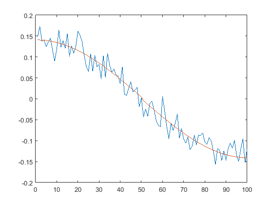
Before presenting an algorithm that retrieves the correct order we look at the eigenvectors of the matrices in question. We plot a specific eigenvector of the adjacency matrix by plotting the component values as a function of the indices. Figure 2.4 shows, for different probabilities $p$, the random matrix in the correct order and the eigenvector of the second largest eigenvalue.

$p=0.1$	$p=0.5$	$p=0.9$

Figure 2.4.

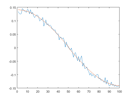The smooth curve in the graph of Figure 2.4 represents the eigenvector of the deterministic model matrix in the correct order. We will prove that the entries of this eigenvector are always monotonic for different matrix dimensions. Since its entries are monotonic, one could use it to find the correct embedding even when the matrix is given with the wrong order.

In Figure 2.4, the other line represents the entries of the eigenvector of the random matrix. Notice that the spiked lines exhibit the same decreasing trend as the straight lines. We will show that this is indeed true with high probability. That is, the corresponding eigenvector of the random matrix gives an order that is close to the correct order with high probability. Our first theorem shows that the second eigenvectors of random matrix and model matrix are close in norm.

Theorem 1.

Let $M$ be the linear graph model matrix with constant probability $p$ and variance $\sigma^{2}$, and let $\widehat{M}$ the random matrix following the model matrix. Let $x$ be a unitary eigenvector for $\lambda_{2}(M)$ and $\widehat{x}$ be an unitary eigenvector for $\lambda_{2}(\widehat{M})$. There is a constant $C_{0}>0$ such that

$$\left\|x-\widehat{x}\right\|\leq C_{0}n^{-1/2},$$

with probability at least $1-n^{-3}$.

Theorem 1 suggests the following algorithm to recover the order of a random linear graph.

Random matrix $\widehat{M}$

Compute $\widehat{x}$, the eigenvector for $\lambda_{2}(\widehat{M})$

Permute $\widehat{M}$ according to the order of the entries of $\widehat{x}$

return $\widehat{M}$

Algorithm 1 Order the adjacency matrix of the random linear graph

One important question that we are concerned with is the quality of the order provided by Algorithm 1. In particular, we want to know how many of such vertices exist and how far they are from their correct positions (see Section 5). We show that there is a trade off between how far vertices can be misplaced and the total amount of misplaced vertex pairs. In Section 5 we also calculate the rank correlation coefficients for the order provided by Algorithm 1.

A rank correlation coefficient measures the degree of similarity between two lists, and can be used to assess the significance of the relation between them. One can see the rank of one list as a permutation of the rank of the other. Statisticians have used a number of different measures of closeness for permutations. Some popular rank correlation statistics are Kendall’s $\tau$, Kendall distance, and Spearman’s footrule. There are several other metrics, and for different situations some metrics are preferable. For a deeper discussion on metrics on permutations we recommend [15].

In this paper, we will use the metrics defined as follows. The permutation $\sigma$ derived from an $n$-dimensional vector $y$ is the permutation obtained from ordering the components of $y$ in decreasing order. Specifically, we have that $y_{\sigma(1)}\geq y_{\sigma(2)}\geq\ldots\geq y_{\sigma(n)}$. When convenient we indicate it by $\sigma_{y}$.

To count the total number of inversions in $\sigma$ we use

$$D(\sigma)=\sum_{i<j}\textbf{1}_{\sigma(i)>\sigma(j)}\text{ (Kendall Distance)},$$

The distance that an element $i$ moved due to the permutation (the displacement or drift) is $\left|i-\sigma(i)\right|$. To count the total drift, we use

$$F(\sigma)=\sum_{i=1}^{n}|i-\sigma(i)|\text{ (Spearman's footrule)},$$

which is the total displacement of all elements. Finally, Kendall’s $\tau$ rank correlation coefficient is defined as

$$\tau=\frac{(\#concordant\ pairs-\#discordant\ pairs)}{\binom{n}{2}}=1-\frac{D(\sigma)}{n(n-1)}.$$

Even though metrics can be quite different from each other, in [14] Diaconis and Graham proved that Kendall distance and Spearman’s Footrule are equivalent measures in the following sense:

$$D(\sigma)\leq F(\sigma)\leq 2D(\sigma).$$

Thus, if the lists to be compared are large enough, these measures are of the same order. That is exactly our situation, where we want to quantify the number of vertices in the wrong order as $n$ tends to infinity.

Before providing metrics for the order given by the eigenvector of the random matrix, we need a better understanding of the displacement of vertices in that order. More precisely, we need to quantify how far vertices can be from the correct position and how many of them exists. In fact, we will see that this order is very accurate as the number of vertices grows.

To this end, we find an expression for the minimum distance between eigenvector $y$ of the random matrix and the known eigenvector $x$ of the model. We show that if there are too many incorrectly placed vertices, this lower bound is greater than the upper bound of Theorem 1. That means $y$ is too far from $x$, which happens with small probability. Therefore, the number of vertices in the wrong position can be quantified with high probability.

The next theorem reveals how the permutation of the eigenvector of the random matrix $\widehat{M}$ compares to the eigenvector of $M$. It says that large portions of vertices that are in the wrong order cannot be too far away from their correct positions, and entries that are too far represent a small group of vertices.

First we define a refined version of the Kendall distance. This version counts inverted pairs that appear after position $r$, and whose indices are at least $k$ positions apart. First note that, for a vector $y$, we can rewrite $D(\sigma_{y})$ as

(2.1) $$D(\sigma_{y})=|\{(i,j):y_{j}<y_{i}\mbox{ and }i<j\}|.$$

Given a vector $y$ and indices $k$ and $r$, let

$$D_{k,r}(y)=|\{(i,j):y_{j}<y_{i}\mbox{ and }i+k\leq j\mbox{ and }r\leq i\}|.$$

In particular, $D_{1,1}(y)=D(\sigma_{y})$. With this definition, the metric $D_{k,r}$ enables us to quantify inverted pairs locally inside specific ranges of the set $y$, while Kendall distance only provides a global measure. This way, it becomes more interesting for our purposes, as the next Theorem illustrates.

Theorem 2.

Let $y$ be the second eigenvector of the random matrix $\widehat{M}$. Let $r=n^{\alpha}$ and $k=n^{\beta}$. Then with probability $1-n^{-3}$ there is a constant $C>0$, such that if $\alpha\leq\beta$, then $D_{k,r}(y)<Cn^{5-2(\alpha+\beta)}$, and if $\alpha>\beta$, then $D_{k,r}(y)<Cn^{5-4\beta}$.

Here, whenever $\alpha+\beta>3/2$ and $\alpha\leq\beta$, or whenever $\beta>3/4$ and $\alpha<\beta$, we get the extremal cases where the number of inverted pairs satisfy $D_{k,r}(y)\in o(n^{2})$.

Theorem 3.

Let $y$ be the second eigenvector of the random matrix $\widehat{M}$, and let $k=n^{\beta}$. Then with probability $1-n^{-3}$ there is a constant $C>0$, such that $D_{k,1}(y)<Cn^{\frac{7-2\beta}{3}}$.

Now, if we take $\beta=1/2$, then $D_{k,1}\in o(n^{2})$, which means almost no vertex will drift more than $\sqrt{n}$ from its correct position. That ressembles the degree approach explained above, where the position of most vertices will drift at most $O(\sqrt{n}\log n)$ positions from their correct position.

Theorems 2 and 3 expose an interesting behavior in the group of bad vertices. There is a trade off between how far vertices can jump and the total number of such incorrectly placed vertices. That is useful for our purpose to establish metrics on the correctness of the rank. The next Theorem shows that the permutation derived from the second eigenvector $\hat{x}$ of the random matrix $\widehat{M}$ is well behaved.

Theorem 4.

Let $y$ be the second eigenvector of the random matrix $\widehat{M}$. Then $D(\sigma_{y})=\mathcal{O}(n^{9/5})$ with probability $1-n^{-3}$.

As a consequence, Kendall $\tau$ rank correlation coefficient is

Corollary 5.

$\tau=1-\mathcal{O}(n^{-1/5})$ with probability $1-n^{-3}$.

To prove Theorem 1 and quantify the error in the order given by Algorithm 1, our technique strongly relies on analytic expressions for the eigenvalues and eigenvectors of the model matrix. To this end, the next section provides the necessary information about the spectrum of the model matrix. One of the outcomes of Section 3 is that one eigenvector of the model matrix is steep enough. That means it contains the desired information about the structure of the graph, and provides the correct order of vertices. Moreover, consecutive entries differ significantly enough so that a small perturbation will have limited effect on the order. Further, in Section 4 we show that this steep eigenvector is close in norm to the eigenvector of the random graph. Thus, we prove Theorem 1 in Section 4. In Section 5 we perform a qualitative analysis of the problem and prove Theorems 2 and 4.

3. The eigenvalues of the model matrix

In this section we look to the spectrum of the model matrix which we identify by $M$. Consider the band matrix of even order $n$ defined as

$$A:=\left[\begin{array}[]{cccccccc}1&1&\ldots&1&0&0&\ldots&0\\ 1&1&&&1&&&0\\ \vdots&\vdots&\ddots&&&\ddots&&\vdots\\ 1&1&&&&&1&0\\ 0&1&&&&&&1\\ 0&&\ddots&&&&&1\\ \vdots&&&&&&&\vdots\\ 0&0&\ldots&0&1&1&\ldots&1\end{array}\right],$$

where exactly $s:=n/2$ columns have the first entry equal to $1$. Notice that $M=p(A-I)$. Thus $M$ and $A$ share the same eigenvectors with eigenvalues related as $\lambda(M)=p(\lambda(A)-1)$. For simplicity we proceed investigating the spectrum of $A$.

This matrix is an example of the familiar Toeplitz matrix which arises in many applications. Though Toeplitz matrices are well studied, their spectrum is unknown in the general form [6, 18]. Finding the spectrum seems to be a hard problem. There have been some advances in finding analytic expressions for the spectrum of particular instances, but to the best of our knowledge the spectrum of the matrix $A$ is unknown. In this section we find expressions for the $s$ eigenvalues and eigenvectors of $A$. Among them we identify the second largest, in absolute value, which is the main tool in this paper. We also characterize the remaining eigenvalues of $A$, and approximate its largest eigenvalue. We will need this information to bound the error between eigenvectors of model matrix and random matrix.

To this end, label the eigenvalues of $A$ as

$$\left|\lambda_{1}\left(A\right)\right|\geq\left|\lambda_{2}\left(A\right)\right|\geq\ldots\geq\left|\lambda_{n}\left(A\right)\right|.$$

In this section we prove the following result, which shows that the entries of the second eigenvector of the model matrix are monotonic.

Theorem 6.

The eigenvalue $\left|\lambda_{2}\left(A\right)\right|=1/\sqrt{2+2\cos\left(\frac{2s\pi}{2s+1}\right)}$ with corresponding eigenvector $u=\left[u_{j}\right]$ where $u_{j}=\cos\left(\frac{(2j-1)\pi}{4s+2}\right)$, for $j=1,\ldots,s$ and $u_{j}=-u_{n-j+1}$, for $j=s+1,\ldots,n$, where $s=n/2$.

In order to prove Theorem 6 we need to compute the eigenvalues of auxiliary matrices. Let $J$ be the matrix with all entries equal to $1$ and let $B:=J-A$. Then $B$ can be written in the form

$$B:=\left[\begin{array}[]{cccccccc}0&0&\ldots&0&1&1&\ldots&1\\ 0&0&&&0&&&1\\ \vdots&\vdots&\ddots&&&\ddots&&\vdots\\ 0&0&&&&&0&1\\ 1&0&&&&&&0\\ 1&&\ddots&&&&&0\\ \vdots&&&&&&&\vdots\\ 1&1&\ldots&1&0&0&\ldots&0\end{array}\right]=\left[\begin{array}[]{cc}&C^{T}\\ C\end{array}\right],\text{ where }C:=\left[\begin{array}[]{cccc}1&0&\cdots&0\\ 1&1&&\vdots\\ \vdots&&\ddots&0\\ 1&\ldots&1&1\end{array}\right]$$

is the lower triangular matrix of order $s=n/2$. Define the permutation matrix

$$P:=\left[\begin{array}[]{cccc}&&&1\\ &&1\\ &1\\ 1\end{array}\right].$$

Lemma 7.

Let $x$ be any eigenvector for the matrix $CP$ with eigenvalue $\lambda.$ Define vectors $y:=\left[\begin{array}[]{cc}Px^{T}&-x^{T}\end{array}\right]^{T}$ and $z:=\left[\begin{array}[]{cc}Px^{T}&x^{T}\end{array}\right]^{T}$. Then $By=-\lambda y$ and $Bz=\lambda z$.

Proof.

Now for any eigenvector $x$ for the matrix $CP$ we have $CPx=\lambda x$ and $C^{T}x=\lambda Px$. Thus we obtain

$$By=\left[\begin{array}[]{c}-C^{T}x\\ CPx\end{array}\right]=\left[\begin{array}[]{c}-\lambda Px\\ \lambda x\end{array}\right]=-\lambda y.$$

In the same way we can see that $Bz=\lambda z$. This finishes the proof. ∎

In light of Lemma 7, it suffice to compute the eigenvalues of $CP$ in order to get the eigenvalues of $B$. The next lemma describes these eigenvalues and its eigenvectors.

Theorem 8.

For $k=1\ldots s$, the eigenvalues of $B$ are $\lambda_{k}=1/\sqrt{2+2\cos\left(\frac{2k\pi}{2s+1}\right)}$ with corresponding eigenvectors $u^{k}=\left[u_{j}\right]$ where $u_{j}=\left(-1\right)^{j}\sin\left(\frac{2jk\pi}{2s+1}\right)$, for $j=1,\ldots,s$ and $u_{j}=-u_{n-j+1}$, for $j=s+1,\ldots,n$.

For $k=s+1\ldots n$ we have $\lambda_{k}=-1/\sqrt{2+2\cos\left(\frac{2k\pi}{2s+1}\right)}$ with corresponding eigenvectors $u^{k}=\left[u_{j}\right]$ where $u_{j}=\left(-1\right)^{j}\sin\left(\frac{2jk\pi}{2s+1}\right)$, for $j=1,\ldots,s$ and $u_{j}=u_{n-j+1}$, for $j=s+1,\ldots,n$.

Proof.

We will show that for $k=1\ldots s$ the eigenvalues $\lambda_{k}$ of $CP$ are $1/\sqrt{2+2\cos\left(\frac{2k\pi}{2s+1}\right)}$ with corresponding eigenvectors $u^{k}=\left[u_{j}\right]$ where $u_{j}=\left(-1\right)^{j}\sin\left(\frac{2jk\pi}{2s+1}\right)$, for $j=1,\ldots,s$. Then, by Lemma 7 the proof is done.

We notice that

$$CP=\left[\begin{array}[]{cccc}0&\cdots&0&1\\ 0&&\iddots&\vdots\\ \vdots&1&&1\\ 1&\ldots&1&1\end{array}\right],\left(CP\right)^{2}=\left[\begin{array}[]{ccccc}1&1&\cdots&1&1\\ 1&2&&2&2\\ \vdots&&\ddots&\vdots&\vdots\\ 1&2&\cdots&s-1&s-1\\ 1&2&\cdots&s-1&s\end{array}\right]\text{, and }\left(CP\right)^{-2}=\left[\begin{array}[]{ccccc}2&-1\\ -1&2&-1\\ &-1&\ddots&\ddots\\ &&\ddots&2&-1\\ &&&-1&1\end{array}\right].$$

That is familiar tridiagonal matrix which appears often in the literature. One of the oldest works where its eigenvalues were reported is in [16]. We finish the proof by indicating that the tridiagonal matrix $\left(CP\right)^{-2}$ has eigenvalues $2+2\cos\left(\frac{2k\pi}{2s+1}\right)$ for $k=1\ldots s$, with corresponding eigenvector $u=\left[u_{j}\right]$ where $u_{j}=\left(-1\right)^{j}\sin\left(\frac{2jk\pi}{2s+1}\right)$, for $j=1,\ldots,s$. Thus, $u$ is an eigenvector for $CP$ with corresponding eigenvalue $\lambda_{k}=1/\sqrt{2+2\cos\left(\frac{2k\pi}{2s+1}\right)}$. This concludes the proof. ∎

Now, we are ready to prove the following theorem concerning the eigenvalues of $A$.

Theorem 9.

$\left|\lambda_{2}\left(A\right)\right|=\left|\gamma_{2}\right|$, where $\gamma_{2}$ is the second largest eigenvalue of $B$ in absolute value. Besides, both eigenvalues have the same eigenvector.

Proof.

First, we notice that all matrices $A,$ $B$ and $J$ satisfy the Perron-Frobenius Theorem. Therefore, they all have a unique eigenvector with entries of the same sign corresponding to the largest eigenvalue in absolute value. They are called Perron vector and Perron value for the matrix of interest. Next, we define the set $H$ which is just the set of unit vectors excluding all possible Perron vectors.

$$H:=\left\{x\in\mathbb{R}^{n}\backslash\left\{\mathbb{R}_{+}^{n}\cup\mathbb{R}_{-}^{n}\right\}:\left\|x\right\|=1\right\}.$$

The Perron value of $A$ can be expressed as

$$\left|\lambda_{1}(A)\right|=\max_{\left\|x\right\|=1}x^{T}Ax.$$

Thus, if we restrict the set of vectors where we take the maximum to the set $H$, we get

$$\left|\lambda_{2}(A)\right|=\max_{x\in H}\left|x^{T}Ax\right|.$$

And the same maximization problem can be used to identify $\left|\gamma_{2}\right|$ and $\left|\lambda_{2}(J)\right|$. Finally, we can write

$$\left|\lambda_{2}(A)\right| = \max_{x\in H}\left|x^{T}(J-B)x\right|$$

$$\leq \max_{x\in H}\left\{\left|x^{T}Jx\right|+\left|x^{T}Bx\right|\right\}$$

$$\leq \max_{x\in H}\left|x^{T}Jx\right|+\max_{x\in H}\left|x^{T}Bx\right|$$

$$= \left|\lambda_{2}(J)\right|+\left|\gamma_{2}\right|.$$

Besides, the only nonzero eigenvalue of $J$ is its Perron value. Therefore, the above inequality is simply

$$\left|\lambda_{2}(A)\right|\leq\left|\gamma_{2}\right|.$$

By noticing that $B=J-A$, the same calculation gives us the inequality $\left|\gamma_{2}\right|\leq\left|\lambda_{2}(A)\right|.$ Both inequalities prove the first statement of the theorem.

To see that $\lambda_{2}(A)$ and $\gamma_{2}$ have the same eigenvector we apply Theorem 8. According to this theorem, there is an eigenvector $u$ of $\gamma_{2}$, with positive and negative entries, such that $u=\left[\begin{array}[]{cc}Pv^{T}&-v^{T}\end{array}\right]^{T}$. Clearly $Ju=0$ and then

$$Au=(J-B)u=-Bu=-\gamma_{2}u.$$

That finishes the proof. ∎

Next, we prove the main theorem of this section.

Proof.

(Theorem 6) Now the proof of Theorem 6 follows easily from Theorem 8 and Theorem 9. The largest eigenvalue of $B$ occurs for $k=1$ in Theorem 8. Relabelling the eigenvalues $\lambda_{i}(B)$ for $i=1\ldots n$ such that$\left|\gamma_{1}\right|\geq\left|\gamma_{2}\right|\geq\ldots\geq\left|\gamma_{n}\right|$, we see that $\left|\gamma_{1}\right|=\left|\gamma_{2}\right|$. Consider $k=1$ in Theorem 8. The entries of the eigenvector of $\lambda_{1}(A)$ can be rewritten as $u_{j}=\cos\left(\frac{(2j-1)\pi}{4s+2}\right)$, for $j=1,\ldots,s$, and that establishes Theorem 6. ∎

4. The eigenvectors of the random graph

We apply random matrix theory and the results about the spectrum of the model matrix, obtained above, to show that the second eigenvector of the random graph is, with high probability, close to the second eigenvector of the model. Thus the second eigenvector of the random matrix can be used to reveal the correct linear structure of the random graph.

In the last few years, there has been significant progress on the subject of random matrices, especially around the universality phenomenon [23] and concentration inequalities (see [24, 26] for good surveys). For our purposes, we will use the following concentration inequality from [27].

Lemma 10.

(Norm of a random matrix). There is a constant $C>0$ such that the following holds. Let $E$ be a symmetric matrix whose upper diagonal entries $e_{ij}$ are independent random variables where $e_{ij}=1-p_{ij}$ or $-p_{ij}$ with probabilities $p_{ij}$ and $1-p_{ij}$ , respectively, where $0\leq p_{ij}\leq 1$. Let $\sigma^{2}=\max_{ij}p_{ij}(1-p_{ij})$. If $\sigma^{2}\geq C\log n/n$, then

$$\mathbb{P}(\left\|E\right\|\geq C\sigma n^{1/2})\leq n^{-3}.$$

A well-known result by Davis and Kahan [12], from matrix theory says that the angle between eigenvectors of the model matrix and of the random one is bounded in terms of their spectrum:

Lemma 11.

(Davis-Kahan) Let $A$ and $\widehat{A}$ be symmetric matrices, $\lambda_{i}$ be the $i-$th largest eigenvalue of $A$ with eigenvector $x_{i}$, and $\widehat{x_{i}}$ be the eigenvector of the $i-$th largest eigenvalue of $\widehat{A}$. If $\theta$ is the angle between $x_{i}$ and $\widehat{x_{i}}$, then

$$\sin 2\theta\leq\frac{2\left\|A-\widehat{A}\right\|}{\min_{i\neq j}\left|\lambda_{i}-\lambda_{j}\right|},\text{ provided }\lambda_{i}\neq\lambda_{j}.$$

To apply the Davis-Kahan Theorem to $\lambda_{2}$, we need the smallest gap between the eigenvalues. The next Theorem helps us with that.

Theorem 12.

$\lambda_{1}(A)=1/\sqrt{2-2\cos\left(\theta_{1}\right)}$, where $\theta_{1}\leq\frac{\pi}{4s}$ and $\lambda_{3}(A)=1/\sqrt{2-2\cos\left(\theta_{3}\right)}$, where $\theta_{3}>\frac{\pi}{s}$.

To prove Theorem 12 and characterize the additional eigenvalues of $A$ we consider the following matrix

$$D=\left[\begin{array}[]{ccccc}1&\cdots&&1&1\\ 1&&&\iddots&2\\ &&&\iddots&\vdots\\ \vdots&1&&2&2\\ 1&2&\ldots&2&2\end{array}\right].$$

Lemma 13.

Let $x$ be any eigenvector for matrix $D$ with eigenvalue $\lambda.$ Define the vector $y:=\left[\begin{array}[]{cc}x^{T}&Px^{T}\end{array}\right]^{T}$. Then $Ay=\lambda y$.

Proof.

First, we have $A\left[\begin{array}[]{c}I\\ P\end{array}\right]=\left[\begin{array}[]{cc}J&C\\ C^{T}&J\end{array}\right]\left[\begin{array}[]{c}I\\ P\end{array}\right]=\left[\begin{array}[]{c}J+CP\\ C^{T}+JP\end{array}\right]=\left[\begin{array}[]{c}D\\ PD\end{array}\right].$ Then $Ay=A\left[\begin{array}[]{c}I\\ P\end{array}\right]x=\left[\begin{array}[]{c}D\\ PD\end{array}\right]x=\lambda\left[\begin{array}[]{c}x\\ Px\end{array}\right]=\lambda y.$

∎

The previous lemma leads us to the study of the spectrum of the matrix $D$.

Theorem 14.

Let $D$ be as defined above, of even order $s$. Then, its eigenvalues are $\lambda_{k}=1/\sqrt{2-2\cos\left(\theta_{k}\right)}$, for $k=1\ldots s$, where $\theta_{k}$ is a root of the equation

$$p(\theta)=\sin\left(\left(s+1\right)\theta\right)+3\sin\left(s\theta\right)-4\sin\left(\left(s-1\right)\theta\right)-4\sin\left(\theta\right).$$

Proof.

It is easy to verify that

$$D^{-1}=\left[\begin{array}[]{ccccc}2&0&\cdots&&-1\\ 0&&&-1&1\\ \vdots&&\iddots&\iddots&0\\ &&&&\vdots\\ -1&1&0&\cdots&0\end{array}\right]\text{ and }D^{-2}=\left[\begin{array}[]{ccccc}5&-1&&&-2\\ -1&2&-1\\ &-1&\ddots&\ddots\\ &&\ddots&2&-1\\ -2&&&-1&2\end{array}\right].$$

Therefore, it suffices to prove that the eigenvalues of $D^{-2}$ are of the required form $2-2\cos\left(\theta\right)$.

In order to do that, we obtain an expression for the characteristic polynomial of $D^{-2}$. A relevant matrix related to this expression is the order $s$ matrix defined as

$$E_{s}=\left[\begin{array}[]{ccccc}2-\lambda&-1&0&\cdots&0\\ -1&2-\lambda&&\ddots&\vdots\\ 0&&&&0\\ \vdots&\ddots&&\ddots&-1\\ 0&\cdots&0&-1&2-\lambda\end{array}\right].$$

Below $\left|M\right|_{n}$ indicates the determinant of the order $n$ matrix $M$. By expanding the first row the determinant of $D^{-2}-\lambda I$, we can write

$$det(D^{-2}-\lambda I) = (5-\lambda)\left|E_{s-1}\right|$$

$$-\left|\begin{array}[]{ccccc}-1&-1&0&\cdots&0\\ 0&2-\lambda&-1&0\\ \vdots&-1&\ddots&\ddots\\ 0&&\ddots&&-1\\ -2&0&\cdots&-1&2-\lambda\end{array}\right|_{s-1}+2\left|\begin{array}[]{ccccc}-1&2-\lambda&-1&&0\\ 0&-1&2-\lambda&\ddots\\ \vdots&0&\ddots&\ddots&-1\\ 0&&\ddots&-1&2-\lambda\\ -2&0&\cdots&0&-1\end{array}\right|_{s-1}.$$

Then we expand the second and third determinants by the first column, which gives us

$$det(D^{-2}-\lambda I) = (5-\lambda)\left|E_{s-1}\right|$$

$$-\left(\left|E_{s-2}\right|+2\left|\begin{array}[]{ccccc}-1&0&\cdots&&0\\ 2-\lambda&-1&0&&0\\ -1&\ddots&\ddots&\ddots&\vdots\\ &\ddots&&&0\\ 0&&-1&2-\lambda&-1\end{array}\right|_{s-2}\right)$$

$$+2\left(-\left|\begin{array}[]{ccccc}-1&2-\lambda&-1&&0\\ 0&-1&2-\lambda&\ddots\\ &0&\ddots&\ddots\\ &&\ddots\\ &&\ddots&-1&2-\lambda\\ 0&&\cdots&0&-1\end{array}\right|_{s-2}-2\left|E_{s-2}\right|\right)$$

$$= (5-x)\left|E_{s-1}\right|-5\left|E_{s-2}\right|.$$

$$-4\left|\begin{array}[]{ccccc}-1&2-\lambda&-1&&0\\ 0&-1&2-\lambda&\ddots\\ &0&\ddots&\ddots\\ &&\ddots\\ &&\ddots&-1&2-\lambda\\ 0&&\cdots&0&-1\end{array}\right|_{s-2}$$

Since the last matrix has even order and $-1$ in the diagonal, we get

(4.5) $$det(D^{-2}-\lambda I)=(5-\lambda)\left|E_{s-1}\right|-5\left|E_{s-2}\right|-4.$$

From this point, we call up Chebyshev polynomials of second kind. They are defined by the recurrence relation

$$U_{0}(x) =1$$

$$U_{1}(x) =2x$$

$$U_{n+1}(x) =2xU_{n}(x)-U_{n-1}(x).$$

Besides, it is a well-known fact that $U_{n}(x)$ obeys the determinant identity

$$U_{n}(x)=\left|\begin{array}[]{cccc}2x&-1&0&0\\ -1&2x&\ddots&0\\ 0&\ddots&\ddots&-1\\ 0&0&-1&2x\end{array}\right|_{n}.$$

Therefore, a change of variable $x=\frac{2-\lambda}{2}$ provides us the determinant

$$\left|E_{s}\right|=U_{s}\left(\frac{2-\lambda}{2}\right)$$

and the relation

$$U_{s+1}\left(\frac{2-\lambda}{2}\right)=\left(2-\lambda\right)U_{s}\left(\frac{2-\lambda}{2}\right)-U_{s-1}\left(\frac{2-\lambda}{2}\right),$$

which we apply in the equivalent form

$$\left(2-\lambda\right)U_{s}\left(\frac{2-\lambda}{2}\right)=U_{s+1}\left(\frac{2-\lambda}{2}\right)+U_{s-1}\left(\frac{2-\lambda}{2}\right).$$

In this manner, equation (4.5) becomes

$$det(D^{-2}-\lambda I) = (3+2-\lambda)U_{s-1}\left(\frac{2-\lambda}{2}\right)-5U_{s-2}\left(\frac{2-\lambda}{2}\right)-4$$

$$= U_{s}\left(\frac{2-\lambda}{2}\right)+3U_{s-1}\left(\frac{2-\lambda}{2}\right)-4U_{s-2}\left(\frac{2-\lambda}{2}\right)-4.$$

Furthermore, one of many well-known properties of Chebyshev polynomials is

$$U_{n}(cos\theta)=\frac{\sin\left(\left(n+1\right)\theta\right)}{\sin\theta}.$$

Therefore, the change of variables $\cos\theta=\frac{2-\lambda}{2}$ allows us to rewrite $det(D^{-2}-\lambda I)$ as

$$det(D^{-2}-(2-2\cos\theta)I)=\frac{\sin\left(\left(s+1\right)\theta\right)+3\sin\left(s\theta\right)-4\sin\left(\left(s-1\right)\theta\right)-4\sin\left(\theta\right)}{\sin\left(\theta\right)}.$$

Finally, $2-2\cos\theta$ is an eigenvalue of $D^{-2}$ whenever $\theta$ is a root of the equation

$$p(\theta)=\sin\left(\left(s+1\right)\theta\right)+3\sin\left(s\theta\right)-4\sin\left(\left(s-1\right)\theta\right)-4\sin\left(\theta\right),$$

which concludes the proof.∎

Theorem 15.

Let $D$ be a matrix as defined earlier, of even order $s\geq 5$. Then, its largest eigenvalues

$$\lambda_{i}=1/\sqrt{2-2\cos\left(\theta_{i}\right)},$$

for $i=1,2$ are such that $\theta_{1}\in\left(\frac{\pi}{s^{2}},\frac{\pi}{4s}\right)$ and $\theta_{2}>\frac{\pi}{s}$.

Proof.

To bound $\theta_{1}$, Theorem 14 guarantees it is enough to locate the smallest root of

$$p(\theta)=\sin\left(\left(s+1\right)\theta\right)+3\sin\left(s\theta\right)-4\sin\left(\left(s-1\right)\theta\right)-4\sin\left(\theta\right).$$

On one hand, by means of trigonometric identities we get

$$p\left(\frac{x\pi}{s}\right)=-3\,\sin\left(x\pi\right)\cos\left({\frac{x\pi}{s}}\right)+5\,\cos\left(x\pi\right)\sin\left({\frac{x\pi}{s}}\right)+3\,\sin\left(x\pi\right)-4\,\sin\left({\frac{x\pi}{s}}\right).$$

We claim that $p\left(\frac{x\pi}{s}\right)<0$ for $x\in[1/4,1)$. To see it, it is enough to show that

$${\frac{5\,\cos\left(x\pi\right)-4}{3\sin\left(x\pi\right)}}<\frac{\cos\left(\frac{x\pi}{s}\right)-1}{\sin\left(\frac{x\pi}{s}\right)},$$

for $x\in[1/4,1)$. Notice that $\frac{5\,\cos\left(x\pi\right)-4}{3\sin\left(x\pi\right)}$ is a decreasing function in $x$ for $x\in[1/4,1)$. Thus, it is enough to show that

$${\frac{5\,\cos\left(\pi/4\right)-4}{3\sin\left(\pi/4\right)}}<\frac{\cos\left(\frac{x\pi}{s}\right)-1}{\sin\left(\frac{x\pi}{s}\right)}.$$

Also $\frac{\cos\left(x\frac{\pi}{s}\right)-1}{\sin\left(x\frac{\pi}{s}\right)}$ is an decreasing function in $x$ for $x\in[1/4,1]$ and increasing as a function in $s$. Thus, it is enough to check that

$${\frac{5\,\cos\left(\pi/4\right)-4}{3\sin\left(\pi/4\right)}}<\frac{\cos\left(\frac{\pi}{s}\right)-1}{\sin\left(\frac{\pi}{s}\right)}.$$

In fact, the inequality is true for $s\geq 2$, thus the claim follows.

On the other hand, the Taylor series of $p\left(\theta\right)$ at $\theta=0$ is

$$\theta+\left(-\frac{5}{2}\,s^{2}+\frac{3}{2}\,s-\frac{1}{6}\right)\theta^{3}+\left({\frac{5}{24}}\,{s}^{4}-\frac{1}{4}\,{s}^{3}+{\frac{5}{12}}\,{s}^{2}-\frac{1}{8}\,s+{\frac{1}{120}}\right){\theta}^{5}+\mathcal{O}\left({\theta}^{6}\right).$$

Furthermore, if $s$ is not too small the terms of order 5 or greater adds up to a positive constant, thus

$$f(\theta)=\theta+\left(-\frac{5}{2}\,s^{2}+\frac{3}{2}\,s-\frac{1}{6}\right)\theta^{3}\leq p\left(\theta\right)$$

and

$$f\left(\frac{\pi}{s^{2}}\right)=\frac{\pi\left(6s^{4}-15\pi^{2}s^{2}+9\pi^{2}s-\pi^{2}\right)}{6s^{6}}.$$

Now, the polynomial $6s^{4}-15\pi^{2}s^{2}+9\pi^{2}s-\pi^{2}$ in the variable $s$ has largest root smaller than $5$. Therefore,

$$0\leq f\left(\frac{\pi}{s^{2}}\right)\leq p\left(\frac{\pi}{s^{2}}\right)\text{ and }p\left(\frac{\pi}{4s}\right)<0.$$

Then, by continuity $p\left(\theta\right)$ has a root in $\left(\frac{\pi}{s^{2}},\frac{\pi}{4s}\right)$. Finally, the fact that $p\left(\frac{x\pi}{s}\right)<0$ for $x\in[1/4,1)$ guarantees that $\theta_{2}>\frac{\pi}{s}$, which concludes the proof. ∎

Finally, we are able to look at $\lambda_{1}(A)$ and $\lambda_{3}(A)$ and prove Theorem 12.

Proof.

(Theorem 12) By Lemma 13, each eigenvalue of $D$ is an eigenvalue of $A$. Thus, by Theorem 15 the proof is done for $\lambda_{1}$ if we prove that $\lambda_{1}(A)=\lambda_{1}(D)$. But that is easy to see, since $D$ and $A$ are matrices that fulfill Perron-Frobenius Theorem. Thus, its unique largest eigenvalue has an eigenvector with entries of the same sign, so called Perron vector. Again by Lemma 13, if $x$ is a Perron vector of $D$, then $\left[\begin{array}[]{cc}x^{T}&Px^{T}\end{array}\right]^{T}$ is an eigenvector of $A$ with entries of the same sign. Thus it must be a Perron vector of $A$, which gives us $\lambda_{1}(A)=\lambda_{1}(D)$.

Now $\lambda_{3}(A)$ is characterized by Lemma 13, which provides the eigenvalues with odd indices for $A$, and Theorem 15. Thus $\lambda_{3}(A)=1/\sqrt{2-2\cos\left(\theta_{3}\right)}$, where $\theta_{3}>\frac{\pi}{s}$. That finishes the proof. ∎

Finally, the results of this section enables us to prove Theorem 1.

Proof.

(Theorem 1) We can view the adjacency matrix $\widehat{M}$ as a perturbation of $M$, $\widehat{M}=M+E$, where the entries of $E$ are $e_{ij}=1-p$ with probability $p$ and $-p$ with probability $1-p$. That way $E$ is as in Lemma 10, and then with probability at least $1-n^{-3}$, we have

(4.6) $$\left\|E\right\|\leq C\sigma\sqrt{n},$$

for some constant $C>0$. Since $x$ and $\widehat{x}$ are both unitary we have $\left\|x-\widehat{x}\right\|\leq\sqrt{2}\sin\theta$, where $\theta$ is the angle they form. Therefore, we can apply Lemma 11 and equation (4.6), to obtain a constant $C_{1}>0$ such that

(4.7) $$\left\|x-\widehat{x}\right\| \leq \frac{C_{1}\left\|M-\widehat{M}\right\|}{\min_{i\neq 2}\left|\lambda_{i}-\lambda_{2}\right|},$$

$$\leq \frac{C_{1}\sigma\sqrt{n}}{\min_{i\neq 2}\left|\lambda_{i}-\lambda_{2}\right|}.$$

Also, if $A$ is as in Theorem 6, we have $M=p(A-I).$ Now, to bound the gap between the eigenvalues, we apply Theorems 6 and 12, to get

$$\lambda_{1}(M)=p\lambda_{1}(A-I)=p/\sqrt{2-2\cos\left(t_{1}\right)}-p,$$

$$\lambda_{3}(M)=p\lambda_{3}(A-I)=p/\sqrt{2-2\cos\left(t_{3}\right)}-p\text{ and}$$

$$\lambda_{2}(M)=p\lambda_{2}(A-I)=p/\sqrt{2+2\cos\left(\frac{2s\pi}{2s+1}\right)}-p,$$

where $t_{1}\leq\frac{\pi}{4s}$, $t_{3}>\frac{\pi}{s}$, and $s=\frac{n}{2}$ . Notice that, since $\cos\left(\theta_{1}\right)$ is decreasing in $\theta_{1}$, we have

$$\frac{1}{\lambda_{1}-\lambda_{2}}\leq\frac{1}{p/\sqrt{2-2\cos\left(\frac{\pi}{4s}\right)}-p/\sqrt{2+2\cos\left(\frac{2s\pi}{2s+1}\right)}}.$$

Now, an asymptotic expansion of the last expression, shows that there is a constant $B_{1}>0$ such that

$$\frac{1}{\lambda_{1}-\lambda_{2}}\leq\frac{B_{1}}{s}.$$

Similarly, we obtain a constant $B_{2}>0$ such that

$$\frac{1}{\lambda_{3}-\lambda_{1}}\leq\frac{B_{2}}{s}.$$

Therefore, for some constant $C_{2}>0$ inequality 4.7 becomes

$$\left\|x-\widehat{x}\right\|\leq\frac{C_{2}\sqrt{n}}{s}=\frac{2C_{2}\sqrt{n}}{n}.$$

That finishes the proof. ∎

5. Bounding the number of misplaced vertices

Our method relies on the asymptotic expansions of the terms $x_{i}$ regarding it as a function of $n$, as the next Lemma states.

Lemma 16.

Let $x$ be the unitary eigenvector for $\lambda_{2}\left(A\right)$. Then

$$\left(x_{r}-x_{r+k}\right)^{2}=\frac{1}{\pi}\,k^{2}\left(2\,r+k-1\right)^{2}\theta^{5}+O\left(\theta^{7}\right),$$

where $\theta=\frac{\pi}{2s+1}$.

Proof.

Theorem 6 provides the expressions we need to compute $x_{j}$: we have $x_{j}=\omega\cos\left(\frac{(2j-1)\pi}{4s+2}\right)$, for $j=1,\ldots,s$, where $\omega$ is a constant such that $\left\|x\right\|=1$. Thus,

$$\left(x_{r}-x_{r+k}\right)^{2}=\omega^{2}\left(\cos\left(\frac{(2r-1)\pi}{4s+2}\right)-\cos\left(\frac{(2(r+k)-1)\pi}{4s+2}\right)\right)^{2}.$$

To find $\omega^{2}$, we make use of the trigonometric identity

$$\sum_{i=0}^{k-1}\cos(2\alpha i+\beta)=\frac{\sin\left(k\alpha\right)\cos\left(\beta+\left(k-1\right)\alpha\right)}{\sin\alpha}.$$

Then, we can write

(5.1) $$c = \sum_{i=1}^{s}\cos^{2}\left(\frac{(2i-1)\pi}{4s+2}\right)$$

$$= \sum_{i=0}^{s-1}\cos^{2}\left((2i+1)\frac{\pi}{4s+2}\right)$$

$$= \frac{1}{2}\sum_{i=0}^{s-1}\left(1+\cos\left(2(2i+1)\frac{\pi}{4s+2}\right)\right)$$

$$= \frac{s}{2}+\frac{\sin\left(\frac{s\pi}{2s+1}\right)\cos\left(\frac{s\pi}{2s+1}\right)}{2\sin\left(\frac{\pi}{2s+1}\right)}.$$

Setting $\theta=\frac{\pi}{2s+1}$, we get $s=\frac{\pi}{2\theta}-\frac{1}{2}$ and then

$$\cos\left(\frac{s\pi}{2s+1}\right)=\sin\left(\frac{\theta}{2}\right)\text{ and }\sin\left(\frac{s\pi}{2s+1}\right)=\cos\left(\frac{\theta}{2}\right).$$

Therefore, by means of trigonometric identities, we obtain $c=\pi/4\theta$. Thus

(5.2) $$\omega^{2}=\frac{1}{c}=\frac{4\theta}{\pi}.$$

On the other hand, the Taylor series for $\left(\cos\left(\frac{(2r-1)\theta}{2}\right)-\cos\left(\frac{(2(r+k)-1)\theta}{2}\right)\right)^{2}$ is given by

$$\frac{1}{4}\,k^{2}\left(2\,r+k-1\right)^{2}\theta^{4}+O\left(\theta^{6}\right).$$

Therefore,

$$\left(x_{r}-x_{r+k}\right)^{2}=\frac{1}{\pi}\,k^{2}\left(2\,r+k-1\right)^{2}\theta^{5}+O\left(\theta^{7}\right),$$

as required ∎

The last result enables us to prove the main Theorems of this section.

Proof.

(Theorem 2) Recall that in our notation $x_{1}>x_{2}>\ldots>x_{s}$. Fix $r=n^{\alpha}$ and $k=n^{\beta}$, and let

$$R=\{(i,j):y_{j}<y_{i}\mbox{ and }i+k\leq j\mbox{ and }r\leq i\}.$$

Then

$$2n\|x-y\|^{2}=\sum_{i=1}^{n}\sum_{j=1}^{n}(x_{i}-y_{i})^{2}+(x_{j}-y_{j})^{2}\geq\sum_{(i,j)\in R}(x_{i}-y_{i})^{2}+(x_{j}-y_{j})^{2}.$$

Since $y_{j}\geq y_{i}$ and $x_{j}<x_{i}$, the minimum contribution that each term in the sum can provide happens when

$$y_{i}=y_{j}=\frac{x_{i}+x_{j}}{2}.$$

Thus, we have

$$2n\left\|x-y\right\|^{2}>\sum_{(i,j)\in R}\left(x_{i}-\frac{x_{i}+x_{j}}{2}\right)^{2}+\left(x_{j}-\frac{x_{i}+x_{j}}{2}\right)^{2}=\sum_{(i,j)\in R}\frac{\left(x_{i}-x_{j}\right)^{2}}{2}.$$

Besides $i+k\geq j$, and then the last expression is minimum for $j=i+k$. Then we can write

$$2n\left\|x-y\right\|^{2}>\sum_{(i,j)\in R}\frac{\left(x_{i}-x_{i+k}\right)^{2}}{2}.$$

By Lemma 16, for $n$ large enough

$$2n\left\|x-y\right\|^{2}>\frac{1}{2\pi}\sum_{(i,j)\in R}\frac{k^{2}\left(2\,i+k-1\right)^{2}}{n^{5}}>\frac{k^{2}}{2\pi n^{5}}\sum_{(i,j)R}i^{2}+k^{2}.$$

By definition $r\leq i$. For $r=n^{\alpha}$ and $k=n^{\beta}$, we can write

$$2n\left\|x-y\right\|^{2}>\frac{n^{2\beta}}{2\pi n^{5}}\sum_{(i,j)R}n^{2\alpha}+n^{2\beta}.$$

That gives the bound

$$2n\left\|x-y\right\|^{2}>C_{1}\frac{n^{2\beta}}{n^{5}}|R|(n^{2\alpha}+n^{2\beta}),$$

for an absolute constant $C_{1}>0$. Equivalently, we get

$$\left\|x-y\right\|^{2}>C_{1}|R|(n^{2(\alpha+\beta)-6}+n^{4\beta-6}).$$

On the other hand, by Theorem 1 there is a constant $C_{0}>0$ such that with probability $1-n^{-3}$

$$\left\|x-y\right\|^{2}\leq C_{0}n^{-1}.$$

Combining these two inequalities, we obtain a constant $C_{2}>0$ such that

$$|R|<C_{2}(n^{5-2(\alpha+\beta)}+n^{5-4\beta}).$$

with probability $1-n^{-3}$. That finishes the proof. ∎

Proof.

(Theorem 3) Recall that in our notation $x_{1}>x_{2}>\ldots>x_{s}$. Fix $k=n^{\beta}$, and let

$$R=D_{k,1}=\{(i,j):y_{j}<y_{i}\mbox{ and }i+k\leq j\}.$$

Then

$$2n\|x-y\|^{2}=\sum_{i=1}^{n}\sum_{j=1}^{n}(x_{i}-y_{i})^{2}+(x_{j}-y_{j})^{2}\geq\sum_{(i,j)\in R}(x_{i}-y_{i})^{2}+(x_{j}-y_{j})^{2}.$$

Since $y_{j}\geq y_{i}$ and $x_{j}<x_{i}$, the minimum contribution that each term in the sum can provide happens when

$$y_{i}=y_{j}=\frac{x_{i}+x_{j}}{2}.$$

Thus, we have

(5.3) $$2n\left\|x-y\right\|^{2}>\sum_{(i,j)\in R}\left(x_{i}-\frac{x_{i}+x_{j}}{2}\right)^{2}+\left(x_{j}-\frac{x_{i}+x_{j}}{2}\right)^{2}=\sum_{(i,j)\in R}\frac{\left(x_{i}-x_{j}\right)^{2}}{2}.$$

If there are $n_{i}$ pairs $(i,j)$, then we can index $j$’s as $(i,j_{i_{1}}),\dots(i,j_{i_{n_{i}}}),\text{ for }i=1,\ldots,n.$ Here, the total number of inverted pairs is $\sum_{i=1}^{n}n_{i}=|R|$. Furthermore, for a fixed $i$ the we obtain the minimum $(x_{i}-x_{j})^{2}$ whenever $j-i$ is minimum. Therefore, since $i+k\leq j$ for each $i$ the minimum sum

$$\sum_{t=1}^{n_{i}}\left(x_{i}-x_{j_{i_{t}}}\right)^{2}$$

occurs whenever $j_{i_{1}}=i+k,j_{i_{2}}=i+k+1,\dots,j_{i_{n_{i}}}=i+k+n_{i}-1$. Therefore, inequality (5.3) becomes

$$2n\left\|x-y\right\|^{2}>\sum_{i=1}^{n}\sum_{t=0}^{n_{i}-1}\frac{\left(x_{i}-x_{i+k+t}\right)^{2}}{2}.$$

By Lemma 16, for $n$ large enough

$$2n\left\|x-y\right\|^{2}>\frac{1}{2\pi}\sum_{i=1}^{n}\sum_{t=0}^{n_{i}-1}\frac{(k+t)^{2}(i+k+t)^{2}}{n^{5}}>\frac{k^{2}}{2\pi n^{5}}\sum_{i=1}^{n}\sum_{t=0}^{n_{i}-1}t^{2}.$$

Therefore, for $n$ large enough there is a constant $C_{1}>0$ such that

(5.4) $$2n\left\|x-y\right\|^{2}>C_{1}k^{2}\sum_{i=1}^{n}n_{i}^{3}.$$

Recall that two $p$-norms are related by $\left\|x\right\|_{p}\leq n^{\frac{1}{p}-\frac{1}{q}}\left\|x\right\|_{q}$. Taking $p=1$ and $q=3$, we obtain that

$$\sum_{i=1}^{n}n_{i}\leq n^{2/3}\sum_{i=1}^{n}n_{i}^{3}.$$

The last inequality together with $\sum_{i=1}^{n}n_{i}=|R|$ allows us to write inequality (5.4) as

$$2n\left\|x-y\right\|^{2}>C_{1}k^{2}|R|^{3}n^{-2}.$$

On the other hand, by Theorem 1 there is a constant $C_{0}>0$ such that with probability $1-n^{-3}$

$$\left\|x-y\right\|^{2}\leq C_{0}n^{-1}.$$

Combining these two inequalities, we obtain a constant $C_{2}>0$ such that

$$|R|<C_{2}n^{\frac{7-2\beta}{3}}.$$

with probability $1-n^{-3}$. That finishes the proof. ∎

Proof.

(Theorem 4) Fix $k=k(n)=n^{4/5}$. Define

$$R=\{(i,j):y_{j}<y_{i}\mbox{ and }i+k\leq j\},$$

and

$$R^{c}=\{(i,j):y_{j}<y_{i}\mbox{ and }j<i+k\}.$$

By Theorem 3, taking $\beta=4/5$, there exists a constant $C$ so that, for large enough $n$,

$$|R|=D_{k}(y)\leq Cn^{9/5}.$$

On the other hand, for each index $i$ there can be at most $k$ pairs $(i,j)$ that occur in $R^{c}$, so

$$|R^{c}|\leq kn=n^{9/5}.$$

Therefore, $D(\sigma)=|R|+|R^{c}|\leq(C+1)n^{9/5}$. ∎

We finish this section showing that there is a vector that gives $D(\sigma)=\mathcal{O}(n^{8/5})$.

Theorem 17.

Let $x$ be the unitary eigenvector for $\lambda_{2}\left(M\right)$, and let $\sigma$ be the permutation derived from any vector $\hat{x}$, such that $\hat{x}_{\sigma(1)}\geq\hat{x}_{\sigma(2)}\geq\ldots\geq\hat{x}_{\sigma(n)}$. Then, there is a vector $\hat{x}$ with a permutation satisfying $D(\sigma)=\mathcal{O}(n^{8/5})$ and $\left\|\hat{x}-x\right\|\leq\mathcal{O}(n^{-1/2})$.

Proof.

We prove it by constructing such vector. Denote the standard basis vectors of $\mathbb{R}^{n}$ by $e_{i}$. Let $1\leq k<n/2$ be an integer and define the vector $P=1/\sqrt{k}\left[\begin{array}[]{cccccc}1&\ldots&1&0&\ldots&0\end{array}\right]^{T}$, where the entries $i=1,\ldots,k$ contain $1$ and $0$ elsewhere.

We call $x*$ the projection of $x$ onto the subspace $S$ with orthonormal basis given by

$$\left\{P,e_{i}\text{ for }i=k+1,\ldots,n\right\}.$$

Notice that, $\left\|x*\right\|<\left\|x\right\|=1$. Define $y*$ as the vector obtained from $x*$ by rescaling it in order to get $\left\|y*\right\|=1$. The vector $y*$ will be the required $\hat{x}$ of the Theorem, for some $k$ to be chosen later.

Then, since $x*$ is an orthogonal projection onto $S$, we have

(5.5) $$\left\|x-y*\right\|^{2} = \left\|x-x*\right\|^{2}+\left\|x*-y*\right\|^{2}$$

$$= \left\|x-x*\right\|^{2}+\left(1-\left\|x*\right\|\right)^{2}.$$

Also, the orthogonal projection matrix of a vector $x$ onto $S$ provides us the relation $x*=UU^{T}x$, where $U=\left[\begin{array}[]{cccc}P&e_{k+1}&\ldots&e_{n}\end{array}\right]$. Besides,

$$PP^{T}x=1/k\left[\begin{array}[]{cccccc}b&\ldots&b&0&\ldots&0\end{array}\right]^{T},$$

where

$$b=\sum_{i=1}^{k}x_{i}.$$

Thus, we can write

$$x-x* = \left(I-UU^{T}\right)x$$

$$= \left[\begin{array}[]{cccccc}x_{1}-\frac{b}{k}&\ldots&x_{k}-\frac{b}{k}&0&\ldots&0\end{array}\right]^{T}.$$

That shows

(5.7) $$\left\|x-x*\right\|^{2} = \sum_{i=1}^{k}\left(\frac{b}{k}-x_{i}\right)^{2}$$

$$= \sum_{i=1}^{k}\frac{b^{2}}{k^{2}}-2\frac{b}{k}x_{i}+x_{i}^{2}$$

$$= \frac{b^{2}}{k}-2\frac{b}{k}\sum_{i=1}^{k}x_{i}+\sum_{i=1}^{k}x_{i}^{2}$$

$$= \sum_{i=1}^{k}x_{i}^{2}-\frac{b^{2}}{k}$$

$$= \sum_{i=1}^{k}x_{i}^{2}-\frac{\left(\sum_{i=1}^{k}x_{i}\right)^{2}}{k}.$$

Furthermore, Theorem 6 provides the expressions we need to compute $\left\|x-x*\right\|^{2}$: we have $x_{j}=\omega\cos\left(\frac{(2j-1)\pi}{4s+2}\right)$, for $j=1,\ldots,s$, where $\omega$ is a constant such that $\left\|x\right\|=1$.

Then, we can write

$$b = \sum_{i=1}^{k}\omega\cos\left(\frac{(2i-1)\pi}{4s+2}\right)$$

$$= \sum_{i=0}^{k-1}\omega\cos\left((2r+2i+1)\frac{\pi}{4s+2}\right).$$

Additionally, we make use of the trigonometric identities

$$\sum_{i=0}^{k-1}\sin(2\alpha i+\beta)=\frac{\sin\left(k\alpha\right)\sin\left(\beta+\left(k-1\right)\alpha\right)}{\sin\alpha}\text{ and }$$

$$\sum_{i=0}^{k-1}\cos(2\alpha i+\beta)=\frac{\sin\left(k\alpha\right)\cos\left(\beta+\left(k-1\right)\alpha\right)}{\sin\alpha}.$$

Then, $b$ can be rewritten as

(5.8) $$b=\omega\frac{\sin\left(\frac{k\pi}{4s+2}\right)\cos\left(\frac{2r\pi}{4s+2}+\frac{k\pi}{4s+2}\right)}{\sin\left(\frac{\pi}{4s+2}\right)}.$$

Also, defining $c=\sum_{i=1}^{k}x_{i}^{2}$, we obtain

(5.9) $$c = \sum_{i=0}^{k-1}\left(\omega\cos\right)^{2}\left((2i+1)\frac{\pi}{4s+2}\right)$$

$$= \frac{\omega^{2}}{2}\sum_{i=0}^{k-1}\left(1+\cos\left(2(2i+1)\frac{\pi}{4s+2}\right)\right)$$

$$= \omega^{2}\frac{k}{2}+\omega^{2}\frac{\sin\left(\frac{2k\pi}{4s+2}\right)\cos\left(\frac{2k\pi}{4s+2}\right)}{2\sin\left(\frac{2\pi}{4s+2}\right)}.$$

Thus, to get an expression for $\left\|x-x*\right\|^{2}$ we put together equations (5.7),(5.8), and (5.9) and we obtain

(5.10) $$\left\|x-x*\right\|^{2} = c-\frac{b^{2}}{k}$$

$$= \omega^{2}\frac{k}{2}+\omega^{2}\frac{\sin\left(\frac{2k\pi}{4s+2}\right)\cos\left(\frac{2k\pi}{4s+2}\right)}{2\sin\left(\frac{2\pi}{4s+2}\right)}$$

$$-\frac{\omega^{2}}{k}\left(\frac{\sin\left(\frac{k\pi}{4s+2}\right)\cos\left(\frac{k\pi}{4s+2}\right)}{\sin\left(\frac{\pi}{4s+2}\right)}\right)^{2}.$$

Now, in view of equation (5.5), to get an expression for $\left\|x-y*\right\|$ we need an expression for $\left\|x*\right\|$. But,

$$\left\|x*\right\|^{2} = \left\|x-(x-x*)\right\|^{2}$$

$$= \left\|x\right\|^{2}-2\left\langle x,x-x*\right\rangle+\left\|x-x*\right\|^{2}.$$

Furthermore, we have

$$\left\langle x,x-x*\right\rangle = \sum_{i=1}^{k}x_{i}\left(x_{i}-\frac{b}{k}\right)$$

$$= \sum_{i=1}^{k}x_{i}^{2}-\frac{b}{k}\sum_{i=1}^{k}x_{i}$$

$$= c-\frac{b^{2}}{k}.$$

Therefore, we can write

$$\left\|x*\right\|^{2} = \left\|x\right\|^{2}-2\left(c-\frac{b^{2}}{k}\right)+\left\|x-x*\right\|^{2}.$$

And by equation (5.10), we get

$$\left\|x*\right\|^{2} = \left\|x\right\|^{2}-2\left(c-\frac{b^{2}}{k}\right)+c-\frac{b^{2}}{k}$$

$$= \left\|x\right\|^{2}-c+\frac{b^{2}}{k}$$

$$= \left\|x\right\|^{2}-\left\|x-x*\right\|^{2}.$$

Now, we plug this expression in $\left(1-\left\|x*\right\|\right)^{2}$ and use the fact that $\left\|x\right\|=1$ to obtain

(5.11) $$\left(1-\left\|x*\right\|\right)^{2} = 1-2\left\|x*\right\|+\left\|x*\right\|^{2}$$

$$= 1-2\sqrt{\left\|x\right\|^{2}-\left\|x-x*\right\|^{2}}+\left\|x\right\|^{2}-\left\|x-x*\right\|^{2}$$

(5.12) $$= 2-2\sqrt{1-\left\|x-x*\right\|^{2}}-\left\|x-x*\right\|^{2}$$

(5.13) $$= 2-2\sqrt{1-\left(c-\frac{b^{2}}{k}\right)}-\left\|x-x*\right\|^{2}.$$

Finally, equations (5.5), (5.10), and (5.13), give us the expression

(5.14) $$\left\|x-y*\right\|^{2} = \left\|x-x*\right\|^{2}+\left(1-\left\|x*\right\|\right)^{2}$$

$$= 2-2\sqrt{1-\left(c-\frac{b^{2}}{k}\right)}.$$

Thus, $\left\|x-y*\right\|^{2}$ is completely determined by the function prescribed in equation (5.10). Therefore, we get the function

$$f(k,s) = \frac{k}{2}+\frac{\sin\left(\frac{2k\pi}{4s+2}\right)\cos\left(\frac{2k\pi}{4s+2}\right)}{2\sin\left(\frac{2\pi}{4s+2}\right)}$$

$$-\frac{1}{k}\left(\frac{\sin\left(\frac{k\pi}{4s+2}\right)\cos\left(\frac{k\pi}{4s+2}\right)}{\sin\left(\frac{\pi}{4s+2}\right)}\right)^{2}.$$

Therefore, we obtain

(5.15) $$\left\|x-y*\right\|^{2}=2-2\sqrt{1-\omega^{2}f(k,s)},$$

where $\omega=1/\left\|x\right\|$.

Let $\theta=\frac{\pi}{4s+2}$. We look to the Taylor series of $f$ at $\theta=0$. With aid of a computer algebra system, we obtain

$$f(k,s) = \theta^{4}\left(\vphantom{\frac{}{}}\right.{\frac{16}{45}}\,{k}^{5}-\frac{4}{9}\,{k}^{3}+{\frac{4}{45}}\,k\left.\frac{}{}\right)+\mathcal{O}\left(\theta^{6}\right).$$

For the value $\omega^{2}$ we use the same estimative as in Lemma 16 where we obtained equation (5.2). Thus equation (5.15) is

$$\left\|x-y*\right\|^{2}=\mathcal{O}\left(\theta^{5}k^{5}\right)=\mathcal{O}\left(\frac{k^{5}}{n^{5}}\right).$$

Notice that the vector $y*$ has its first $k$ entries in the wrong order, and the remaining equals to the corresponding entries in $x$, so they are correct. Now if we choose $k=n^{4/5}$ and take $\widehat{x}=y*$, the permutation $\sigma$ in the Theorem is such that

$$D(\sigma)=\binom{k}{2}=\mathcal{O}(n^{8/5}).$$

Besides, we have

$$\left\|x-\widehat{x}\right\|^{2}=\mathcal{O}\left(\frac{(n^{4/5})^{5}}{n^{5}}\right)\leq\mathcal{O}\left(\frac{1}{n}\right).$$

That finishes the proof. ∎

6. Final remarks

We finish this paper by highlighting the generality of our method. Once the eigenvectors that reveal the structure of the model graph are identified, we can use a similar technique to recover the structure of the random graph with high probability.

First, the distance between the eigenvector of the random matrix and the model matrix can be always bounded by general results from random matrix theory. In our method we can significantly refine these bounds by using the eigenvalues. Second, to quantify the vertices that are incorrectly placed, we rely on series expansions for the entries of the eigenvector (see Section 5). It is worth mentioning that the trade off between how far vertices can jump and the total amount, i.e., the proportion of vertices that are shifted significantly from their true positions, is negligible. This behaviour seems to be a general feature for these kind of problems, as the proof of Theorem 2 reveals.

Finally, this paper serves as proof of concept, and in a forthcoming work we will deal with different geometric models, such as grids, rings, toroids, product of graphs, etc. At this point, it is clear one need to find analytic expressions for the eigenvectors of interest in order to reveal the structure of a random graph.

References

- [1] N. Alon, N. Kahale. A spectral technique for coloring random 3-colorable graphs. SIAM Journal on Computing, 26(6):1733-1748, 1997.
- [2] N. Alon, M. Krivelevich, B. Sudakov. Finding a large hidden clique in a random graph. Random Structures and Algorithms, 13, 457-466, 1998.
- [3] J. Atkins, E. Boman, and B. Hendrickson. A spectral algorithm for seriation and the consecutive ones problem. SIAM Journal of Computation. Vol. 28, No. 1, pp. 297-310, 1998.
- [4] K. S. Booth and G. S. Lueker. Testing for the consecutive ones property, interval graphs, and graph planarity using PQ-tree algorithms. J. Comput. System Sci., 13(3):335?379, 1976.
- [5] R.B. Boppana. Eigenvalues and graph bisection: An average-case analysis. Proceedings of the 28th Annual Symposium on Foundations of Computer Science, 280-285, 1987.
- [6] Boettcher, A. and Grudsky S. M. Spectral Properties of Banded Toeplitz Matrices. SIAM, 2005.
- [7] T.N. Bui, S. Chaudhuri, F.T. Leighton, M. Sipser. Graph bisection algorithms with good average case behavior. Combinatorica, 7 no. 2, 171-191, 1987.
- [8] P. Chin, A. Rao, V. Vu. Stochastic Block Model and Community Detection in Sparse Graphs: A spectral algorithm with optimal rate of recovery. JMLR: Workshop and Conference Proceedings vol 40:1–33, 2015.
- [9] A. Condon, R.M. Karp. Algorithms for graph partitioning on the planted partition model. Random Structures and Algorithms, 18 no. 2, 116-140, 2001.
- [10] D. G. Corneil. A simple 3-sweep LBFS algorithm for the recognition of unit interval graphs. Discrete Appl. Math., 138(3):371-379, 2004.
- [11] D. G. Corneil, H. Kim, S. Natarajan, S. Olariu, and A. P. Sprague. Simple linear time recognition of unit interval graphs. Inform. Process. Lett., 55(2):99- 104, 1995.
- [12] C. Davis and W. Morton Kahan. The rotation of eigenvectors by a perturbation. iii. SIAM Journal on Numerical Analysis, 7(1):1-46, 1970.
- [13] Y. Dekel, O. Gurel-Gurevich, Y. Peres. Finding hidden cliques in linear time with high probability. Proceedings of the Eighth Workshop on Analytic Algorithmics and Combinatorics, 67-75, 2011.
- [14] P. Diaconis and R. L. Graham. Spearman’s Footrule as a Measure of Disarray. Journal of the Royal Statistical Society. Series B (Methodological) Vol. 39, No. 2 (1977), pp. 262-268
- [15] P. Diaconis, Group Representations in Probability and Statistics, Lecture Notes-Monograph Series, Hayward, CA: Institute of Mathematical Statistics, 1988.
- [16] J. F. Elliott, The characteristic roots of certain real symmetric matrices, Mater thesis, Univ. of Tennessee, 1953.
- [17] F. Fogel, A. d’Aspremont, and M. Vojnovic. Spectral Ranking using Seriation. Journal of Machine Learning Research 17 (2016) 1-45.
- [18] R. M. Gray, Toeplitz and Circulant Matrices: A review. Foundations and Trends in Communications and Information Theory, Vol 2, Issue 3, pp 155-239, 2006.
- [19] F. McSherry. Spectral partitioning of random graphs. In FOCS ’01: Proceedings of the 42nd IEEE symposium on Foundations of Computer Science, page 529, 2001.
- [20] I. Liiv. Seriation and Matrix Reordering Methods: An Historical Overview. Statistical Analysis and Data Mining: The ASA Data Science Journal. Volume 3, Issue 2, 2010.
- [21] M. Penrose. Random Geometric Graphs. Oxford University Press, 2003.
- [22] M. Pires, M. Cantor, P. Guimarï¿œes, M. Aguiar, S. Reis, P. Coltri. The network organization of protein interactions in the spliceosome is reproduced by the simple rules of food-web models. Scientific Reports 5, Article number: 14865, 2015.
- [23] T. Tao and V. Vu. Random matrices: Universality of local spectral statistics of non-Hermitian matrices. Ann. Probab. v. 43, Number 2 (2015), 782-874.
- [24] T. Tao. Topics in random matrix theory. Graduate Studies in Mathematics, v. 132, American Mathematical Society, 2012.
- [25] R. Williams and N. Martinez. Simple rules yield complex food webs. Nature 404, 180-183, 2000.
- [26] V. Vu. Modern Aspects of Random Matrix Theory. Proceedings of Symposia in Applied Mathematics. v. 72, 2014.
- [27] V. Vu. A simple svd algorithm for finding hidden partitions. arXiv preprint arXiv:1404.3918, 2014.