Simplified Stochastic Feedforward Neural Networks

Abstract

It has been believed that stochastic feedforward neural networks (SFNNs) have several advantages beyond deterministic deep neural networks (DNNs): they have more expressive power allowing multi-modal mappings and regularize better due to their stochastic nature. However, training large-scale SFNN is notoriously harder. In this paper, we aim at developing efficient training methods for SFNN, in particular using known architectures and pre-trained parameters of DNN. To this end, we propose a new intermediate stochastic model, called Simplified-SFNN, which can be built upon any baseline DNN and approximates certain SFNN by simplifying its upper latent units above stochastic ones. The main novelty of our approach is in establishing the connection between three models, i.e., DNN $\rightarrow$ Simplified-SFNN $\rightarrow$ SFNN, which naturally leads to an efficient training procedure of the stochastic models utilizing pre-trained parameters of DNN. Using several popular DNNs, we show how they can be effectively transferred to the corresponding stochastic models for both multi-modal and classification tasks on MNIST, TFD, CASIA, CIFAR-10, CIFAR-100 and SVHN datasets. In particular, we train a stochastic model of 28 layers and 36 million parameters, where training such a large-scale stochastic network is significantly challenging without using Simplified-SFNN.

1 Introduction

Recently, deterministic deep neural networks (DNNs) have demonstrated state-of-the-art performance on many supervised tasks, e.g., speech recognition [24] and object recognition [11]. One of the main components underlying these successes is the efficient training methods for large-scale DNNs, which include backpropagation [29], stochastic gradient descent [30], dropout/dropconnect [16, 10], batch/weight normalization [17, 46], and various activation functions [33, 28]. On the other hand, stochastic feedforward neural networks (SFNNs) [5] having random latent units are often necessary in to model the complex stochastic natures of many real-world tasks, e.g., structured prediction [8] and image generation [41]. Furthermore, it is believed that SFNN has several advantages beyond DNN [9]: it has more expressive power for multi-modal learning and regularizes better for large-scale networks.

Training large-scale SFNN is notoriously hard since backpropagation is not directly applicable. Certain stochastic neural networks using continuous random units are known to be trainable efficiently using backpropagation with variational techniques and reparameterization tricks [32, 1]. On the other hand, training SFNN having discrete, i.e., binary or multi-modal, random units is more difficult since intractable probabilistic inference is involved requiring too many random samples. There have been several efforts toward developing efficient training methods for SFNN having binary random latent units [5, 38, 8, 35, 9, 34] (see Section 2.1 for more details). However, training a SFNN is still significantly slower than training a DNN of the same architecture, consequently most prior works have considered a small number (at most 5 or so) of layers in SFNN. We aim for the same goal, but our direction is complementary to them.

Instead of training a SFNN directly, we study whether pre-trained parameters from a DNN (or easier models) can be transferred to it, possibly with further low-cost fine-tuning. This approach can be attractive since one can utilize recent advances in DNN design and training. For example, one can design the network structure of SFNN following known specialized ones of DNN and use their pre-trained parameters. To this end, we first try transferring pre-trained parameters of DNN using sigmoid activation functions to those of the corresponding SFNN directly. In our experiments, the heuristic reasonably works well. For multi-modal learning, SFNN under such a simple transformation outperforms DNN. Even for the MNIST classification, the former performs similarly as the latter (see Section 2 for more details). However, it is questionable whether a similar strategy works in general, particularly for other unbounded activation functions like ReLU [33] since SFNN has binary, i.e., bounded, random latent units. Moreover, it loses the regularization benefit of SFNN: it is believed that transferring parameters of stochastic models to DNN helps its regularization, but the opposite is unlikely.

Contribution. To address these issues, we propose a special form of stochastic neural networks, named Simplified-SFNN, which is intermediate between SFNN and DNN, having the following properties. First, Simplified-SFNN can be built upon any baseline DNN, possibly having unbounded activation functions. The most significant part of our approach lies in providing rigorous network knowledge transferring [22] between Simplified-SFNN and DNN. In particular, we prove that parameters of DNN can be transformed to those of the corresponding Simplified-SFNN while preserving the performance, i.e., both represent the same mapping. Second, Simplified-SFNN approximates certain SFNN, better than DNN, by simplifying its upper latent units above stochastic ones using two different non-linear activation functions. Simplified-SFNN is much easier to train than SFNN while still maintaining its stochastic regularization effect. We also remark that SFNN is a Bayesian network, while Simplified-SFNN is not.

The above connection DNN $\rightarrow$ Simplified-SFNN $\rightarrow$ SFNN naturally suggests the following training procedure for both SFNN and Simplified-SFNN: train a baseline DNN first and then fine-tune its corresponding Simplified-SFNN initialized by the transformed DNN parameters. The pre-training stage accelerates the training task since DNN is faster to train than Simplified-SFNN. In addition, one can also utilize known DNN training techniques such as dropout and batch normalization for fine-tuning Simplified-SFNN. In our experiments, we train SFNN and Simplified-SFNN under the proposed strategy. They consistently outperform the corresponding DNN for both multi-modal and classification tasks, where the former and the latter are for measuring the model expressive power and the regularization effect, respectively. To the best of our knowledge, we are the first to confirm that SFNN indeed regularizes better than DNN. We also construct the stochastic models following the same network structure of popular DNNs including Lenet-5 [6], NIN [13], FCN [2] and WRN [39]. In particular, WRN (wide residual network) of 28 layers and 36 million parameters has shown the state-of-art performances on CIFAR-10 and CIFAR-100 classification datasets, and our stochastic models built upon WRN outperform the deterministic WRN on the datasets.

Figure 1: The generated samples from (a) sigmoid-DNN and (b) SFNN which uses same parameters trained by sigmoid-DNN. One can note that SFNN can model the multiple modes in output space $y$ around $x=0.4$.

Table 1: The performance of simple parameter transformations from DNN to SFNN on the MNIST and synthetic datasets, where each layer of neural networks contains 800 and 50 hidden units for two datasets, respectively. For all experiments, only the first hidden layer of the DNN is replaced by stochastic one. We report negative log-likelihood (NLL) and classification error rates.

Inference Model	Network Structure	MNIST Classification			Multi-modal Learning
		Training NLL	Training Error Rate ($\%$)	Test Error Rate ($\%$)	Test NLL
sigmoid-DNN	2 hidden layers	0	0	1.54	5.290
SFNN	2 hidden layers	0	0	1.56	1.564
sigmoid-DNN	3 hidden layers	0.002	0.03	1.84	4.880
SFNN	3 hidden layers	0.022	0.04	1.81	0.575
sigmoid-DNN	4 hidden layers	0	0.01	1.74	4.850
SFNN	4 hidden layers	0.003	0.03	1.73	0.392
ReLU-DNN	2 hidden layers	0.005	0.04	1.49	7.492
SFNN	2 hidden layers	0.819	4.50	5.73	2.678
ReLU-DNN	3 hidden layers	0	0	1.43	7.526
SFNN	3 hidden layers	1.174	16.14	17.83	4.468
ReLU-DNN	4 hidden layers	0	0	1.49	7.572
SFNN	4 hidden layers	1.213	13.13	14.64	1.470

2 Simple Transformation from DNN to SFNN

2.1 Preliminaries for SFNN

Stochastic feedforward neural network (SFNN) is a hybrid model, which has both stochastic binary and deterministic hidden units. We first introduce SFNN with one stochastic hidden layer (and without deterministic hidden layers) for simplicity. Throughout this paper, we commonly denote the bias for unit $i$ and the weight matrix of the $\ell$-th hidden layer by $b_{i}^{\ell}$ and $\mathbf{W}^{\ell}$, respectively. Then, the stochastic hidden layer in SFNN is defined as a binary random vector with $N^{1}$ units, i.e., $\mathbf{h}^{1}\in\{0,1\}^{N^{1}}$, drawn under the following distribution:

$$P\left(\mathbf{h}^{1}\mid\mathbf{x}\right)=\prod\limits_{i=1}^{N^{1}}P\left(h_{i}^{1}\mid\mathbf{x}\right),\text{where}\quad P\left(h_{i}^{1}=1\mid\mathbf{x}\right)=\sigma\left(\mathbf{W}^{1}_{i}\mathbf{x}+b_{i}^{1}\right).$$ (1)

In the above, $\mathbf{x}$ is the input vector and $\sigma\left(x\right)=1/\left(1+e^{-x}\right)$ is the sigmoid function. Our conditional distribution of the output $y$ is defined as follows:

$$P\left(y\mid\mathbf{x}\right)=\mathbb{E}_{P\left(\mathbf{h}^{1}\mid\mathbf{x}\right)}\left[P\left(y\mid\mathbf{h}^{1}\right)\right]=\mathbb{E}_{P\left(\mathbf{h}^{1}\mid\mathbf{x}\right)}\left[\mathcal{N}\left(y\mid\mathbf{W}^{2}\mathbf{h}^{1}+b^{2},\leavevmode\nobreak\ {\sigma_{y}^{2}}\right)\right],$$

where $\mathcal{N}(\cdot)$ denotes the normal distribution with mean $\mathbf{W}^{2}\mathbf{h}^{1}+b^{2}$ and (fixed) variance $\sigma_{y}^{2}$. Therefore, $P\left(y\mid\mathbf{x}\right)$ can express a very complex, multi-modal distribution since it is a mixture of exponentially many normal distributions. The multi-layer extension is straightforward via a combination of stochastic and deterministic hidden layers (see [8, 9]). Furthermore, one can use any other output distributions as like DNN, e.g., softmax for classification tasks.

There are two computational issues for training SFNN: computing expectations with respect to stochastic units in the forward pass and computing gradients in the backward pass. One can notice that both are computationally intractable since they require summations over exponentially many configurations of all stochastic units. First, in order to handle the issue in the forward pass, one can use the following Monte Carlo approximation for estimating the expectation: $P\left(y\mid\mathbf{x}\right)\backsimeq\frac{1}{M}\sum\limits_{m=1}^{M}P(y\mid\mathbf{h}^{(m)}),$ where $\mathbf{h}^{(m)}\sim P\left(\mathbf{h}^{1}\mid\mathbf{x}\right)$ and $M$ is the number of samples. This random estimator is unbiased and has relatively low variance [8] since one can draw samples from the exact distribution. Next, in order to handle the issue in backward pass, [5] proposed Gibbs sampling, but it is known that it often mixes poorly. [38] proposed a variational learning based on the mean-field approximation, but it has additional parameters making the variational lower bound looser. More recently, several other techniques have been proposed including unbiased estimators of the variational bound using importance sampling [8, 9] and biased/unbiased estimators of the gradient for approximating backpropagation [35, 9, 34].

2.2 Simple transformation from sigmoid-DNN and ReLU-DNN to SFNN

Despite the recent advances, training SFNN is still very slow compared to DNN due to the sampling procedures: in particular, it is notoriously hard to train SFNN when the network structure is deeper and wider. In order to handle these issues, we consider the following approximation:

$$P\left(y\mid\mathbf{x}\right) =\mathbb{E}_{P\left(\mathbf{h}^{1}\mid\mathbf{x}\right)}\left[\mathcal{N}\left(y\mid\mathbf{W}^{2}\mathbf{h}^{1}+b^{2},\leavevmode\nobreak\ \sigma_{y}^{2}\right)\right]$$

$$\backsimeq\mathcal{N}\left(y\mid\mathbb{E}_{P\left(\mathbf{h}^{1}\mid\mathbf{x}\right)}\left[\mathbf{W}^{2}\mathbf{h}^{1}\right]+b^{2},\leavevmode\nobreak\ \sigma_{y}^{2}\right)$$

$$=\mathcal{N}\left(y\mid\mathbf{W}^{2}\sigma\left(\mathbf{W}^{1}\mathbf{x}+\mathbf{b}^{1}\right)+b^{2},\leavevmode\nobreak\ \sigma_{y}^{2}\right).$$ (2)

Note that the above approximation corresponds to replacing stochastic units by deterministic ones such that their hidden activation values are same as marginal distributions of stochastic units, i.e., SFNN can be approximated by DNN using sigmoid activation functions, say sigmoid-DNN. When there exist more latent layers above the stochastic one, one has to apply similar approximations to all of them, i.e., exchanging the orders of expectations and non-linear functions, for making the DNN and SFNN are equivalent. Therefore, instead of training SFNN directly, one can try transferring pre-trained parameters of sigmoid-DNN to those of the corresponding SFNN directly: train sigmoid-DNN instead of SFNN, and replace deterministic units by stochastic ones for the inference purpose. Although such a strategy looks somewhat ‘rude’, it was often observed in the literature that it reasonably works well for SFNN [9] and we also evaluate it as reported in Table 1. We also note that similar approximations appear in the context of dropout: it trains a stochastic model averaging exponentially many DNNs sharing parameters, but also approximates a single DNN well.

Now we investigate a similar transformation in the case when the DNN uses the unbounded ReLU activation function, say ReLU-DNN. Many recent deep networks are of the ReLU-DNN type because they mitigate the gradient vanishing problem, and their pre-trained parameters are often available. Although it is straightforward to build SFNN from sigmoid-DNN, it is less clear in this case since ReLU is unbounded. To handle this issue, we redefine the stochastic latent units of SFNN:

$$P\left(\mathbf{h}^{1}\mid\mathbf{x}\right)=\prod\limits_{i=1}^{N^{1}}P\left(h_{i}^{1}\mid\mathbf{x}\right),\text{where}\quad P\left(h_{i}^{1}=1\mid\mathbf{x}\right)=\min\bigg{\{}\alpha f\left(\mathbf{W}^{1}_{i}\mathbf{x}+b_{i}^{1}\right),1\bigg{\}}.$$ (3)

In the above, $f(x)=\max\{x,0\}$ is the ReLU activation function and $\alpha$ is some hyper-parameter. A simple transformation can be defined similarly as the case of sigmoid-DNN via replacing deterministic units by stochastic ones. However, to preserve the parameter information of ReLU-DNN, one has to choose $\alpha$ such that $\alpha f\left(\mathbf{W}^{1}_{i}\mathbf{x}+b_{i}^{1}\right)\leq 1$ and rescale upper parameters $\mathbf{W}^{2}$ as follows:

$$\alpha^{-1}\leftarrow\underset{i,\mathbf{x}}{{\max}}\leavevmode\nobreak\ \left|f\left(\mathbf{\widehat{W}}^{1}_{i}\mathbf{x}+{\widehat{b}}_{i}^{1}\right)\right|,\leavevmode\nobreak\ \left(\mathbf{W}^{1},\leavevmode\nobreak\ \mathbf{b}^{1}\right)\leftarrow\left(\mathbf{\widehat{W}}^{1},\leavevmode\nobreak\ \mathbf{\widehat{b}}^{1}\right),\leavevmode\nobreak\ \left(\mathbf{W}^{2},\leavevmode\nobreak\ \mathbf{b}^{2}\right)\leftarrow\left(\leavevmode\nobreak\ \mathbf{\widehat{W}}^{2}/\alpha,\leavevmode\nobreak\ \mathbf{\widehat{b}}^{2}\right).$$ (4)

Then, applying similar approximations as in (2.2), i.e., exchanging the orders of expectations and non-linear functions, one can observe that ReLU-DNN and SFNN are equivalent.

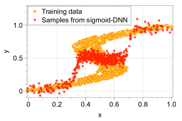
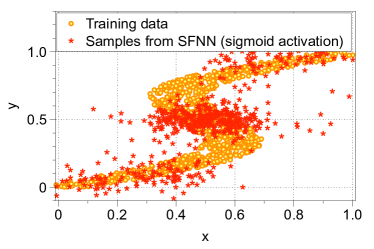
We evaluate the performance of the simple transformations from DNN to SFNN on the MNIST dataset [6] and the synthetic dataset [36], where the former and the latter are popular datasets used for a classification task and a multi-modal (i.e., one-to-many mappings) prediction learning, respectively. In all experiments reported in this paper, we commonly use the softmax and Gaussian with standard deviation of $\sigma_{y}=0.05$ are used for the output probability on classification and regression tasks, respectively. The only first hidden layer of DNN is replaced by a stochastic layer, and we use 500 samples for estimating the expectations in the SFNN inference. As reported in Table 1, we observe that the simple transformation often works well for both tasks: the SFNN and sigmoid-DNN inferences (using same parameters trained by sigmoid-DNN) perform similarly for the classification task and the former significantly outperforms the latter for the multi-modal task (also see Figure 1). It might suggest some possibilities that the expensive SFNN training might not be not necessary, depending on the targeted learning quality. However, in case of ReLU, SFNN performs much worse than ReLU-DNN for the MNIST classification task under the parameter transformation.

Figure 2: (a) Simplified-SFNN (top) and SFNN (bottom). The randomness of the stochastic layer propagates only to its upper layer in the case of Simplified-SFNN. (b) For first 200 epochs, we train a baseline ReLU-DNN. Then, we train simplified-SFNN initialized by the DNN parameters under transformation (8) with $\gamma_{2}=50$. We observe that training ReLU-DNN^∗ directly does not reduce the test error even when network knowledge transferring still holds between the baseline ReLU-DNN and the corresponding ReLU-DNN^∗. (c) As the value of $\gamma_{2}$ increases, knowledge transferring loss measured as $\frac{1}{|D|}\frac{1}{N^{\ell}}\sum\limits_{\mathbf{x}}\sum\limits_{i}\left|h_{i}^{\ell}\left(\mathbf{x}\right)-\widehat{h}_{i}^{\ell}\left(\mathbf{x}\right)\right|$ is decreasing.

Table 2: Classification test error rates [$\%$] on MNIST, where each layer of neural networks contains 800 hidden units. All Simplified-SFNNs are constructed by replacing the first hidden layer of a baseline DNN with stochastic hidden layer. We also consider training DNN and fine-tuning Simplified-SFNN using batch normalization (BN) and dropout (DO). The performance improvements beyond baseline DNN (due to fine-tuning DNN parameters under Simplified-SFNN) are calculated in the bracket.

Inference Model	Training Model	Network Structure	without BN & DO	with BN	with DO
sigmoid-DNN	sigmoid-DNN	2 hidden layers	1.54	1.57	1.25
SFNN	sigmoid-DNN	2 hidden layers	1.56	2.23	1.27
Simplified-SFNN	fine-tuned by Simplified-SFNN	2 hidden layers	1.51	1.5	1.11
sigmoid-DNN∗	fine-tuned by Simplified-SFNN	2 hidden layers	1.48 (0.06)	1.48 (0.09)	1.14 (0.11)
SFNN	fine-tuned by Simplified-SFNN	2 hidden layers	1.51	1.57	1.11
ReLU-DNN	ReLU-DNN	2 hidden layers	1.49	1.25	1.12
SFNN	ReLU-DNN	2 hidden layers	5.73	3.47	1.74
Simplified-SFNN	fine-tuned by Simplified-SFNN	2 hidden layers	1.41	1.17	1.06
ReLU-DNN∗	fine-tuned by Simplified-SFNN	2 hidden layers	1.32 (0.17)	1.16 (0.09)	1.05 (0.07)
SFNN	fine-tuned by Simplified-SFNN	2 hidden layers	2.63	1.34	1.51
ReLU-DNN	ReLU-DNN	3 hidden layers	1.43	1.34	1.24
SFNN	ReLU-DNN	3 hidden layers	17.83	4.15	1.49
Simplified-SFNN	fine-tuned by Simplified-SFNN	3 hidden layers	1.28	1.25	1.04
ReLU-DNN∗	fine-tuned by Simplified-SFNN	3 hidden layers	1.27 (0.16)	1.24 (0.1)	1.03 (0.21)
SFNN	fine-tuned by Simplified-SFNN	3 hidden layers	1.56	1.82	1.16
ReLU-DNN	ReLU-DNN	4 hidden layers	1.49	1.34	1.30
SFNN	ReLU-DNN	4 hidden layers	14.64	3.85	2.17
Simplified-SFNN	fine-tuned by Simplified-SFNN	4 hidden layers	1.32	1.32	1.25
ReLU-DNN∗	fine-tuned by Simplified-SFNN	4 hidden layers	1.29 (0.2)	1.29 (0.05)	1.25 (0.05)
SFNN	fine-tuned by Simplified-SFNN	4 hidden layers	3.44	1.89	1.56

3 Transformation from DNN to SFNN via Simplified-SFNN

In this section, we propose an advanced method to utilize the pre-trained parameters of DNN for training SFNN. As shown in the previous section, simple parameter transformations from DNN to SFNN do not clearly work in general, in particular for activation functions other than sigmoid. Moreover, training DNN does not utilize the stochastic regularizing effect, which is an important benefit of SFNN. To address the issues, we design an intermediate model, called Simplified-SFNN. The proposed model is a special form of stochastic neural network, which approximates certain SFNN by simplifying its upper latent units above stochastic ones. Then, we establish more rigorous connections between three models: DNN $\rightarrow$ Simplified-SFNN $\rightarrow$ SFNN, which leads to an efficient training procedure of the stochastic models utilizing pre-trained parameters of DNN. In our experiments, we evaluate the strategy for various tasks and popular DNN architectures.

3.1 Simplified-SFNN of two hidden layers and non-negative activation functions

For clarity of presentation, we first introduce Simplified-SFNN with two hidden layers and non-negative activation functions, where its extensions to multiple layers and general activation functions are presented in Section 4. We also remark that we primarily describe fully-connected Simplified-SFNNs, but their convolutional versions can also be naturally defined. In Simplified-SFNN of two hidden layers, we assume that the first and second hidden layers consist of stochastic binary hidden units and deterministic ones, respectively. As in (3), the first layer is defined as a binary random vector with $N^{1}$ units, i.e., $\mathbf{h}^{1}\in\{0,1\}^{N^{1}}$, drawn under the following distribution:

$$P\left(\mathbf{h}^{1}\mid\mathbf{x}\right)=\prod\limits_{i=1}^{N^{1}}P\left(h_{i}^{1}\mid\mathbf{x}\right),\text{where}\quad P\left(h_{i}^{1}=1\mid\mathbf{x}\right)=\min\bigg{\{}\alpha_{1}f\left(\mathbf{W}^{1}_{i}\mathbf{x}+b_{i}^{1}\right),1\bigg{\}}.$$ (5)

where $\mathbf{x}$ is the input vector, $\alpha_{1}>0$ is a hyper-parameter for the first layer, and $f:\mathbb{R}\rightarrow\mathbb{R}_{+}$ is some non-negative non-linear activation function with $\left|f^{\prime}(x)\right|\leq 1$ for all $x\in\mathbb{R}$, e.g., ReLU and sigmoid activation functions. Now the second layer is defined as the following deterministic vector with $N^{2}$ units, i.e., $\mathbf{h}^{2}(\mathbf{x})\in\mathbb{R}^{N^{2}}$:

$$\mathbf{h}^{2}\left(\mathbf{x}\right)=\left[f\left(\alpha_{2}\left(\mathbb{E}_{P\left(\mathbf{h}^{1}\mid\mathbf{x}\right)}\left[s\left(\mathbf{W}^{2}_{j}\mathbf{h}^{1}+b_{j}^{2}\right)\right]-s\left(0\right)\right)\right):\forall j\right],$$ (6)

where $\alpha_{2}>0$ is a hyper-parameter for the second layer and $s:\mathbb{R}\rightarrow\mathbb{R}$ is a differentiable function with $|s^{\prime\prime}(x)|\leq 1$ for all $x\in\mathbb{R}$, e.g., sigmoid and tanh functions. In our experiments, we use the sigmoid function for $s(x)$. Here, one can note that the proposed model also has the same computational issues with SFNN in forward and backward passes due to the complex expectation. One can train Simplified-SFNN similarly as SFNN: we use Monte Carlo approximation for estimating the expectation and the (biased) estimator of the gradient for approximating backpropagation inspired by [9] (see Section 3.3 for more details).

We are interested in transferring parameters of DNN to Simplified-SFNN to utilize the training benefits of DNN since the former is much faster to train than the latter. To this end, we consider the following DNN of which $\ell$-th hidden layer is deterministic and defined as follows:

$$\mathbf{\widehat{h}}^{\ell}\left(\mathbf{x}\right)=\left[\leavevmode\nobreak\ \widehat{h}_{i}^{\ell}\left(\mathbf{x}\right)=f\left(\mathbf{\widehat{W}}^{\ell}_{i}\mathbf{\widehat{h}}^{\ell-1}\left(\mathbf{x}\right)+{\widehat{b}}_{i}^{\ell}\right):\forall i\leavevmode\nobreak\ \right],$$ (7)

where $\mathbf{\widehat{h}}^{0}(\mathbf{x})=\mathbf{x}$. As stated in the following theorem, we establish a rigorous way how to initialize parameters of Simplified-SFNN in order to transfer the knowledge stored in DNN.

Theorem 1.

Assume that both DNN and Simplified-SFNN with two hidden layers have same network structure with non-negative activation function $f$. Given parameters $\{\mathbf{\widehat{W}}^{\ell},\mathbf{\widehat{b}}^{\ell}:{\ell=1,2}\}$ of DNN and input dataset $D$, choose those of Simplified-SFNN as follows:

$$\left(\alpha_{1},\mathbf{W}^{1},\leavevmode\nobreak\ \mathbf{b}^{1}\right)\leftarrow\left(\frac{1}{\gamma_{1}},\leavevmode\nobreak\ \mathbf{\widehat{W}}^{1},\leavevmode\nobreak\ \mathbf{\widehat{b}}^{1}\right),\leavevmode\nobreak\ \left(\alpha_{2},\mathbf{W}^{2},\leavevmode\nobreak\ \mathbf{b}^{2}\right)\leftarrow\left(\frac{\gamma_{2}\gamma_{1}}{s^{\prime}\left(0\right)},\leavevmode\nobreak\ \frac{1}{\gamma_{2}}\mathbf{\widehat{W}}^{2},\leavevmode\nobreak\ \frac{1}{\gamma_{1}\gamma_{2}}\mathbf{\widehat{b}}^{2}\right),$$ (8)

where $\gamma_{1}=\underset{i,\mathbf{x}\in D}{{\max}}\leavevmode\nobreak\ \left|f\left(\mathbf{\widehat{W}}^{1}_{i}\mathbf{x}+{\widehat{b}}_{i}^{1}\right)\right|$ and $\gamma_{2}>0$ is any positive constant. Then, for all $j,\mathbf{x}\in D$, it follows that

$$\left|h_{j}^{2}\left(\mathbf{x}\right)-\widehat{h}_{j}^{2}\left(\mathbf{x}\right)\right|\leq\frac{\gamma_{1}\left(\sum_{i}\left|{\widehat{W}}_{ij}^{2}\right|+{\widehat{b}}_{j}^{2}\gamma_{1}^{-1}\right)^{2}}{2s^{\prime}\left(0\right)\gamma_{2}}.\quad$$

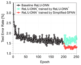
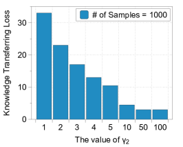
The proof of the above theorem is presented in Section 5.1. Our proof is built upon the first-order Taylor expansion of non-linear function $s(x)$. Theorem 1 implies that one can make Simplified-SFNN represent the function values of DNN with bounded errors using a linear transformation. Furthermore, the errors can be made arbitrarily small by choosing large $\gamma_{2}$, i.e., $\lim\limits_{\gamma_{2}\to\infty}\left|h_{j}^{2}\left(\mathbf{x}\right)-\widehat{h}_{j}^{2}\left(\mathbf{x}\right)\right|=0,$ $\forall j,\mathbf{x}\in D.$ Figure 2 shows that knowledge transferring loss decreases as $\gamma_{2}$ increases on MNIST classification. Based on this, we choose $\gamma_{2}=50$ commonly for all experiments.

3.2 Why Simplified-SFNN ?

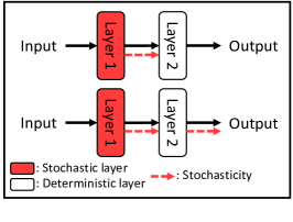
Given a Simplified-SFNN model, the corresponding SFNN can be naturally defined by taking out the expectation in (6). As illustrated in Figure 2, the main difference between SFNN and Simplified-SFNN is that the randomness of the stochastic layer propagates only to its upper layer in the latter, i.e., the randomness of $\mathbf{h}^{1}$ is averaged out at its upper units $\mathbf{h}^{2}$ and does not propagate to $\mathbf{h}^{3}$ or output $y$. Hence, Simplified-SFNN is no longer a Bayesian network. This makes training Simplified-SFNN much easier than SFNN since random samples are not required at some layers and consequently the quality of gradient estimations can also be improved, in particular for unbounded activation functions. Furthermore, one can use the same approximation procedure (2.2) to see that Simplified-SFNN approximates SFNN. However, since Simplified-SFNN still maintains binary random units, it uses approximation steps later, in comparison with DNN. In summary, Simplified-SFNN is an intermediate model between DNN and SFNN, i.e., DNN $\rightarrow$ Simplified-SFNN $\rightarrow$ SFNN.

Table 3: Test negative log-likelihood (NLL) on MNIST and TFD datasets, where each layer of neural networks contains 200 hidden units. All Simplified-SFNNs are constructed by replacing the first hidden layer of a baseline DNN with stochastic hidden layer.

Inference Model	Training Model	MNIST		TFD
		2 Hidden Layers	3 Hidden Layers	2 Hidden Layers	3 Hidden Layers
sigmoid-DNN	sigmoid-DNN	1.409	1.720	-0.064	0.005
SFNN	sigmoid-DNN	0.644	1.076	-0.461	-0.401
Simplified-SFNN	fine-tuned by Simplified-SFNN	1.474	1.757	-0.071	-0.028
SFNN	fine-tuned by Simplified-SFNN	0.619	0.991	-0.509	-0.423
ReLU-DNN	ReLU-DNN	1.747	1.741	1.271	1.232
SFNN	ReLU-DNN	-1.019	-1.021	0.823	1.121
Simplified-SFNN	fine-tuned by Simplified-SFNN	2.122	2.226	0.175	0.343
SFNN	fine-tuned by Simplified-SFNN	-1.290	-1.061	-0.380	-0.193

The above connection naturally suggests the following training procedure for both SFNN and Simplified-SFNN: train a baseline DNN first and then fine-tune its corresponding Simplified-SFNN initialized by the transformed DNN parameters. Finally, the fine-tuned parameters can be used for SFNN as well. We evaluate the strategy for the MNIST classification. The MNIST dataset consists of $28\times 28$ pixel greyscale images, each containing a digit 0 to 9 with 60,000 training and 10,000 test images. For this experiment, we do not use any data augmentation or pre-processing. The loss was minimized using ADAM learning rule [7] with a mini-batch size of 128. We used an exponentially decaying learning rate. Hyper-parameters are tuned on the validation set consisting of the last 10,000 training images. All Simplified-SFNNs are constructed by replacing the first hidden layer of a baseline DNN with stochastic hidden layer. We first train a baseline DNN for first 200 epochs, and the trained parameters of DNN are used for initializing those of Simplified-SFNN. For 50 epochs, we train simplified-SFNN. We choose the hyper-parameter $\gamma_{2}=50$ in the parameter transformation. All Simplified-SFNNs are trained with $M=20$ samples at each epoch, and in the test, we use 500 samples. Table 2 shows that SFNN under the two-stage training always performs better than SFNN under a simple transformation (4) from ReLU-DNN. More interestingly, Simplified-SFNN consistently outperforms its baseline DNN due to the stochastic regularizing effect, even when we train both models using dropout [16] and batch normalization [17]. This implies that the proposed stochastic model can be used for improving the performance of DNNs and it can be also combined with other regularization methods such as dropout batch normalization. In order to confirm the regularization effects, one can again approximate a trained Simplified-SFNN by a new deterministic DNN which we call DNN^∗ and is different from its baseline DNN under the following approximation at upper latent units above binary random units:

$$\mathbb{E}_{P\left(\mathbf{h}^{\ell}\mid\mathbf{x}\right)}\left[s\left(\mathbf{W}^{\ell+1}_{j}\mathbf{h}^{\ell}\right)\right]\backsimeq s\left(\mathbb{E}_{P\left(\mathbf{h}^{\ell}\mid\mathbf{x}\right)}\left[\mathbf{W}^{\ell+1}_{j}\mathbf{h}^{\ell}\right]\right)=s\left(\sum_{i}W^{\ell+1}_{ij}P\left(h^{\ell}_{i}=1\mid\mathbf{x}\right)\right).$$ (9)

We found that DNN^∗ using fined-tuned parameters of Simplified-SFNN also outperforms the baseline DNN as shown in Table 2 and Figure 2.

3.3 Training Simplified-SFNN

The parameters of Simplified-SFNN can be learned using a variant of the backpropagation algorithm [29] in a similar manner to DNN. However, in contrast to DNN, there are two computational issues for simplified-SFNN: computing expectations with respect to stochastic units in forward pass and computing gradients in back pass. One can notice that both are intractable since they require summations over all possible configurations of all stochastic units. First, in order to handle the issue in forward pass, we use the following Monte Carlo approximation for estimating the expectation:

$$\mathbb{E}_{P\left(\mathbf{h}^{1}\mid\mathbf{x}\right)}\left[s\left(\mathbf{W}^{2}_{j}\mathbf{h}^{1}+b_{j}^{2}\right)\right]\backsimeq\frac{1}{M}\sum\limits_{m=1}^{M}s\left(\mathbf{W}^{2}_{j}\mathbf{h}^{(m)}+b_{j}^{2}\right),$$

where $\mathbf{h}^{(m)}\sim P\left(\mathbf{h}^{1}\mid\mathbf{x}\right)$ and $M$ is the number of samples. This random estimator is unbiased and has relatively low variance [8] since its accuracy does not depend on the dimensionality of $\mathbf{h}^{1}$ and one can draw samples from the exact distribution. Next, in order to handle the issue in back pass, we use the following approximation inspired by [9]:

$$\frac{\partial}{\partial\mathbf{W}^{2}_{j}}\mathbb{E}_{P\left(\mathbf{h}^{1}\mid\mathbf{x}\right)}\left[s\left(\mathbf{W}^{2}_{j}\mathbf{h}^{1}+b_{j}^{2}\right)\right] \backsimeq\frac{1}{M}\sum\limits_{m}\frac{\partial}{\partial\mathbf{W}^{2}_{j}}s\left(\mathbf{W}^{2}_{j}\mathbf{h}^{(m)}+b_{j}^{2}\right),$$

$$\frac{\partial}{\partial\mathbf{W}^{1}_{i}}\mathbb{E}_{P\left(\mathbf{h}^{1}\mid\mathbf{x}\right)}\left[s\left(\mathbf{W}^{2}_{j}\mathbf{h}^{1}+b_{j}^{2}\right)\right] \backsimeq\frac{W^{2}_{ij}}{M}\sum\limits_{m}s^{\prime}\left(\mathbf{W}^{2}_{j}\mathbf{h}^{(m)}+b_{j}^{2}\right)\frac{\partial}{\partial\mathbf{W}^{1}_{i}}P\left(h_{i}^{1}=1\mid\mathbf{x}\right),$$

where $\mathbf{h}^{(m)}\sim P\left(\mathbf{h}^{1}\mid\mathbf{x}\right)$ and $M$ is the number of samples. In our experiments, we commonly choose $M=20$.

4 Extensions of Simplified-SFNN

In this section, we describe how the network knowledge transferring between Simplified-SFNN and DNN, i.e., Theorem 1, generalizes to multiple layers and general activation functions.

4.1 Extension to multiple layers

A deeper Simplified-SFNN with $L$ hidden layers can be defined similarly as the case of $L=2$. We also establish network knowledge transferring between Simplified-SFNN and DNN with $L$ hidden layers as stated in the following theorem. Here, we assume that stochastic layers are not consecutive for simpler presentation, but the theorem is generalizable for consecutive stochastic layers.

Theorem 2.

Assume that both DNN and Simplified-SFNN with $L$ hidden layers have same network structure with non-negative activation function $f$. Given parameters $\{\mathbf{\widehat{W}}^{\ell},\mathbf{\widehat{b}}^{\ell}:{\ell=1,\dots,L}\}$ of DNN and input dataset $D$, choose the same ones for Simplified-SFNN initially and modify them for each $\ell$-th stochastic layer and its upper layer as follows:

$$\alpha_{\ell}\leftarrow\frac{1}{\gamma_{\ell}},\left(\alpha_{\ell+1},\mathbf{W}^{\ell+1},\leavevmode\nobreak\ \mathbf{b}^{\ell+1}\right)\leftarrow\left(\frac{\gamma_{\ell}\gamma_{\ell+1}}{s^{\prime}\left(0\right)},\leavevmode\nobreak\ \frac{\mathbf{\widehat{W}}^{\ell+1}}{\gamma_{\ell+1}},\leavevmode\nobreak\ \frac{\mathbf{\widehat{b}}^{\ell+1}}{\gamma_{\ell}\gamma_{\ell+1}}\right),$$ (10)

where $\gamma_{\ell}=\max\limits_{i,\mathbf{x}\in D}\leavevmode\nobreak\ \left|f\left(\mathbf{\widehat{W}}^{\ell}_{i}\mathbf{h}^{\ell-1}(\mathbf{x})+{\widehat{b}}_{i}^{\ell}\right)\right|$ and $\gamma_{\ell+1}$ is any positive constant. Then, it follows that

$$\lim\limits_{\begin{subarray}{c}\gamma_{\ell+1}\to\infty\\ \forall\leavevmode\nobreak\ \text{stochastic hidden layer}\leavevmode\nobreak\ \ell\end{subarray}}\left|h_{j}^{L}\left(\mathbf{x}\right)-\widehat{h}_{j}^{L}\left(\mathbf{x}\right)\right|=0,\quad\forall j,\mathbf{x}\in D.$$

The above theorem again implies that it is possible to transfer knowledge from DNN to Simplified-SFNN by choosing large $\gamma_{l+1}$. The proof of Theorem 2 is similar to that of Theorem 1 and given in Section 5.2.

4.2 Extension to general activation functions

In this section, we describe an extended version of Simplified-SFNN which can utilize any activation function. To this end, we modify the definitions of stochastic layers and their upper layers by introducing certain additional terms. If the $\ell$-th hidden layer is stochastic, then we slightly modify the original definition (5) as follows:

$$P\left(\mathbf{h}^{\ell}\mid\mathbf{x}\right)=\prod\limits_{i=1}^{N^{\ell}}P\left(h_{i}^{\ell}\mid\mathbf{x}\right)\text{with}\leavevmode\nobreak\ \leavevmode\nobreak\ P\left(h_{i}^{\ell}=1\mid\mathbf{x}\right)=\min\bigg{\{}\alpha_{\ell}f\left(\mathbf{W}^{1}_{i}\mathbf{x}+b_{i}^{1}+\frac{1}{2}\right),1\bigg{\}},$$

where $f:\mathbb{R}\rightarrow\mathbb{R}$ is a non-linear (possibly, negative) activation function with $\left|f^{\prime}(x)\right|\leq 1$ for all $x\in\mathbb{R}$. In addition, we re-define its upper layer as follows:

$$\mathbf{h}^{\ell+1}\left(\mathbf{x}\right)=\bigg{[}f\Big{(}\alpha_{\ell+1}\Big{(}\mathbb{E}_{P\left(\mathbf{h}^{\ell}\mid\mathbf{x}\right)}\left[s\left(\mathbf{W}^{\ell+1}_{j}\mathbf{h}^{\ell}+b_{j}^{\ell+1}\right)\right]-s\left(0\right){-\frac{s^{\prime}\left(0\right)}{2}\sum_{i}W_{ij}^{\ell+1}}\Big{)}\Big{)}:\forall j\bigg{]},$$

where $\mathbf{h}^{0}(\mathbf{x})=\mathbf{x}$ and $s:\mathbb{R}\rightarrow\mathbb{R}$ is a differentiable function with $\left|s^{\prime\prime}(x)\right|\leq 1$ for all $x\in\mathbb{R}$.

Under this general Simplified-SFNN model, we also show that transferring network knowledge from DNN to Simplified-SFNN is possible as stated in the following theorem. Here, we again assume that stochastic layers are not consecutive for simpler presentation.

Theorem 3.

Assume that both DNN and Simplified-SFNN with $L$ hidden layers have same network structure with non-linear activation function $f$. Given parameters $\{\mathbf{\widehat{W}}^{\ell},\mathbf{\widehat{b}}^{\ell}:{\ell=1,\dots,L}\}$ of DNN and input dataset $D$, choose the same ones for Simplified-SFNN initially and modify them for each $\ell$-th stochastic layer and its upper layer as follows:

$$\alpha_{\ell}\leftarrow\frac{1}{2\gamma_{\ell}},\left(\alpha_{\ell+1},\mathbf{W}^{\ell+1},\leavevmode\nobreak\ \mathbf{b}^{\ell+1}\right)\leftarrow\left(\frac{2\gamma_{\ell}\gamma_{\ell+1}}{s^{\prime}(0)},\leavevmode\nobreak\ \frac{\mathbf{\widehat{W}}^{\ell+1}}{\gamma_{\ell+1}},\leavevmode\nobreak\ \frac{\mathbf{\widehat{b}}^{\ell+1}}{2\gamma_{\ell}\gamma_{\ell+1}}\right),$$

where $\gamma_{\ell}=\underset{i,\mathbf{x}\in D}{{\max}}\leavevmode\nobreak\ \left|f\left(\mathbf{\widehat{W}}^{\ell}_{i}\mathbf{h}^{\ell-1}(\mathbf{x})+{\widehat{b}}_{i}^{\ell}\right)\right|$, and $\gamma_{\ell+1}$ is any positive constant. Then, it follows that

$$\lim\limits_{\begin{subarray}{c}\gamma_{\ell+1}\to\infty\\ \forall\leavevmode\nobreak\ \text{stochastic hidden layer}\leavevmode\nobreak\ \ell\end{subarray}}\left|h_{j}^{L}\left(\mathbf{x}\right)-\widehat{h}_{j}^{L}\left(\mathbf{x}\right)\right|=0,\quad\forall j,\mathbf{x}\in D.$$

We omit the proof of the above theorem since it is somewhat direct adaptation of that of Theorem 2.

5 Proofs of Theorems

5.1 Proof of Theorem 1

First consider the first hidden layer, i.e., stochastic layer. Let $\gamma_{1}=\max\limits_{i,\mathbf{x}\in D}f\left(\mathbf{\widehat{W}}^{1}_{i}\mathbf{x}+{\widehat{b}}_{i}^{1}\right)$ be the maximum value of hidden units in DNN. If we initialize the parameters $\left(\alpha_{1},\mathbf{W}^{1},\leavevmode\nobreak\ \mathbf{b}^{1}\right)\leftarrow\left(\frac{1}{\gamma_{1}},\leavevmode\nobreak\ \mathbf{\widehat{W}}^{1},\leavevmode\nobreak\ \mathbf{\widehat{b}}^{1}\right)$, then the marginal distribution of each hidden unit $i$ becomes

$$P\left(h_{i}^{1}=1\mid\mathbf{x},\mathbf{W}^{1},\mathbf{b}^{1}\right)=min\bigg{\{}\alpha_{1}f\left(\mathbf{\widehat{W}}^{1}_{i}\mathbf{x}+{\widehat{b}}_{i}^{1}\right),1\bigg{\}}=\frac{1}{\gamma_{1}}f\left(\mathbf{\widehat{W}}^{1}_{i}\mathbf{x}+{\widehat{b}}_{i}^{1}\right),\leavevmode\nobreak\ \forall i,\mathbf{x}\in D.$$ (11)

Next consider the second hidden layer. From Taylor’s theorem, there exists a value $z$ between $0$ and $x$ such that $s(x)=s(0)+s^{\prime}(0)x+R(x)$, where $R(x)=\frac{s^{\prime\prime}(z)x^{2}}{2!}$. Since we consider a binary random vector, i.e., $\mathbf{h}^{1}\in\{0,1\}^{N^{1}}$, one can write

$$\mathbb{E}_{P\left(\mathbf{h}^{1}\mid\mathbf{x}\right)}\left[s\left(\beta_{j}\left(\mathbf{h}^{1}\right)\right)\right]$$

$$=\sum\limits_{\mathbf{h}^{1}}\left(s\left(0\right)+s^{\prime}\left(0\right)\beta_{j}\left(\mathbf{h}^{1}\right)+R\left(\beta_{j}\left(\mathbf{h}^{1}\right)\right)\right)P\left(\mathbf{h}^{1}\mid\mathbf{x}\right)$$

$$=s\left(0\right)+s^{\prime}\left(0\right)\left(\sum\limits_{i}W^{2}_{ij}P(h_{i}^{1}=1\mid\mathbf{x})+b_{j}^{2}\right)+\mathbb{E}_{P\left(\mathbf{h}^{1}\mid\mathbf{x}\right)}\left[R(\beta_{j}(\mathbf{h}^{1}))\right],$$ (12)

where $\beta_{j}\left(\mathbf{h}^{1}\right):=\mathbf{W}^{2}_{j}\mathbf{h}^{1}+b_{j}^{2}$ is the incoming signal. From (6) and (11), for every hidden unit $j$, it follows that

$$h_{j}^{2}\left(\mathbf{x};\mathbf{W}^{2},\mathbf{b}^{2}\right)= f\Bigg{(}\alpha_{2}\Bigg{(}s^{\prime}(0)\left(\frac{1}{\gamma_{1}}\sum\limits_{i}W^{2}_{ij}{\widehat{h}}_{i}^{1}\left(\mathbf{x}\right)+b_{j}^{2}\right)+\mathbb{E}_{P\left(\mathbf{h}^{1}\mid\mathbf{x}\right)}\left[R\left(\beta_{j}\left(\mathbf{h}^{1}\right)\right)\right]\Bigg{)}\Bigg{)}.$$

Since we assume that $\left|f^{\prime}(x)\right|\leq 1$, the following inequality holds:

$$\left\lvert h_{j}^{2}(\mathbf{x};\mathbf{W}^{2},\mathbf{b}^{2})-f\left(\alpha_{2}s^{\prime}(0)\left(\frac{1}{\gamma_{1}}\sum\limits_{i}W^{2}_{ij}{\widehat{h}}_{i}^{1}(\mathbf{x})+b_{j}^{2}\right)\right)\right\rvert$$

$$\leq\left|\alpha_{2}\mathbb{E}_{P\left(\mathbf{h}^{1}\mid\mathbf{x}\right)}\left[R(\beta_{j}(\mathbf{h}^{1}))\right]\right|\leq\frac{\alpha_{2}}{2}\mathbb{E}_{P(\mathbf{h}^{1}\mid\mathbf{x})}\left[\left(\mathbf{W}^{2}_{j}\mathbf{h}^{1}+b_{j}^{2}\right)^{2}\right],$$ (13)

where we use $|s^{\prime\prime}(z)|<1$ for the last inequality. Therefore, it follows that

$$\left|h_{j}^{2}\left(\mathbf{x};\mathbf{W}^{2},\mathbf{b}^{2}\right)-\widehat{h}_{j}^{2}\left(\mathbf{x};\mathbf{\widehat{W}}^{2},\mathbf{\widehat{b}}^{2}\right)\right|\leq\frac{\gamma_{1}\left(\sum_{i}\left|{\widehat{W}}_{ij}^{2}\right|+{\widehat{b}}_{j}^{2}\gamma_{1}^{-1}\right)^{2}}{2s^{\prime}(0)\gamma_{2}},\quad\forall j,$$

since we set $\left(\alpha_{2},\mathbf{W}^{2},\leavevmode\nobreak\ \mathbf{b}^{2}\right)\leftarrow\left(\frac{\gamma_{2}\gamma_{1}}{s^{\prime}(0)},\leavevmode\nobreak\ \frac{\mathbf{\widehat{W}}^{2}}{\gamma_{2}},\leavevmode\nobreak\ \frac{\gamma_{1}^{-1}}{\gamma_{2}}\mathbf{\widehat{b}}^{2}\right)$. This completes the proof of Theorem 1.

5.2 Proof of Theorem 2

For the proof of Theorem 2, we first state the two key lemmas on error propagation in Simplified-SFNN.

Lemma 4.

Assume that there exists some positive constant $B$ such that

$$\left|h_{i}^{\ell-1}\left(\mathbf{x}\right)-\widehat{h}_{i}^{\ell-1}\left(\mathbf{x}\right)\right|\leq B,\quad\forall i,\mathbf{x}\in D,$$

and the $\ell$-th hidden layer of Simplified-SFNN is standard deterministic layer as defined in (7). Given parameters $\{\mathbf{\widehat{W}}^{\ell},\mathbf{\widehat{b}}^{\ell}\}$ of DNN, choose same ones for Simplified-SFNN. Then, the following inequality holds:

$$\left|h_{j}^{\ell}\left(\mathbf{x}\right)-\widehat{h}_{j}^{\ell}\left(\mathbf{x}\right)\right|\leq BN^{\ell-1}{\widehat{W}}_{\max}^{\ell},\quad\forall j,\mathbf{x}\in D.$$

where ${\widehat{W}}_{\max}^{\ell}=\max\limits_{ij}\left|{\widehat{W}}_{ij}^{\ell}\right|$.

Proof..

See Section 5.3. $\Box$

Lemma 5.

Assume that there exists some positive constant $B$ such that

$$\left|h_{i}^{\ell-1}\left(\mathbf{x}\right)-\widehat{h}_{i}^{\ell-1}\left(\mathbf{x}\right)\right|\leq B,\quad\forall i,\mathbf{x}\in D,$$

and the $\ell$-th hidden layer of simplified-SFNN is stochastic layer. Given parameters $\{\mathbf{\widehat{W}}^{\ell},\mathbf{\widehat{W}}^{\ell+1},\mathbf{\widehat{b}}^{\ell},\mathbf{\widehat{b}}^{\ell+1}\}$ of DNN, choose those of Simplified-SFNN as follows:

$$\alpha_{\ell}\leftarrow\frac{1}{\gamma_{\ell}},\left(\alpha_{\ell+1},\mathbf{W}^{\ell+1},\leavevmode\nobreak\ \mathbf{b}^{\ell+1}\right)\leftarrow\left(\frac{\gamma_{\ell}\gamma_{\ell+1}}{s^{\prime}\left(0\right)},\leavevmode\nobreak\ \frac{\mathbf{\widehat{W}}^{\ell+1}}{\gamma_{\ell+1}},\leavevmode\nobreak\ \frac{\mathbf{\widehat{b}}^{\ell+1}}{\gamma_{\ell}\gamma_{\ell+1}}\right),$$

where $\gamma_{\ell}=\max\limits_{j,\mathbf{x}\in D}\leavevmode\nobreak\ \left|f\left(\mathbf{\widehat{W}}^{\ell}_{j}\mathbf{h}^{\ell-1}(\mathbf{x})+{\widehat{b}}_{j}^{\ell}\right)\right|$ and $\gamma_{\ell+1}$ is any positive constant. Then, for all $j,\mathbf{x}\in D$, it follows that

$$\left|h_{k}^{\ell+1}\left(\mathbf{x}\right)-\widehat{h}_{k}^{\ell+1}\left(\mathbf{x}\right)\right|\leq BN^{\ell-1}N^{\ell}{\widehat{W}}_{\max}^{\ell}{\widehat{W}}_{\max}^{\ell+1}+\left|\frac{\gamma_{\ell}\left(N^{\ell}{\widehat{W}}_{\max}^{\ell+1}+{\widehat{b}}_{\max}^{\ell+1}\gamma_{\ell}^{-1}\right)^{2}}{2s^{\prime}(0)\gamma_{\ell+1}}\right|,$$

where ${\widehat{b}}_{\max}^{\ell}=\max\limits_{j}\left|{\widehat{b}}_{j}^{\ell}\right|$ and ${\widehat{W}}_{\max}^{\ell}=\max\limits_{ij}\left|{\widehat{W}}_{ij}^{\ell}\right|$.

Proof..

See Section 5.4. $\Box$

Assume that $\ell$-th layer is first stochastic hidden layer in Simplified-SFNN. Then, from Theorem 1, we have

$$\left|h_{j}^{\ell+1}\left(\mathbf{x}\right)-\widehat{h}_{j}^{\ell+1}\left(\mathbf{x}\right)\right|\leq\left|\frac{\gamma_{\ell}\left(N^{\ell}{\widehat{W}}_{\max}^{\ell+1}+{\widehat{b}}_{\max}^{\ell+1}\gamma_{\ell}^{-1}\right)^{2}}{2s^{\prime}(0)\gamma_{\ell+1}}\right|,\quad\forall j,\mathbf{x}\in D.$$ (14)

According to Lemma 4 and 5, the final error generated by the right hand side of (14) is bounded by

$$\frac{\tau_{\ell}\gamma_{\ell}\left(N^{\ell}{\widehat{W}}_{\max}^{\ell+1}+{\widehat{b}}_{\max}^{\ell+1}\gamma_{\ell}^{-1}\right)^{2}}{2s^{\prime}\left(0\right)\gamma_{\ell+1}},$$ (15)

where $\tau_{\ell}=\prod\limits_{\ell^{\prime}=l+2}^{L}\left(N^{\ell^{\prime}-1}{\widehat{W}}_{\max}^{\ell^{\prime}}\right).$ One can note that every error generated by each stochastic layer is bounded by (15). Therefore, for all $j,\mathbf{x}\in D$, it follows that

$$\left|h_{j}^{L}\left(\mathbf{x}\right)-\widehat{h}_{j}^{L}\left(\mathbf{x}\right)\right|\leq\sum\limits_{\ell:\text{stochastic hidden layer}}\left(\frac{\tau_{\ell}\gamma_{\ell}\left(N^{\ell}{\widehat{W}}_{\max}^{\ell+1}+{\widehat{b}}_{\max}^{\ell+1}\gamma_{\ell}^{-1}\right)^{2}}{2s^{\prime}\left(0\right)\gamma_{\ell+1}}\right).$$

From above inequality, we can conclude that

$$\lim\limits_{\begin{subarray}{c}\gamma_{\ell+1}\to\infty\\ \forall\leavevmode\nobreak\ \text{stochastic hidden layer}\leavevmode\nobreak\ \ell\end{subarray}}\left|h_{j}^{L}\left(\mathbf{x}\right)-\widehat{h}_{j}^{L}\left(\mathbf{x}\right)\right|=0,\quad\forall j,\mathbf{x}\in D.$$

This completes the proof of Theorem 2.

5.3 Proof of Lemma 4

From assumption, there exists some constant $\epsilon_{i}$ such that $\left|\epsilon_{i}\right|<B$ and

$$h_{i}^{\ell-1}\left(\mathbf{x}\right)=\widehat{h}_{i}^{\ell-1}\left(\mathbf{x}\right)+\epsilon_{i},\leavevmode\nobreak\ \leavevmode\nobreak\ \forall i,\mathbf{x}.$$

By definition of standard deterministic layer, it follows that

$$h_{j}^{\ell}\left(\mathbf{x}\right)=f\left(\sum\limits_{i}{\widehat{W}}^{\ell}_{ij}{h}_{i}^{\ell-1}\left(\mathbf{x}\right)+{\widehat{b}}_{j}^{\ell-1}\right)=f\left(\sum\limits_{i}{\widehat{W}}^{\ell}_{ij}{\widehat{h}}_{i}^{\ell-1}\left(\mathbf{x}\right)+\sum\limits_{i}{\widehat{W}}^{\ell}_{ij}\epsilon_{i}+{\widehat{b}}_{j}^{\ell}\right).$$

Since we assume that $\left|f^{\prime}(x)\right|\leq 1$, one can conclude that

$$\left|h_{j}^{\ell}\left(\mathbf{x}\right)-f\left(\sum\limits_{i}{\widehat{W}}^{\ell}_{ij}{\widehat{h}}_{i}^{\ell-1}\left(\mathbf{x}\right)+{\widehat{b}}_{j}^{\ell}\right)\right|\leq\left|\sum\limits_{i}{\widehat{W}}^{\ell}_{ij}\epsilon_{i}\right|\leq B\left|\sum\limits_{i}{\widehat{W}}^{\ell}_{ij}\right|\leq BN^{\ell-1}{\widehat{W}}_{\max}^{\ell}.$$

This completes the proof of Lemma 4.

5.4 Proof of Lemma 5

From assumption, there exists some constant $\epsilon^{\ell-1}_{i}$ such that $\left|\epsilon^{\ell-1}_{i}\right|<B$ and

$$h_{i}^{\ell-1}\left(\mathbf{x}\right)=\widehat{h}_{i}^{\ell-1}\left(\mathbf{x}\right)+\epsilon^{\ell-1}_{i},\leavevmode\nobreak\ \leavevmode\nobreak\ \forall i,\mathbf{x}.$$ (16)

Let $\gamma_{\ell}=\max\limits_{j,\mathbf{x}\in D}\leavevmode\nobreak\ \left|f\left(\mathbf{\widehat{W}}^{\ell}_{j}\mathbf{h}^{\ell-1}(\mathbf{x})+{\widehat{b}}_{j}^{\ell}\right)\right|$ be the maximum value of hidden units. If we initialize the parameters $\left(\alpha_{\ell},\mathbf{W}^{\ell},\leavevmode\nobreak\ \mathbf{b}^{\ell}\right)\leftarrow\left(\frac{1}{\gamma_{\ell}},\leavevmode\nobreak\ \mathbf{\widehat{W}}^{\ell},\leavevmode\nobreak\ \mathbf{\widehat{b}}^{\ell}\right)$, then the marginal distribution becomes

$$P\left(h_{j}^{\ell}=1\mid\mathbf{x},\mathbf{W}^{\ell},\mathbf{b}^{\ell}\right) =\min\bigg{\{}\alpha_{\ell}f\left(\mathbf{\widehat{W}}^{\ell}_{j}\mathbf{h}^{\ell-1}\left(\mathbf{x}\right)+{\widehat{b}}_{j}^{\ell}\right),1\bigg{\}}$$

$$=\frac{1}{\gamma_{\ell}}f\left(\mathbf{\widehat{W}}^{\ell}_{j}\mathbf{h}^{\ell-1}\left(\mathbf{x}\right)+{\widehat{b}}_{j}^{\ell}\right),\leavevmode\nobreak\ \forall j,\mathbf{x}.$$

From (16), it follows that

$$P\left(h_{j}^{\ell}=1\mid\mathbf{x},\mathbf{W}^{\ell},\mathbf{b}^{\ell}\right)=\frac{1}{\gamma_{\ell}}f\left(\mathbf{\widehat{W}}^{\ell}_{j}\mathbf{\widehat{h}}^{\ell-1}\left(\mathbf{x}\right)+\sum\limits_{i}{\widehat{W}}^{\ell}_{ij}\epsilon^{\ell-1}_{i}+{\widehat{b}}_{j}^{\ell}\right),\quad\forall j,\mathbf{x}.$$

Similar to Lemma 4, there exists some constant $\epsilon^{\ell}_{j}$ such that $\left|\epsilon^{\ell}_{j}\right|<BN^{\ell-1}{\widehat{W}}_{\max}^{\ell}$ and

$$P\left(h_{j}^{\ell}=1\mid\mathbf{x},\mathbf{W}^{\ell},\mathbf{b}^{\ell}\right)=\frac{1}{\gamma_{\ell}}\left(\widehat{h}_{j}^{\ell}\left(\mathbf{x}\right)+\epsilon^{\ell}_{j}\right),\leavevmode\nobreak\ \leavevmode\nobreak\ \forall j,\mathbf{x}.$$ (17)

Next, consider the upper hidden layer of stochastic layer. From Taylor’s theorem, there exists a value $z$ between $0$ and $t$ such that $s(x)=s(0)+s^{\prime}(0)x+R(x)$, where $R(x)=\frac{s^{\prime\prime}(z)x^{2}}{2!}$. Since we consider a binary random vector, i.e., $\mathbf{h}^{\ell}\in\{0,1\}^{N^{\ell}}$, one can write

$$\mathbb{E}_{P(\mathbf{h}^{\ell}\mid\mathbf{x})}[s(\beta_{k}(\mathbf{h}^{\ell}))] =\sum\limits_{\mathbf{h}^{\ell}}\left(s(0)+s^{\prime}(0)\beta_{k}(\mathbf{h}^{\ell})+R\left(\beta_{k}(\mathbf{h}^{\ell})\right)\right)P(\mathbf{h}^{\ell}\mid\mathbf{x})$$

$$=s(0)+s^{\prime}(0)\left(\sum\limits_{j}W^{\ell+1}_{jk}P(h_{j}^{\ell}=1\mid\mathbf{x})+b_{k}^{\ell+1}\right)+\sum\limits_{\mathbf{h}^{\ell}}R(\beta_{k}(\mathbf{h}^{\ell}))P(\mathbf{h}^{\ell}\mid\mathbf{x}),$$

where $\beta_{k}(\mathbf{h}^{\ell})=\mathbf{W}^{\ell+1}_{k}\mathbf{h}^{\ell}+b_{k}^{\ell+1}$ is the incoming signal. From (17) and above equation, for every hidden unit $k$, we have

$$h_{k}^{\ell+1}(\mathbf{x};\mathbf{W}^{\ell+1},\mathbf{b}^{\ell+1})$$

$$=f\Bigg{(}\alpha_{\ell+1}\Bigg{(}s^{\prime}(0)\Bigg{(}\frac{1}{\gamma_{\ell}}\left(\sum\limits_{j}W^{\ell+1}_{jk}{\widehat{h}}_{j}^{\ell}(\mathbf{x})+\sum\limits_{j}W^{\ell+1}_{jk}\epsilon^{\ell}_{j}\right)+b_{k}^{\ell+1}\Bigg{)}+\mathbb{E}_{P(\mathbf{h}^{\ell}\mid\mathbf{x})}\left[R(\beta_{k}(\mathbf{h}^{\ell}))\right]\Bigg{)}\Bigg{)}.$$

Since we assume that $|f^{\prime}(x)|<1$, the following inequality holds:

$$\Bigg{|}h_{k}^{\ell+1}(\mathbf{x};\mathbf{W}^{\ell+1},\mathbf{b}^{\ell+1})-f\left(\alpha_{\ell+1}s^{\prime}(0)\left(\frac{1}{\gamma_{\ell}}\sum\limits_{j}W^{\ell+1}_{ij}{\widehat{h}}_{j}^{\ell}(\mathbf{x})+b_{j}^{\ell+1}\right)\right)\Bigg{|}$$

$$\leq\left|\frac{\alpha_{\ell+1}s^{\prime}(0)}{\gamma_{\ell}}\sum\limits_{j}W^{\ell+1}_{jk}\epsilon^{\ell}_{j}+\alpha_{\ell+1}\mathbb{E}_{P(\mathbf{h}^{\ell}\mid\mathbf{x})}\left[R(\beta_{k}(\mathbf{h}^{\ell}))\right]\right|$$

$$\leq\left|\frac{\alpha_{\ell+1}s^{\prime}(0)}{\gamma_{\ell}}\sum\limits_{j}W^{\ell+1}_{jk}\epsilon^{\ell}_{j}\right|+\left|\frac{\alpha_{\ell+1}}{2}\mathbb{E}_{P(\mathbf{h}^{\ell}\mid\mathbf{x})}\left[\left(\mathbf{W}^{\ell+1}_{k}\mathbf{h}^{\ell}+b_{k}^{\ell+1}\right)^{2}\right]\right|,$$ (18)

where we use $|s^{\prime\prime}(z)|<1$ for the last inequality. Therefore, it follows that

$$\left|h_{k}^{\ell+1}\left(\mathbf{x}\right)-\widehat{h}_{k}^{\ell+1}\left(\mathbf{x}\right)\right|\leq \leavevmode\nobreak\ BN^{\ell-1}N^{\ell}{\widehat{W}}_{\max}^{\ell}{\widehat{W}}_{\max}^{\ell+1}+\left|\frac{\gamma_{\ell}\left(N^{\ell}{\widehat{W}}_{\max}^{\ell+1}+{\widehat{b}}_{\max}^{\ell+1}\gamma_{\ell}^{-1}\right)^{2}}{2s^{\prime}(0)\gamma_{\ell+1}}\right|,$$

since we set $\left(\alpha_{\ell+1},\mathbf{W}^{\ell+1},\leavevmode\nobreak\ \mathbf{b}^{\ell+1}\right)\leftarrow\left(\frac{\gamma_{\ell+1}\gamma_{\ell}}{s^{\prime}(0)},\leavevmode\nobreak\ \frac{\mathbf{\widehat{W}}^{\ell+1}}{\gamma_{\ell+1}},\leavevmode\nobreak\ \frac{\gamma_{\ell}^{-1}\mathbf{\widehat{b}}^{\ell+1}}{\gamma_{\ell+1}}\right)$. This completes the proof of Lemma 5.

6 Experimental Results

Figure 3: The overall structures of (a) Lenet-5, (b) NIN, (c) WRN with 16 layers, and (d) WRN with 28 layers. The red feature maps correspond to the stochastic ones. In case of WRN, we introduce one ($v^{\prime}=3$) and two ($v^{\prime}=2$) stochastic feature maps.

We present several experimental results for both multi-modal and classification tasks on MNIST [6], Toronto Face Database (TFD) [37], CASIA [3], CIFAR-10, CIFAR-100 [14] and SVHN [26]. The softmax and Gaussian with the standard deviation of 0.05 are used as the output probability for the classification task and the multi-modal prediction, respectively. In all experiments, we first train a baseline model, and the trained parameters are used for further fine-tuning those of Simplified-SFNN.

6.1 Multi-modal regression

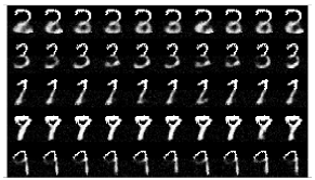
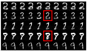
We first verify that it is possible to learn one-to-many mapping via Simplified-SFNN on the TFD, MNIST and CASIA datasets. The TFD dataset consists of $48\times 48$ pixel greyscale images, each containing a face image of 900 individuals with 7 different expressions. Similar to [9], we use 124 individuals with at least 10 facial expressions as data. We randomly choose 100 individuals with 1403 images for training and the remaining 24 individuals with 326 images for the test. We take the mean of face images per individual as the input and set the output as the different expressions of the same individual. The MNIST dataset consists of greyscale images, each containing a digit 0 to 9 with 60,000 training and 10,000 test images. For this experiments, each pixel of every digit images is binarized using its grey-scale value similar to [9]. We take the upper half of the MNIST digit as the input and set the output as the lower half of it. We remark that both tasks are commonly performed in recent other works to test the multi-modal learning using SFNN [9, 34]. The CASIA dataset consists of greyscale images, each containing a handwritten Chinese character. We use 10 offline isolated characters produced by 345 writers as data. We randomly choose 300 writers with 3000 images for training and the remaining 45 writers with 450 images for testing. We take the radical character per writer as the input and set the output as either the related character or the radical character itself of the same writer (see Figure 6). The bicubic interpolation [4] is used for re-sizing all images as $32\times 32$ pixels.

Figure 4: Generated samples for predicting the lower half of the MNIST digit given the upper half. (a) The original digits and the corresponding inputs. The generated samples from (b) sigmoid-DNN, (c) SFNN under the simple transformation, and (d) SFNN fine-tuned by Simplified-SFNN. We remark that SFNN fine-tuned by Simplified-SFNN can generate more various samples (e.g., red rectangles) from same inputs better than SFNN under the simple transformation.

For both TFD and MNIST datasets, we use fully-connected DNNs as the baseline models similar to other works [9, 34]. All Simplified-SFNNs are constructed by replacing the first hidden layer of a baseline DNN with stochastic hidden layer. The loss was minimized using ADAM learning rule [7] with a mini-batch size of 128. We used an exponentially decaying learning rate. We train Simplified-SFNNs with $M=20$ samples at each epoch, and in the test, we use 500 samples. We use 200 hidden units for each layer of neural networks in two experiments. Learning rate is chosen from {0.005 , 0.002, 0.001, … , 0.0001}, and the best result is reported for both tasks. Table 3 reports the test negative log-likelihood on TFD and MNIST. One can note that SFNNs fine-tuned by Simplified-SFNN consistently outperform SFNN under the simple transformation.

For the CASIA dataset, we choose fully-convolutional network (FCN) models [2] as the baseline ones, which consists of convolutional layers followed by a fully-convolutional layer. In a similar manner to the case of fully-connected networks, one can define a stochastic convolution layer, which considers the input feature map as a binary random matrix and generates the output feature map as defined in (6). For this experiment, we use a baseline model, which consists of convolutional layers followed by a fully convolutional layer. The convolutional layers have 64, 128 and 256 filters respectively. Each convolutional layer has a4×4receptive field applied with a stride of 2 pixel. All Simplified-SFNNs are constructed by replacing the first hidden feature maps of baseline models with stochastic ones. The loss was minimized using ADAM learning rule [7] with a mini-batch size of 128. We used an exponentially decaying learning rate. We train Simplified-SFNNs with $M=20$ samples at each epoch, and in the test, we use 100 samples due to the memory limitations. One can note that SFNNs fine-tuned by Simplified-SFNN outperform SFNN under the simple transformation as reported in Table 4 and Figure 6.

Table 4: Test NLL on CASIA dataset. All Simplified-SFNNs are constructed by replacing the first hidden feature maps of baseline models with stochastic ones.

Inference Model	Training Model	2 Conv Layers	3 Conv Layers
FCN	FCN	3.89	3.47
SFNN	FCN	2.61	1.97
Simplified-SFNN	fine-tuned by Simplified-SFNN	3.83	3.47
SFNN	fine-tuned by Simplified-SFNN	2.45	1.81

Figure 5: (a) The input-output Chinese characters. The generated samples from (b) FCN, (c) SFNN under the simple transformation and (d) SFNN fine-tuned by Simplified-SFNN. Our model can generate the multi-modal outputs (red rectangle), while SFNN under the simple transformation cannot.

Figure 6: Test error rates of WRN^∗ per each training epoch on CIFAR-100. One can note that the performance gain is more significant when we introduce more stochastic layers.

6.2 Classification

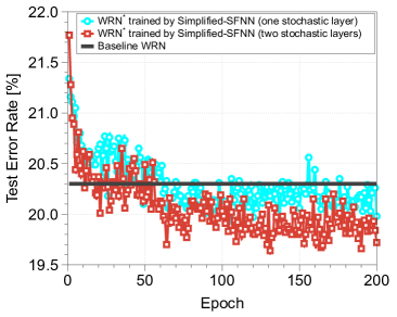
We also evaluate the regularization effect of Simplified-SFNN for the classification tasks on CIFAR-10, CIFAR-100 and SVHN. The CIFAR-10 and CIFAR-100 datasets consist of 50,000 training and 10,000 test images. They have 10 and 100 image classes, respectively. The SVHN dataset consists of 73,257 training and 26,032 test images. It consists of a house number 0 to 9 collected by Google Street View. Similar to [39], we pre-process the data using global contrast normalization and ZCA whitening. For these datasets, we design a convolutional version of Simplified-SFNN using convolutional neural networks such as Lenet-5 [6], NIN [13] and WRN [39]. All Simplified-SFNNs are constructed by replacing a hidden feature map of a baseline models, i.e., Lenet-5, NIN and WRN, with stochastic one as shown in Figure 3. We use WRN with 16 and 28 layers for SVHN and CIFAR datasets, respectively, since they showed state-of-the-art performance as reported by [39]. In case of WRN, we introduce up to two stochastic convolution layers. Similar to [39], the loss was minimized using the stochastic gradient descent method with Nesterov momentum. The minibatch size is set to 128, and weight decay is set to 0.0005. For 100 epochs, we first train baseline models, i.e., Lenet-5, NIN and WRN, and trained parameters are used for initializing those of Simplified-SFNNs. All Simplified-SFNNs are trained with $M=5$ samples and the test error is only measured by the approximation (9). The test errors of baseline models are measured after training them for 200 epochs similar to [39]. All models are trained using dropout [16] and batch normalization [17]. Table 5 reports the classification error rates on CIFAR-10, CIFAR-100 and SVHN. Due to the regularization effects, Simplified-SFNNs consistently outperform their baseline DNNs. In particular, WRN^∗ of 28 layers and 36 million parameters outperforms WRN by 0.08$\%$ on CIFAR-10 and 0.58$\%$ on CIFAR-100. Figure 6 shows that the error rate is decreased more when we introduce more stochastic layers, but it increases the fine-tuning time-complexity of Simplified-SFNN.

Table 5: Test error rates [$\%$] on CIFAR-10, CIFAR-100 and SVHN. The error rates for WRN are from our experiments, where original ones reported in [39] are in the brackets. Results with $\dagger$ are obtained using the horizontal flipping and random cropping augmentation.

Inference model	Training Model	CIFAR-10	CIFAR-100	SVHN
Lenet-5	Lenet-5	37.67	77.26	11.18
Lenet-5∗	fine-tuned by Simplified-SFNN	33.58	73.02	9.88
NIN	NIN	9.51	32.66	3.21
NIN∗	fine-tuned by Simplified-SFNN	9.33	30.81	3.01
WRN	WRN	4.22 (4.39)$\dagger$	20.30 (20.04)$\dagger$	3.25$\dagger$
WRN∗	fine-tuned by Simplified-SFNN (one stochastic layer)	4.21$\dagger$	19.98$\dagger$	3.09$\dagger$
WRN∗	fine-tuned by Simplified-SFNN (two stochastic layers)	4.14$\dagger$	19.72$\dagger$	3.06$\dagger$

7 Conclusion

In order to develop an efficient training method for large-scale SFNN, this paper proposes a new intermediate stochastic model, called Simplified-SFNN. We establish the connection between three models, i.e., DNN $\rightarrow$ Simplified-SFNN $\rightarrow$ SFNN, which naturally leads to an efficient training procedure of the stochastic models utilizing pre-trained parameters of DNN. This connection naturally leads an efficient training procedure of the stochastic models utilizing pre-trained parameters and architectures of DNN. Using several popular DNNs including Lenet-5, NIN, FCN and WRN, we show how they can be effectively transferred to the corresponding stochastic models for both multi-modal and non-multi-modal tasks. We believe that our work brings a new angle for training stochastic neural networks, which would be of broader interest in many related applications.

References

- [1] Ruiz, F.R., AUEB, M.T.R. and Blei, D. The generalized reparameterization gradient. In Advances in Neural Information Processing Systems (NIPS), 2016.
- [2] Long, J., Shelhamer, E. and Darrell, T. Fully convolutional networks for semantic segmentation. In Proceedings of the IEEE Conference on Computer Vision and Pattern Recognition (CVPR), 2015.
- [3] Liu, C.L., Yin, F., Wang, D.H. and Wang, Q.F. CASIA online and offline Chinese handwriting databases. In International Conference on Document Analysis and Recognition (ICDAR), 2011.
- [4] Keys, R. Cubic convolution interpolation for digital image processing. In IEEE transactions on acoustics, speech, and signal processing, 1981.
- [5] Neal, R.M. Learning stochastic feedforward networks. Department of Computer Science, University of Toronto, 1990.
- [6] LeCun, Y., Bottou, L., Bengio, Y. and Haffner, P. Gradient-based learning applied to document recognition. Proceedings of the IEEE, 1998.
- [7] Kingma, D. and Ba, J. Adam: A method for stochastic optimization. arXiv preprint arXiv:1412.6980, 2014.
- [8] Tang, Y. and Salakhutdinov, R.R. Learning stochastic feedforward neural networks. In Advances in Neural Information Processing Systems (NIPS), 2013.
- [9] Raiko, T., Berglund, M., Alain, G. and Dinh, L. Techniques for learning binary stochastic feedforward neural networks. arXiv preprint arXiv:1406.2989, 2014.
- [10] Wan, L., Zeiler, M., Zhang, S., Cun, Y.L. and Fergus, R. Regularization of neural networks using dropconnect. In International Conference on Machine Learning (ICML), 2013.
- [11] Krizhevsky, A., Sutskever, I. and Hinton, G.E. Imagenet classification with deep convolutional neural networks. In Advances in Neural Information Processing Systems (NIPS), 2012.
- [12] Goodfellow, I.J., Warde-Farley, D., Mirza, M., Courville, A. and Bengio, Y. Maxout networks. In International Conference on Machine Learning (ICML), 2013.
- [13] Lin, M., Chen, Q. and Yan, S. Network in network. In International Conference on Learning Representations (ICLR), 2014.
- [14] Krizhevsky, A. and Hinton, G. Learning multiple layers of features from tiny images. Master’s thesis, Department of Computer Science, University of Toronto, 2009.
- [15] Blundell, C., Cornebise, J., Kavukcuoglu, K. and Wierstra, D. Weight uncertainty in neural networks. In International Conference on Machine Learning (ICML), 2015.
- [16] Hinton, G.E., Srivastava, N., Krizhevsky, A., Sutskever, I. and Salakhutdinov, R.R. Improving neural networks by preventing co-adaptation of feature detectors. arXiv preprint arXiv:1207.0580, 2012.
- [17] Ioffe, S. and Szegedy, C. Batch normalization: Accelerating deep network training by reducing internal covariate shift. In International Conference on Machine Learning (ICML), 2015.
- [18] Salakhutdinov, R. and Hinton, G.E. Deep boltzmann machines. In Conference on Artificial Intelligence and Statistics (AISTATS), 2009.
- [19] Neal, R.M. Connectionist learning of belief networks. Artificial intelligence, 1992.
- [20] Hinton, G.E., Osindero, S. and Teh, Y.W. A fast learning algorithm for deep belief nets. Neural computation, 2006.
- [21] Poon, H. and Domingos, P. Sum-product networks: A new deep architecture. In Conference on Uncertainty in Artificial Intelligence (UAI), 2011.
- [22] Chen, T., Goodfellow, I. and Shlens, J. Net2Net: Accelerating Learning via Knowledge Transfer. arXiv preprint arXiv:1511.05641, 2015.
- [23] Maass, W. Networks of spiking neurons: the third generation of neural network models. Neural Networks, 1997.
- [24] Hinton, G., Deng, L., Yu, D., Dahl, G.E., Mohamed, A.R., Jaitly, N., Senior, A., Vanhoucke, V., Nguyen, P., Sainath, T.N. and Kingsbury, B. Deep neural networks for acoustic modeling in speech recognition: The shared views of four research groups. IEEE Signal Processing Magazine, 2012.
- [25] Zeiler, M.D. and Fergus, R. Stochastic pooling for regularization of deep convolutional neural networks. In International Conference on Learning Representations (ICLR), 2013.
- [26] Netzer, Y., Wang, T., Coates, A., Bissacco, A., Wu, B. and Ng, A.Y. Reading digits in natural images with unsupervised feature learning. In NIPS Workshop on Deep Learning and Unsupervised Feature Learning, 2011.
- [27] Courbariaux, M., Bengio, Y. and David, J.P. BinaryConnect: Training Deep Neural Networks with binary weights during propagations. arXiv preprint arXiv:1511.00363, 2015.
- [28] Gulcehre, C., Moczulski, M., Denil, M. and Bengio, Y. Noisy activation functions. arXiv preprint arXiv:1603.00391, 2016.
- [29] Rumelhart, D.E., Hinton, G.E. and Williams, R.J. Learning internal representations by error propagation. In Neurocomputing: Foundations of research, MIT Press, 1988.
- [30] Robbins, H. and Monro, S. A stochastic approximation method. Annals of Mathematical Statistics, 1951.
- [31] Ba, J. and Frey, B. Adaptive dropout for training deep neural networks. In Advances in Neural Information Processing Systems (NIPS), 2013.
- [32] Kingma, D.P. and Welling, M. Auto-encoding variational bayes. arXiv preprint arXiv:1312.6114, 2013.
- [33] Nair, V. and Hinton, G.E. Rectified linear units improve restricted boltzmann machines. In International Conference on Machine Learning (ICML), 2010.
- [34] Gu, S., Levine, S., Sutskever, I. and Mnih, A. MuProp: Unbiased backpropagation for stochastic neural networks. arXiv preprint arXiv:1511.05176, 2015.
- [35] Bengio, Y., Léonard, N. and Courville, A. Estimating or propagating gradients through stochastic neurons for conditional computation. arXiv preprint arXiv:1308.3432, 2013.
- [36] Bishop, C.M. Mixture density networks. Aston University, 1994.
- [37] Susskind, J.M., Anderson, A.K. and Hinton, G.E. The toronto face database. Department of Computer Science, University of Toronto, Toronto, ON, Canada, Tech. Rep, 3, 2010.
- [38] Saul, L.K., Jaakkola, T. and Jordan, M.I. Mean field theory for sigmoid belief networks. Artificial intelligence, 1996.
- [39] Zagoruyko, S. and Komodakis, N. Wide residual networks. arXiv preprint arXiv:1605.07146, 2016.
- [40] Huang, G., Sun, Y., Liu, Z., Sedra, D. and Weinberger, K.Q. Deep networks with stochastic depth. In European Conference on Computer Vision (ECCV), 2016.
- [41] Goodfellow, I., Pouget-Abadie, J., Mirza, M., Xu, B., Warde-Farley, D., Ozair, S., Courville, A. and Bengio, Y. Generative adversarial nets. In Advances in Neural Information Processing Systems (NIPS), 2014.
- [42] Zaremba, W. and Sutskever, I. Reinforcement learning neural Turing machines. arXiv preprint arXiv:1505.00521, 362, 2015.
- [43] Szegedy, C., Liu, W., Jia, Y., Sermanet, P., Reed, S., Anguelov, D., Erhan, D., Vanhoucke, V. and Rabinovich, A. Going deeper with convolutions. In Proceedings of the IEEE Conference on Computer Vision and Pattern Recognition (CVPR), 2015.
- [44] Simonyan, K. and Zisserman, A. Very deep convolutional networks for large-scale image recognition. arXiv preprint arXiv:1409.1556, 2014.
- [45] He, K., Zhang, X., Ren, S. and Sun, J. Identity mappings in deep residual networks. In European Conference on Computer Vision (ECCV), 2016.
- [46] Salimans, T. and Kingma, D.P. Weight normalization: A simple reparameterization to accelerate training of deep neural networks. In Advances in Neural Information Processing Systems (NIPS), 2016.
- [47] http://www.cs.nyu.edu/˜roweis/data.html