Minkowski Operations of Sets
with Application to Robot Localization

Abstract

This papers shows that using separators, which is a pair of two complementary contractors, we can easily and efficiently solve the localization problem of a robot with sonar measurements in an unstructured environment. We introduce separators associated with the Minkowski sum and the Minkowski difference in order to facilitate the resolution. A test-case is given in order to illustrate the principle of the approach.

1 Introduction

Interval analysis [15] is a tool which makes it possible to compute with sets even when nonlinear functions are involved [11] in the definition of the sets. Interval methods are generally used to solve equations or optimization problems [6] but can also been used to solve set-membership problems where the sets are represented by subpavings [8]. The efficiency of interval algorithms can be improved by the use of contractors [3] or (separators [7] which correspond to pairs of contractors).

This paper deals with localization of a robot with sonar rangefinders in a unstructured environment. This problem is considered as difficult due to the fact that the sonar returns a measurement under the form of an impact point inside an emission cone. This specific type of measurement makes the problem partially observable. Moreover, our environment is not represented by geometric features such as segments or disks, but by an image which cannot be translated into equations. Now, as shown by Sliwka [18], an unstructured map can be cast into a contractor form which allows us to use contractor/separator algebra.

Here, we propose first to use a separator-based method to perform a reliable simulation necessary to generate realistic data (see, e.g., [19] for a survey on reliable simulation). Then, once these data have been generated, we consider the inverse problem, i.e., the robot localization with large-cone sonar measurements in an unstructured map. This problem has never been considered yet, to our knowledge at least in an unstructured environment (see e.g., [10, 12, 9, 13, 4] in the case where the map is made with geometrical features). We will also show the link with Minkowski operations and propose separator counterparts for these operations.

Section 2 recalls the basic notions on contractors and separators needed to understand our approach. Section 3 presents the concept of set-to-set transform and shows how our localization problem can be solved with separators. Section 4 proposes to formulate the Minkowski operations as a specific set-to-set transform, corresponding to translations. Section 5 illustrates the application of the Minkowski operation to the problem of localization of a robot in an unstructured environment. Section 6 concludes the paper.

2 Contractors and Separators

This section recalls the basic notions on intervals, contractors and separators that are needed to understand the contribution of this paper. An interval of $\mathbb{R}$ is a closed connected set of $\mathbb{R}$. A box $\left[\mathbf{x}\right]$ of $\mathbb{R}^{n}$ is the Cartesian product of $n$ intervals.

A contractor $\mathcal{C}$ is an operator $\mathbb{IR}^{n}\mapsto\mathbb{IR}^{n}$ such that

$$\begin{array}[]{lll}\mathcal{C}([\mathbf{x}])\subset[\mathbf{x}]&&\text{(contractance)}\\ {}[\mathbf{x}]\subset\left[\mathbf{y}\right]\text{ }\Rightarrow\text{ }\mathcal{C}([\mathbf{x}])\subset\mathcal{C}([\mathbf{y}]).&&\text{(monotonicity)}\end{array}$$ (1)

We define the inclusion between two contractors $\mathcal{C}_{1}$ and $\mathcal{C}_{2}$ as follows:

$$\mathcal{C}_{1}\subset\mathcal{C}_{2}\Leftrightarrow\forall\left[\mathbf{x}\right]\in\mathbb{IR}^{n}\text{, }\mathcal{C}_{1}([\mathbf{x}])\subset\mathcal{C}_{2}([\mathbf{x}]).$$ (2)

A set $\mathbb{X}$ is consistent (See Figure 1) with the contractor $\mathcal{C}$ (we will write $\mathbb{X}\sim\mathcal{C}$) if for all $\left[\mathbf{x}\right]$, we have

$$\mathcal{C}([\mathbf{x}])\cap\mathbb{X}=[\mathbf{x}]\cap\mathbb{X}.$$ (3)

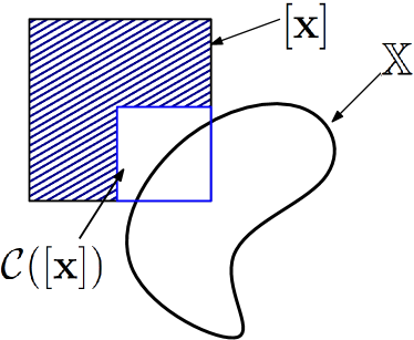
Figure 1: Contractor consistent with to the set $\mathbb{X}$

Two contractors $\mathcal{C}$ and $\mathcal{C}_{1}$ are equivalent (we will write $\mathcal{C}\sim\mathcal{C}_{1}$) if we have:

$$\mathbb{X}\sim\mathcal{C}\Leftrightarrow\mathbb{X}\sim\mathcal{C}_{1}.$$ (4)

A contractor $\mathcal{C}$ is minimal if for any other contractor $\mathcal{C}_{1}$, we have the following implication

$$\mathcal{C}\sim\mathcal{C}_{1}\Rightarrow\mathcal{C}\subset\mathcal{C}_{1}.$$ (5)

Example 1. The minimal contractor $\mathcal{C}_{\mathbb{X}}$ consistent with the set

$$\mathbb{X}=\left\{\mathbf{x}\in\mathbb{R}^{2},(x_{1}-2)^{2}+(x_{2}-2.5)^{2}\in\left[1,4\right]\right\}$$ (6)

can be built using a forward-backward constraint propagation [2] [5]. The contractor $\mathcal{C}_{\mathbb{X}}$ can be used by a paver to obtain an outer approximation for $\mathbb{X}$. This is illustrated by Figure 2 (left) where $\mathcal{C}_{\mathbb{X}}$ removes parts of the space outside $\mathbb{X}$ (painted light-gray). But due to the consistency property (see Equation (3)) $\mathcal{C}_{\mathbb{X}}$ has no effect on boxes included in $\mathbb{X}$. A box partially included in $\mathbb{X}$ can not be eliminated and is bisected, except if its length is larger than an given value $\varepsilon$. The contractor $\mathcal{C}_{\mathbb{X}}$ only provides an outer approximation of $\mathbb{X}$.

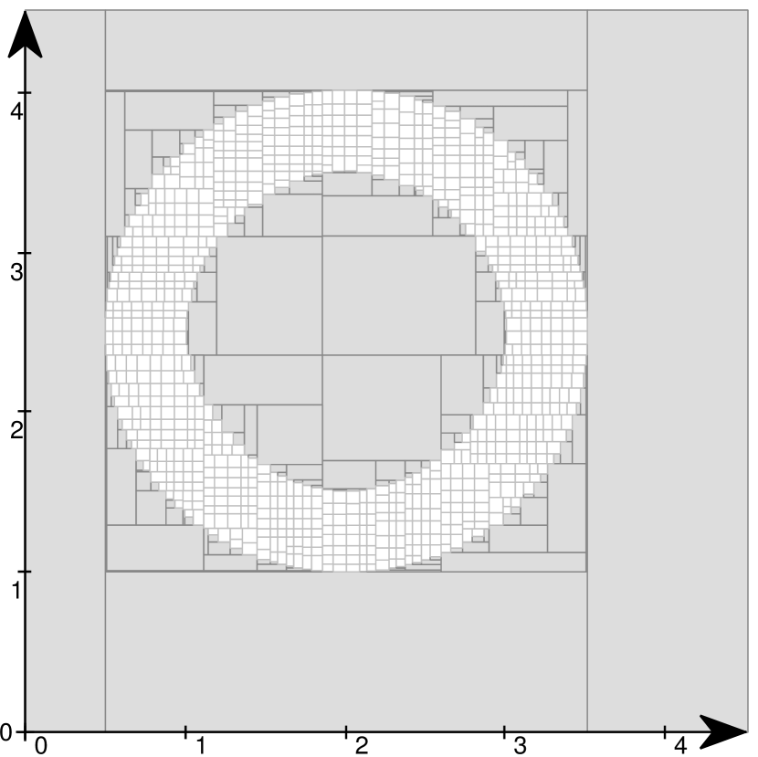
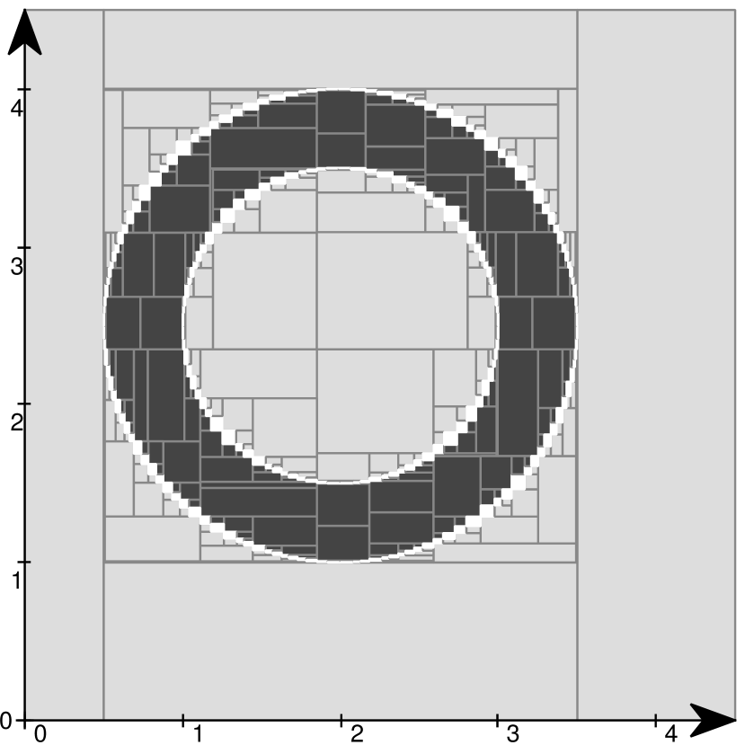
Figure 2: Paving associated to Example 1, Left: paving obtained using the contractor, Right: paving obtained using the separator. Dark gray boxes belong $\mathbb{X}$ (the ring); light gray boxes are outside $\mathbb{X}$. No conclusion can be given on the white boxes.

If $\mathcal{C}_{1}$ and $\mathcal{C}_{2}$ are two contractors, we define the following operations [3].

$$(\mathcal{C}_{1}\cap\mathcal{C}_{2})([\mathbf{x}]) = \mathcal{C}_{1}([\mathbf{x}])\cap\mathcal{C}_{2}([\mathbf{x}])$$ (7)

$$(\mathcal{C}_{1}\sqcup\mathcal{C}_{2})([\mathbf{x}]) = \mathcal{C}_{1}([\mathbf{x}])\sqcup\mathcal{C}_{2}([\mathbf{x}])$$ (8)

$$(\mathcal{C}_{1}\circ\mathcal{C}_{2})([\mathbf{x}]) = \mathcal{C}_{1}\left(\mathcal{C}_{2}([\mathbf{x}])\right)$$ (9)

where $\sqcup$ is the union hull defined by

$$[\mathbf{x}]\sqcup[\mathbf{y}]=\left[[\mathbf{x}]\cup[\mathbf{y}]\right].$$ (10)

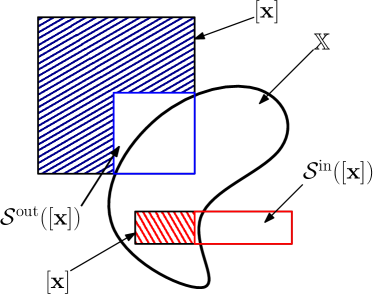
Figure 3: Illustration of a separator on two different initial boxes. The outer contractor removes the blue dashed area and the red dashed area is removed by the inner contractor

In order to characterize an inner and outer approximation of the solution set, we introduce the notion of separator.
A separator $\mathcal{S}$ is a pair of contractors $\left\{\mathcal{S}^{\text{in}},\mathcal{S}^{\text{out}}\right\}$ such that, for all $\left[\mathbf{x}\right]\in\mathbb{IR}^{n}$, we have

$$\begin{array}[]{lll}\mathcal{S}^{\text{in}}(\left[\mathbf{x}\right])\cup\mathcal{S}^{\text{out}}([\mathbf{x}])=\left[\mathbf{x}\right]&&\text{(complementarity).}\end{array}\text{ }$$ (11)

A set $\mathbb{X}$ is consistent with the separator $\mathcal{S}$ (we will write $\mathbb{X}\sim\mathcal{S}$), if

$$\mathbb{X}\sim\mathcal{S}^{\text{out}}\text{ and }\overline{\mathbb{X}}\sim\mathcal{S}^{\text{in}}\text{,}$$ (12)

where $\overline{\mathbb{X}}=\{\mathbf{x}\ |\ \mathbf{x}\notin\mathbb{X}\}$. This notion of separator is illustrated by Figure 3.
We define the inclusion between two separators $\mathcal{S}_{1}$ and $\mathcal{S}_{2}$ as follows

$$\mathcal{S}_{1}\subset\mathcal{S}_{2}\Leftrightarrow\mathcal{S}_{1}^{\text{in}}\subset\mathcal{S}_{2}^{\text{in}}\text{ and }\mathcal{S}_{1}^{\text{out}}\subset\mathcal{S}_{2}^{\text{out}}.$$ (13)

A separator $\mathcal{S}$ is minimal if

$$\mathcal{S}_{1}\subset\mathcal{S}\Rightarrow\mathcal{S}_{1}=\mathcal{S}.$$ (14)

It is trivial to check that $\mathcal{S}$ is minimal implies that the two contractors $\mathcal{S}^{\text{in}}$ and $\mathcal{S}^{\text{out}}$ are both minimal. If we define the following operations

$$\begin{array}[]{cccc}\mathcal{S}_{1}\cap\mathcal{S}_{2}&=&\left\{\mathcal{S}_{1}^{\text{in}}\cup\mathcal{S}_{2}^{\text{in}},\mathcal{S}_{1}^{\text{out}}\cap\mathcal{S}_{2}^{\text{out}}\right\}&\text{(intersection)}\\ \mathcal{S}_{1}\cup\mathcal{S}_{2}&=&\left\{\mathcal{S}_{1}^{\text{in}}\cap\mathcal{S}_{2}^{\text{in}},\mathcal{S}_{1}^{\text{out}}\cup\mathcal{S}_{2}^{\text{out}}\right\}&\text{(union)}\end{array}$$ (15)

then we have [7]

$$\left\{\begin{array}[]{ccc}\mathcal{S}_{1}&\sim&\mathbb{X}_{1}\\ \mathcal{S}_{2}&\sim&\mathbb{X}_{2}\end{array}\right.\Rightarrow\left\{\begin{array}[]{ccc}\mathcal{S}_{1}\cap\mathcal{S}_{2}&\sim&\mathbb{X}_{1}\cap\mathbb{X}_{2}\\ \mathcal{S}_{1}\cup\mathcal{S}_{2}&\sim&\mathbb{X}_{1}\cup\mathbb{X}_{2}\end{array}\right.$$ (16)

Other operations on separators such as the complement or the projection can also be considered [7].

Example 2. Consider the set $\mathbb{X}$ of Example 1. From the contractor consistent with

$$\mathbb{\overline{X}}=\left\{\mathbf{x}\in\mathbb{R}^{2},(x_{1}-2)^{2}+(x_{2}-2.5)^{2}\notin\left[1,4\right]\right\},$$ (17)

we can build a separator $\mathcal{S}_{\mathbb{X}}$ for $\mathbb{X}$. An inner and outer approximation of $\mathbb{X}$ obtained by a paver based on $\mathcal{S}_{\mathbb{X}}$ is depicted on Figure 2. The dark gray area is inside $\mathbb{X}$ and light gray is outside. The minimality property of the separators can be observed by the fact that all contracted boxes of the subpaving touch the boundary of $\mathbb{X}$. Therefore, we are now able to quantify the pessimism introduced by the paver.

3 Set-to-set Transform

Notation. Consider a function

$$\mathbf{f}:\left\{\begin{array}[]{ccc}\mathbb{R}^{n}\times\mathbb{R}^{p}&\longrightarrow&\mathbb{R}^{m}\\ (\mathbf{a},\mathbf{p})&\longrightarrow&\mathbf{f}(\mathbf{a},\mathbf{p})\end{array}\right.$$ (18)

For a given $\mathbf{p}\in\mathbb{R}^{p}$, $\mathbb{A}\subset\mathbb{R}^{n}$, $\mathbb{B}\subset\mathbb{R}^{m}$, $\mathbb{Z}\subset\mathbb{R}^{n}\times\mathbb{R}^{p}$ , we shall use the following notations:

$$\begin{array}[]{cl}\mathbf{f}(\mathbb{A},\mathbf{p})&=\left\{\mathbf{b}|\exists\mathbf{a}\in\mathbb{A},\,\mathbf{b}=\mathbf{f}(\mathbf{a},\mathbf{p})\right\}\\ \mathbf{f}^{-1}(\mathbb{B})&=\left\{\mathbf{z}=(\mathbf{a},\mathbf{p})\,|\exists\mathbf{b}\in\mathbb{B},\,\mathbf{b}=\mathbf{f}(\mathbf{a},\mathbf{p})\right\}\\ proj_{\mathbf{p}}(\mathbb{Z})&=\left\{\mathbf{p}\,|\exists\mathbf{a},\,(\mathbf{a},\mathbf{p})\in\mathbb{Z}\right\}\\ \overline{\mathbb{Z}}&=\left\{\mathbf{z}\,|\,\mathbf{z}\notin\mathbb{Z}\right\}\end{array}$$ (19)

Many sets that are defined with quantifiers can be defined in terms of projection, inversion, complement and composition.

An important problem where these operations occur is the set-to-set transform which is now defined.

Set-to-set transform. Consider the set defined by :

$$\mathbb{P}=\{\mathbf{p}\in\mathbb{R}^{p}\mid\mathbf{f}(\mathbb{A},\mathbf{p})\subset\mathbb{B}\}.$$ (20)

The vector $\mathbf{p}$ corresponds to a parameter vector associated to a transformation. A transformation $\mathbf{p}$ is consistent, if after transformation of $\mathbb{A}$, the set $\mathbb{A}$ is included inside $\mathbb{B}$. We have

$$\begin{array}[]{cl}&\mathbf{f}(\mathbb{A},\mathbf{p})\subset\mathbb{B}\\ \Leftrightarrow&\forall\mathbf{a}\in\mathbb{A},\mathbf{f}(\mathbf{a},\mathbf{p})\in\mathbb{B}\\ \Leftrightarrow&\neg\exists\mathbf{a}\in\mathbb{A},\mathbf{f}(\mathbf{a},\mathbf{p})\in\overline{\mathbb{B}}\\ \Leftrightarrow&\neg\exists\mathbf{a}\in\mathbb{A},(\mathbf{a},\mathbf{p})\in\mathbf{f}^{-1}\left(\overline{\mathbb{B}}\right)\\ \Leftrightarrow&\neg\exists\mathbf{a},(\mathbf{a},\mathbf{p})\in\mathbb{A}\times\mathbb{R}^{p}\,\wedge\,(\mathbf{a},\mathbf{p})\in\mathbf{f}^{-1}\left(\overline{\mathbb{B}}\right).\end{array}$$ (21)

As a consequence

$$\mathbb{P}=\overline{proj_{\mathbf{p}}\{\left(\mathbb{A}\times\mathbb{R}^{p}\right)\cap\mathbf{f}^{-1}\left(\overline{\mathbb{B}}\right)\}}.$$ (22)

Therefore, if we have separators $\mathcal{S}_{\mathbb{A}},\mathcal{S}_{\mathbb{B}}$ for $\mathbb{A},\mathbb{B}$ then a separator $\mathcal{S}_{\mathbb{P}}$ for $\mathbb{P}$ can be obtained using the separator algebra [7]. It is given by

$$\mathcal{S}_{\mathbb{P}}=\overline{proj_{\mathbf{p}}\{\left(\mathbb{\mathcal{S}_{\mathbb{A}}}\times\mathcal{S}_{\mathbb{R}^{p}}\right)\cap\mathbf{f}^{-1}\left(\overline{\mathcal{S}_{\mathbb{B}}}\right)\}}.$$ (23)

Combining this separator with a paver, we are able to obtain an inner and outer approximation of $\mathbb{P}$.

Example 1: A robot at position (0,0) in inside an environment defined by the map

$$\mathbb{M}=\{\mathbf{x}\in\mathbb{R}^{2}\mid x_{1}<5\text{ or }x_{2}<3\}.$$ (24)

It emits an ultrasonic sound in the cone with angles $\frac{\pi}{4}\pm\frac{\pi}{24}$. For a simulation purpose, we want to compute the distance returned by the sonar. This distance corresponds to the shortest distance inside the emission cone to the complementary of the map:

$$d=\inf\{d\mid\mathbf{f}(\mathbb{S}_{1},d)\cap\overline{\mathbb{M}}\neq\emptyset\}$$

or equivalently

$$d=\sup\{d\mid\mathbf{f}(\mathbb{S}_{1},d)\subset\mathbb{M}\},$$ (25)

where $\mathbb{S}_{1}$ is the unit cone defined by

$$\mathbb{S}_{1}=\{(x,y)\mid x^{2}+y^{2}<1\text{ and }atan2(y,x)\in[\frac{5\pi}{24},\frac{7\pi}{24}]\}.$$ (26)

and $\mathbf{f}(\mathbf{x},d)=d\cdot\mathbf{x}$ is the scaling function. To solve our problem, we first characterize the set:

$$\mathbb{D}=\{d\mid\mathbf{f}(\mathbb{S}_{1},d)\subset\mathbb{M}\}$$ (27)

which corresponds to a set-to-set transform problem and we get

$$[0,6.2988]\subset\mathbb{D}\subset[0,6.3085].$$ (28)

The situation is depicted on Figure 4. As a consequence, the true distance $d$ returned by the sensor satisfies $d\in[6.2988,6.3085]$

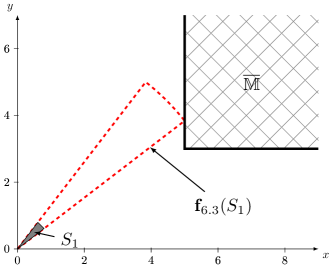
Figure 4: The map $\mathbb{M}$ is represented by the white space outside the hatched area while the unit pie $\mathbb{S}_{1}$ is painted in gray. The red pie represents the lower upper bound of $\mathbb{D}$ which almost touches the border of the map.

4 Minkowski sum and difference

Minkowski operations are used in morphological mathematics to perform dilation or inflation of sets. As it will be shown in Section 4, it can also be used for localization. Efficient algorithms (see e.g., [17]) have been proposed to perform Minkowski operations with sets represented by subpavings. In this section, we show Minkowski sum and difference can be see as a set-to-set transform. This will allow us to build separators for these Minkowski operations.

4.1 Minkowski difference

Given two sets $\mathbb{A}\subset\mathcal{P}(\mathbb{R}^{n})$, $\mathbb{B}\subset\mathcal{P}(\mathbb{R}^{n})$, the Minkowski difference [16], denoted $\ominus$, defined by

$$\mathbb{B}\ominus\mathbb{A} =\{\mathbf{p}\mid\mathbb{A}+\mathbf{p}\subset\mathbb{B}\}.$$ (29)

Proposition 1. Given two separator $\mathcal{S}_{\mathbb{A}}$ and $\mathcal{S}_{\mathbb{B}}$ for $\mathbb{A}$ and $\mathbb{B}$. Define the Minkowski difference of two separators as

$$\mathcal{S}_{\mathbb{B}}\ominus\mathcal{S}_{\mathbb{A}}=\overline{proj_{\mathbf{p}}\{\left(\mathbb{\mathcal{S}_{\mathbb{A}}}\times\mathcal{S}_{\mathbb{R}^{n}}\right)\cap\mathbf{f}^{-1}\left(\overline{\mathcal{S}_{\mathbb{B}}}\right)\}}$$ (30)

where $\mathbf{f}(\mathbf{p},\mathbf{a})=\mathbf{a}+\mathbf{p}$. The operator $\mathcal{S}_{\mathbb{B}}\ominus\mathcal{S}_{\mathbb{A}}$is a separator for $\mathbb{B}\ominus\mathbb{A}$.

Proof. Computing the Minkowski difference can be seen as a specific set-to-set transform problem where $\mathbf{f}(\mathbf{p},\mathbf{a})=\mathbf{a}+\mathbf{p}$ , i.e., the transformation corresponds to a translation of vector $\mathbf{p}$. As a consequence

$$\mathbb{B}\ominus\mathbb{A}=\overline{proj_{\mathbf{p}}\{\left(\mathbb{A}\times\mathbb{R}^{p}\right)\cap\mathbf{f}^{-1}\left(\overline{\mathbb{B}}\right)\}}.\blacksquare$$ (31)

A separator can thus be built for $\mathbb{B}\ominus\mathbb{A}$ and a paver is then able to characterize $\mathbb{B}\ominus\mathbb{A}.$

Example 2: Let $\mathbb{A}$ be a rectangle of side’s length of 4 x 2, and $\mathbb{B}$ be a disk of radius 5. The resulting solution set $\mathbb{B}\ominus\mathbb{A}$ is depicted in Figure 5.

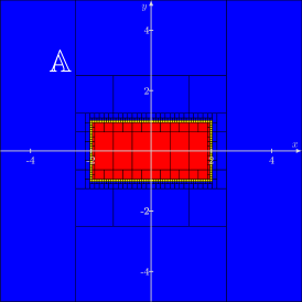
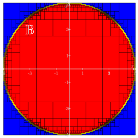
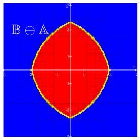
Figure 5: Minkowski difference of the disk $\mathbb{B}$ and the rectangle $\mathbb{A}$

4.2 Minkowski addition

Given two sets $\mathbb{A}\in\mathcal{P}(\mathbb{R}^{n})$, $\mathbb{B}\in\mathcal{P}(\mathbb{R}^{n})$, the Minkowski sum, denoted by $\oplus$, is defined by:

$$\mathbb{A}\oplus\mathbb{B} =\{\mathbf{a}+\mathbf{b},\mathbf{a}\in\mathbb{A},\mathbf{b}\in\mathbb{B}\}.$$ (32)

Proposition 2. Given two separators $\mathcal{S}_{\mathbb{A}}$ and $\mathcal{S}_{\mathbb{B}}$ for $\mathbb{A}$ and $\mathbb{B}$. The Minkowski sum of two separators defined by

$$\mathcal{S}_{\mathbb{A}}\oplus\mathcal{S}_{\mathbb{B}}=\overline{\overline{\mathbb{\mathcal{S}_{\mathbb{B}}}}\ominus-\mathbb{\mathcal{S}_{\mathbb{A}}}}$$ (33)

is a separator for $\mathbb{A}\oplus\mathbb{B}$.

Proof. We have:

$$\begin{array}[]{ccl}\mathbb{A}\oplus\mathbb{B}&=&\{\mathbf{p}\mid\exists\mathbf{a}\in\mathbb{A},\exists\mathbf{b}\in\mathbb{B},\mathbf{p}=\mathbf{a}+\mathbf{b}\}\\ &=&\{\mathbf{p}\mid\exists\mathbf{a}\in\mathbb{A},\exists\mathbf{b}\in\mathbb{B},\mathbf{p}-\mathbf{a}=\mathbf{b}\}\\ &=&\{\mathbf{p}\mid(\mathbf{p}-\mathbb{A})\cap\mathbb{B}\neq\emptyset\}\\ &=&\overline{\{\mathbf{p}\mid(\mathbf{p}-\mathbb{A})\cap\mathbb{B}=\emptyset\}}\\ &=&\overline{\{\mathbf{p}\mid(\mathbf{p}+(-\mathbb{A}))\subset\overline{\mathbb{B}}\}}\text{(see Eq \ref{eq:BminusA})}\\ &=&\overline{\overline{\mathbb{B}}\ominus-\mathbb{A}}.\end{array}$$ (34)

Thus, a separator for the set $\mathbb{A}\oplus\mathbb{B}$ is $\overline{\overline{\mathbb{\mathcal{S}_{\mathbb{B}}}}\ominus-\mathbb{\mathcal{S}_{\mathbb{A}}}}$.$\blacksquare$

Example 3: Consider a triangle $\mathbb{A}$ and a square $\mathbb{B}$. The Minkowski addition $\mathbb{A}\text{$\oplus\mathbb{B}$}$ is shown on Figure 6.

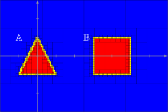
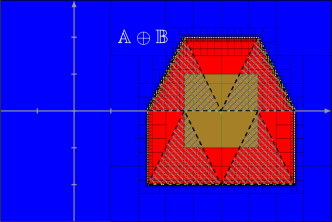
Figure 6: Minkowski sum of a square $\mathbb{B}$ and a triangle $\mathbb{A}$ computed using set membership algorithm.

5 Localization in an unstructured environment

Consider a robot $\mathcal{R}$ at position $\mathbf{p}=(p_{1},p_{2})$ in an unstructured environment described by the set $\mathbb{M}$. We assume that the heading $\theta$ of $\mathcal{R}$ is known with a good accuracy (for instance, by using a compass) and doesn’t need to be estimated. The robot is equipped several sonars which return the distance between the robot and the map with respect to the emission cone of the sonar. This section deals with the localization of the robots using the set-to-set transform. Several authors have already studied this problem using interval analysis [13, 14, 4] but in an environment made with segments.

Each sensor emits an acoustic wave in its direction $\alpha_{i}$ which propagates inside a cone of half angle $\gamma$ corresponding to the aperture of the beam. By measuring the time lag between the emission and the reception of the wave, reflected by the map, an interval $[d_{i}]=[d_{i}^{-},d_{i}^{+}]$ contains the true distance $d_{i}$ to the nearest obstacle which lies in the scope of the sensor can be obtained. The situation is depicted in Figure 7a. The area swept by the wave between $0$ and $d_{i}$ is free of obstacles whereas the map is hit by the wave at distance $d_{i}$. Define

$$\begin{array}[]{ccc}\mathbb{S}_{i}&=&\{(x,y)\mid x^{2}+y^{2}<d_{i}^{-}\text{ and }atan2(y,x)\in[\alpha_{i}-\gamma,\alpha_{i}+\gamma]\}\\ \Delta\mathbb{S}_{i}&=&\{(x,y)\mid x^{2}+y^{2}\in[d_{i}]\text{ and }atan2(y,x)\in[\alpha_{i}-\gamma,\alpha_{i}+\gamma]\}\end{array}$$

The set $\mathbb{S}_{i}$ is called the free sector and $\Delta\mathbb{S}_{i}$ is called the impact pie. These sets are depicted on Figure 7b.

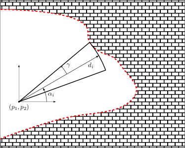
(a) Emission cone.

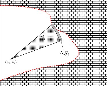
(b) The free sector $\mathbb{S}_{i}$ is represented by the dotted area while the gray pie $\Delta\mathbb{S}_{i}$ contains the impact point.

Figure 7: Sensor model used by the robot.

The set of all feasible positions $\mathbb{P}$ consistent with $[d_{i}]$ is

$$\mathbb{P}(i) =\{\mathbf{p}\in\mathbb{R}^{2}\mid(\mathbf{p}+\mathbb{S}_{i})\subset\mathbb{M}\text{ and }(\mathbf{p}+\Delta\mathbb{S}_{i})\cap\overline{\mathbb{M}}\neq\emptyset\}$$ (35)

$$=(\mathbb{M}\ominus\mathbb{S}_{i})\cap(\mathbb{\overline{M}}\oplus-\Delta\mathbb{S}_{i}).$$

With several measurements $[d_{i}]$ the set of all positions consistent with all data is

$$\mathbb{P} =\bigcap_{i}(\mathbb{M}\ominus\mathbb{S}_{i})\cap(\mathbb{\overline{M}}\oplus-\Delta\mathbb{S}_{i}).$$ (36)

Denote by $\mathcal{S}_{\mathbb{M}}$,$\mathcal{S}_{\mathbb{S}_{i}}$,$\mathcal{S}_{\Delta\mathbb{S}_{i}}$ separators for $\mathbb{M}$,$\mathbb{S}_{i}$ ,$\Delta\mathbb{S}_{i}$. Then a separator for $\mathbb{P}$ is

$$\mathcal{S}_{\mathbb{P}}=\bigcap_{i}(\mathcal{S}_{\mathbb{M}}\ominus\mathcal{S}_{\mathbb{S}_{i}})\cap(\overline{\mathcal{S}_{\mathbb{M}}}\oplus-\mathcal{S}_{\Delta\mathbb{S}_{i}}).$$ (37)

As an illustration, consider the situation described by Figure 8 (left), where a robot collects 6 sonar data. The width of the intervals corresponding to the range measurement is $\pm 1m$ .The first measurement corresponding to $i=1$ is painted green. Figure 8 (right) corresponds to an approximation of the set $\mathbb{M}\ominus\mathbb{S}_{1}$, obtained using a paver with the separator $\mathcal{S}_{\mathbb{M}}\ominus\mathcal{S}_{\mathbb{S}_{1}}$.

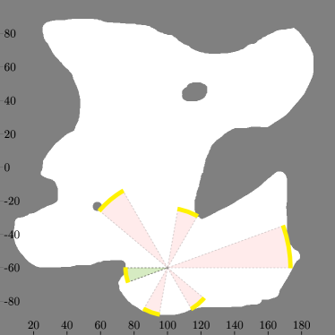
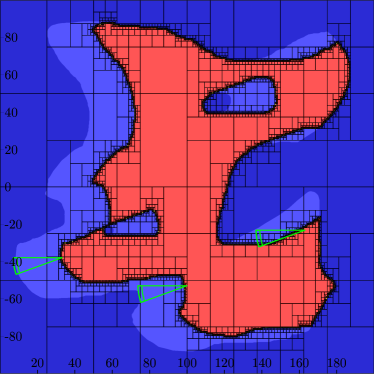
Figure 8: Left: a robot which collects 6 sonar range measurements. All free sectors $\mathbb{S}_{i}$ are included in the map $\mathbb{M}$ (in white) and the impact pies $\Delta\mathbb{S}_{i}$, in yellow intersects $\mathbb{\overline{M}}$. Right: Set of all positions for the robot consistent with the fact that the free sector $\mathbb{S}_{1}$ is inside $\mathbb{M}$.

Figure 9 (left) corresponds to an approximation of the set $\mathbb{\overline{M}}\oplus-\Delta\mathbb{S}_{1}$, obtained using a paver with the separator $\overline{\mathcal{S}_{\mathbb{M}}}\oplus-\mathcal{S}_{\Delta\mathbb{S}_{1}}$. It corresponds to the set of positions for the robot such that the impact pie $\Delta\mathbb{S}_{1}$ intersects the outside of the map $\mathbb{M}$. Figure 9 (right) corresponds to the set $(\mathbb{M}\ominus\mathbb{S}_{1})\cap(\mathbb{\overline{M}}\oplus-\Delta\mathbb{S}_{1}),$ i.e., it contains the position consistent with both $\Delta\mathbb{S}_{1}$ and $\mathbb{S}_{1}$.

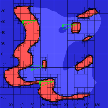
Figure 9: Left: Positions for the robot consistent with the impact pie $\Delta\mathbb{S}_{1}$. Right: Positions consistent with the free sector $\mathbb{S}_{1}$ and the impact pie $\Delta\mathbb{S}_{1}$.

Figure 10 (left) corresponds to an approximation of the set $\mathbb{P}$, obtained using a paver on with the separator $\mathcal{S}_{\mathbb{P}}$. It corresponds to the set of positions for the robot that all six impact pies $\Delta\mathbb{S}_{i}$ intersect the outside of the map $\mathbb{M}$ and all six free sectors are inside $\mathbb{M}$. A zoom of the solution set is given in Figure 10 (right). The computing time is 127 sec. and 205 boxes have been generated. Note that obtaining an inner approximation of the solution set was not possible using existing approaches that are not based on separators.

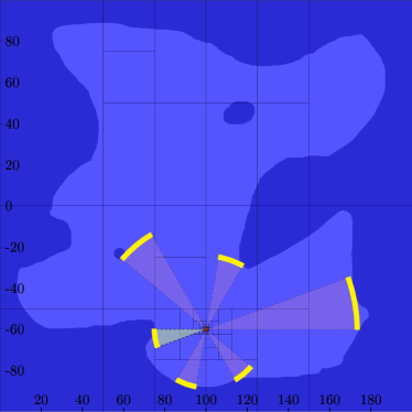
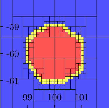
Figure 10: Left: Set of positions $\mathbb{P}$ for the robot consistent with all six free sectors $\mathbb{S}_{i}$ and all impact pies $\Delta\mathbb{S}_{i}$. Right: zoom around the solution set $\mathbb{P}$.

6 Conclusion

Separator-based techniques are particularly attractive when solving engineering applications, due to the fact that they can handle and propagate uncertainties in a context where the equations of the problem are non-linear and non-convex. Now, the performances of paving methods are extremely sensitive to the accuracy of the separators but also by the uncertainty generated by the dependency effect induced by the separator algebra. Indeed, when a separator, associated to the same set, occurs several times in the separator expression, a pessimism is introduced. It is thus important to factorize subexpression with separators into a single one which is computed separately by a specific algorithm. Another possibility is to rewrite the set expression in order to avoid multioccurences. This is what we have done for the Minkowski sum $\mathbb{A}\oplus\mathbb{B}$ and difference $\mathbb{A}\ominus\mathbb{B}$.

The efficiency of these new operators and their ability to get an inner and outer approximation of the solution set was illustrated on the problem of the localization of a robot.

References

- [1]
- [2] Frédéric Benhamou, Frédéric Goualard, Laurent Granvilliers & Jean-François Puget (1999): Revising Hull and Box Consistency. In: Proceedings of the 1999 International Conference on Logic Programming, Massachusetts Institute of Technology, Cambridge, MA, USA, pp. 230–244. Available at http://dl.acm.org/citation.cfm?id=341176.341208.
- [3] G. Chabert & L. Jaulin (2009): Contractor Programming. Artificial Intelligence 173, pp. 1079–1100, 10.1016/j.artint.2009.03.002.
- [4] E. Colle & Galerne (2013): Mobile robot localization by multiangulation using set inversion. Robotics and Autonomous Systems 61(1), pp. 39–48, 10.1016/j.robot.2012.09.006.
- [5] V. Drevelle & P. Bonnifait (2012): iGPS: Global Positioning in Urban Canyons with Road Surface Maps. IEEE Intelligent Transportation Systems Magazine 4(3), pp. 6–18, 10.1109/MITS.2012.2203222.
- [6] E. R. Hansen (1992): Bounding the solution of interval linear equations. SIAM Journal on Numerical Analysis 29(5), pp. 1493–1503, 10.1137/0729086.
- [7] L. Jaulin & B. Desrochers (2014): Introduction to the Algebra of Separators with Application to Path Planning. Engineering Applications of Artificial Intelligence 33, pp. 141–147, 10.1016/j.engappai.2014.04.010.
- [8] L. Jaulin, M. Kieffer, O. Didrit & E. Walter (2001): Applied Interval Analysis, with Examples in Parameter and State Estimation, Robust Control and Robotics. Springer-Verlag, London, 10.1007/978-1-4471-0249-6.
- [9] L. Jaulin, M. Kieffer, E. Walter & D. Meizel (2002): Guaranteed Robust Nonlinear Estimation with Application to Robot Localization. IEEE Transactions on systems, man and cybernetics; Part C Applications and Reviews 32(4), pp. 374–382, 10.1109/TSMCC.2002.806747.
- [10] L. Jaulin, E. Walter, O. Lévêque & D. Meizel (2000): Set Inversion for Chi-Algorithms, with Application to Guaranteed Robot Localization. Mathematics and Computers in Simulation 52(3-4), pp. 197–210, 10.1016/S0378-4754(00)00150-6.
- [11] R. B. Kearfott & V. Kreinovich, editors (1996): Applications of Interval Computations. Kluwer, Dordrecht, the Netherlands, 10.1007/978-1-4613-3440-8.
- [12] Michel Kieffer, Luc Jaulin, Eric Walter & Dominique Meizel (1999): Guaranteed mobile robot tracking using interval analysis. In: MISC’99, Workshop on Application of Interval Analysis to System and Control, Girona, Spain, pp. 347–360. Available at https://hal.archives-ouvertes.fr/hal-00844601.
- [13] Olivier Leveque, Luc Jaulin, Dominique Meizel & Eric Walter (1997): Vehicle localization from inaccurate telemetric data: a set inversion approach. In: 5th IFAC Symposium on Robot Control SY.RO.CO.’97, 1, Nantes, France, pp. 179–186. Available at https://hal.archives-ouvertes.fr/hal-00844041.
- [14] D. Meizel, O. Lévêque, L. Jaulin & E. Walter (2002): Initial Localization by Set Inversion. IEEE transactions on robotics and Automation 18(6), pp. 966–971, 10.1109/TRA.2002.805664.
- [15] R. E. Moore (1966): Interval Analysis. Prentice-Hall, Englewood Cliffs, NJ, 10.1126/science.158.3799.365.
- [16] L. Najman & H. Talbot (Eds) (1000): Mathematical morphology: from theory to applications. ISTE-Wiley, 10.1002/9781118600788.
- [17] Kenji Shoji (1991): Quadtree decomposition of binary structuring elements. In: Nonlinear Image Processing II, Proc. SPIE 1451, 10.1117/12.44322.
- [18] J. Sliwka, F. Le Bars, O. Reynet & L. Jaulin (2011): Using interval methods in the context of robust localization of underwater robots. In: NAFIPS 2011, El Paso, USA, 10.1109/NAFIPS.2011.5751922.
- [19] W. Taha & A. Duracz (2015): Acumen: An Open-source Testbed for Cyber-Physical Systems Research. In: CYCLONE’15, 10.1007/978-3-319-47063-4_11.