Control Synthesis of Nonlinear Sampled Switched Systems using Euler’s Method

Abstract

In this paper, we propose a symbolic control synthesis method for nonlinear sampled switched systems whose vector fields are one-sided Lipschitz. The main idea is to use an approximate model obtained from the forward Euler method to build a guaranteed control. The benefit of this method is that the error introduced by symbolic modeling is bounded by choosing suitable time and space discretizations. The method is implemented in the interpreted language Octave. Several examples of the literature are performed and the results are compared with results obtained with a previous method based on the Runge-Kutta integration method.

1 Introduction

As said in [11], in the methods of symbolic analysis and control of hybrid systems, the way of representing sets of state values and computing reachable sets for systems defined by ordinary differential equations (ODEs) is fundamental (see, e.g., [3, 15]). An interesting approach appeared recently, based on the propagation of reachable sets using guaranteed Runge-Kutta methods with adaptive step size control (see [7, 18]). In [11] such guaranteed integration methods are used in the framework of sampled switched systems.

Given an ODE of the form $\dot{x}(t)=f(t,x(t))$, and a set of initial values $X_{\_}0$, a symbolic (or “set-valued”) integration method consists in computing a sequence of approximations $(t_{\_}n,\tilde{x}_{\_}n)$ of the solution $x(t;x_{\_}0)$ of the ODE with $x_{\_}0\in X_{\_}0$ such that $\tilde{x}_{\_}n\approx x(t_{\_}n;x_{\_}{n-1})$. Symbolic integration methods extend classical numerical integration methods which correspond to the case where $X_{\_}0$ is just a singleton $\{x_{\_}0\}$. The simplest numerical method is Euler’s method in which $t_{\_}{n+1}=t_{\_}n+h$ for some step-size $h$ and $\tilde{x}_{\_}{n+1}=\tilde{x}_{\_}n+hf(t_{\_}n,\tilde{x}_{\_}n)$; so the derivative of $x$ at time $t_{\_}n$, $f(t_{\_}n,x_{\_}n)$, is used as an approximation of the derivative on the whole time interval. This method is very simple and fast, but requires small step-sizes $h$. More advanced methods coming from the Runge-Kutta family use a few intermediate computations to improve the approximation of the derivative. The general form of an explicit $s$-stage Runge-Kutta formula of the form $\tilde{x}_{\_}{n+1}=\tilde{x}_{\_}n+h\Sigma_{\_}{i=1}^{s}b_{\_}ik_{\_}i$ where $k_{\_}i=f(t_{\_}n+c_{\_}ih,\tilde{x}_{\_}n+h\Sigma_{\_}{j=1}^{i-1}a_{\_}{ij}k_{\_}j)$ for $i=2,3,...,s$. A challenging question is then to compute a bound on the distance between the true solution and the numerical solution, i.e.: $\|x(t_{\_}n;x_{\_}{n-1})-x_{\_}n\|$. This distance is associated to the local truncation error of the numerical method. In [11], such a bound is computed using the Lagrange remainders of Taylor expansions. This is achieved using affine arithmetic [28] (by application of the Banach’s fixpoint theorem and Picard-Lindelöf operator, see [24]). In the end, the Runge-Kutta based method of [11] is an elaborated method that requires the use of affine arithmetic, Picard iteration and computation of Lagrange remainder.

In contrast, in this paper, we use ordinary arithmetic (instead of affine arithmetic) and a basic Euler scheme (instead of Runge-Kutta schemes). We need neither estimate Lagrange remainders nor perform Picard iteration in combination with Taylor series. Our simple Euler-based approach is made possible by having recourse to the notion of one-sided Lipschitz (OSL) function [13]. This allows us to bound directly the global error, i.e. the distance between the approximate point $\tilde{x}(t)$ computed by the Euler scheme and the exact solution $x(t)$ for all $t\geq 0$ (see Theorem 1).

Plan. In Section 2, we give details on related work. In Section 3, we state our main result that bounds the global error introduced by the Euler scheme in the context of systems with OSL flows. In Section 4, we explain how to apply this result to the synthesis of symbolic control of sampled switched systems. We give numerical experiments and results in Section 5 for five exampes of the literature, and compare them with results obtained with the method of [11]. We give final remarks in Section 6.

2 Related work

Most of the recent work on the symbolic (or set-valued) integration of nonlinear ODEs is based on the upper bounding of the Lagrange remainders either in the framework of Taylor series or Runge-Kutta schemes [3, 6, 7, 9, 10, 11, 21, 25, 27]. Sets of states are generally represented as vectors of intervals (or “rectangles”) and are manipulated through interval arithmetic [23] or affine arithmetic [28]. Taylor expansions with Lagrange remainders are also used in the work of [3], which uses “polynomial zonotopes” for representing sets of states in addition to interval vectors. None of these works uses the Euler scheme nor the notion of one-sided Lipschitz constant.

In the literature on symbolic integration, the Euler scheme with OSL conditions is explored in [13, 19]. Our approach is similar but establishes an analytical result for the global error of Euler’s estimate (see Theorem 1) rather than analyzing, in terms of complexity, the speed of convergence to zero, the accuracy and the stability of Euler’s method.

In the control literature, OSL conditions have been recently applied to control and stabilization [2, 8], but do not make use of Euler’s method. To our knowledge, our work applies for the first time Euler’s scheme with OSL conditions to the symbolic control of hybrid systems.

3 Sampled switched systems with OSL conditions

3.1 Control of switched systems

Let us consider the nonlinear switched system

$$\dot{x}(t)=f_{\_}{\sigma(t)}(x(t))$$ (1)

defined for all $t\geq 0$, where $x(t)\in\mathbb{R}^{n}$ is the state of the system, $\sigma(\cdot):\mathbb{R}^{+}\longrightarrow U$ is the switching rule. The finite set $U=\{1,\dots,N\}$ is the set of switching modes of the system. We focus on sampled switched systems: given a sampling period $\tau>0$, switchings will occur at times $\tau$, $2\tau$, … The switching rule $\sigma(\cdot)$ is thus constant on the time interval $[(k-1)\tau,k\tau)$ for $k\geq 1$. For all $j\in U$, $f_{\_}j$ is a function from $\mathbb{R}^{n}$ to $\mathbb{R}^{n}$. We make the following hypothesis:

$$(H0)\quad\mbox{ For all $j\in U$, $f_{\_}j$ is a locally Lipschitz continuous map}.$$

As in [16], we make the assumption that the vector field $f_{\_}j$ is such that the solutions of the differential equation (1) are defined, e.g. by assuming that the support of the vector field $f_{\_}j$ is compact. We will denote by $\phi_{\_}\sigma(t;x^{0})$ the solution at time $t$ of the system:

$$\dot{x}(t) =f_{\_}{\sigma(t)}(x(t)),$$ (2)

$$x(0) =x^{0}.$$

Often, we will consider $\phi_{\_}\sigma(t;x^{0})$ on the interval $0\leq t<\tau$ for which $\sigma(t)$ is equal to a constant, say $j\in U$. In this case, we will abbreviate $\phi_{\_}\sigma(t;x^{0})$ as $\phi_{\_}j(t;x^{0})$. We will also consider $\phi_{\_}\sigma(t;x^{0})$ on the interval $0\leq t<k\tau$ where $k$ is a positive integer, and $\sigma(t)$ is equal to a constant, say $j_{\_}{k^{\prime}}$, on each interval $[(k^{\prime}-1)\tau,k^{\prime}\tau)$ with $1\leq k^{\prime}\leq k$; in this case, we will abbreviate $\phi_{\_}\sigma(t;x^{0})$ as $\phi_{\_}\pi(t;x^{0})$, where $\pi$ is a sequence of $k$ modes (or “pattern”) of the form $\pi=j_{\_}1\cdot j_{\_}2\cdot\dots\cdot j_{\_}k$.

We will assume that $\phi_{\_}\sigma$ is continuous at time $k\tau$ for all positive integer $k$. This means that there is no “reset” at time $k^{\prime}\tau$ ($1\leq k^{\prime}\leq k$); the value of $\phi_{\_}\sigma(t,x^{0})$ for $t\in[(k^{\prime}-1)\tau,k\tau]$ corresponds to the solution of $\dot{x}(u)=f_{\_}{j_{\_}{k^{\prime}}}(x(u))$ for $u\in[0,\tau]$ with initial value $\phi_{\_}\sigma((k^{\prime}-1)\tau;x^{0})$.

Given a “recurrence set” $R\subset\mathbb{R}^{n}$ and a “safety set” $S\subset\mathbb{R}^{n}$ which contains $R$ ($R\subseteq S$), we are interested in the synthesis of a control such that: starting from any initial point $x\in R$, the controlled trajectory always returns to $R$ within a bounded time while never leaving $S$. We suppose that sets $R$ and $S$ are compact. Furthermore, we suppose that $S$ is convex.

We denote by $T$ a compact overapproximation of the image by $\phi_{\_}j$ of $S$ for $0\leq t\leq\tau$ and $j\in U$, i.e. $T$ is such that

$$T\supseteq\{\phi_{\_}j(t;x^{0})\ |\ j\in U,0\leq t\leq\tau,x^{0}\in S\}.$$

The existence of $T$ is guaranteed by assumption $(H0)$. We know furthermore by $(H0)$ that, for all $j\in U$, there exists a constant $L_{\_}j>0$ such that:

$$\|f_{\_}j(y)-f_{\_}j(x)\|\leq L_{\_}j\,\|y-x\|\quad\forall x,y\in S.$$ (3)

Let us define $C_{\_}j$ for all $j\in U$:

$$C_{\_}j=\sup_{\_}{x\in S}\ L_{\_}j\|f_{\_}j(x)\|\quad\text{for all}\quad j\in U.$$ (4)

We make the additional hypothesis that the mappings $f_{\_}j$ are one-sided Lipschitz (OSL) [13]. Formally:

$$(H1)\quad\mbox{ For all $j\in U$, there exists a constant $\lambda_{\_}j\in\mathbb{R}$ such that}$$

$$\langle f_{\_}j(y)-f_{\_}j(x),y-x\rangle\leq\lambda_{\_}j\,\|y-x\|^{2}\quad\forall x,y\in T,$$

where $\langle\cdot,\cdot\rangle$ denotes the scalar product of two vectors of $\mathbb{R}^{n}$.

Remark 1.

Constants $\lambda_{\_}j$, $L_{\_}j$ and $C_{\_}j$ ($j\in U$) can be computed using (constrained) optimization algorithms. See Section 5 for details.

3.2 Euler approximate solutions

Given an initial point $\tilde{x}^{0}\in S$ and a mode $j\in U$, we define the following “linear approximate solution” $\tilde{\phi}_{\_}j(t;\tilde{x}^{0})$ for $t$ on $[0,\tau]$ by:

$$\tilde{\phi}_{\_}j(t;\tilde{x}^{0})=\tilde{x}^{0}+tf_{\_}j(\tilde{x}^{0}).$$ (5)

Note that formula (5) is nothing else but the explicit forward Euler scheme with “time step” $t$. It is thus a consistent approximation of order $1$ in $t$ of the exact solution of (1) under the hypothesis $\tilde{x}^{0}=x^{0}$.

More generally, given an initial point $\tilde{x}^{0}\in S$ and pattern $\pi$ of $U^{k}$, we can define a “(piecewise linear) approximate solution” $\tilde{\phi}_{\_}\pi(t;\tilde{x}^{0})$ of $\phi_{\_}\pi$ at time $t\in[0,k\tau]$ as follows:

• $\tilde{\phi}_{\_}\pi(t;\tilde{x}^{0})=tf_{\_}j(\tilde{x}^{0})+\tilde{x}^{0}$ if $\pi=j\in U$, $k=1$ and $t\in[0,\tau]$, and

• $\tilde{\phi}_{\_}{\pi}(k\tau+t;\tilde{x}^{0})=tf_{\_}j(\tilde{z})+\tilde{z}$ with $\tilde{z}=\tilde{\phi}_{\_}{\pi^{\prime}}((k-1)\tau;\tilde{x}^{0})$, if $k\geq 2$, $t\in[0,\tau]$, $\pi=j\cdot\pi^{\prime}$ for some $j\in U$ and $\pi^{\prime}\in U^{k-1}$.

We wish to synthesize a guaranteed control $\sigma$ for $\phi_{\_}{\sigma}$ using the approximate functions $\tilde{\phi}_{\_}\pi$.We define the closed ball of center $x\in\mathbb{R}^{n}$ and radius $r>0$, denoted $B(x,r)$, as the set $\{x^{\prime}\in\mathbb{R}^{n}\ |\ \|x^{\prime}-x\|\leq r\}$.

Given a positive real $\delta$, we now define the expression $\delta_{\_}j(t)$ which, as we will see in Theorem 1, represents (an upper bound on) the error associated to $\tilde{\phi}_{\_}j(t;\tilde{x}^{0})$ (i.e. $\|\tilde{\phi}_{\_}j(t;\tilde{x}^{0})-\phi_{\_}j(t;x^{0})\|$).

Definition 1.

Let $\delta$ be a positive constant. Let us define, for all $0\leq t\leq\tau$, $\delta_{\_}j(t)$ as follows:

• if $\lambda_{\_}j<0$:

  $$\delta_{\_}j(t)=\left(\delta^{2}e^{\lambda_{\_}jt}+\frac{C_{\_}j^{2}}{\lambda_{\_}j^{2}}\left(t^{2}+\frac{2t}{\lambda_{\_}j}+\frac{2}{\lambda_{\_}j^{2}}\left(1-e^{\lambda_{\_}jt}\right)\right)\right)^{\frac{1}{2}}$$

• if $\lambda_{\_}j=0:$

  $$\delta_{\_}j(t)=\left(\delta^{2}e^{t}+C_{\_}j^{2}(-t^{2}-2t+2(e^{t}-1))\right)^{\frac{1}{2}}$$

• if $\lambda_{\_}j>0:$

  $$\delta_{\_}j(t)=\left(\delta^{2}e^{3\lambda_{\_}jt}+\frac{C_{\_}j^{2}}{3\lambda_{\_}j^{2}}\left(-t^{2}-\frac{2t}{3\lambda_{\_}j}+\frac{2}{9\lambda_{\_}j^{2}}\left(e^{3\lambda_{\_}jt}-1\right)\right)\right)^{\frac{1}{2}}$$

Note that $\delta_{\_}j(t)=\delta$ for $t=0$. The function $\delta_{\_}j(\cdot)$ depends implicitly on two parameters: $\delta\in\mathbb{R}$ and $j\in U$. In Section 4, we will use the notation $\delta^{\prime}_{\_}j(\cdot)$ where the parameters are denoted by $\delta^{\prime}$ and $j$.

Theorem 1.

Given a sampled switched system satisfying (H0-H1), consider a point $\tilde{x}^{0}$ and a positive real $\delta$. We have, for all $x^{0}\in B(\tilde{x}^{0},\delta)$, $t\in[0,\tau]$ and $j\in U$:

$\phi_{\_}j(t;x^{0})\in B(\tilde{\phi}_{\_}j(t;\tilde{x}^{0}),\delta_{\_}j(t))$.

Proof.

Consider on $t\in[0,\tau]$ the differential equations

$$\frac{dx(t)}{dt}=f_{\_}j(x(t))$$

and

$$\frac{d\tilde{x}(t)}{dt}=f_{\_}j(\tilde{x}^{0}).$$

with initial points $x^{0}\in S,\tilde{x}^{0}\in S$ respectively. We will abbreviate $\phi_{\_}j(t;x^{0})$ (resp. $\tilde{\phi}_{\_}j(t;\tilde{x}^{0})$) as $x(t)$ (resp. $\tilde{x}(t)$). We have

$$\frac{d}{dt}(x(t)-\tilde{x}(t))=\left(f_{\_}j(x(t))-f_{\_}j(\tilde{x}^{0})\right),$$

then

$$\frac{1}{2}\,\frac{d}{dt}(\|x(t)-\tilde{x}(t)\|^{2}) = \left\langle f_{\_}j(x(t))-f_{\_}j(\tilde{x}^{0}),x(t)-\tilde{x}(t)\right\rangle$$

$$= \left\langle f_{\_}j(x(t))-f_{\_}j(\tilde{x}(t))+f_{\_}j(\tilde{x}(t))-f_{\_}j(\tilde{x}^{0}),x(t)-\tilde{x}(t)\right\rangle$$

$$= \left\langle f_{\_}j(x(t))-f_{\_}j(\tilde{x}(t)),x(t)-\tilde{x}(t)\right\rangle+\left\langle f_{\_}j(\tilde{x}(t))-f_{\_}j(\tilde{x}^{0}),x(t)-\tilde{x}(t)\right\rangle$$

$$\leq \left\langle f_{\_}j(x(t))-f_{\_}j(\tilde{x}(t)),x(t)-\tilde{x}(t)\right\rangle+\|f_{\_}j(\tilde{x}(t))-f_{\_}j(\tilde{x}^{0})\|\|x(t)-\tilde{x}(t)\|.$$

The last expression has been obtained using the Cauchy-Schwarz inequality. Using $(H1)$ and (3), we have

$$\frac{1}{2}\,\frac{d}{dt}(\|x(t)-\tilde{x}(t)\|^{2}) \leq \lambda_{\_}j\|x(t)-\tilde{x}(t)\|^{2}+\,\|f_{\_}j(\tilde{x}(t))-f_{\_}j(\tilde{x}^{0})\|\,\|x(t)-\tilde{x}(t)\|$$

$$\leq \lambda_{\_}j\|x(t)-\tilde{x}(t)\|^{2}+L_{\_}j\,\|\tilde{x}(t)-\tilde{x}^{0}\|\,\|x(t)-\tilde{x}(t)\|$$

$$\leq \lambda_{\_}j\|x(t)-\tilde{x}(t)\|^{2}+L_{\_}jt\,\|f_{\_}j(\tilde{x}^{0})\|\,\|x(t)-\tilde{x}(t)\|.$$

Using (4) and a Young inequality, we then have

$$\frac{1}{2}\,\frac{d}{dt}(\|x(t)-\tilde{x}(t)\|^{2}) \leq \lambda_{\_}j\|x(t)-\tilde{x}(t)\|^{2}+C_{\_}j\,t\,\|x(t)-\tilde{x}(t)\|$$

$$\leq \lambda_{\_}j\|x(t)-\tilde{x}(t)\|^{2}+C_{\_}j\,t\,\frac{1}{2}\left(\alpha\|x(t)-\tilde{x}(t)\|^{2}+\frac{1}{\alpha}\right)$$

for all $\alpha>0$.

• In the case $\lambda_{\_}j<0$:

  For $t>0$, we choose $\alpha>0$ such that $C_{\_}jt\alpha=-\lambda_{\_}j$, i.e. $\alpha=-\frac{\lambda_{\_}j}{C_{\_}j\,t}$. It follows, for all $t\in[0,\tau]$:

  $$\frac{1}{2}\,\frac{d}{dt}(\|x(t)-\tilde{x}(t)\|^{2})\leq\frac{\lambda_{\_}j}{2}\|x(t)-\tilde{x}(t)\|^{2}-\frac{C_{\_}jt}{2\alpha}=\frac{\lambda_{\_}j}{2}\|x(t)-\tilde{x}(t)\|^{2}-\frac{(C_{\_}jt)^{2}}{2\lambda_{\_}j}.$$

  We thus get:

  $$\|x(t)-\tilde{x}(t)\|^{2}\leq\|x^{0}-\tilde{x}^{0}\|^{2}\,e^{\lambda_{\_}jt}+\frac{C_{\_}j^{2}}{\lambda_{\_}j^{2}}\left(t^{2}+\frac{2t}{\lambda_{\_}j}+\frac{2}{\lambda_{\_}j^{2}}\left(1-e^{\lambda_{\_}jt}\right)\right).$$

• In the case $\lambda_{\_}j>0$:

  For $t>0$, we choose $\alpha>0$ such that $C_{\_}jt\alpha=\lambda_{\_}j$, i.e. $\alpha=\frac{\lambda_{\_}j}{C_{\_}j\,t}$. It follows, for all $t\in[0,\tau]$:

  $$\frac{1}{2}\,\frac{d}{dt}(\|x(t)-\tilde{x}(t)\|^{2})\leq\frac{3\lambda_{\_}j}{2}\|x(t)-\tilde{x}(t)\|^{2}+\frac{C_{\_}jt}{2\alpha}=\frac{3\lambda_{\_}j}{2}\|x(t)-\tilde{x}(t)\|^{2}+\frac{(C_{\_}jt)^{2}}{2\lambda_{\_}j}.$$

  We thus get:

  $$\|x(t)-\tilde{x}(t)\|^{2}\leq\|x^{0}-\tilde{x}^{0}\|^{2}\,e^{3\lambda_{\_}jt}+\frac{C_{\_}j^{2}}{3\lambda_{\_}j^{2}}\left(-t^{2}-\frac{2t}{3\lambda_{\_}j}+\frac{2}{9\lambda_{\_}j^{2}}\left(e^{3\lambda_{\_}jt}-1\right)\right)$$

• In the case $\lambda_{\_}j=0$:

  For $t>0$, we choose $\alpha=\frac{1}{C_{\_}jt}$. It follows:

  $$\frac{d}{dt}(\|x(t)-\tilde{x}(t)\|^{2})\leq\|x(t)-\tilde{x}(t)\|^{2}+C_{\_}jt^{2}$$

  We thus get:

  $$\|x(t)-\tilde{x}(t)\|^{2}\leq\|x^{0}-\tilde{x}^{0}\|^{2}e^{t}+C_{\_}j^{2}(-t^{2}-2t+2(e^{t}-1))$$

  In every case, since by hypothesis $x^{0}\in B(\tilde{x}^{0},\delta)$ (i.e. $\|x^{0}-\tilde{x}^{0}\|^{2}\leq\delta^{2}$), we have, for all $t\in[0,\tau]$:

  $$\|x(t)-\tilde{x}(t)\|\leq\delta_{\_}j(t).$$

It follows: $\phi_{\_}j(t;x^{0})\in B(\tilde{\phi}_{\_}j(t;\tilde{x}^{0}),\delta)$ for $t\in[0,\tau]$.

∎

Remark 2.

In Theorem 1, we have supposed that the step size $h$ used in Euler’s method was equal to the sampling period $\tau$ of the switching system. Actually, in order to have better approximations, it is often convenient to take a fraction of $\tau$ as for $h$ (e.g., $h=\frac{\tau}{10}$). Such a splitting is called “sub-sampling” in numerical methods. See Section 5 for details.

Corollary 1.

Given a sampled switched system satisfying (H0-H1), consider a point $\tilde{x}^{0}\in S$, a real $\delta>0$ and a mode $j\in U$ such that:

1. $B(\tilde{x}^{0},\delta)\subseteq S$,

2. $B(\tilde{\phi}_{\_}j(\tau;\tilde{x}^{0}),\delta_{\_}j(\tau))\subseteq S$, and

3. $\frac{d^{2}(\delta_{\_}j(t))}{dt^{2}}>0$ for all $t\in[0,\tau]$.

Then we have, for all $x^{0}\in B(\tilde{x}^{0},\delta)$ and $t\in[0,\tau]$: $\phi_{\_}j(t;x^{0})\in S$.

Proof.

By items 1 and 2, $B(\tilde{\phi}_{\_}j(t;\tilde{x}^{0}),\delta_{\_}j(t))$ for $t=0$ and $t=\tau$. Since $\delta_{\_}j(\cdot)$ is convex on $[0,\tau]$ by item 3, and $S$ is convex, we have $B(\tilde{\phi}_{\_}j(t;\tilde{x}^{0}),\delta_{\_}j(t))\subseteq S$ for all $t\in[0,\tau]$. It follows from Theorem 1 that $\phi_{\_}j(t;x^{0})\in B(\tilde{\phi}_{\_}j(t;\tilde{x}^{0}),\delta_{\_}j(t))\subseteq S$ for all $1\leq t\leq\tau$. ∎

Remark 3.

Condition 3 of Corollary 1 on the convexity of $\delta_{\_}j(\cdot)$ on $[0,\tau]$ can be established again using an optimization function (see Section 5).

4 Application to control synthesis

Consider a point $\tilde{x}^{0}\in S$, a positive real $\delta$ and a pattern $\pi$ of length $k$. Let $\pi(k^{\prime})$ denote the $k^{\prime}$-th element (mode) of $\pi$ for $1\leq k^{\prime}\leq k$. Let us abbreviate the $k^{\prime}$-th approximate point $\tilde{\phi}_{\_}{\pi}(k^{\prime}\tau;\tilde{x}^{0})$ as $\tilde{x}_{\_}\pi^{k^{\prime}}$ for $k^{\prime}=1,...,k$, and let $\tilde{x}_{\_}\pi^{k^{\prime}}=\tilde{x}^{0}$ for $k^{\prime}=0$. It is easy to show that $\tilde{x}_{\_}\pi^{k^{\prime}}$ can be defined recursively for $k^{\prime}=1,...,k$, by: $\tilde{x}_{\_}\pi^{k^{\prime}}=\tilde{x}_{\_}\pi^{k^{\prime}-1}+\tau f_{\_}{j}(\tilde{x}_{\_}\pi^{k^{\prime}-1})$ with $j=\pi(k^{\prime})$.

Let us now denote by $\delta_{\_}\pi^{k^{\prime}}$ (an upper bound on) the error associated to $\tilde{x}_{\_}\pi^{k^{\prime}}$, i.e. $\|\tilde{x}_{\_}\pi^{k^{\prime}}-\phi_{\_}\pi(k^{\prime}\tau;x^{0})\|$. Using repeatedly Theorem 1, $\delta_{\_}{\pi}^{k^{\prime}}$ can be defined recursively as follows:

For $k^{\prime}=0$: $\delta_{\_}{\pi}^{k^{\prime}}=\delta$, and for $1\leq k^{\prime}\leq k$: $\delta^{k^{\prime}}_{\_}{\pi}=\delta^{\prime}_{\_}j(\tau)$ where $\delta^{\prime}$ denotes $\delta^{k^{\prime}-1}_{\_}{\pi}$, and $j$ denotes $\pi(k^{\prime})$.
Likewise, for $0\leq t\leq k\tau$, let us denote by $\delta_{\_}{\pi}(t)$ (an upper bound on) the global error associated to $\tilde{\phi}_{\_}\pi(t;\tilde{x}^{0})$ (i.e. $\|\tilde{\phi}_{\_}\pi(t;\tilde{x}^{0})-\phi_{\_}\pi(t;x^{0})\|$). Using Theorem 1, $\delta_{\_}{\pi}(t)$ can be defined itself as follows:

• for $t=0$: $\delta_{\_}\pi(t)=\delta$,

• for $0<t\leq k\tau$: $\delta_{\_}{\pi}(t)=\delta^{\prime}_{\_}{j}(t^{\prime})$ with $\delta^{\prime}=\delta_{\_}\pi^{\ell-1}$, $j=\pi(\ell)$, $t^{\prime}=t-(\ell-1)\tau$ and $\ell=\lceil\frac{t}{\tau}\rceil$.

Note that, for $0\leq k^{\prime}\leq k$, we have: $\delta_{\_}{\pi}(k^{\prime}\tau)=\delta_{\_}\pi^{k^{\prime}}$. We have:

Theorem 2.

Given a sampled switched system satisfying (H0-H1), consider a point $\tilde{x}^{0}\in S$, a positive real $\delta$ and a pattern $\pi$ of length $k$ such that, for all $1\leq k^{\prime}\leq k$:

1. $B(\tilde{x}_{\_}\pi^{k^{\prime}},\delta_{\_}{\pi}^{k^{\prime}})\subseteq S$ and

2. $\frac{d^{2}(\delta^{\prime}_{\_}j(t))}{dt^{2}}>0$ for all $t\in[0,\tau]$, with $j=\pi(k^{\prime})$ and $\delta^{\prime}=\delta_{\_}\pi^{k^{\prime}-1}$.

Then we have, for all $x^{0}\in B(\tilde{x}^{0},\delta)$ and $t\in[0,k\tau]$:  $\phi_{\_}{\pi}(t;x^{0})\in S$.

Proof.

By induction on $k$ using Corollary 1. ∎

The statement of Theorem 2 is illustrated in Figure 1 for $k=2$. From Theorem 2, it easily follows:

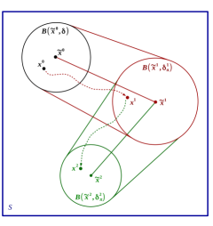
Figure 1: Illustration of Theorem 2.

Corollary 2.

Given a switched system satisfying (H0-H1), consider a positive real $\delta$ and a finite set of points $\tilde{x}_{\_}1,\dots\tilde{x}_{\_}m$ of $S$ such that all the balls $B(\tilde{x}_{\_}i,\delta)$ cover $R$ and are included into $S$ (i.e. $R\subseteq\bigcup_{\_}{i=1}^{m}B(\tilde{x}_{\_}i,\delta)\subseteq S$). Suppose furthermore that, for all $1\leq i\leq m$, there exists a pattern $\pi_{\_}i$ of length $k_{\_}i$ such that:

1. $B((\tilde{x}_{\_}i)_{\_}{\pi_{\_}i}^{k^{\prime}},\delta_{\_}{\pi_{\_}i}^{k^{\prime}})\subseteq S$, for all $k^{\prime}=1,\dots,k_{\_}i-1$

2. $B((\tilde{x}_{\_}i)_{\_}{\pi_{\_}i}^{k_{\_}i},\delta_{\_}{\pi_{\_}i}^{k_{\_}i})\subseteq R.$

3. $\frac{d^{2}(\delta^{\prime}_{\_}j(t))}{dt^{2}}>0$ with $j=\pi_{\_}i(k^{\prime})$ and $\delta^{\prime}=\delta_{\_}{\pi_{\_}i}^{k^{\prime}-1}$, for all $k^{\prime}\in\{1,...,k_{\_}i\}$ and $t\in[0,\tau]$.

These properties induce a control $\sigma$ which guarantees

• (safety): if $x\in R$, then $\phi_{\_}{\sigma}(t;x)\in S$ for all $t\geq 0$, and

• (recurrence): if $x\in R$ then $\phi_{\_}{\sigma}(k\tau;x)\in R$ for some $k\in\{k_{\_}1,\dots,k_{\_}m\}$.

Corollary 2 gives the theoretical foundations of the following method for synthesizing $\sigma$ ensuring recurrence in $R$ and safety in $S$:

• we (pre-)compute $\lambda_{\_}j,L_{\_}j,C_{\_}j$ for all $j\in U$;

• we find $m$ points $\tilde{x}_{\_}1,\dots\tilde{x}_{\_}m$ of $S$ and $\delta>0$ such that $R\subseteq\bigcup_{\_}{i=1}^{m}B(\tilde{x}_{\_}i,\delta)\subseteq S$;

• we find $m$ patterns $\pi_{\_}i$ ($i=1,...,m$) such that conditions 1-2-3 of Corollary 2 are satisfied.

A covering of $R$ with balls as stated in Corollary 2 is illustrated in Figure 2. The control synthesis method based on Corollary 2 is illustrated in Figure 3 (left) together with an illustration of method of [11] (right).

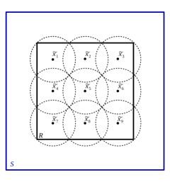
Figure 2: A set of balls covering $R$ and contained in $S$.

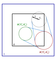
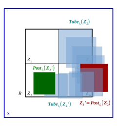
Figure 3: Control of ball $B(\tilde{x}_{\_}3,\delta)$ with our method (left); control of tile $Z_{\_}2$ with the method of [11] (right).

5 Numerical experiments and results

This method has been implemented in the interpreted language Octave, and the experiments performed on a 2.80 GHz Intel Core i7-4810MQ CPU with 8 GB of memory.

The computation of constants $L_{\_}j$, $C_{\_}j$, $\lambda_{\_}j$ ($j\in U$) are realized with a constrained optimization algorithm. They are performed using the “sqp” function of Octave, applied on the following optimization problems:

• Constant $L_{\_}j$:

  $$L_{\_}j=\max_{\_}{{x,y}\in S,\ x\neq y}\frac{\|f_{\_}j(y)-f_{\_}j(x)\|}{\|y-x\|}$$

• Constant $C_{\_}j$:

  $$C_{\_}j=\max_{\_}{{x}\in S}L_{\_}j\|f_{\_}j(x)\|$$

• Constant $\lambda_{\_}j$:

  $$\lambda_{\_}j=\max_{\_}{{x,y}\in T,\ x\neq y}\frac{\langle f_{\_}j(y)-f_{\_}j(x),y-x\rangle}{\|y-x\|^{2}}$$

Likewise, the convexity test $\frac{d^{2}(\delta^{\prime}_{\_}j(t))}{dt^{2}}>0$ can be performed similarly.

Note that in some cases, it is advantageous to use a time sub-sampling to compute the image of a ball. Indeed, because of the exponential growth of the radius $\delta_{\_}j(t)$ within time, computing a sequence of balls can lead to smaller ball images. It is particularly advantageous when a constant $\lambda_{\_}j$ is negative. We illustrate this with the example of the DC-DC converter. It has two switched modes, for which we have $\lambda_{\_}1=-0.014215$ and $\lambda_{\_}2=0.142474$. In the case $\lambda_{\_}j<0$, the associated formula $\delta_{\_}j(t)$ has the behavior of Figure 4 (a). In the case $\lambda_{\_}j>0$, the associated formula $\delta_{\_}j(t)$ has the behavior of Figure 4 (b). In the case $\lambda_{\_}j<0$, if the time sub-sampling is small enough, one can compute a sequence of balls with reducing radius, which makes the synthesis easier.

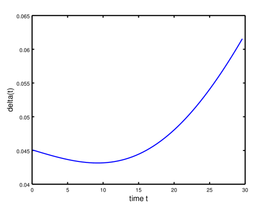
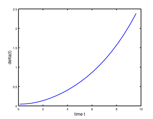
(a)	(b)

Figure 4: Behavior of $\delta_{\_}j(t)$ for the DC-DC converter with $\delta_{\_}j(0)=0.045$. (a) Evolution of $\delta_{\_}1(t)$ (with $\lambda_{\_}1<0$); (b) Evolution of $\delta_{\_}2(t)$ (with $\lambda_{\_}2>0$).

In the following, we give the results obtained with our Octave implementation of this Euler-based method on 5 examples, and compare them with those given by the C++ implementation DynIBEX [26] of the Runge-Kutta based method used in [11].

5.1 Four-room apartment

We describe a first application on a 4-room 16-switch building ventilation case study adapted from [22]. The model has been simplified in order to get constant parameters. The system is a four room apartment subject to heat transfer between the rooms, with the external environment, the underfloor, and human beings. The dynamics of the system is given by the following equation:

$$\frac{dT_{\_}i}{dt}=\sum_{\_}{j\in\mathcal{N}^{\text{*}}\setminus\{i\}}a_{\_}{ij}(T_{\_}j-T_{\_}i)+\delta_{\_}{s_{\_}i}b_{\_}i(T_{\_}{s_{\_}i}^{4}-T_{\_}i^{4})+c_{\_}i\max\left(0,\frac{V_{\_}i-V_{\_}i^{\text{*}}}{\bar{V_{\_}i}-V_{\_}i^{\text{*}}}\right)(T_{\_}u-T_{\_}i),\quad\mbox{for }i=1,...,4.$$

The state of the system is given by the temperatures in the rooms $T_{\_}i$, for $i\in\mathcal{N}=\{1,\dots,4\}$. Room $i$ is subject to heat exchange with different entities stated by the indices $\mathcal{N}^{\text{*}}=\{1,2,3,4,u,o,c\}$. We have $T_{\_}0=30,T_{\_}c=30,T_{\_}u=17$, $\delta_{\_}{s_{\_}i}=1$ for $i\in\mathcal{N}$. The (constant) parameters $T_{\_}{s_{\_}i}$, $V_{\_}i^{\text{*}}$, $\bar{V}_{\_}i$, $a_{\_}{ij}$, $b_{\_}i$, $c_{\_}i$ are given in [22]. The control input is $V_{\_}i$ ($i\in\mathcal{N}$). In the experiment, $V_{\_}1$ and $V_{\_}4$ can take the values $0$V or $3.5$V, and $V_{\_}2$ and $V_{\_}3$ can take the values $0$V or $3$V. This leads to a system of the form (1) with $\sigma(t)\in U=\{1,\dots,16\}$, the $16$ switching modes corresponding to the different possible combinations of voltages $V_{\_}i$. The sampling period is $\tau=30$s. Compared simulations are given in Figure 5. On this example, the Euler-based method works better than DynIBEX in terms of CPU time.

	Euler	DynIBEX
$R$	$[20,22]^{2}\times[22,24]^{2}$
$S$	$[19,23]^{2}\times[21,25]^{2}$
$\tau$	30
Time subsampling	No
Complete control	Yes	Yes
$\max_{\_}{j=1,\dots,16}\lambda_{\_}j$	$-6.30\times 10^{-3}$
$\max_{\_}{j=1,\dots,16}C_{\_}j$	$4.18\times 10^{-6}$
Number of balls/tiles	4096	252
Pattern length	1	1
CPU time	63 seconds	249 seconds

Table 1: Numerical results for the four-room example.

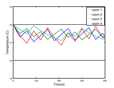
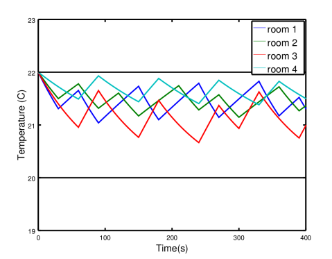
Figure 5: Simulation of the four-room case study with our synthesis method (left) and with the synthesis method of [11] (right).

5.2 DC-DC converter

This linear example is taken from [4] and has already been treated with the state-space bisection method in a linear framework in [14].

The system is a boost DC-DC converter with one switching cell. There are two switching modes depending on the position of the switching cell. The dynamics is given by the equation $\dot{x}(t)=A_{\_}{\sigma(t)}x(t)+B_{\_}{\sigma(t)}$ with $\sigma(t)\in U=\{1,2\}$. The two modes are given by the matrices:

$$A_{\_}1=\left(\begin{matrix}-\frac{r_{\_}l}{x_{\_}l}&0\\ 0&-\frac{1}{x_{\_}c}\frac{1}{r_{\_}0+r_{\_}c}\end{matrix}\right)\quad B_{\_}1=\left(\begin{matrix}\frac{v_{\_}s}{x_{\_}l}\\ 0\end{matrix}\right)$$

$$A_{\_}2=\left(\begin{matrix}-\frac{1}{x_{\_}l}(r_{\_}l+\frac{r_{\_}0.r_{\_}c}{r_{\_}0+r_{\_}c})&-\frac{1}{x_{\_}l}\frac{r_{\_}0}{r_{\_}0+r_{\_}c}\\ \frac{1}{x_{\_}c}\frac{r_{\_}0}{r_{\_}0+r_{\_}c}&-\frac{1}{x_{\_}c}\frac{r_{\_}0}{r_{\_}0+r_{\_}c}\end{matrix}\right)\quad B_{\_}2=\left(\begin{matrix}\frac{v_{\_}s}{x_{\_}l}\\ 0\end{matrix}\right)$$

with $x_{\_}c=70$, $x_{\_}l=3$, $r_{\_}c=0.005$, $r_{\_}l=0.05$, $r_{\_}0=1$, $v_{\_}s=1$. The sampling period is $\tau=0.5$. The parameters are exact and there is no perturbation. We want the state to return infinitely often to the region $R$, set here to $[1.55,2.15]\times[1.0,1.4]$, while never going out of the safety set $S=[1.54,2.16]\times[0.99,1.41]$. On this example, the Euler-based method fails while DynIBEX succeeds rapidly.

	Euler	DynIBEX
$R$	$[1.55,2.15]\times[1.0,1.4]$
$S$	$[1.54,2.16]\times[0.99,1.41]$
$\tau$	0.5
Complete control	No	Yes
$\lambda_{\_}1$	$-0.014215$
$\lambda_{\_}2$	$0.142474$
$C_{\_}{1}$	$6.7126\times 10^{-5}$
$C_{\_}{2}$	$2.6229\times 10^{-2}$
Number of balls/tiles	x	48
Pattern length	x	6
CPU time	x	< 1 second

Table 2: Numerical results for the DC-DC converter example.

5.3 Polynomial example

We consider the polynomial system taken from [20]:

$$\left[\begin{matrix}\dot{x}_{\_}1\\ \dot{x}_{\_}2\end{matrix}\right]=\left[\begin{matrix}-x_{\_}2-1.5x_{\_}1-0.5x_{\_}1^{3}+u_{\_}1\\ x_{\_}1+u_{\_}2\end{matrix}\right].$$ (6)

The control inputs are given by $u=(u_{\_}1,u_{\_}2)=K_{\_}{\sigma(t)}(x_{\_}1,x_{\_}2)$, $\sigma(t)\in U=\{1,2,3,4\}$, which correspond to four different state feedback controllers $K_{\_}1(x)=(0,-x_{\_}2^{2}+2)$, $K_{\_}2(x)=(0,-x_{\_}2)$, $K_{\_}3(x)=(2,10)$, $K_{\_}4(x)=(-1.5,10)$. We thus have four switching modes. The disturbances are not taken into account. The objective is to visit infinitely often two zones $R_{\_}1$ and $R_{\_}2$, without going out of a safety zone $S$.

	Euler	DynIBEX
$R_{\_}1$	$[-1,0.65]\times[0.75,1.75]$
$R_{\_}2$	$[-0.5,0.5]\times[-0.75,0.0]$
$S$	$[-2.0,2.0]\times[-1.5,3.0]$
$\tau$	0.15
Time subsampling	$\tau/20$
Complete control	Yes	Yes
$\lambda_{\_}1$	$-1.5$
$\lambda_{\_}2$	$-1.0$
$\lambda_{\_}3$	$-1.1992\times 10^{-8}$
$\lambda_{\_}4$	$-5.7336\times 10^{-6}$
$C_{\_}{1}$	641.37
$C_{\_}{2}$	138.49
$C_{\_}{3}$	204.50
$C_{\_}{4}$	198.64
Number of balls/tiles	16 & 16	1 & 1
Pattern length	8	7
CPU time	29 & 4203 seconds	<0.1 & 329 seconds

Table 3: Numerical results for the polynomial example example.

For Euler and DynIBEX, the table indicates two CPU times corresponding to the reachability from $R_{\_}1$ to $R_{\_}2$ and vice versa. On this example, the Euler-based method is much slower than DynIBEX.

5.4 Two-tank system

The two-tank system is a linear example taken from [17]. The system consists of two tanks and two valves. The first valve adds to the inflow of tank 1 and the second valve is a drain valve for tank 2. There is also a constant outflow from tank 2 caused by a pump. The system is linearized at a desired operating point. The objective is to keep the water level in both tanks within limits using a discrete open/close switching strategy for the valves. Let the water level of tanks 1 and 2 be given by $x_{\_}1$ and $x_{\_}2$ respectively. The behavior of $x_{\_}1$ is given by $\dot{x}_{\_}1=-x_{\_}1-2$ when the tank 1 valve is closed, and $\dot{x}_{\_}1=-x_{\_}1+3$ when it is open. Likewise, $x_{\_}2$ is driven by $\dot{x}_{\_}2=x_{\_}1$ when the tank 2 valve is closed and $\dot{x}_{\_}2=x_{\_}1-x_{\_}2-5$ when it is open. On this example, the Euler-based method works better than DynIBEX in terms of CPU time.

	Euler	DynIBEX
$R$	$[-1.5,2.5]\times[-0.5,1.5]$
$S$	$[-3,3]\times[-3,3]$
$\tau$	0.2
Time subsampling	$\tau/10$
Complete control	Yes	Yes
$\lambda_{\_}1$	0.20711
$\lambda_{\_}2$	-0.50000
$\lambda_{\_}3$	0.20711
$\lambda_{\_}4$	-0.50000
$C_{\_}{1}$	11.662
$C_{\_}{2}$	28.917
$C_{\_}{3}$	13.416
$C_{\_}{4}$	32.804
Number of balls/tiles	64	10
Pattern length	6	6
CPU time	58 seconds	246 seconds

Table 4: Numerical results for the two-tank example.

5.5 Helicopter

The helicopter is a linear example taken from [12]. The problem is to control a quadrotor helicopter toward a particular position on top of a stationary ground vehicle, while satisfying constraints on the relative velocity. Let $g$ be the gravitational constant, $x$ (reps. $y$) the position according to $x$-axis (resp. $y$-axis), $\dot{x}$ (resp. $\dot{y}$) the velocity according to $x$-axis (resp. $y$-axis), $\phi$ the pitch command and $\psi$ the roll command. The possible commands for the pitch and the roll are the following: $\phi,\psi\in\{-10,0,10\}$. Since each mode corresponds to a pair $(\phi,\psi)$, there are nine switched modes. The dynamics of the system is given by the equation:

$$\dot{X}=\begin{pmatrix}0&1&0&0\\ 0&0&0&0\\ 0&0&0&1\\ 0&0&0&0\end{pmatrix}X+\begin{pmatrix}0\\ g\sin(-\phi)\\ 0\\ g\sin(\psi)\end{pmatrix}$$

where $X=(x\ \dot{x}\ y\ \dot{y})^{\top}$. Since the variables $x$ and $y$ are decoupled in the equations and follow the same equations (up to the sign of the command), it suffices to study the control for $x$ (the control for $y$ is the opposite). On this example again, the Euler-based method works better than DynIBEX in terms of CPU time.

	Euler	DynIBEX
$R$	$[-0.3,0.3]\times[-0.5,0.5]$
$S$	$[-0.4,0.4]\times[-0.7,0.7]$
$\tau$	0.1
Time subsampling	$\tau/10$
Complete control	Yes	Yes
$\lambda_{\_}1$	0.5
$\lambda_{\_}2$	0.5
$\lambda_{\_}3$	0.5
$C_{\_}{1}$	1.77535
$C_{\_}{2}$	0.5
$C_{\_}{3}$	1.77535
Number of balls/tiles	256	35
Pattern length	7	7
CPU time	539 seconds	1412 seconds

Table 5: Numerical results for the helicopter motion example.

5.6 Analysis and comparison of results

Our method presents the advantage over the work of [11] that no numerical integration is required for the control synthesis. The computations just require the evaluation of given functions $f_{\_}j$ and (global error) functions $\delta_{\_}j$ at sampling times. The synthesis is thus a priori cheap compared to the use of numerical integration schemes (and even compared to exact integration for linear systems). However, most of the computation time is actually taken by the search for an appropriate radius $\delta$ of the balls $B_{\_}i$ ($1\leq i\leq m$) that cover $R$, and the search for appropriate patterns $\pi_{\_}i$ that make the trajectories issued from $B_{\_}i$ return to $R$.

We observe on the examples that the resulting control strategies synthesized by our method are quite different from those obtained by the Runge-Kutta method of [11] (which uses in particular rectangular tiles instead of balls). This may explain why the experimental results are here contrasted: Euler’s method works better on 3 examples and worse on the 2 others. Besides the Euler method fails on one example (DC-DC converter) while DynIBEX succeeds on all of them. Note however that our Euler-based implementation is made of a few hundreds lines of interpreted code Octave while DynIBEX is made of around five thousands of compiled code C++.

6 Final Remarks

We have given a new Euler-based method for controlling sampled switched systems, and compared it with the Runge-Kutta method of [11]. The method is remarkably simple and gives already promising results. In future work, we plan to explore the use of the backward Euler method instead of the forward Euler method used here (cf: [5]). We plan also to give general sufficient conditions ensuring the convexity of the error function $\delta_{\_}j(\cdot)$; this would allow us to get rid of the convexity tests that we perform so far numerically for each pattern.

Acknowledgement. We are grateful to Antoine Girard, Jonathan Vacher, Julien Alexandre dit Sandretto and Alexandre Chapoutot for numerous helpful discussions. This work has been partially supported by Federative Institute Farman (ENS Paris-Saclay and CNRS FR3311).

References

- [1]
- [2] M. Abbaszadeh & H.J. Marquez (2010): Nonlinear observer design for one-sided Lipschitz systems. In: Proceedings of the American Control Conference (ACC), IEEE, pp. 799–806, 10.1109/ACC.2010.5530715.
- [3] Matthias Althoff (2013): Reachability Analysis of Nonlinear Systems Using Conservative Polynomialization and Non-convex Sets. In: Proceedings of the 16th International Conference on Hybrid Systems: Computation and Control, HSCC ’13, ACM, New York, NY, USA, pp. 173–182, 10.1145/2461328.2461358.
- [4] A Giovanni Beccuti, Georgios Papafotiou & Manfred Morari (2005): Optimal control of the boost dc-dc converter. In: Decision and Control, 2005 and 2005 European Control Conference. CDC-ECC’05. 44th IEEE Conference on, IEEE, pp. 4457–4462, 10.1109/CDC.2005.1582864.
- [5] W.-J. Beyn & J. Rieger (1998): The implicit Euler scheme for one-sided Lipschitz differential inclusions. Discr. and Cont. Dynamical Systems B(14), pp. 409–428, 10.3934/dcdsb.2010.14.409.
- [6] Olivier Bouissou, Alexandre Chapoutot & Adel Djoudi (2013): Enclosing Temporal Evolution of Dynamical Systems Using Numerical Methods. In: NASA Formal Methods, LNCS 7871, Springer, pp. 108–123, 10.1007/978-3-642-38088-48.
- [7] Olivier Bouissou, Samuel Mimram & Alexandre Chapoutot (2012): HySon: Set-Based Simulation of Hybrid Systems. In: Rapid System Prototyping, IEEE, 10.1109/RSP.2012.6380694.
- [8] Xiushan Cai, Zhenyun Wang & Leipo Liu (2015): Control Design for One-side Lipschitz Nonlinear Differential Inclusion Systems with Time-delay. Neurocomput. 165(C), pp. 182–189, 10.1016/j.neucom.2015.03.008.
- [9] Xin Chen, Erika Abraham & Sriram Sankaranarayanan (2012): Taylor Model Flowpipe Construction for Non-linear Hybrid Systems. In: IEEE 33rd Real-Time Systems Symposium, IEEE Computer Society, pp. 183–192, 10.1109/RTSS.2012.70.
- [10] Xin Chen, Erika Ábrahám & Sriram Sankaranarayanan (2013): Flow*: An analyzer for non-linear hybrid systems. In: Computer Aided Verification, Springer, pp. 258–263, 10.1007/978-3-642-39799-818.
- [11] A. Le Coënt, J. Alexandre dit Sandretto, A. Chapoutot & L. Fribourg (2016): Control of nonlinear switched systems based on validated simulation. In: 2016 International Workshop on Symbolic and Numerical Methods for Reachability Analysis (SNR), pp. 1–6, 10.1109/SNR.2016.7479377.
- [12] Jerry Ding, Eugene Li, Haomiao Huang & Claire J Tomlin (2011): Reachability-based synthesis of feedback policies for motion planning under bounded disturbances. In: Robotics and Automation (ICRA), 2011 IEEE International Conference on, IEEE, pp. 2160–2165, 10.1109/ICRA.2011.5980268.
- [13] Tzanko Donchev & Elza Farkhi (1998): Stability and Euler Approximation of One-sided Lipschitz Differential Inclusions. SIAM J. Control Optim. 36(2), pp. 780–796, 10.1137/S0363012995293694.
- [14] Laurent Fribourg, Ulrich Kühne & Romain Soulat (2014): Finite controlled invariants for sampled switched systems. Formal Methods in System Design 45(3), pp. 303–329, 10.1007/s10703-014-0211-2.
- [15] Antoine Girard (2005): Reachability of uncertain linear systems using zonotopes. In: Hybrid Systems: Computation and Control, Springer, pp. 291–305, 10.1007/978-3-540-31954-219.
- [16] Antoine Girard, Giordano Pola & Paulo Tabuada (2010): Approximately bisimilar symbolic models for incrementally stable switched systems. IEEE Transactions on Automatic Control 55(1), pp. 116–126, 10.1007/978-3-540-78929-115.
- [17] Ian A Hiskens (2001): Stability of limit cycles in hybrid systems. In: System Sciences, 2001. Proceedings of the 34th Annual Hawaii International Conference on, IEEE, 10.1109/HICSS.2001.926280.
- [18] Fabian Immler (2015): Verified reachability analysis of continuous systems. In: Tools and Algorithms for the Construction and Analysis of Systems, Springer, pp. 37–51, 10.1007/978-3-662-46681-03.
- [19] Frank Lempio (1995): Set-Valued Interpolation, Differential Inclusions, and Sensitivity in Optimization. In: Recent Developments in Well-Posed Variational Problems, Kluwer Academic Publishers, pp. 137–169, 10.1007/978-94-015-8472-26.
- [20] Jun Liu, Necmiye Ozay, Ufuk Topcu & Richard M Murray (2013): Synthesis of reactive switching protocols from temporal logic specifications. Automatic Control, IEEE Transactions on 58(7), pp. 1771–1785, 10.1109/TAC.2013.2246095.
- [21] Kyoko Makino & Martin Berz (2009): Rigorous Integration of Flows and ODEs Using Taylor Models. In: Proceedings of the 2009 Conference on Symbolic Numeric Computation, SNC ’09, ACM, New York, USA, pp. 79–84, 10.1145/1577190.1577206.
- [22] Pierre-Jean Meyer (2015): Invariance and symbolic control of cooperative systems for temperature regulation in intelligent buildings. Thèse, Université Grenoble Alpes.
- [23] Ramon Moore (1966): Interval Analysis. Prentice Hall.
- [24] Nedialko S. Nedialkov, K. Jackson & Georges Corliss (1999): Validated solutions of initial value problems for ordinary differential equations. Appl. Math. and Comp. 105(1), pp. 21 – 68, 10.1016/S0096-3003(98)10083-8.
- [25] J. Alexandre dit Sandretto & A. Chapoutot (2015): Validated Solution of Initial Value Problem for Ordinary Differential Equations based on Explicit and Implicit Runge-Kutta Schemes. Research Report, ENSTA ParisTech.
- [26] Julien Alexandre dit Sandretto & Alexandre Chapoutot (2015): DynIbex library. Http://perso.ensta-paristech.fr/ chapoutot/dynibex/.
- [27] Julien Alexandre dit Sandretto & Alexandre Chapoutot (2016): Validated explicit and implicit runge-kutta methods. Reliable Computing 22, pp. 79–103.
- [28] J. Stolfi & L. H. de Figueiredo (1997): Self-Validated Numerical Methods and Applications. Brazilian Mathematics Colloquium monographs, IMPA/CNPq.