Universal black hole stability in four dimensions

Abstract

We show that four-dimensional black holes become stable below certain mass when the Einstein-Hilbert action is supplemented with higher-curvature terms. We prove this to be the case for an infinite family of ghost-free theories involving terms of arbitrarily high order in curvature. The new black holes, which are non-hairy generalizations of Schwarzschild’s solution, present a universal thermodynamic behavior for general values of the higher-order couplings. In particular, small black holes have infinite lifetimes. When the evaporation process makes the semiclassical approximation break down (something that occurs after a time which is usually infinite for all practical purposes), the resulting object retains a huge entropy, in stark contrast with Schwarzschild’s case.

I Introduction

As proven by Hawking Hawking (1975), a black hole with surface gravity $\kappa$ emits thermal radiation with a temperature $T_{\scriptscriptstyle\rm H}=\kappa/(2\pi)$. In the prototypical case of a Schwarzschild black hole Schwarzschild (1916) of initial mass $M_{0}$, the temperature increases as the black hole radiates, as a consequence of its negative specific heat. After a finite time of order $\sim M_{0}^{3}/M_{\rm\scriptscriptstyle P}^{4}$, where $M_{\rm\scriptscriptstyle P}$ is the Planck mass, the black hole evaporates down to an order-$M_{\rm\scriptscriptstyle P}$ object of order-one entropy. This suggests a violent ending for the evaporation process, and gives rise to the information paradox (see Harlow (2016); Chen et al. (2015) for recent reviews): a pure state collapsed to form a black hole would evolve into thermal radiation, in tension with the unitary evolution expected from quantum mechanics — see Myers (1997), though. Before the evaporation process has come to an end, one could hope that the black hole acts as an information reservoir (so that, e.g., pure states are still pure when one does not trace out over the interior degrees of freedom). This is however very difficult to sustain, given the extremely low entropy of the Planck-mass object towards which the black hole evolves — see also the discussion at the end of Section VI.

These considerations rely, in particular, on the somewhat unusual thermodynamic properties of the Schwarzschild black hole, which is expected to be the correct description of the exterior gravitational field of any static and spherically symmetric matter configuration for small enough curvatures. On the other hand, the effective gravitational action is expected to contain an infinite series of higher-derivative corrections modifying the usual Einstein-Hilbert term — see e.g., Nepomechie (1985); Gross and Witten (1986); Gross and Sloan (1987); ’t Hooft and Veltman (1974); Deser and van Nieuwenhuizen (1974). One is then naturally led to wonder how these terms modify Schwarzschild’s solution in higher-curvature situations and how such modifications might affect its thermodynamic behavior, as well as the evaporation process — see e.g., Myers and Simon (1988, 1989); Callan et al. (1989) for progress in this direction (mostly in higher-dimensions).

Unfortunately, constructing non-trivial extensions of the four-dimensional Schwarzschild black hole in higher-derivative gravities is a far from trivial task — see e.g., Lu et al. (2015a, b). For example, as opposed to the $D\geq 5$ cases, all the higher-order Lovelock invariants Lovelock (1970, 1971) — which due to their special properties do allow for such simple extensions, e.g., Boulware and Deser (1985); Wheeler (1986); Myers and Simon (1988); Cai (2002); Dehghani and Pourhasan (2009); de Boer et al. (2010a) — are trivial in $D=4$.

Recently, the construction of Einsteinian cubic gravity Bueno and Cano (2016a), has triggered the construction of new four- (and higher-)dimensional generalizations of the Schwarzschild black hole Hennigar and Mann (2016); Bueno and Cano (2016b); Hennigar et al. (2017); Bueno and Cano (2017); Ahmed et al. (2017). These solutions share the property of being fully determined by a single metric function, i.e., they can be written in Schwarzschild-like coordinates as

$$ds_{f}^{2}=-f(r)dt^{2}+f(r)^{-1}dr^{2}+r^{2}d\Omega_{(2)}^{2}\,,$$ (1)

a characteristic which turns out to be related to the absence of ghosts in the linearized spectrum of the theory Myers and Robinson (2010); Bueno and Cano (2017). Besides, the new black holes are non-hairy and fully characterized by their mass $M$, they describe the exterior field of spherical mass distributions Bueno and Cano (2017), and reduce to Schwarzschild’s solution when the corresponding higher-derivative couplings are set to zero.

In this paper, we will argue that these black holes are particular cases of an infinite family of four-dimensional solutions to a gravity theory involving terms of arbitrarily high order in curvature. As opposed to Schwarzschild’s, the specific heat of the new black holes becomes positive below certain mass, which completely changes the evaporation process. In particular, the new small black holes have infinite lifetimes. Besides, following the evaporation process till the point in which the semiclassical approximation breaks down, one finds that a naturally enormous time is required and that the resulting object has a huge entropy, in flagrant contrast with the Schwarzschild black hole case — see Table 1 below for a summary. In the small mass regime, the new (asymptotically flat) black holes satisfy the Smarr-type relation: $M=\frac{2}{3}TS$, which, intriguingly, coincides with the result corresponding to a three-dimensional CFT at finite temperature. We argue that the above properties are universal for general values of the higher-order couplings.

II Higher-order corrections

The four-dimensional theories studied in Bueno and Cano (2016a); Hennigar and Mann (2016); Bueno and Cano (2016b); Hennigar et al. (2017); Bueno and Cano (2017) and Ahmed et al. (2017) are cubic and quartic representatives of an infinite family of higher-order gravities admitting simple extensions of the Schwarzschild solution whose thermodynamic properties can be easily accessed. The Lagrangian of this family can be written as

$$\mathcal{L}=\frac{1}{16\pi G}\left[R+\sum_{n=3}^{\infty}\frac{\lambda_{n}}{M_{c}^{2(n-1)}}\mathcal{R}_{(n)}\right]\,,$$ (2)

where $G=1/M_{\rm\scriptscriptstyle P}^{2}$ is the Newton constant, $M_{c}$ is some new energy scale, $\lambda_{n}$ are dimensionless couplings and $n$ is the order in curvature of each invariant $\mathcal{R}_{(n)}$, which will be formed by contractions of the metric and the Riemann tensor (but not its covariant derivatives).

The $\mathcal{R}_{(n)}$ are constructed using the following criterion. Let $L_{f}$ be the effective Lagrangian resulting from the evaluation of $\sqrt{|g|}\mathcal{L}$ on the ansatz (1), i.e., $L_{f}\equiv\sqrt{|g|}\mathcal{L}\rvert_{g^{ab}=g_{f}^{ab}}.$ Then, we select the $\mathcal{R}_{(n)}$ in a way such that the Euler-Lagrange equation of $f(r)$ associated to $L_{f}$ vanishes identically, i.e., for all $f(r)$. As shown in Bueno and Cano (2017), any theory of the form (2) fulfilling this requirement, satisfies the following properties: 1) it allows for solutions of the form (1), where $f(r)$ is determined by a second-order differential equation; 2) these solutions describe the exterior gravitational field of a static and spherically symmetric mass distribution; 3) the solutions are fully characterized by the total mass $M$; 4) the linearized equations on the vacuum are the same as Einstein gravity’s (up to an overall constant), which in particular implies that the theory spectrum is free of ghost modes — see appendix D.

Interestingly, for a given order $n$, there is a single possible way of modifying the $(n-1)$-order solution. In other words, once we find a particular density $\mathcal{R}_{n}^{A}$ contributing non-trivially to the equation determining $f(r)$, there does not exist a different density $\mathcal{R}_{n}^{B}$ which contributes in a different way to the same equation. There is however an important level of degeneracy on the $\mathcal{R}_{n}$ (growing with $n$), namely, there are several independent densities which give rise to the same equation (connected through the addition of densities which do not modify the equations of motion when evaluated on a general static and spherically symmetric ansatz). This is the case, for example, of the Einsteinian cubic gravity Bueno and Cano (2016a) and Generalized quasitopological gravity Hennigar et al. (2017) densities in the cubic case.

Our interest in this paper lies on the thermodynamic properties of the solutions, which are not affected by the particular representative $\mathcal{R}_{(n)}$ chosen at a given order. Information about the explicit form of the $\mathcal{R}_{(n)}$ for general values of $n$ is provided in appendix A. For the sake of completeness, let us at least mention that particularly nice invariants for $n=3$ and $n=4$ are given, respectively, by: $\mathcal{R}_{(3)}=-\frac{1}{6}(12\tensor{R}{{}_{a}^{b}{}_{c}^{d}}\tensor{R}{{}_{b}^{e}{}_{d}^{f}}\tensor{R}{{}_{e}^{a}{}_{f}^{c}}+R_{ab}^{cd}R_{cd}^{ef}R_{ef}^{ab}-12\tensor{R}{{}_{abcd}}\tensor{R}{{}^{ac}}\tensor{R}{{}^{bd}}+8R^{b}_{a}R_{b}^{c}R_{c}^{a})$ and $\mathcal{R}_{(4)}=+\frac{2}{3}(10R^{abcd}R_{a\ c}^{\ e\ f}R_{e\ b}^{\ g\ h}R_{fgdh}+4R^{ab}R^{cdef}R_{c\ ea}^{\ h}R_{dhfb}-14R^{abcd}R_{ab}^{\ \ ef}R_{c\ e}^{\ g\ h}R_{dgfh}-5R^{abcd}R_{a\ c}^{\ e\ f}R_{e\ f}^{\ g\ h}R_{bgdh}).$ These densities belong to the Einsteinian class Bueno and Cano (2016a); Bueno et al. (2017), i.e., when considered in (2), the corresponding theories share the linearized spectrum of Einstein gravity not only in $D=4$, but also when considered in arbitrary higher dimensions.

III Black holes

When evaluated in the ansatz (1), the field equations of (2) reduce to the following (single) second-order differential equation for $f(r)$

$$2GM-(1-f)r=-\sum_{n=3}^{\infty}\frac{\lambda_{n}}{M_{c}^{2(n-1)}}\left(\frac{f^{\prime}}{r}\right)^{n-3}\left[\frac{f^{\prime 3}}{n}+\frac{(n-3)f+2}{(n-1)r}f^{\prime 2}-\frac{2}{r^{2}}f(f-1)f^{\prime}-\frac{1}{r}ff^{\prime\prime}\left(f^{\prime}r-2(f-1)\right)\right]\,,$$ (3)

where $M$ stands for the ADM mass of the solution Arnowitt et al. (1960a, b, 1961). For $n=3$ and $n=4$, the above equation agrees with the ones found for Einsteinian cubic gravity Bueno and Cano (2016b); Hennigar and Mann (2016) and the quartic version Ahmed et al. (2017) of Generalized quasitopological gravity Hennigar et al. (2017). The general version of this equation for arbitrary values of the cosmological constant and general horizon geometries can be found in appendix C.

Observe that all terms in the sum contribute to the equation in a very similar fashion, which will ultimately be responsible for the universal thermodynamic properties of the solutions. In order for (1) to represent a black hole solution, we need to impose asymptotic flatness, as well as the existence of a regular horizon for some $r=r_{h}>0$.

In the asymptotic region, the Einstein gravity contribution dominates $f(r)$, and the higher-order corrections can be assumed to be small. These considerations lead to the following asymptotic expansion:

$$f(r)=1-\frac{2GM}{r}\left[1+\frac{18\lambda_{3}(GM/r)^{5}}{(GMM_{c})^{4}}+\cdots\right]+f_{\rm\scriptscriptstyle h}(r)\,,$$ (4)

where the dots stand for subleading contributions on $GM/r$ (including terms proportional to the higher-order couplings), and

$$f_{\rm\scriptscriptstyle h}(r)\sim A\exp\left(\frac{2r^{5/2}}{5G\sqrt{6\lambda_{3}GM}}\right)+B\exp\left(\frac{-2r^{5/2}}{5G\sqrt{6\lambda_{3}GM}}\right)\,.$$ (5)

Hence, in order to get an asymptotically flat solution, we must set $A=0$, which is equivalent to fixing one of the two integration constants in (3). Observe that in order for this conclusion to hold, we must demand the lowest-order non-vanishing $\lambda_{n}$ to be positive (we chose this to be $\lambda_{3}$ in (4)). Otherwise, we would obtain non-decaying oscillating solutions which would not be asymptotically flat in general. The second term in (5) can be neglected for practical purposes, as the decaying exponential is extremely subleading in (4).

Imposing the existence of a regular event horizon fixes the remaining integration constant. In order to see this, it is convenient to perform a Taylor expansion at the horizon,

$$f(r)=4\pi(r-r_{h})T+\sum_{n=2}^{\infty}a_{n}(r-r_{h})^{n},$$ (6)

where $T$ is the black hole temperature and $a_{n}=f^{(n)}(r_{h})/n!$. Solving (3) for the first two orders in $(r-r_{h})$ gives rise to the following relations:

$$2GM=r_{h}-\sum_{n=3}^{\infty}\frac{\lambda_{n}(4\pi T)^{n-1}}{M_{c}^{2n-2}r_{h}^{n-2}}\frac{(2n+(n-1)4\pi Tr_{h})}{n(n-1)}\,,$$ (7)

$$1= 4\pi Tr_{h}+\sum_{n=3}^{\infty}\frac{\lambda_{n}(4\pi T)^{n-1}}{M_{c}^{2n-2}r_{h}^{n-1}}\frac{(2n+(n-3)4\pi Tr_{h})}{n(n-1)}.$$ (8)

These equations fix $r_{h}$ and $T$ in terms of the black hole mass $M$. Note that these relations are exact, as they are necessary conditions for having a smooth near-horizon geometry. Depending on the values of the $\lambda_{n}$ and the mass, these equations can have one, several, or even no solutions at all. If there are several solutions, it means that various possible black holes with the same mass can exist. However, only one of the solutions will smoothly reduce to Schwarzschild in the limit $\lambda_{n}\rightarrow 0$ for all $n$. This is the one which should be regarded as physical. We will be mostly interested in the case in which there is a unique solution for any value of $M$, in whose case we can write $T(M)$ and $r_{h}(M)$ without ambiguity. This happens, for example, if $\lambda_{n}\geq 0$ for all $n$, which, at the same time ensures the solution to be well-behaved asymptotically.

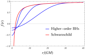
Figure 1: Metric function $f(r)$ for Schwarzschild’s solution (red) and for the new higher-order black holes (blue), with $\lambda_{3}=\lambda_{4}=\lambda_{5}=\lambda_{6}=1$, $\lambda_{n>6}=0$ and $GMM_{c}=0.5\,,0.2\,,0.1$ respectively, (from left to right).

Once $T(M)$ and $r_{h}(M)$ have been determined, the $(r-r_{h})^{2}$-order equation fixes $a_{3}$ as a function of $a_{2}=f^{\prime\prime}(r_{h})/2$, the $(r-r_{h})^{3}$ one fixes $a_{4}$ as a function of $a_{3}$ and $a_{2}$, and so on. In this process the only undetermined parameter is $a_{2}$, which means that the solution will be fully determined once we choose a value for it. Therefore, the family of solutions with a regular horizon is characterized by a single parameter, which must be carefully chosen so that the solution is asymptotically flat. In all cases studied, a numerical analysis shows that there is a unique value of $a_{2}$ for which asymptotic flatness is achieved. This means that there exists a unique asymptotically flat black hole, fully characterized by its mass $M$, which reduces to Schwarzschild’s solution when the higher-order couplings are set to zero. The results presented in Bueno and Cano (2017) imply that, just like for Schwarzschild in the Einstein gravity case, this will also represent the exterior field of a generic spherically symmetric matter distribution.

In appendix B, we provide a detailed discussion of the numerical construction of the solutions (which, unfortunately, do not seem accesible analitically). The resulting metric functions, $f(r)$, for a particular set of $\lambda_{n}$ and different values of $M_{c}$ are shown in Fig. 1. Changing the $\lambda_{n}$ does not modify these curves qualitatively.

IV Thermodynamics

Making use of Wald’s formula Wald (1993), it is possible to compute the entropy of the solutions, which yields

$$S=\frac{\pi r_{h}^{2}}{G}\left[1-2\sum_{n=3}^{\infty}\frac{\lambda_{n}(4\pi T)^{n-1}}{M_{c}^{2n-2}r_{h}^{n-1}}\cdot\right.$$ (9)

$$\left.\cdot\left(\frac{2}{(n-2)4\pi Tr_{h}}+\frac{1}{n-1}\right)\right]+\frac{4\pi}{GM_{c}^{2}}\sum_{n=3}^{\infty}\frac{\lambda_{n}\chi^{n-2}}{(n-2)}\,,$$

where $\chi$ is defined as

$$\sum_{n=3}^{\infty}\frac{2\lambda_{n}\chi^{n-1}}{(n-1)}\equiv 1\,.$$ (10)

Using (9), we verify that the first law, $dM=TdS$, is satisfied. The last term in (9) is a constant that ensures that $S\rightarrow 0$ as $M\rightarrow 0$, something that can always be done by adding a particular total derivative term to the original action (2) (e.g., an explicit Gauss-Bonnet contribution).

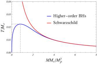
Figure 2: Black hole temperature as a function of the mass for Schwarzschild’s solution (red) and for the higher-order black holes with $\lambda_{3}=\lambda_{4}=\lambda_{5}=\lambda_{6}=1$, $\lambda_{n>6}=0$ (note that the blue line is valid for any $M_{c}$). The higher-order black holes become stable below $M_{\rm\scriptscriptstyle max}\sim M_{\rm\scriptscriptstyle P}^{2}/M_{c}$. The shape of this curve is qualitatively the same for any other choice of couplings (except $\lambda_{n}=0$ for all $n$).

As opposed to the case of the Schwarzschild black hole, the temperature of the new solutions reaches a maximum for certain value of the mass, $M_{\rm\scriptscriptstyle max}\sim M_{\rm\scriptscriptstyle P}^{2}/M_{c}$. As shown in Fig. 2, black holes with large enough masses behave like Schwarzschild’s. However, when $M<M_{\rm\scriptscriptstyle max}$, the specific heat of the solutions becomes positive, which implies that small black holes behave as ordinary thermodynamic systems. Hence, for instance, they become colder as they radiate, and they tend to reach equilibrium in the presence of a thermal environment. This behavior takes place as soon as one of the higher-order couplings is non-zero. Remarkably, turning on additional couplings does not modify this behavior qualitatively. All the possible black holes corresponding to the infitely many possible choices of $\lambda_{n}$ $(\geq 0)$ belong to the same universality class, the only exception being Schwarzshchild’s black hole.

When the mass is much smaller than the corresponding maximum value, $M\ll M_{\rm\scriptscriptstyle max}$, the expressions for $r_{h}(M)$, $S(M)$ and $T(M)$ are approximately given by

$$r_{h} =\left[\frac{M}{\zeta\chi^{3}M_{c}^{2}M_{\rm\scriptscriptstyle P}^{2}}\right]^{1/3}\,,\,\,S=6\pi\left[\frac{\zeta^{1/2}MM_{\rm\scriptscriptstyle P}}{M_{c}^{2}}\right]^{2/3}\,,$$ (11)

$$T =\frac{1}{4\pi}\left[\frac{MM_{c}^{4}}{\zeta M_{\rm\scriptscriptstyle P}^{2}}\right]^{1/3}\,,\text{ where}\quad\zeta\equiv\sum_{n=3}^{\infty}\frac{\lambda_{n}\chi^{n-3}}{n}\,.$$ (12)

In this regime, the solutions satisfy the Smarr relation

$$M=\frac{2}{3}TS\,,$$ (13)

which turns out to coincide with the result corresponding to a three-dimensional CFT at finite temperature (if we identify $M$ with the CFT energy density). Note that (13) is valid for arbitrary values of $\lambda_{n}$ as long as at least one of them is non-vanishing. This is a quite intriguing result. In fact, (13) coincides also with the result found for planar asymptotically Anti-de Sitter (AdS) black holes, as expected from the AdS/CFT correspondence Maldacena (1999); Witten (1998); Gubser et al. (1998). In contrast, (13) holds here for the spherically symmetric and asymptotically flat black holes of the theory (2) in the small mass limit. Note that (13) differs from Schwarzschild’s analogous relation, which reads $M=2TS$ instead (observe that such relation is also valid for general $\lambda_{n}$ when $M\gg M_{\rm\scriptscriptstyle max}$).

V Black hole evaporation

	Semiclassical approximation breakdown mass	Time till $M\sim M_{\rm\scriptscriptstyle min}$	Entropy when $M\sim M_{\rm\scriptscriptstyle min}$
Schwarzschild	$M_{\rm\scriptscriptstyle min}\sim M_{\rm\scriptscriptstyle P}$	$\Delta t\sim M_{0}^{3}/M_{\scriptscriptstyle\rm P}^{4}$	$S\sim 1$
Higher-order BHs	$M_{\rm\scriptscriptstyle min}\sim\sqrt{M_{\scriptscriptstyle\rm P}M_{c}}$	$\Delta t\sim M_{\rm\scriptscriptstyle P}^{7/2}/M_{c}^{9/2}$	$S\sim M_{\rm\scriptscriptstyle P}/M_{c}$

Table 1: We compare the result of the evaporation process for a Schwarzschild black hole to the one for the new higher-order solutions at the scale for which the semiclassical approximation stops making sense. When the minimum mass is reached, the Schwarzschild black hole has turned into a Planck-mass object of order-one entropy. For the new black holes, the entropy of the resulting object is huge instead.

Let us now explore how the evaporation process of black holes gets affected by the special thermodynamic behavior of the new solutions in the small mass regime. The rate of mass-loss of a black hole in the vacuum can be computed using the Stefan-Boltzmann law,

$$\frac{dM(t)}{dt}=-4\pi r_{h}^{2}\sigma\cdot T^{4}\,,$$ (14)

where $\sigma=\pi^{2}/60$. Using (11), we can easily integrate this expression for $M\ll M_{\rm\scriptscriptstyle max}$. The result is

$$M(t)=\frac{M_{0}}{1+t/t_{1/2}}\,,\quad\text{where}\quad t_{1/2}=\frac{3840\pi\chi^{2}\zeta^{2}M_{\rm\scriptscriptstyle P}^{4}}{M_{0}M_{c}^{4}}\,,$$ (15)

is the half-life of the black hole. Then, we observe that an infinite time is required for the black holes to evaporate completely. Note also that the half-life is huge as long as $M_{c}\ll M_{\scriptscriptstyle\rm P}$. This condition can be easily made compatible with the requirement that the physics of macroscopic black holes does not get affected by the new couplings, which can be expressed as: $M_{c}\gg(GM_{\odot})^{-1}\sim 10^{-9}$ eV.

The regime of validity of the semiclassical description is characterized by the fact that the horizon radius is much greater than the corresponding Compton wavelength, i.e., $r_{h}\gg\lambda_{\rm\scriptscriptstyle Compton}\sim 1/M$. Similarly, the thermodynamic description is valid whenever $S\gg 1$, and breaks down as $S\sim 1$. A Schwarzschild black hole reaches the Planck mass in a time $\Delta t\sim M_{0}^{3}/M_{\rm\scriptscriptstyle P}^{4}$, after which both conditions are violated. In contrast, for the new black holes, the condition on the entropy is never violated as long as we choose $M_{c}\ll M_{\scriptscriptstyle\rm P}$. The semiclassical approximation stops making sense for a mass of order

$$M_{\rm\scriptscriptstyle min}\sim\zeta^{1/4}\chi^{3/4}\sqrt{M_{\scriptscriptstyle\rm P}M_{c}}\,.$$ (16)

Interestingly, when such a mass is reached, the entropy is still very large, namely

$$S_{\rm\scriptscriptstyle min}\sim\sqrt{\chi\zeta}\frac{M_{\rm\scriptscriptstyle P}}{M_{c}}\,.$$ (17)

Starting with a black hole of initial mass $M_{\rm\scriptscriptstyle min}\ll M_{0}\ll M_{\rm\scriptscriptstyle max}$, the minimum mass is reached in a time

$$\Delta t\sim\chi^{5/4}\zeta^{7/4}\frac{M_{\rm\scriptscriptstyle P}^{7/2}}{M_{c}^{9/2}}\,,$$ (18)

which, remarkably, does not depend on $M_{0}$ as long as $M_{0}\gg M_{\rm\scriptscriptstyle min}$. We summarize these observations in Table 1.

It is illustrative to make a quantitative comparison with the Schwarzschild case. If we choose, say, $M_{c}\sim 1$ GeV, the temperature maximum would be at $M_{\rm\scriptscriptstyle max}\sim 10^{13}$ kg, and the semiclassical approximation break down mass would be $M_{\rm\scriptscriptstyle min}\sim 10^{6}$ TeV. At that point, the entropy would be of order $S_{\rm\scriptscriptstyle min}\sim 10^{19}$. In contrast, a Schwarzschild black hole of mass $M_{0}\sim 10^{6}$ kg, would evaporate down to the Planck mass in $\Delta t\sim 1$ minute, with a final entropy $S\sim 1$. One of the new higher-order black holes with the same initial mass (or, in fact, with any mass such that $M_{\rm\scriptscriptstyle min}\ll M_{0}\ll M_{\rm\scriptscriptstyle max}$), would need $\Delta t\sim 10^{25}$ times the age of the universe to reach $M_{\rm\scriptscriptstyle min}$. Hence, in contrast to the Schwarzschild case, the lifetime of the new small black holes (understood, in this case, as the period till the semiclassical approximation breakdown) is usually huge or, rather, infinite for all practical purposes.

Let us close this section by mentioning that one could of course consider the evaporation process of black holes with $M_{0}>M_{\rm\scriptscriptstyle max}$ as well. In that case, the process would be Schwarzschild-like till the black hole reaches the point for which the remaining mass is smaller than $M_{\rm\scriptscriptstyle max}$. After that, the discussion in this section would start applying. Of course, this implies that all black holes — big or small — belonging to the new family have infinite lifetimes.

VI Conclusions

In this paper, we have presented an infinite family of four-dimensional higher-order gravities admitting non-hairy, static and spherically symmetric generalizations of the Schwarzschild black hole. The new theories, defined in (2), have the same linearized spectrum as Einstein gravity, which implies, in particular, that no ghost modes are propagated by metric perturbations on the vacuum.

The new solutions, which reduce to Schwarzschild’s when all the higher-order couplings are set to zero, present a thermodynamic behavior which notably differs from the one encountered in the Schwarzschild black hole. In particular, the specific heat of the black holes becomes positive below certain mass $M_{\rm\scriptscriptstyle max}\sim M_{\rm\scriptscriptstyle P}^{2}/M_{c}$, where $M_{c}$ is a new scale — see Fig. 2. This behavior is universal for all the possible choices of the higher-order couplings $\lambda_{n}\geq 0$ with the only exception of Schwarzschild’s solution itself.

Even though the solutions cannot be constructed analytically — see appendix B for a detailed discussion of the numerical construction —, the relevant thermodynamic magnitudes can be accessed exactly and, in particular, explicit expressions for the horizon radius, the temperature and the entropy as functions of the black hole mass $M$ can be written for small enough masses, $M\ll M_{\rm\scriptscriptstyle max}$ — see equations (11) and (12). In this regime, the black holes satisfy the Smarr relation $M=2/3\cdot TS$ for arbitrary values of the new couplings (as long as at least one of them is non-vanish) which, intriguingly, is analogous to the one found for a three-dimensional CFT at finite temperature.

The thermodynamic properties of the small higher-order black holes have dramatic consequences for the evaporation process. In particular, as opposed to the Schwarzschild case, the new black holes have infinite lifetimes, so one could speculate that they might act as eternal information reservoirs evading possible unitarity violations. During the evaporation, the black holes require a (normally huge) time $\Delta t\sim M_{\rm\scriptscriptstyle P}^{7/2}/M_{c}^{9/2}$ to reach a mass $M_{\rm\scriptscriptstyle min}\sim\sqrt{M_{\rm\scriptscriptstyle P}M_{c}}$ for which the semiclassical description breaks down. At that point, the entropy of the resulting object is still huge, $S\sim M_{\rm\scriptscriptstyle P}/M_{c}$. This is in stark contrast with the Schwarzschild black hole case, which reaches the Planck mass with an order-one entropy. One can only speculate on what would happen below $M_{\rm\scriptscriptstyle min}$. However, it is worth emphasizing that the tendency suggested by the evaporation process of the new black holes is very different from Schwarschild’s: first, if we extrapolated the semiclassical approximation beyond $M_{\rm\scriptscriptstyle min}$, the Schwarzschild black hole would disappear soon after, while the new black holes would placidly keep on living forever; and second, at the semiclassical breakdown point, the issue of being left with an extremely low entropy object gets notably softened.

At this point, it is convenient to stress that attempts to resolve the information paradox involving remnant-like objects Aharonov et al. (1987) have been usually argued to be very difficult to digest Preskill (1992); Harvey and Strominger (1993); Giddings (1995); Susskind (1995). This is, in particular, because one can consider the evaporation process of arbitrary initial black holes, which would imply that an arbitrarily large amount of information would need to be stored in the remnant, forcing such finite-energy object to have an infinite number of internal states (or, in other words, infinitely many “species” of remnants would need to exist, one for each possible initial state collapsing to a black hole). This raises the question of how an arbitrary amount of information could be carried within a Planck volume (or, more generally, the volume associated to the semiclassical breakdown scale) and naturally leads to a problematic infinite production rate of remnant pairs — see e.g., Giddings (1995). While these remain outstanding issues, our results illustrate that the evaporation process can drastically change when higher-order terms are considered in the gravitational effective action, suggesting new perspectives for the final fate of black holes or, at least, for the way they approach the regime in which the semiclassical description stops making sense.

Let us close with some possible future directions. Firstly, it would be convenient to understand how common the thermodynamic properties of the black holes presented here are among other (perhaps more general) higher-derivative corrections to the Einstein-Hilbert action. A different venue worth exploring would entail trying to find out whether some of the new higher-order invariants, $\mathcal{R}_{(n)}$, can actually arise as $\alpha^{\prime}$ corrections in concrete four-dimensional String theory effective actions. One would naively expect that, just like the $\mathcal{R}_{(n)}$, such terms should not give rise to ghosts in the linearized spectrum so, at least from this perspective, there seems to be a chance that this is the case.

It would also be interesting to study other consequences derived from the possible existence of small stable black holes in four dimensions. For example, it has been often argued that microscopic black holes could be responsible for dark matter — see e.g., Chen and Adler (2003); Easson (2003); Afshordi et al. (2003); Nozari and Mehdipour (2005); Mureika (2012). While the existence of microscopic Schwarzschild black holes is not allowed due to their rapid evaporation, the stability of the new black holes seems to make them suitable for this purpose.

Appendix A Explicit form of the higher-order invariants

At each order in curvature, there do not exist two invariants $\mathcal{R}_{(n)}^{A}$ and $\mathcal{R}_{(n)}^{B}$ giving rise to two different non-trivial contributions to the equation determining the metric function, (3), compatible with the ansatz (1). There is a unique contribution, which is nothing but the one which appears inside the sum in the rhs of (3). However, as we explained in the main text, the invariants $\mathcal{R}_{(n)}$ are uniquely defined only up to the addition of terms which do not modify the equations of motion for a general static and spherically symmetric ansatz. For example, one can always modify $\mathcal{R}_{(n)}$ by the addition of the corresponding $n$-th order Lovelock density. In fact, there exists a considerable amount of freedom when choosing the set of $\mathcal{R}_{(n)}$ invariants for which (2) admits solutions of the form (1). In the main text, we presented a particular choice of invariants for the $n=3,4$ cases. Those present the additional particularity of sharing the linearized spectrum of Einstein gravity (not only in four dimensions, but) for general $D$, while being defined in the same way in arbitrary dimensions (i.e., the relative couplings of each invariant do not depend on $D$, like in the case of Lovelock theories). The general procedure for constructing Einsteinian gravities, which was explained in Bueno and Cano (2016a); Bueno et al. (2017), could be used to determine whether it is always possible to find examples of $\mathcal{R}_{(n)}$ belonging to this class for $n\geq 5$.

A simpler approach for constructing high-order invariants consists in considering products of lower-order densities. In particular, we claim that $5$ densities suffice to construct examples of $\mathcal{R}_{(n)}$ at any order. These densities can be chosen to be

$$R\,,\quad Q_{1}\equiv R_{ab}R^{ab}\,,\quad Q_{2}\equiv R_{abcd}R^{abcd}\,,\quad C_{1}\equiv\tensor{R}{{}_{a}^{b}{}_{c}^{d}}\tensor{R}{{}_{b}^{e}{}_{d}^{f}}\tensor{R}{{}_{e}^{a}{}_{f}^{c}}\,,\quad C_{2}\equiv R_{ab}^{cd}R_{cd}^{ef}R_{ef}^{ab}\,.$$ (19)

Using the Ricci scalar, the two quadratic invariants, $Q_{1,2}$, and the two cubic ones, $C_{1,2}$, we can construct $3$ independent invariants at quadratic order: $\{R^{2},Q_{1},Q_{2}\}$; $5$ at cubic order $\{R^{3},RQ_{1},RQ_{2},C_{1},C_{2}\}$; $8$ at quartic order: $\{R^{4},R^{2}Q_{1},R^{2}Q_{2},RC_{1},RC_{2},Q_{1}^{2},Q_{2}^{2},Q_{1}Q_{2}\}$; $12$ at quintic order, $\{R^{5},R^{3}Q_{1},R^{3}Q_{2},R^{2}C_{1},R^{2}C_{2},RQ_{1}^{2},RQ_{2}^{2},RQ_{1}Q_{2},Q_{1}C_{1},Q_{1}C_{2},Q_{2}C_{1},Q_{2}C_{2}\}$; 19 at sextic order; 25 at septic order; $36$ at octic order, $45$ at nonic order, and so on. Observe that this number grows considerably slower than the total number of independent invariants at each order in curvature Fulling et al. (1992). Using these, we have constructed the following explicit set of invariants up to $n=10$:

$$\mathcal{R}_{(3)}= +\frac{1}{12}\left(R^{3}-32C_{1}+2C_{2}-3RQ_{2}\right)\,,$$ (20)

$$\mathcal{R}_{(4)}= -\frac{1}{288}\left(4R^{4}+108Q_{1}^{2}+15{Q_{2}}^{2}-128RC_{1}+8RC_{2}-24R^{2}Q_{1}-84Q_{1}Q_{2}\right)\,,$$ (21)

$$\mathcal{R}_{(5)}= +\frac{1}{2160}\big{(}5R^{5}+132RQ_{1}^{2}+18RQ_{2}^{2}-272R^{2}C_{1}+10R^{2}C_{2}-30R^{3}Q_{1}-102RQ_{1}Q_{2}+552Q_{1}C_{1}$$ (22)

$$-156Q_{2}C_{1}\big{)}\,,$$

$$\mathcal{R}_{(6)}= -\frac{1}{11520}\big{(}4R^{6}+180R^{2}Q_{1}^{2}+33R^{2}Q_{2}^{2}-384R^{3}C_{1}+8R^{3}C_{2}-24R^{4}Q_{1}-156R^{2}Q_{1}Q_{2}+768RC_{1}Q_{1}$$ (23)

$$-192Q_{1}^{3}-12Q_{2}^{3}+1728C_{1}^{2}+64C_{1}C_{2}+144Q_{1}^{2}Q_{2}\big{)}\,,$$

$$\mathcal{R}_{(7)}= +\frac{1}{967680}\big{(}84R^{7}-504R^{5}Q_{1}+168R^{4}C_{2}-5760R^{4}C_{1}+293R^{3}Q_{2}^{2}-1676R^{3}Q_{1}Q_{2}+2180R^{3}Q_{1}^{2}$$ (24)

$$+11776R^{2}C_{1}Q_{1}-4800RC_{1}C_{2}+51904RC_{1}^{2}+208Q_{2}^{2}C_{2}-4064Q_{2}^{2}C_{1}-832Q_{1}Q_{2}C_{2}+16640Q_{1}Q_{2}C_{1}$$

$$+832Q_{1}^{2}C_{2}-17024Q_{1}^{2}C_{1}\big{)}\,,$$

$$\mathcal{R}_{(8)}= -\frac{1}{611186688}\big{(}18130R^{8}-108780R^{6}Q_{1}+36260R^{5}C_{2}-1023592R^{5}C_{1}-19437R^{4}Q_{2}^{2}-31032R^{4}Q_{1}Q_{2}$$ (25)

$$+139812R^{4}Q_{1}^{2}+6515280R^{3}Q_{1}C_{1}-1881680R^{2}C_{1}C_{2}+12416172RQ_{2}^{2}C_{1}-21222000RQ_{1}Q_{2}C_{1}$$

$$-7220688RQ_{1}^{2}C_{1}-1073478Q_{2}^{4}+6549648Q_{1}Q_{2}^{3}-13534416Q_{1}^{2}Q_{2}^{2}+9893184Q_{1}^{3}Q_{2}-642448Q_{2}C_{1}C_{2}$$

$$+56702496Q_{2}C_{1}^{2}-870240Q_{1}^{4}+1284896Q_{1}C_{1}C_{2}-5812928Q_{1}C_{1}^{2}\big{)}\,,$$

$$\mathcal{R}_{(9)}= +\frac{1}{13934592}\big{(}1820R^{9}-29400Q_{1}R^{7}+6300Q_{2}R^{7}-64896C_{1}R^{6}+4760C_{2}R^{6}+187596Q1^{2}R^{5}$$ (26)

$$-90156Q_{1}Q_{2}R^{5}+6999Q_{2}^{2}R^{5}+1285632C_{1}Q_{1}R^{4}-43680C_{2}Q_{1}R^{4}-640128C_{1}Q_{2}R^{4}+12600C_{2}Q_{2}R^{4}$$

$$-1208768C_{1}^{2}R^{3}-55872C_{1}C_{2}R^{3}+2240C_{2}^{2}R^{3}-767856Q_{1}^{3}R^{3}+855996Q_{1}^{2}Q_{2}R^{3}-338064Q_{1}Q_{2}^{2}R^{3}$$

$$+51015Q_{2}^{3}R^{3}-5208960C_{1}Q_{1}^{2}R^{2}+100512C_{2}Q_{1}^{2}R^{2}+3737856C_{1}Q_{1}Q_{2}R^{2}-66912C_{2}Q_{1}Q_{2}R^{2}$$

$$-332448C_{1}Q_{2}^{2}R^{2}+8328C_{2}Q_{2}^{2}R^{2}-705792C_{1}^{2}Q_{1}R+137472C_{1}C_{2}Q_{1}R+1596672Q_{1}^{4}R$$

$$+5192256C_{1}^{2}Q_{2}R-131136C_{1}C_{2}Q_{2}R-2717568Q_{1}^{3}Q_{2}R+1580544Q_{1}^{2}Q_{2}^{2}R-340704Q_{1}Q_{2}^{3}R$$

$$+15120Q_{2}^{4}R+23224320C_{1}^{3}-591360C_{1}^{2}C_{2}-53760C_{1}C_{2}^{2}+5117952C_{1}Q_{1}^{3}+111360C_{2}Q_{1}^{3}$$

$$-6398592C_{1}Q_{1}^{2}Q_{2}-58560C_{2}Q_{1}^{2}Q_{2}+2888448C_{1}Q_{1}Q_{2}^{2}-24960C_{2}Q_{1}Q_{2}^{2}-484320C_{1}Q_{2}^{3}+13200C_{2}Q_{2}^{3}\big{)}\,,$$

$$\mathcal{R}_{(10)}= -\frac{1}{39813120}\big{(}2100R^{10}-6300R^{8}Q_{2}-12600R^{8}Q_{1}+8400R^{7}C_{2}+3840R^{7}C_{1}-46435R^{6}Q_{2}^{2}$$ (27)

$$+210940R^{6}Q_{1}Q_{2}-160540R^{6}Q_{1}^{2}-12600R^{5}Q_{2}C_{2}-266880R^{5}C_{1}Q_{2}-25200R^{5}Q_{1}C_{2}-270080R^{5}Q_{1}C_{1}$$

$$+11625R^{4}Q_{2}^{3}+448260R^{4}Q_{1}Q_{2}^{2}-1856940R^{4}Q_{1}^{2}Q_{2}+1827840R^{4}Q_{1}^{3}+8400R^{4}C_{2}^{2}-291520R^{4}C_{1}C_{2}$$

$$-194368R^{4}C_{1}^{2}-87670R^{3}C_{2}Q_{2}^{2}+2265984R^{3}Q_{2}^{2}C_{1}+325480R^{3}Q_{1}Q_{2}C_{2}-6631296R^{3}Q_{1}Q_{2}C_{1}$$

$$-300280R^{3}Q_{1}^{2}C_{2}+8883456R^{3}Q_{1}^{2}C_{1}-201348R^{2}Q_{2}^{4}+1731744R^{2}Q_{1}Q_{2}^{3}-6767712R^{2}Q_{2}^{2}Q_{1}^{2}$$

$$+12733056R^{2}Q_{1}^{3}Q_{2}-1037760R^{2}Q_{2}C_{1}C_{2}+34126272R^{2}Q_{2}C_{1}^{2}-9027648R^{2}Q_{1}^{4}+2309120R^{2}Q_{1}C_{1}C_{2}$$

$$-46106624R^{2}Q_{1}C_{1}^{2}+51600RQ_{2}^{3}C_{2}-3286368RQ_{2}^{3}C_{1}+62400RQ_{1}Q_{2}^{2}C_{2}+13847808RQ_{1}Q_{2}^{2}C_{1}$$

$$-868800RQ_{1}^{2}Q_{2}C_{2}-9561216RQ_{1}^{2}Q_{2}C_{1}+1075200RQ_{1}^{3}C_{2}-9977856RQ_{1}^{3}C_{1}-598400RC_{1}C_{2}^{2}$$

$$+2492800RC_{1}^{2}C_{2}+113305600RC_{1}^{3}+126000Q_{2}^{5}-705600Q_{1}Q_{2}^{4}-604800Q_{1}^{2}Q_{2}^{3}+10483200Q_{1}^{3}Q_{2}^{2}$$

$$+10400Q_{2}^{2}C_{2}^{2}-1041600Q_{2}^{2}C_{1}C_{2}-3990272Q_{2}^{2}C_{1}^{2}-22176000Q_{1}^{4}Q_{2}-41600Q_{2}Q_{1}C_{2}^{2}+5260800Q_{1}Q_{2}C_{1}C_{2}$$

$$+11138048Q_{1}Q_{2}C_{1}^{2}+14515200Q_{1}^{5}+41600Q_{1}^{2}C_{2}^{2}-6355200Q_{1}^{2}C_{1}C_{2}+19489792Q_{1}^{2}C_{1}^{2}\big{)}\,.$$

Yet a different approach would entail repeating the construction performed in sections II and III in arbitrary dimensions. The idea would be then constructing sets of invariants (with dimension-dependent coefficients) admitting solutions satisfying $g_{tt}g_{rr}=-1$, according to the criteria explained in section II. The resulting densities would belong to the Generalized quasitopological gravity class in the terminology of Hennigar et al. (2017); Ahmed et al. (2017) (the cubic and quartic cases were developed in those papers). Note that the densities (20)-(27) (as well as the Einsteinian ones presented in the main text for $n=3,4$) will be related to such densities through the addition of invariants which do not contribute to the equations of motion when evaluated on a general static and spherically symmetric ansatz.

Ideally, one would like to find a more systematic way of constructing sets of invariants $\mathcal{R}_{(n)}$, or even a closed-form expression from which the densities can be automatically read off. The techniques developed in Deser and Ryzhov (2005) could be useful for this purpose — see also the discussion in Cisterna et al. (2017).

Appendix B Numerical construction of the solutions

In this appendix we explain the numerical procedure which allows us to construct the black hole solutions analyzed in the main text. The same procedure has been previously used e.g., in Bueno and Cano (2016b); Hennigar et al. (2017); Bueno and Cano (2017); Ahmed et al. (2017). First, we observe that (3) is a stiff differential equation. This is because the terms involving derivatives of $f(r)$ appear as corrections, and, in particular, the coefficient that multiplies $f^{\prime\prime}$ is usually small. Thus, the numerical resolution is problematic in terms of stability and we need to use, at least, A-stable methods. In our calculations, we used implicit Runge-Kutta methods, but, of course, other methods with larger stability regions can be used as well. Once we have an appropriate numerical method, (3) can be solved by imposing the boundary conditions explained in the text.

In principle, we should start the solution at the horizon $r=r_{h}$, where we know $r_{h}$ and $a_{1}=f^{\prime}(r_{h})$ in terms of the mass and the solution is specified once we choose a value of $a_{2}=f^{\prime\prime}(r_{h})/2$, as explained in the main text. In practice, the numerical method cannot be started at $r_{h}$, since at that point the equation is singular. Instead, we start the solution for some other value, $r_{h}+\epsilon$, very close to the horizon ($\epsilon\ll 1$). Then, the second-order Taylor polynomial of $f$ around the horizon can be used to compute $f(r_{h}+\epsilon)$ and $f^{\prime}(r_{h}+\epsilon)$. This yields $f(r_{h}+\epsilon)=a_{1}\epsilon+a_{2}\epsilon^{2}$, $f^{\prime}(r_{h}+\epsilon)=a_{1}+2\epsilon a_{2}$. The numerical resolution can then be started at $r_{h}+\epsilon$ by using these initial conditions, where the only free parameter is $a_{2}$. Then, $a_{2}$ is chosen by imposing the solution to be asymptotically flat. From the asymptotic expansion analysis in section III, we know that there exists a family of solutions which are exponentially growing when $r\rightarrow\infty$. Almost any choice of $a_{2}$ will excite this mode and the solution will not be asymptotically flat. Indeed, we expect that there is a unique choice of $a_{2}$ for which the solution is asymptotically flat.

In order to find $a_{2}$, we use the shooting method to glue the numeric solution with the asymptotic expansion (4). The idea is the following: we first fix a value $r_{\infty}$ sufficiently large, for which the asymptotic expansion $f_{\rm asympt.}(r_{\infty})$ is a good approximation. Then we choose a value for $a_{2}$ and we compute numerically the solution up to $r_{\infty}$, which would yield a value $f_{\rm numeric}(r_{\infty};a_{2})$. The appropriate value of $a_{2}$ is such that it glues both solutions: $f_{\rm numeric}(r_{\infty};a_{2})=f_{\rm asympt.}(r_{\infty})$. In all the cases analyzed, there is a unique value of $a_{2}$ for which this happens, and it must be chosen with great precision. In practice, it is difficult to extend the numeric solution to very large $r$, since the equation becomes more and more stiff, but it is always easy to compute the numeric solution up to a value for which it overlaps with the asymptotic expansion.

Once $a_{2}$ has been determined, the interior solution $r<r_{h}$ can also be computed by starting the numeric method at $r_{h}-\epsilon$. In this case, the numerical resolution offers no problems.

$GMM_{c}$	$a_{2}/M_{c}^{2}$
1	- 0.11391418211405159081
0.5	- 0.05469962891492144178
0.2	+0.10107506480043540696
0.1	+0.20446663339860675846

Table 2: Initial condition $a_{2}$ for several values of $M$ for $\lambda_{\geq 4}=0$, $\lambda_{3}=1$. The equation is solved setting $\epsilon=10^{-6}r_{h}$.

Let us be even more explicit. In order to do so, we restrict ourselves to the case $\lambda_{\geq 4}=0$. This leaves us with a single correction to the Einstein-Hilbert action in (2), which can be taken to be the Einsteinian cubic gravity term Bueno and Cano (2016a). Since there is a single density, we can set $\lambda_{3}=1$ and absorbe the coupling in the definition of $M_{c}$. For a given mass $M$, we compute $r_{h}(M)$ and $a_{1}(M)$. Equivalently, $a_{2}$ will also be a function of the mass, although we do not know it explicitly. Applying the previous method to various values of $M$, we find the values of $a_{2}$ shown in Table 2. These can be used to construct the numerical solution with $\epsilon=10^{-6}r_{h}$. In Fig. 3, we show $a_{2}(M)$ constructed from the interpolation of discrete values. In the limit $M>>(GM_{c})^{-1}$, we recover the Schwarzschild value $a_{2}=-(2GM)^{-2}$. On the other hand, its is possible to prove that

$$\lim_{M\rightarrow 0}a_{2}=\lim_{M\rightarrow 0}\frac{a_{1}}{2r_{h}}=\frac{\chi}{2}M_{c}^{2}\,,$$ (28)

which is in fact valid for arbitrary values of the $\lambda_{n}$. Finding an explicit expression for $a_{2}(M)$ (or at least a more efficient way of computing it for different values of the couplings) would be of interest, in particular in order to perform additional studies of the solutions presented here e.g., in the contexts of holography or gravitational phenomenology, e.g., along the lines of Brigante et al. (2008); de Boer et al. (2010b); Camanho and Edelstein (2010a); Buchel and Myers (2009); Cai et al. (2009b); Camanho and Edelstein (2010b); Buchel et al. (2010); Myers et al. (2010); Myers and Robinson (2010) and Holdom and Ren (2016), respectively.

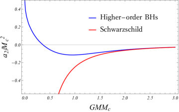
Figure 3: We plot $a_{2}/M_{c}^{2}$ as a function of the mass (interpolation) for $\lambda_{\geq 4}=0$, $\lambda_{3}=1$ and for the Schwarzschild solution, $a_{2}=-(2GM)^{-2}$ (red).

Appendix C (A)dS asymptotes and general horizon geometries

In the main text we have focused on static, spherically symmetric and asymptotically flat solutions. Our results can be easily extended to (A)dS asymptotes as well as to planar or hyperbolic horizon geometries. In particular (2) can be generalized to

$$\mathcal{L}=\frac{1}{16\pi G}\left[R-2\Lambda_{0}+\frac{\lambda_{2}}{M_{c}^{2}}\mathcal{X}_{4}+\sum_{n=3}^{\infty}\frac{\lambda_{n}}{M_{c}^{2(n-1)}}\mathcal{R}_{(n)}\right]\,,$$ (29)

where we have now made explicit the topological Gauss-Bonnet term $\mathcal{X}_{4}=R^{2}-4R_{ab}R^{ab}+R_{abcd}R^{abcd}$, which we will use to impose the entropy to vanish as $M\rightarrow 0$. We can search for solutions of the form

$$ds^{2}=-f(r)dt^{2}+\frac{dr^{2}}{f(r)}+r^{2}d\Sigma_{(k)}^{2}\,,$$ (30)

where $d\Sigma_{(k)}^{2}$ is the metric of a 2-dimensional maximally symmetric space of curvature $k=1,0,-1$, i.e., , the metric of the unit sphere, flat space or hyperbolic space. The generalized version of the equation which determines the metric function $f(r)$ then reads (note that $M$ is no longer the mass in the planar and hyperbolic cases):

$$-(f-k)r-\sum_{n=3}^{\infty}\frac{\lambda_{n}}{M_{c}^{2n-2}}\left(\frac{f^{\prime}}{r}\right)^{n-3}\Bigg{[}\frac{f^{\prime 3}}{n}+\frac{(n-3)f+2k}{(n-1)r}f^{\prime 2}-\frac{2}{r^{2}}f(f-k)f^{\prime}-\frac{1}{r}ff^{\prime\prime}\left(f^{\prime}r-2(f-k)\right)\Bigg{]}$$ (31)

$$=2GM+\frac{1}{3}\Lambda_{0}r^{3}\,.$$

The generalized versions of equations (7) and (8) read

$$2GM-kr_{h}+\frac{1}{3}\Lambda_{0}r_{h}^{3} =-4\pi T\sum_{n=3}^{\infty}\frac{\lambda_{n}}{M_{c}^{2n-2}}\left(\frac{4\pi T}{r_{h}}\right)^{n-2}\left(\frac{4\pi Tr_{h}}{n}+\frac{2k}{n-1}\right)\,,$$ (32)

$$k-r_{h}^{2}\Lambda_{0} =+4\pi Tr_{h}+\sum_{n=3}^{\infty}\frac{\lambda_{n}}{M_{c}^{2n-2}}\left(\frac{4\pi T}{r_{h}}\right)^{n-1}\frac{2nk+(n-3)4\pi Tr_{h}}{n(n-1)}\,.$$ (33)

Wald’s entropy reads in turn

$$\mathsf{S}=\frac{\pi r_{h}^{2}}{G}\left[1-2\sum_{n=3}^{\infty}\frac{\lambda_{n}}{M_{c}^{2n-2}}\left(\frac{4\pi T}{r_{h}}\right)^{n-1}\left(\frac{2k}{(n-2)4\pi Tr_{h}}+\frac{1}{n-1}\right)\right]+\frac{2\pi k\lambda_{2}}{GM_{c}^{2}}\,.$$ (34)

Appendix D Linearized equations

We can obtain the embedding equation of a maximally symmetric background of curvature $\Lambda$ by plugging $f(r)=k-\Lambda r^{2}$ in (C) with $M=0$. Then we get the equation

$$\Lambda+M_{c}^{2}\sum_{n=3}^{\infty}\frac{\lambda_{n}(-1)^{n}}{n(n-1)}\left(\frac{2\Lambda}{M_{c}^{2}}\right)^{n}=\frac{1}{3}\Lambda_{0}\,,$$ (35)

which determines the possible vacua of the theory. For any of them, we know that the theory only propagates a massless graviton, due to the results in Bueno and Cano (2017). Thus, the linearized equations satisfied by a metric perturbation $h_{ab}$ over a maximally symmetric background $\bar{g}_{ab}$, read simply

$$G_{ab}^{L}=8\pi G_{\rm eff}T_{ab}\,,$$ (36)

where $G_{ab}^{L}$ is the linearized Einstein tensor,

$$G_{ab}^{L} =R_{ab}^{L}-\frac{1}{2}\bar{g}_{ab}R^{L}-(D-1)\Lambda h_{ab}\,,$$ (37)

$$R_{ab}^{L} =\bar{\nabla}_{(a|}\bar{\nabla}_{c}h^{c}_{\ |b)}-\frac{1}{2}\bar{\Box}h_{ab}-\frac{1}{2}\bar{\nabla}_{a}\bar{\nabla}_{b}h+D\Lambda h_{ab}-\Lambda h\bar{g}_{ab}\,,$$ (38)

$$R^{L} =\bar{\nabla}^{a}\bar{\nabla}^{b}h_{ab}-\bar{\Box}h-(D-1)\Lambda h\,,$$ (39)

and where the effective gravitational constant $G_{\rm eff}$ reads

$$G_{\rm eff}=\frac{G}{1+2\sum_{n=3}^{\infty}\frac{\lambda_{n}(-1)^{n}}{n-1}\left(\frac{2\Lambda}{M_{c}^{2}}\right)^{n-1}}\,.$$ (40)

Observe that, for theories with Einstein-like spectrum, this can be generically obtained by using the fact that $G/G_{\rm eff}$ is the slope of the lhs of (35) evaluated on the background Bueno and Cano (2016a); Bueno et al. (2017). Finally, in the transverse gauge, $\bar{\nabla}_{a}h^{ab}=\bar{\nabla}^{b}h$, we can write

$$-\bar{\Box}h_{ab}=16\pi G_{\rm eff}T_{ab}\,.$$ (41)

References

- Hawking (1975) S. W. Hawking, In *Gibbons, G.W. (ed.), Hawking, S.W. (ed.): Euclidean quantum gravity* 167-188, Commun. Math. Phys. 43, 199 (1975), [,167(1975)].
- Schwarzschild (1916) K. Schwarzschild, Sitzungsber. Preuss. Akad. Wiss. Berlin (Math. Phys.) 1916, 189 (1916), arXiv:physics/9905030 [physics] .
- Harlow (2016) D. Harlow, Rev. Mod. Phys. 88, 15002 (2016), [Rev. Mod. Phys.88,15002(2016)], arXiv:1409.1231 [hep-th] .
- Chen et al. (2015) P. Chen, Y. C. Ong, and D.-h. Yeom, Phys. Rept. 603, 1 (2015), arXiv:1412.8366 [gr-qc] .
- Myers (1997) R. C. Myers, Gen. Rel. Grav. 29, 1217 (1997), arXiv:gr-qc/9705065 [gr-qc] .
- Nepomechie (1985) R. I. Nepomechie, Phys. Rev. D32, 3201 (1985).
- Gross and Witten (1986) D. J. Gross and E. Witten, Nucl. Phys. B277, 1 (1986).
- Gross and Sloan (1987) D. J. Gross and J. H. Sloan, Nucl. Phys. B291, 41 (1987).
- ’t Hooft and Veltman (1974) G. ’t Hooft and M. J. G. Veltman, Ann. Inst. H. Poincare Phys. Theor. A20, 69 (1974).
- Deser and van Nieuwenhuizen (1974) S. Deser and P. van Nieuwenhuizen, Phys. Rev. D10, 401 (1974).
- Myers and Simon (1988) R. C. Myers and J. Z. Simon, Phys. Rev. D38, 2434 (1988).
- Myers and Simon (1989) R. C. Myers and J. Z. Simon, Gen. Rel. Grav. 21, 761 (1989).
- Callan et al. (1989) C. G. Callan, Jr., R. C. Myers, and M. J. Perry, Nucl. Phys. B311, 673 (1989).
- Lu et al. (2015a) H. Lu, A. Perkins, C. N. Pope, and K. S. Stelle, Phys. Rev. D92, 124019 (2015a), arXiv:1508.00010 [hep-th] .
- Lu et al. (2015b) H. Lu, A. Perkins, C. N. Pope, and K. S. Stelle, Phys. Rev. Lett. 114, 171601 (2015b), arXiv:1502.01028 [hep-th] .
- de la Cruz-Dombriz et al. (2009) A. de la Cruz-Dombriz, A. Dobado, and A. L. Maroto, Phys. Rev. D80, 124011 (2009), [Erratum: Phys. Rev.D83,029903(2011)], arXiv:0907.3872 [gr-qc] .
- Riegert (1984) R. J. Riegert, Phys. Rev. Lett. 53, 315 (1984).
- Klemm (1998) D. Klemm, Class. Quant. Grav. 15, 3195 (1998), arXiv:gr-qc/9808051 [gr-qc] .
- Bueno et al. (2016) P. Bueno, P. A. Cano, A. O. Lasso, and P. F. Ramirez, JHEP 04, 028 (2016), arXiv:1602.07310 [hep-th] .
- Cai et al. (2009a) R.-G. Cai, Y. Liu, and Y.-W. Sun, JHEP 10, 080 (2009a), arXiv:0909.2807 [hep-th] .
- Lovelock (1970) D. Lovelock, aequationes mathematicae 4, 127 (1970).
- Lovelock (1971) D. Lovelock, J. Math. Phys. 12, 498 (1971).
- Boulware and Deser (1985) D. G. Boulware and S. Deser, Phys. Rev. Lett. 55, 2656 (1985).
- Wheeler (1986) J. T. Wheeler, Nucl. Phys. B273, 732 (1986).
- Cai (2002) R.-G. Cai, Phys. Rev. D65, 084014 (2002), arXiv:hep-th/0109133 [hep-th] .
- Dehghani and Pourhasan (2009) M. H. Dehghani and R. Pourhasan, Phys. Rev. D79, 064015 (2009), arXiv:0903.4260 [gr-qc] .
- de Boer et al. (2010a) J. de Boer, M. Kulaxizi, and A. Parnachev, JHEP 06, 008 (2010a), arXiv:0912.1877 [hep-th] .
- Bueno and Cano (2016a) P. Bueno and P. A. Cano, Phys. Rev. D94, 104005 (2016a), arXiv:1607.06463 [hep-th] .
- Hennigar and Mann (2016) R. A. Hennigar and R. B. Mann, (2016), arXiv:1610.06675 [hep-th] .
- Bueno and Cano (2016b) P. Bueno and P. A. Cano, Phys. Rev. D94, 124051 (2016b), arXiv:1610.08019 [hep-th] .
- Hennigar et al. (2017) R. A. Hennigar, D. Kubiznak, and R. B. Mann, (2017), arXiv:1703.01631 [hep-th] .
- Bueno and Cano (2017) P. Bueno and P. A. Cano, (2017), arXiv:1703.04625 [hep-th] .
- Ahmed et al. (2017) J. Ahmed, R. A. Hennigar, R. B. Mann, and M. Mir, (2017), arXiv:1703.11007 [hep-th] .
- Myers and Robinson (2010) R. C. Myers and B. Robinson, JHEP 08, 067 (2010), arXiv:1003.5357 [gr-qc] .
- Bueno et al. (2017) P. Bueno, P. A. Cano, V. S. Min, and M. R. Visser, Phys. Rev. D95, 044010 (2017), arXiv:1610.08519 [hep-th] .
- Arnowitt et al. (1960a) R. L. Arnowitt, S. Deser, and C. W. Misner, Phys. Rev. 117, 1595 (1960a).
- Arnowitt et al. (1960b) R. Arnowitt, S. Deser, and C. W. Misner, Phys. Rev. 118, 1100 (1960b).
- Arnowitt et al. (1961) R. L. Arnowitt, S. Deser, and C. W. Misner, Phys. Rev. 122, 997 (1961).
- Wald (1993) R. M. Wald, Phys. Rev. D48, 3427 (1993), arXiv:gr-qc/9307038 [gr-qc] .
- Maldacena (1999) J. M. Maldacena, Int. J. Theor. Phys. 38, 1113 (1999), [Adv. Theor. Math. Phys.2,231(1998)], arXiv:hep-th/9711200 [hep-th] .
- Witten (1998) E. Witten, Adv. Theor. Math. Phys. 2, 253 (1998), arXiv:hep-th/9802150 [hep-th] .
- Gubser et al. (1998) S. S. Gubser, I. R. Klebanov, and A. M. Polyakov, Phys. Lett. B428, 105 (1998), arXiv:hep-th/9802109 [hep-th] .
- Easson (2003) D. A. Easson, JHEP 02, 037 (2003), arXiv:hep-th/0210016 [hep-th] .
- Aharonov et al. (1987) Y. Aharonov, A. Casher, and S. Nussinov, Phys. Lett. B191, 51 (1987).
- Preskill (1992) J. Preskill, in International Symposium on Black holes, Membranes, Wormholes and Superstrings Woodlands, Texas, January 16-18, 1992 (1992) pp. 22–39, arXiv:hep-th/9209058 [hep-th] .
- Harvey and Strominger (1993) J. A. Harvey and A. Strominger, in Theoretical Advanced Study Institute (TASI 92): From Black Holes and Strings to Particles Boulder, Colorado, June 3-28, 1992 (1993) pp. 537–588, [,122(1992)], arXiv:hep-th/9209055 [hep-th] .
- Giddings (1995) S. B. Giddings, Phys. Rev. D51, 6860 (1995), arXiv:hep-th/9412159 [hep-th] .
- Susskind (1995) L. Susskind, (1995), arXiv:hep-th/9501106 [hep-th] .
- Giddings and Strominger (1992) S. B. Giddings and A. Strominger, Phys. Rev. D46, 627 (1992), arXiv:hep-th/9202004 [hep-th] .
- Callan et al. (1992) C. G. Callan, Jr., S. B. Giddings, J. A. Harvey, and A. Strominger, Phys. Rev. D45, R1005 (1992), arXiv:hep-th/9111056 [hep-th] .
- Giddings (1992) S. B. Giddings, Phys. Rev. D46, 1347 (1992), arXiv:hep-th/9203059 [hep-th] .
- Alvarez-Gaume et al. (2016) L. Alvarez-Gaume, A. Kehagias, C. Kounnas, D. Lust, and A. Riotto, Fortsch. Phys. 64, 176 (2016), arXiv:1505.07657 [hep-th] .
- Chen and Adler (2003) P. Chen and R. J. Adler, Sources and detection of dark matter and dark energy in the universe. Proceedings, 5th International Symposium, Dark Matter 2002, Marina del Rey, USA, February 20-22, 2002, Nucl. Phys. Proc. Suppl. 124, 103 (2003), [,103(2002)], arXiv:gr-qc/0205106 [gr-qc] .
- Afshordi et al. (2003) N. Afshordi, P. McDonald, and D. N. Spergel, Astrophys. J. 594, L71 (2003), arXiv:astro-ph/0302035 [astro-ph] .
- Nozari and Mehdipour (2005) K. Nozari and S. H. Mehdipour, Mod. Phys. Lett. A20, 2937 (2005), arXiv:0809.3144 [gr-qc] .
- Mureika (2012) J. R. Mureika, Phys. Lett. B716, 171 (2012), arXiv:1204.3619 [gr-qc] .
- Fulling et al. (1992) S. A. Fulling, R. C. King, B. G. Wybourne, and C. J. Cummins, Classical and Quantum Gravity 9, 1151 (1992).
- Deser and Ryzhov (2005) S. Deser and A. V. Ryzhov, Class. Quant. Grav. 22, 3315 (2005), arXiv:gr-qc/0505039 [gr-qc] .
- Cisterna et al. (2017) A. Cisterna, L. Guajardo, M. Hassaine, and J. Oliva, (2017), arXiv:1702.04676 [hep-th] .
- Brigante et al. (2008) M. Brigante, H. Liu, R. C. Myers, S. Shenker, and S. Yaida, Phys. Rev. D77, 126006 (2008), arXiv:0712.0805 [hep-th] .
- de Boer et al. (2010b) J. de Boer, M. Kulaxizi, and A. Parnachev, JHEP 03, 087 (2010b), arXiv:0910.5347 [hep-th] .
- Camanho and Edelstein (2010a) X. O. Camanho and J. D. Edelstein, JHEP 04, 007 (2010a), arXiv:0911.3160 [hep-th] .
- Buchel and Myers (2009) A. Buchel and R. C. Myers, JHEP 08, 016 (2009), arXiv:0906.2922 [hep-th] .
- Cai et al. (2009b) R.-G. Cai, Z.-Y. Nie, N. Ohta, and Y.-W. Sun, Phys. Rev. D79, 066004 (2009b), arXiv:0901.1421 [hep-th] .
- Camanho and Edelstein (2010b) X. O. Camanho and J. D. Edelstein, JHEP 06, 099 (2010b), arXiv:0912.1944 [hep-th] .
- Buchel et al. (2010) A. Buchel, J. Escobedo, R. C. Myers, M. F. Paulos, A. Sinha, and M. Smolkin, JHEP 03, 111 (2010), arXiv:0911.4257 [hep-th] .
- Myers et al. (2010) R. C. Myers, M. F. Paulos, and A. Sinha, JHEP 08, 035 (2010), arXiv:1004.2055 [hep-th] .
- Holdom and Ren (2016) B. Holdom and J. Ren, (2016), arXiv:1612.04889 [gr-qc] .