Loss Max-Pooling for Semantic Image Segmentation
Abstract
We introduce a novel loss max-pooling concept for handling imbalanced training data distributions, applicable as alternative loss layer in the context of deep neural networks for semantic image segmentation. Most real-world semantic segmentation datasets exhibit long tail distributions with few object categories comprising the majority of data and consequently biasing the classifiers towards them. Our method adaptively re-weights the contributions of each pixel based on their observed losses, targeting under-performing classification results as often encountered for under-represented object classes. Our approach goes beyond conventional cost-sensitive learning attempts through adaptive considerations that allow us to indirectly address both, inter- and intra-class imbalances. We provide a theoretical justification of our approach, complementary to experimental analyses on benchmark datasets. In our experiments on the Cityscapes and Pascal VOC 2012 segmentation datasets we find consistently improved results, demonstrating the efficacy of our approach.
1 Introduction
Deep learning approaches have undoubtedly matured to the new de facto standards for many traditional computer vision tasks like image classification, object detection or semantic segmentation. Semantic segmentation aims to assign categorical labels to each pixel in an image and therefore constitutes the basis for high-level image understanding. Recent works have contributed to the progress in this research field by building upon convolutional neural networks (CNNs) [30] and enriching them with task-specific functionalities. Extending CNNs to directly cast dense, semantic label maps [34, 2], including more contextual information [33, 9, 46, 16] or refining results with graphical models [31, 47], have led to impressive results in many real-world applications and on standard benchmark datasets.
Few works have focused on how to properly handle imbalanced (or skewed) class distributions, as often encountered in semantic segmentation datasets, within deep neural network training so far. With imbalanced, we refer to datasets having dominant portions of their data assigned to (few) majority classes while the rest belongs to minority classes, forming comparably under-represented categories. As (mostly undesired) consequence, it can be observed that classifiers trained without correction mechanisms tend to be biased towards the majority classes during inference.
One way to mitigate this class-imbalance problem is to emphasize on balanced compilations of datasets in the first place by collecting their samples approximately uniformly. Datasets following such an approach are ImageNet [11], Caltech 101/256 [15, 17] or CIFAR 10/100 [29], where training, validation and test sets are roughly balanced w.r.t. the instances per class. Another widely used procedure is conducting over-sampling of minority classes or under-sampling from the majority classes when compiling the actual training data. Such approaches are known to change the underlying data distributions and may result in suboptimal exploitation of available data, increased computational effort and/or risk of over-fitting when repeatedly visiting the same samples from minority classes (c.f. SMOTE and derived variants [8, 19, 6, 24] on ways to avoid over-fitting). However, its efficiency and straightforward application for tasks like image-level classification rendered sampling a commonly-agreed practice.
Another approach termed cost-sensitive learning changes the algorithmic behavior by introducing class-specific weights, often derived from the original data statistics. Such methods were recently investigated [44, 45, 35, 7] for deep learning, some of them following ideas previously applied in shallow learning methods like random forests [27, 28] or support vector machines [38, 42]. Many of these works use statically-defined cost matrices [44, 12, 45, 35, 7] or introduce additional parameter learning steps [26]. Due to the spatial arrangement and strong correlations of classes between adjacent pixels, cost-sensitive learning techniques are preferred over resampling methods when performing dense, pixel-wise classification as in semantic segmentation tasks. However, current trends of semantic segmentation datasets show strong increase in complexity with more minority classes being added.
Contributions. In this work we propose a principled solution to handling imbalanced datasets within deep learning approaches for semantic segmentation tasks. Specifically, we introduce a novel loss function, which upper bounds the traditional losses where the contribution of each pixel is weighted equally. The upper bound is obtained via a generalized max-pooling operator acting at the pixel-loss level. The maximization is taken with respect to pixel weighting functions, thus providing an adaptive re-weighting of the contributions of each pixel, based on the loss they actually exhibit. In general, pixels incurring higher losses during training are weighted more than pixels with a lower loss, thus indirectly compensating potential inter-class and intra-class imbalances within the dataset. The latter imbalance is approached because our dynamic re-weighting is class-agnostic, i.e. we are not taking advantage of the class label statistics like previous cost-sensitive learning approaches.
The generalized max-pooling operator, and hence our new loss, can be instantiated in different ways depending on how we delimit the space of feasible pixel weighting functions. In this paper, we focus on a particular family of weighting functions with bounded -norm and -norm, and study the properties that our loss function exhibits under this setting. Moreover, we provide the theoretical contribution of deriving an explicit characterization of our loss function under this special case, which enables the computation of gradients that are needed for the optimization of the deep neural network.
As additional, complementary contribution we describe a performance-dependent sampling approach, guiding the minibatch compilation during training. By keeping track of the prediction performance on the training set, we show how a relatively simple change in the sampling scheme allows us to faster reach convergence and improved results.
The rest of this section discusses some related works and how current semantic segmentation approaches typically deal with the class-imbalance problem, before we provide a compact description for the notation used in the rest of this paper. In Sect. 2 we describe how we depart from the standard, uniform weighting scheme to our proposed adaptive, pixel-loss max-pooling and the space of weighting functions we are considering. Sect. 3 and 4 describe how we eventually solve the novel loss function and provide algorithmic details, respectively. In Sect. 5 we assess the performance of our contributions on the challenging Cityscapes and Pascal VOC segmentation benchmarks before we conclude in Sect. 6. Note that this is an extended version of our CVPR 2017 paper [39].
Related Works. Many semantic segmentation works follow a relatively simple cost-sensitive approach via an inverse frequency rebalancing scheme, e.g. [44, 45, 35, 7] or median frequency re-weighting [12]. Other approaches construct best-practice heuristics by e.g. restricting the number of pixels to be updated during backpropagation: The work in [3] suggests increasing the minibatch size while decreasing the absolute number of (randomly sampled) pixel positions to be updated. In [43], an approach coined online bootstrapping is introduced, where pixel losses are sorted and only the k highest loss positions are updated. A similar idea termed online hard example mining [41] was found to be effective for object detection, where high-loss bounding boxes retained after a non-maximum-suppression step were preferably updated. The work in [23] tackles class imbalance via enforcing inter-cluster and inter-class margins, obtained by employing quintuplet instance sampling with a triple-header hinge loss. Another recent work [26] proposed a cost-sensitive neural network for classification, jointly optimizing for class dependent costs and the standard neural network parameters. The work in [40] addresses the problem of contour detection with convolutional neural networks (CNN), combining a specific loss for contour versus non-contour samples with the conventional log-loss. In separate though related research fields, focus was put on directly optimizing the target measures like Area under curve (AUC), Intersection over Union (IoU or Jaccard Index) or Average class (AC) [4, 37, 36, 1]. The work in [18] is proposing a nonlinear activation function computing the norm of projections from the lower layers, allowing to interpret max-, average- and root-mean-squared-pooling operators as special cases of their activation function.
Notation. In this paper, we denote by the space of functions mapping elements in the set to elements in the set , while with a natual number denotes the usual product set of -tuples with elements in . The sets of real and integer numbers are and , respectively. Let , . Operations defined on such as, e.g. addition, multiplication, exponentiation, etc., are inherited by via pointwise application (for instance, is the function and is the function ). Additionally, we use the notations:
-
•
, and
-
•
and
-
•
-
•
-
•
denotes the function .
2 Pixel-Loss Max-Pooling
The goal of semantic image segmentation is to provide an assignment of class labels to each pixel of an image. The input space for this task is denoted by and corresponds to the set of possible images. For the sake of simplicity, we assume all images to have the same number of pixels . We denote by the set of pixels within an image, and let be the number of pixels, i.e. . The output space for the segmentation task is denoted by and corresponds to all pixelwise labelings with classes in . Each labeling is a function mapping pixels to classes, i.e. .
Standard setting. The typical objective used to train a model with parameters (e.g. a fully-convolutional network), given a training set , takes the following form:
| (1) |
where is the set of possible network parameters, is a loss function penalizing wrong image labelings and is a regularizer. The loss function commonly decomposes into a sum of pixel-specific losses as follows
| (2) |
where assigns to each pixel the loss incurred for predicting class instead of . In the rest of the paper, we assume to be non-negative and bounded (i.e. pixel losses are finite).
Loss max-pooling. The loss function defined in (2) weights uniformly the contribution of each pixel within the image. The effect of this choice is a bias of the learner towards elements that are dominant within the image (e.g. sky, building, road) to the detriment of elements occupying smaller portions of the image. In order to alleviate this issue, we propose to adaptively reweigh the contribution of each pixel based on the actual loss we observe. Our goal is to shift the focus on image parts where the loss is higher, while retaining a theoretical link to the loss in (2). The solution we propose is an upper bound to , which is constructed by relaxing the pixel weighting scheme. In general terms, we design a convex, compact space of weighting functions , subsuming the uniform weighting function, i.e. , and parametrize the loss function in (2) as
| (3) |
with . Then, we define a new loss function , which targets the highest loss incurred with a weighting function in , i.e.
| (4) |
Since the uniform weighting function belongs to and we maximize over , it follows that upper bounds , i.e. for any . Consequently, we obtain an upper bound to (1) if we replace by .
The title of our work, which ties the loss to max-pooling, is inspired by the observation that the loss proposed in (4) is the application of a generalized max-pooling operator acting on the pixel-losses. Indeed, we recover a conventional max-pooling operator as a special case if is the set of probability distributions over . Similarly, the standard loss in (2) can be regarded as the application of an average-pooling operator, which again can be boiled down to a special case of (4) under a proper choice of .
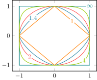
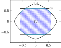
The space of weighting functions. The property that the loss max-pooling operator exhibits depends on the shape of . Here, we restrict the focus to weighting functions with -norm ( and -norm upper bounded by and , respectively (see Fig. 1 for an example):
| (5) |
We fix the bound on the -norm to with , which corresponds to the -norm of a uniform weighting function. Instead, and are left as hyper-parameters. Possible values of should be chosen in the range [. Indeed, lower values would prevent the uniform weighting function from belonging to , while higher values would be equivalent to putting .
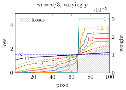
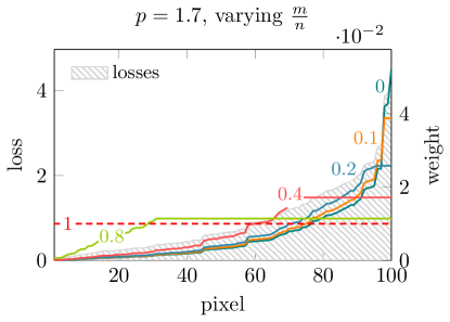
Intuitively, the user can control the pixel selectivity degree of the pooling operation in (4) by changing . Indeed, the optimal weights will be in general concentrated around a single pixel as and be uniformly spread across pixels as . On the other hand, allows to control, through the relation , the minimum number of pixels (namely ) that should be supported by the optimal weighting function. In Fig. 2 we show some examples, given synthetically-generated losses for pixels (sorted for better visualization). On the left, we fix (i.e. at least of the pixels should be supported) and report the optimal weightings for different values of . As we can see, the weights get more peaked on high losses as moves towards , but the constraint on prevents selecting less than pixels. On the other hand, the weights tend to become uniform as approaches . The plot on the right fixes and varies . We see that the weights tend to uniformly support a larger share of pixels as we increase , yielding the uniform distribution when .
3 Computation of
The maximization problem in (4) is concave and has an explicit-form solution if is defined as in (5). We provide the details by cases, considering the parametrization in place of , because has a clear intuitive meaning as mentioned in the previous section. Valid parametrizations satisfy and .
3.1 Case
To address this case, we consider the following dual formulation of the maximization problem in (4):
| (6) |
where is the dual variable accounting for the constraint , which is equivalent to , and
Moving from the primal to the dual formulation is legitimate because both formulations share the same optimal value. Indeed, the Slater’s condition applies [5] (e.g. function is strictly feasible).
The maximization in is the definition of the dual norm [5, Appendix A.1.6] of the -norm, which corresponds to the -norm with , evaluated in and scaled by . Accordingly, we have that
| (7) |
We get a solution to (6) by finding a point that satisfies
| (8) |
and maximizes (see, Prop. 3 in the appendix). However, computing such a solution from (8) is not straightforward due to the recursive nature of the formula involving multiple variables (elements of ). We reduce it to the problem of finding the largest root of the single-variable function
| (9) |
where and is its complement. This characterization of solutions to the dual formulation (6) in terms of roots of is proved correct in the appendix (Prop. 1) and it is used to derive the theorem below, which provides an explicit formula for , the optimal weighting function of the maximization in (4) and the optimal dual variable :
3.2 Case
For this case, the solution takes the same form as in (10), but becomes the subset of pixels with the highest losses, while is the highest loss among the remaining pixels ( if ). As for the optimal weighting function , let . Then for any probability distribution over
is an optimal solution for the primal (see, Thm. 2 in the appendix).
4 Algorithmic Details
The key quantities to compute are and . Indeed, once those are available we can determine the loss and compute gradients with respect to the segmentation model’s parameters (we show it later in this section). We report in Algorithm 1 the pseudo-code of the computation of and . We start sorting the losses (line 1). This yields a bijective function satisfying if (we wrote for ). Case (line 13) is trivial, since we know that the last ranked pixels will form , while corresponds to the highest loss among the remaining pixels, or if no pixel is left (see, Subsection 3.2). As for case , we walk through the losses in ascending order and stop as soon as we find an index satisfying one of the following conditions: a) and , or b) . If the first condition is hit, then and, hence, . This is indeed what we obtain in line 11, where so that , where and . Instead, if condition b is hit, then we have by Prop. 10 in the appendix that . Consequently, and so that .
Gradient. In order to train the semantic segmentation model we need to compute the partial derivative . It exists almost everywhere111Precisely, it exists in all having an open neighborhood where does not change. and is given by (see derivations in the appendix)
Note that we will use the same function also where the partial derivative technically does not exist.222This is a common practice within the deep learning community (see, e.g. how the derivative of ReLU, or max-pooling, are computed).
Implementation notes. For values of close to 1, we have that becomes arbitrarily large and this might cause numerical issues in Algorithm 1. A simple trick to improve stability consists in normalizing the losses with a division by the maximum loss, i.e. we consider in place of . This modification then requires multiplying by to adjust the objective, while the optimal primal solution remains unaffected by the change.
Complimentary sampling strategy. In addition to our main contribution described in the previous sections, we propose a complimentary idea on how to compile minibatches during training. We propose a mixed sampling approach taking both, uniform sampling from the training data’s global distribution and the current performance of the model into account. As a surrogate for the latter, we keep track of the per-class Intersection over Union (IoU) scores on the training data and conduct inverse sampling, which will suggest to preferably pick from under-performing classes (that are often strongly correlated with minority classes). Blending this performance-based sampling idea with uniform sampling ensures to maintain stochastic behavior during training and therefore helps not to over-fit to particular classes.
5 Experiments
We have evaluated our novel loss max-pooling (LMP) approach on the Cityscapes [10] and the extended Pascal VOC [14] semantic image segmentation datasets. In particular, we have performed an extensive parameter sweep on Cityscapes, assessing the performance development for different settings of our hyper-parameters and (see Equ. (5) and Fig. 2). All reported numbers are Intersection-over-Union (IoU) (or Jaccard) measures in , either averaged over all classes or provided on a per-class basis.
5.1 Network architecture
For all experiments, we are using a network architecture similar to the one of DeepLabV2 [9], implemented within Caffe [25] using cuDNN for performance improvement and NCCL333https://github.com/NVIDIA/nccl for multi-GPU support. In particular, we are using ResNet-101 [21] in a fully-convolutional way with atrous extensions [22, 46] for the base layers before adding DeepLab’s atrous spatial pyramid pooling (ASPP). Finally, we apply upscaling (via deconvolution layers with fixed, uniform weights and therefore performing bilinear upsampling) before using standard softmax loss for all baseline methods BASE, BASE+ and for the inverse median frequency weighting [12] while we use our proposed loss max-pooling layer in LMP. Both our approaches, BASE+ and LMP are using the complimentary sampling strategy for minibatch compilation as described in the previous section, while plain uniform sampling in BASE leads to similar results as reported in [9]. We also report results of our new loss with plain uniform sampling (“Proposed loss only”). To save computation time and provide a conclusive parameter sensitivity study for our approach, we disabled both, multi-scale input to the networks and post processing via conditional random fields (CRF). We consider both of these features as complementary to our method and highly relevant for improving the overall performance in case time and hardware budgets permit to do so. However, our primary intention is to demonstrate the effectiveness of our LMP, under comparable settings with other baselines like our BASE+. All our reported numbers and plots are obtained from fine-tuning the MS-COCO [32] pre-trained CNN of [9], which is available for download444http://liangchiehchen.com/projects/DeepLabv2_resnet.html. In order to provide statistically more significant results, we provide mean and standard deviations obtained by averaging the results at certain steps over the last 30k training iterations. We only report results obtained from a single CNN as opposed to using an ensemble of CNNs, trained using the stochastic gradient descent (SGD) solver with polynomial decay of the learning rate (”poly” as described in [9]) setting both, decay rate and momentum to . For data augmentation (Augm.), we use random scale perturbations in the range for patches cropped at positions given by the aforementioned sampling strategy, and horizontal flipping of images.
5.2 Cityscapes
This recently-released dataset contains street-level images, taken at daytime from driving scenes in 50 major central European cities in Germany, France and Switzerland. Images are captured at high resolution (2.048 1.024) and are divided into training, validation and test sets holding 2.975, 500 and 1.525 images, respectively. For training and validation data, densely annotated ground truth into 20 label categories (19 objects + ignore) is publicly available, where the 6 most frequent classes account for 90% of the annotated pixel mass. Following previous works [9, 43], we report results obtained on the validation set. During training, we use minibatches comprising 2 image crops, each of size . The initial learning rate is set to , and we run a total number of training iterations.
| 150k | 160k | 165k | Mean | Std.Dev. | |
|---|---|---|---|---|---|
| 1.0 | 74,35 | 74.64 | 74.64 | 74.54 | 0.17 |
| 1.1 | 74.34 | 74.61 | 74.60 | 74.52 | 0.15 |
| 1.2 | 74.42 | 74.60 | 74.77 | 74.60 | 0.18 |
| 1.3 | 74.52 | 74.71 | 74.69 | 74.64 | 0.10 |
| 1.4 | 74.33 | 74.51 | 74.49 | 74.44 | 0.10 |
| 1.5 | 74.03 | 73.99 | 74.04 | 74.02 | 0.03 |
| 1.6 | 74.05 | 74.42 | 74.52 | 74.33 | 0.25 |
| 1.7 | 74.10 | 74.56 | 74.74 | 74.57 | 0.17 |
| 1.8 | 73.65 | 74.18 | 74.17 | 74.00 | 0.30 |
| 1.9 | 73.97 | 74.21 | 74.48 | 74.22 | 0.26 |
| 2.3 | 73.93 | 74.23 | 74.12 | 74.09 | 0.15 |
| BASE+ | 73.12 | 73.16 | 73.10 | 73.13 | 0.03 |
In Tab. 1, we provide a sensitivity analysis for hyper-parameter , fixing to 25% of non-ignore per-crop pixels. Due to the large resolution of images and considerable number of trainings to be run, we employ different tiling strategies during inference. Numbers in Tab. 1 are obtained by using our so-called efficient tiling strategy, dividing the validation images into five non-overlapping, rectangular crops with full image height. With this setting, the best result was obtained for , closely followed by . It can be seen that increasing values for show a trend towards BASE+ results, empirically confirming the theoretical underpinnings from Sect. 2. After fixing , we conducted additional experiments with selected in a way to correspond to selecting at least , or of non-ignore per-crop pixels, obtaining and on the validation data, respectively. Finally, we locked in on and , running an optimized tiling strategy on the validation set where we consider a 200 pixel overlap between tiles, allowing for improved context capturing. The final class label decisions for the first half of the overlap area are then exclusively taken by the left tile while the second half is provided by the right tile, respectively. The resulting scores are listed in Tab. 2, demonstrating improved results over BASE, BASE+ and related approaches like DeepLabV2 [9] (even when using CRF) or [43] with deeper ResNet and online bootstrapping (BS). Also our loss alone, i.e. without the complimentary sampling strategy, yields improved results over both BASE and BASE+.
| Method | mean IoU |
|---|---|
| [9] RN-101 & Augm. & ASPP | 71.0 |
| [9] RN-101 & Augm. & ASPP & CRF | 71.4 |
| [43] FCRN-101 & Augm. | 71.16 |
| [43] FCRN-152 & Augm. | 71.51 |
| [43] FCRN-152 & Online BS & Augm. | 74.64 |
| Our approaches - Resnet-101 | |
| BASE Augm. & ASPP | 72.55 |
| BASE+ Augm. & ASPP | 73.63 |
| [12] Inverse median freq. & Augm. & ASPP | 69.81 |
| Proposed loss only & Augm. & ASPP | 74.17 |
| LMP Augm. & ASPP | 75.06 |
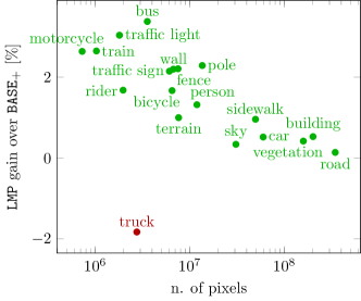
To demonstrate the impact of our approach on under-represented classes, we provide a plot showing the per-class performance gain (LMP- BASE+ on -axis in %) vs. the absolute number of pixels for a given object category (-axis, log-scale) in Fig. 3. Positive values on indicate improvements (18/19 classes) and class labels attached to indicate increasing object class pixel label volume for categories from left to right. E.g., motorcycle is most underrepresented while road is most present. The plot confirms how LMP naturally improves on underrepresented object classes without accessing the underlying class statistics.
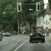
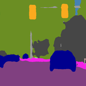
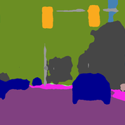
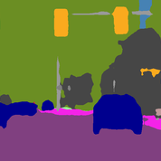
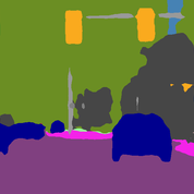
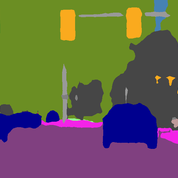
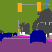
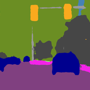
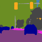
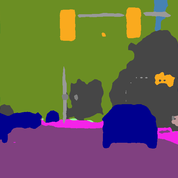
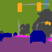
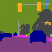
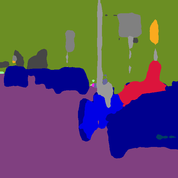
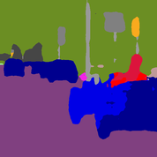
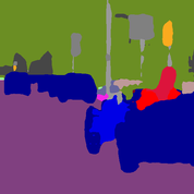
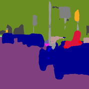
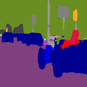
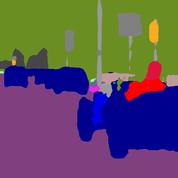
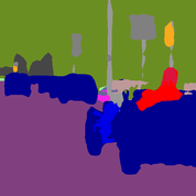
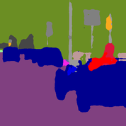
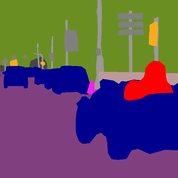
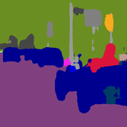
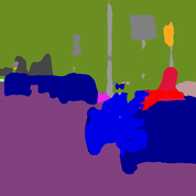
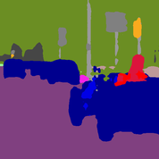
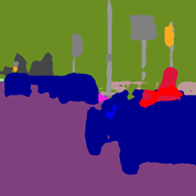
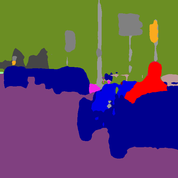
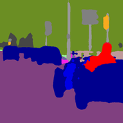
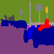
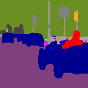
Another experiment we have run compares BASE to LMP: In order to match the result of LMP, one has to e.g. improve the worst 7 categories by 5% each or the worst 10 categories by 3% each, which we find a convincing argument for LMP. Additionally, we illustrate the qualitative evolution of the semantic segmentation for two training images in Fig. 4. Odd rows show segmentations obtained when training with conventional log-loss in BASE+, while even rows show the ones obtained using our loss max-pooling LMP at an increasing number of iterations. As we can see, LMP starts improving on under-represented classes sooner than standard log-loss (see, e.g. traffic light and its pole on the middle right in the first image, and the car driver in the second image).
 |
 |
 |
 |
 |
 |
 |
 |
 |
|
 |
 |
 |
 |
 |
 |
 |
 |
 |
|
 |
 |
 |
 |
 |
 |
 |
 |
 |
|
 |
 |
 |
 |
 |
 |
 |
 |
 |
Finally, we also report the individual per-class IoU scores in Tab. 3 for both, BASE+ and LMP, corresponding to the setting from Tab. 2.
| Method | Road | Sidewalk | Building | Wall | Fence | Pole | Traffic Light | Traffic Sign | Vegetation | Terrain | Sky | Person | Rider | Car | Truck | Bus | Train | Motorcycle | Bicycle | Mean |
|---|---|---|---|---|---|---|---|---|---|---|---|---|---|---|---|---|---|---|---|---|
| BASE+ Mean | 97.37 | 80.60 | 90.99 | 53.23 | 54.67 | 56.72 | 63.29 | 72.62 | 91.19 | 59.85 | 93.46 | 78.59 | 59.08 | 93.41 | 68.94 | 80.49 | 67.77 | 62.51 | 74.09 | 73.63 |
| BASE+ Std.Dev. | 0.01 | 0.02 | 0.14 | 0.92 | 0.05 | 0.08 | 0.56 | 0.13 | 0.13 | 0.96 | 0.16 | 0.18 | 0.31 | 0.12 | 0.26 | 1.08 | 3.12 | 0.70 | 0.11 | 0.04 |
| LMP Mean | 97.51 | 81.56 | 91.52 | 55.43 | 56.88 | 59.01 | 66.33 | 74.77 | 91.61 | 60.85 | 93.80 | 79.91 | 60.76 | 93.93 | 67.11 | 83.87 | 70.42 | 65.15 | 75.76 | 75.06 |
| LMP Std.Dev. | 0.05 | 0.32 | 0.06 | 0.80 | 0.68 | 0.31 | 0.27 | 0.21 | 0.07 | 0.27 | 0.09 | 0.08 | 0.29 | 0.01 | 0.77 | 0.44 | 0.53 | 0.44 | 0.14 | 0.09 |
| Method | Background | Aeroplane | Bicycle | Bird | Boat | Bottle | Bus | Car | Cat | Chair | Cow | Dining Table | Dog | Horse | Motorbike | Person | Potted Plant | Sheep | Sofa | Train | TV Monitor | Mean |
|---|---|---|---|---|---|---|---|---|---|---|---|---|---|---|---|---|---|---|---|---|---|---|
| BASE+ Mean | 92.69 | 83.21 | 78.46 | 81.39 | 67.95 | 77.59 | 92.14 | 80.17 | 86.99 | 38.49 | 80.86 | 55.95 | 81.03 | 80.64 | 79.28 | 81.14 | 61.74 | 81.51 | 47.76 | 82.25 | 72.68 | 75.42 |
| BASE+ Std.Dev. | 0.00 | 0.32 | 0.04 | 0.03 | 0.14 | 0.02 | 0.12 | 0.14 | 0.08 | 0.03 | 0.06 | 0.10 | 0.02 | 0.22 | 0.06 | 0.03 | 0.35 | 0.21 | 0.24 | 0.09 | 0.24 | 0.04 |
| LMP Mean | 92.84 | 85.02 | 79.62 | 81.43 | 69.99 | 76.36 | 92.38 | 82.38 | 89.43 | 39.78 | 82.70 | 58.60 | 82.85 | 81.82 | 80.17 | 81.60 | 61.22 | 84.30 | 45.44 | 82.52 | 71.70 | 76.29 |
| LMP Std.Dev. | 0.02 | 0.18 | 0.03 | 0.34 | 0.26 | 0.10 | 0.17 | 0.05 | 0.10 | 0.06 | 0.17 | 0.10 | 0.05 | 0.03 | 0.07 | 0.05 | 0.14 | 0.19 | 0.04 | 0.09 | 0.10 | 0.02 |
5.3 Pascal VOC 2012
We additionally assess the quality of our novel LMP on the Pascal VOC 2012 segmentation benchmark dataset [13], comprising 20 object classes and a background class. Images in this dataset are considerably smaller than the ones from the Cityscapes dataset so we increased the minibatch size to 4 (with crop sizes of ), using the (extended) training set with 10.582 images [20]. Testing was done on the validation set containing 1.449 images. We ran a total of 200k training iterations and fixed parameters and to account for of valid pixels per crop for our LMP. During inference, images are evaluated at full scale, i.e. no special tiling mechanism is needed. We again report the mean IoU scores in Tab. 4 (this time averaged after training iterations 180k, 190k and 200k), and list results from comparable state-of-the-art approaches [43, 9] next to ours.
| Method | mean IoU |
|---|---|
| [9] RN-101 Base w/o COCO | 68.72 |
| [9] RN-101 & MSC & Augm. & ASPP | 76.35 |
| [9] RN-101 & MSC & Augm. & ASPP & CRF | 77.69 |
| [43] FCRN-101 & Augm. | 73.41 |
| [43] FCRN-152 & Augm. | 73.32 |
| [43] FCRN-101 & Online BS & Augm. | 74.80 |
| [43] FCRN-152 & Online BS & Augm. | 74.72 |
| Our approaches - Resnet-101 | |
| BASE Augm. & ASPP | 75.74 |
| BASE+ Augm. & ASPP | 75.42 |
| [12] Inverse median freq. & Augm. & ASPP | 74.93 |
| Proposed loss only & Augm. & ASPP | 76.01 |
| LMP Augm. & ASPP | 76.29 |
We can again obtain a considerable relative improvement over BASE+ as well as comparable baselines from [43, 9]. Our approach compares slightly worse () with DeepLabV2’s strongest variant, which however additionally uses multi-scale inputs (MSC) and refinements from a CRF (contributing and according to [9], respectively) but only come with increased computational costs. Additionally, and as mentioned above, we consider both of these techniques as complementary to our contributions and plan to integrate them in future works. We finally notice that also for this dataset our new loss alone without the complimentary sampling strategy yields consistent improvements over BASE and BASE+.
In Tab. 3, we give side-by-side comparisons of per class IoU scores for BASE+ and LMP. Again, the majority of categories benefits from our approach, confirming its efficacy.
6 Conclusions
In this work we have introduced a novel approach to tackle imbalances in training data distributions, which do not occur only when we have under-represented classes (inter-class imbalance), but might occur also within the same class (intra-class imbalance). We proposed a new loss function that performs a generalized max-pooling of pixel-specific losses. Our loss upper bounds the traditional one, which gives equal weight to each pixel contribution, and implicitly introduces an adaptive weighting scheme that biases the learner towards under-performing image parts. The space of weighting functions involved in the maximization can be shaped to enforce some desired properties. In this paper we focused on a particular family of weighting functions, enabling us to control the pixel selectivity and the extent of the supported pixels. We have derived explicit formulas for the outcome of the pooling operation under this family of pixel weighting functions, thus enabling the computation of gradients for training deep neural networks. We have experimentally validated the effectiveness of our new loss function and showed consistently improved results on standard benchmark datasets for semantic segmentation.
Acknowledgements. We gratefully acknowledge financial support from project DIGIMAP, funded under grant #860375 by the Austrian Research Promotion Agency (FFG).
Appendix A Proofs and Auxiliary Results
Proof of Thm. 1.
Let and let . We start proving that . If , then by definition of we have , which implies by Proposition 8 (take and ). Consequently, and, therefore, . If , then by definition of we have , which implies since hold by Proposition 5. Therefore, . So, . We have thus proved that .
We obtain , as given in the theorem, by solving equation for variable , after having replaced with the equivalent . The equation admits a unique solution, because by Proposition 5. Accordingly, . Then, by Proposition 1 we have that is a solution to (6), from which we derive
As for , we have that holds in general. Now, if , then . If , then
where the last equality follows from the observation that , by definition of . Hence, is an optimal solution to the maximization in (4). ∎
Proposition 1.
Proof.
Theorem 2.
Let and . Then
| (11) |
where , i.e. contains the pixels with the highest losses, and , i.e. it corresponds to the highest loss in or zero if is empty. Moreover,
is an optimal solution for the maximization in (4), for any probability distribution defined over .
Proof.
Assume to be the maximizer in (4), i.e. . Then it has to be nonnegative and should satisfy . Otherwise, we could construct , which would satisfy contradicting .
Now, from (4) and the definition of we can derive
Assume by contradiction that strict inequality holds, or in other terms that . Let and . Note that and , otherwise holds yielding a contradiction, and , because is upper bounded by and for . It follows by definition of that for any . Additionally, , otherwise holds contradicting , and necessarily because is lower bounded by and for . It follows by definition of and that for any . But then
yielding a contradiction. Hence, , i.e. is an optimal solution for the maximization in (4), and (11) holds. ∎
Proposition 2.
Proof.
Let be a root of and let . By following the previous relation bottom-up, we obtain , and by substituting it back into we obtain (8). ∎
Proposition 3.
Proof.
Let be a solution to (6). If , then (8) is trivially satisfied. Otherwise, it is satisfied by Proposition 4.
Let . If , then is a solution to (6) by Proposition 4. If , then it is the only point satisfying (8). It follows from Proposition 4 that no solution to (6) exists where is differentiable. However, at least one solution has to exist because the minimization problem in (6) admits a finite solution. So, it has to be a point where is non-differentiable, but the only one is . Therefore, is a solution to (6). ∎
Proof.
() If is a solution to (6) and , then is a point where is differentiable and the Karush-Kuhn-Tucker (KKT) necessary conditions [5] for optimality are satisfied. Specifically, there exists satisfying
The complementarity constraint and the nonnegativity of imply that if . By using this fact, we can derive after simple algebraic manipulations the following equivalent relation, which holds for all :
and this corresponds to
Proposition 5.
Let and . If , then and , where .
Proof.
Let be a solution to (6). By Proposition 1 we have that is a root of . If we have and by Proposition 6 we have that has at most positive elements. It follows that . If , we have . This and imply . Accordingly, always holds and since , we have and .
Finally, assume by contradiction that holds. Then implies . Take , then , where . Let , which is necessarily non-empty and contains only pixels with loss . Then
where the last equality follows from the fact that for all . However, implies by definition of , which yields a contradiction because follows from the definition of . Hence, . ∎
Proposition 6.
Let and . If is a minimizer of (6), then has at most positive elements.
Proof.
If then and the result is trivially true. Otherwise (), assume by contradiction that there exist at least positive elements in , say with indices in . Then, the dual objective yields . However, this value cannot be attained by the primal formulation because there exist at most elements in with weight , while the remaining element would have a weight not exceeding (due to the constraint ). This implies , which contradicts strong duality, implied by the satisfaction of the Slater’s condition [5]. ∎
Proposition 7.
Let and . If , and , then , where .
Proof.
Let . The hypothesis implies that . Hence, we can write
where and . Expression is positive, because and . Moreover, since has no element in , we have by definition of that for all and, therefore, is nonnegative. It follows that . ∎
Proposition 8.
Let and . If , and , then .
Proof.
Proposition 9.
Let and . If and , then , where .
Proof.
If , then must be positive. But this is the case only if , since is nonnegative. ∎
Proposition 10.
Let , let be a bijective function satisfying if , and let
where . Then
Proof.
Appendix B Derivation of Gradient
As discussed in the main paper, the gradient exists almost everywhere. For the points where it exists, the gradient takes the form:
In general we consider gradients in directions that leave and unchanged. Under this assumption we have that so that .
Indeed, holds for the case . For the case , note that the optimal always satisfies , which implies that has to be satisfied, indeed
Now, if we consider as per Theorem 1 in the main paper, we have that for . Hence implies
References
- [1] F. Ahmed, D. Tarlow, and D. Batra. Optimizing expected intersection-over-union with candidate-constrained crfs. In (ICCV), pages 1850–1858, 2015.
- [2] V. Badrinarayanan, A. Kendall, and R. Cipolla. Segnet: A deep convolutional encoder-decoder architecture for image segmentation. arXiv preprint arXiv:1511.00561, 2015.
- [3] A. Bansal, X. Chen, B. Russell, A. Gupta, and D. Ramanan. Pixelnet: Towards a general pixel-level architecture. CoRR, abs/1609.06694, 2016.
- [4] M. Blaschko and C. Lampert. Learning to localize objects with structured output regression. In (ECCV), 2008.
- [5] S. P. Boyd and L. Vandenberghe. Convex Optimization. Cambridge University Press, 2004.
- [6] C. Bunkhumpornpat, K. Sinapiromsaran, and C. Lursinsap. Safe-Level-SMOTE: Safe-Level-Synthetic Minority Over-Sampling TEchnique for Handling the Class Imbalanced Problem, pages 475–482. Springer Berlin Heidelberg, Berlin, Heidelberg, 2009.
- [7] H. Caesar, J. R. R. Uijlings, and V. Ferrari. Joint calibration for semantic segmentation. In (BMVC), 2015.
- [8] N. V. Chawla, K. W. Bowyer, L. O. Hall, and W. P. Kegelmeyer. SMOTE: synthetic minority over-sampling technique. J. Artificial Intell. Res. (JAIR), 16:321–357, 2002.
- [9] L. Chen, G. Papandreou, I. Kokkinos, K. Murphy, and A. L. Yuille. Deeplab: Semantic image segmentation with deep convolutional nets, atrous convolution, and fully connected CRFs. CoRR, abs/1606.00915, 2016.
- [10] M. Cordts, M. Omran, S. Ramos, T. Rehfeld, M. Enzweiler, R. Benenson, U. Franke, S. Roth, and B. Schiele. The cityscapes dataset for semantic urban scene understanding. In (CVPR), 2016.
- [11] J. Deng, W. Dong, R. Socher, L.-J. Li, K. Li, and L. Fei-Fei. ImageNet: A Large-Scale Hierarchical Image Database. In (CVPR), 2009.
- [12] D. Eigen and R. Fergus. Predicting depth, surface normals and semantic labels with a common multi-scale convolutional architecture. In (ICCV), pages 2650–2658, 2015.
- [13] M. Everingham, S. M. A. Eslami, L. Van Gool, C. K. I. Williams, J. Winn, and A. Zisserman. The pascal visual object classes challenge: A retrospective. International Journal of Computer Vision, 111(1):98–136, 2015.
- [14] M. Everingham, L. Van Gool, C. K. I. Williams, J. Winn, and A. Zisserman. The pascal visual object classes (VOC) challenge. (IJCV), 88(2):303–338, 2010.
- [15] L. Fei-fei, R. Fergus, and P. Perona. One-shot learning of object categories. (PAMI), 28:2006, 2006.
- [16] G. Ghiasi and C. C. Fowlkes. Laplacian reconstruction and refinement for semantic segmentation. CoRR, abs/1605.02264, 2016.
- [17] G. Griffin, A. Holub, and P. Perona. Caltech-256 object category dataset. Technical Report 7694, California Institute of Technology, 2007.
- [18] Ç. Gülçehre, K. Cho, R. Pascanu, and Y. Bengio. Learned-norm pooling for deep neural networks. CoRR, abs/1311.1780, 2013.
- [19] H. Han, W.-Y. Wang, and B.-H. Mao. Borderline-SMOTE: A New Over-Sampling Method in Imbalanced Data Sets Learning, pages 878–887. Springer Berlin Heidelberg, 2005.
- [20] B. Hariharan, P. Arbeláez, L. Bourdev, S. Maji, and J. Malik. Semantic contours from inverse detectors. In (ICCV), pages 991–998, Nov 2011.
- [21] K. He, X. Zhang, S. Ren, and J. Sun. Deep residual learning for image recognition. CoRR, abs/1512.03385, 2015.
- [22] M. Holschneider, R. Kronland-Martinet, J. Morlet, and P. Tchamitchian. A real-time algorithm for signal analysis with the help of the wavelet transform. In J.-M. Combes, A. Grossmann, and P. Tchamitchian, editors, Wavelets: Time-Frequency Methods and Phase Space, pages 286–297. Springer Berlin Heidelberg, 1987.
- [23] C. Huang, Y. Li, C. C. Loy, and X. Tang. Learning deep representation for imbalanced classification. In (CVPR), 2016.
- [24] P. Jeatrakul, K. W. Wong, and C. C. Fung. Classification of imbalanced data by combining the complementary neural network and SMOTE algorithm. In Intern. Conf. on Neural Information Processing, pages 152–159. Springer, 2010.
- [25] Y. Jia, E. Shelhamer, J. Donahue, S. Karayev, J. Long, R. Girshick, S. Guadarrama, and T. Darrell. Caffe: Convolutional architecture for fast feature embedding. arXiv preprint arXiv:1408.5093, 2014.
- [26] S. H. Khan, M. Bennamoun, F. A. Sohel, and R. Togneri. Cost sensitive learning of deep feature representations from imbalanced data. CoRR, abs/1508.03422, 2015.
- [27] T. M. Khoshgoftaar, M. Golawala, and J. Van Hulse. An empirical study of learning from imbalanced data using random forest. In 19th IEEE International Conference on Tools with Artificial Intelligence (ICTAI 2007), volume 2, pages 310–317. IEEE, 2007.
- [28] P. Kontschieder, P. Kohli, J. Shotton, and A. Criminisi. GeoF: Geodesic forests for learning coupled predictors. In (CVPR), pages 65–72, 2013.
- [29] A. Krizhevsky, V. Nair, and G. Hinton. Cifar-10 (canadian institute for advanced research).
- [30] Y. Lecun, L. Bottou, Y. Bengio, and P. Haffner. Gradient-based learning applied to document recognition. In Proceedings of the IEEE, pages 2278–2324, 1998.
- [31] G. Lin, C. Shen, I. Reid, et al. Efficient piecewise training of deep structured models for semantic segmentation. arXiv preprint arXiv:1504.01013, 2015.
- [32] T. Lin, M. Maire, S. J. Belongie, L. D. Bourdev, R. B. Girshick, J. Hays, P. Perona, D. Ramanan, P. Dollár, and C. L. Zitnick. Microsoft COCO: common objects in context. CoRR, abs/1405.0312, 2014.
- [33] W. Liu, A. Rabinovich, and A. C. Berg. Parsenet: Looking wider to see better. CoRR, abs/1506.04579, 2015.
- [34] J. Long, E. Shelhamer, and T. Darrell. Fully convolutional networks for semantic segmentation. In (CVPR), pages 3431–3440, 2015.
- [35] M. Mostajabi, P. Yadollahpour, and G. Shakhnarovich. Feedforward semantic segmentation with zoom-out features. In (CVPR), June 2015.
- [36] S. Nowozin. Optimal decisions from probabilistic models: the intersection-over-union case. In (CVPR), June 2014.
- [37] M. Ranjbar, G. Mori, and Y. Wang. Optimizing complex loss functions in structured prediction. In (ECCV), 2010.
- [38] B. Raskutti and A. Kowalczyk. Extreme re-balancing for SVMs: a case study. ACM Sigkdd Explorations Newsletter, 6(1):60–69, 2004.
- [39] S. Rota Bulò, G. Neuhold, and P. Kontschieder. Loss max-pooling for semantic image segmentation. In (CVPR), 2017.
- [40] W. Shen, X. Wang, Y. Wang, X. Bai, and Z. Zhang. Deepcontour: A deep convolutional feature learned by positive-sharing loss for contour detection. In (CVPR), June 2015.
- [41] A. Shrivastava, A. Gupta, and R. B. Girshick. Training region-based object detectors with online hard example mining. In (CVPR), 2016.
- [42] Y. Tang, Y.-Q. Zhang, N. V. Chawla, and S. Krasser. SVMs modeling for highly imbalanced classification. IEEE Transactions on Systems, Man, and Cybernetics, 39(1):281–288, 2009.
- [43] Z. Wu, C. Shen, and A. van den Hengel. High-performance semantic segmentation using very deep fully convolutional networks. CoRR, abs/1604.04339, 2016.
- [44] J. Xu, A. G. Schwing, and R. Urtasun. Tell me what you see and i will show you where it is. In (CVPR), 2014.
- [45] J. Xu, A. G. Schwing, and R. Urtasun. Learning to segment under various forms of weak supervision. In (CVPR), 2015.
- [46] F. Yu and V. Koltun. Multi-scale context aggregation by dilated convolutions. Int. Conf. on Learning Representations (ICLR), 2016.
- [47] S. Zheng, S. Jayasumana, B. Romera-Paredes, V. Vineet, Z. Su, D. Du, C. Huang, and P. H. Torr. Conditional random fields as recurrent neural networks. In (ICCV), pages 1529–1537, 2015.