On Born’s conjecture about optimal distribution of charges for an infinite ionic crystal

Abstract

We study the problem for the optimal charge distribution on the sites of a fixed Bravais lattice. In particular, we prove Born’s conjecture about the optimality of the rock-salt alternate distribution of charges on a cubic lattice (and more generally on a $d$-dimensional orthorhombic lattice). Furthermore, we study this problem on the two-dimensional triangular lattice and we prove the optimality of a two-component honeycomb distribution of charges. The results holds for a class of completely monotone interaction potentials which includes Coulomb type interactions for $d\geq 3$. In a more general setting, we derive a connection between the optimal charge problem and a minimization problem for the translated lattice theta function.

AMS Classification: Primary 49S99 Secondary 82B20
Keywords: Calculus of variations; Lattice energy; Theta functions; Electrostatic energy; Ewald summation.

1 Introduction and setting

1.1 Introduction

Ionic compounds are substances formed by charged ions, held together by electrostatic forces. The ions are typically aligned in regular crystalline structures, in an arrangement that minimizes the total interaction energy between the positive ions (cations) and negative ions (anions). A large class of such materials are salts, formed by a reaction of an acid and a base. The material properties of these ionic compounds such as their high melting point and their brittleness is determined by their specific lattice structure and the distribution of charges within the lattice. A variety of crystal lattice structures are observed as a function of the relative quantity and size of the ions. While prediction of the expected lattice structure have been made using contact number calculations [48], in general, the crystallization problem for ionic bounds has not been solved. Indeed, to investigate stability of ionic lattice structures, the total interaction energy between the particles needs to be calculated and compared for all possible lattice configurations and distributions of the ions on these lattices. In this paper, we consider the simpler question for optimizing the charge distribution on a given crystal lattice. In particular, we prove Born’s conjecture about the optimal charge distribution for charges located at the sites of a cubic or orthorhombic lattice.

The question asked by Born in [16] (as recalled in [17]) is the following:

‘How to arrange positive and negative charges on a simple cubic lattice of finite extent so that the electrostatic energy is minimal?’

His conjecture is that the alternate distribution of charges, i.e. when $(-1)^{m+n+k}$ is the charge at the point $p=(m,n,k)\in\mathbb{Z}^{3}$, is the global minimizer of the electrostatic energy among all the distributions of charges with prescribed total charge. In [16], Born proved this conjecture in dimension $d=1$ and he obtained the local minimality of the alternate structure in dimension $d=3$. In this paper, we prove Born’s conjecture in a general setting of $d$-dimensional lattices and for a large class of interaction energies. We further derive a connection of this problem to a minimization problem for the translated lattice theta function associated with the dual of the given lattice.

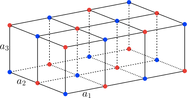
Figure 1: Optimal charge distribution for the orthorhombic lattice for $d=3$. The points in blue (resp. red) have charge $-1$ (resp. $1$).

We consider an ensemble of charges $\varphi_{x}$ located at the vertices $x\in X$ of a given $d$-dimensional Bravais lattice $X\subset\mathbb{R}^{d}$. For technical reasons, we also assume that the charges are $N$-periodic in each principal lattice direction for some $N\in\mathbb{N}$ and can be represented by the finite sublattice $K_{N}$ (for the precise definitions, we refer to the next section). The total interaction energy per lattice point can then be written as

$${\mathcal{E}}_{X,f}[\varphi]\ =\frac{1}{2N^{d}}\sum_{y\in K_{N}}\sum_{x\in X\backslash\{0\}}\varphi_{y}\varphi_{x+y}f(x),$$ (1.1)

for some radially symmetric interaction potential $f:\mathbb{R}^{d}\to[0,\infty)$. In the case, when $f$ is not absolutely summable on $X\backslash\{0\}$, the classic method of Ewald summation [32] is used to give a meaning to the infinite sum in (1.1). The class of interaction potentials $f$ we consider in particular includes all potentials $f(x)=F(|x|^{2})$ for some completely monotone function $F$. In particular, this includes all Riesz potentials of the form $f(x)=|x|^{-s}$ for some $s>0$. We consider the minimization problem

$$\varphi\mapsto{\mathcal{E}}_{X,f}[\varphi]$$

for all periodic charge configurations satisfying a constraint for the total charge (see (2.1)) and for any given Bravais lattice $X\subset\mathbb{R}^{d}$.

In our first result, we show that this minimization problem is related to a minimization of the translated lattice theta function

$$z\mapsto\theta_{X^{*}+z}(\alpha)=\sum_{p\in X^{*}}e^{-\pi\alpha|p+z|^{2}},$$ (1.2)

associated to the dual lattice $X^{*}$ in terms of the variable $z\in\mathbb{R}^{d}$ for given $\alpha>0$ (see Theorem 2.1). At the core of our proof lies an argument, originally due to Montgomery [44] and generalized by one of the authors in [11]. Theorem 2.1 can be used to calculate the optimal charge distribution in specific Bravais lattices if the minimization problem for the translated lattice theta function can be solved for these lattices. We first consider the situation of a $d$-dimensional orthorhombic lattice. In this case, the minimizer $z$ of (1.2) is the center of the primitive cell (for any $\alpha$) [11]. For the triangular lattice case, the minimizers are the two barycenters of the primitive triangles forming the primitive rhombic cell [6]. In both case, the knowledge of these minimizers gives us the minimal configuration of charges, that are the alternate rock salt configuration in the orthorhombic case (Theorem 2.4), see Fig. 1, and the honeycomb distribution for the triangular lattice (Theorem 2.6), see Fig. 2. In particular, Theorem 2.4 gives an affirmative answer to Born’s conjecture, cited above. Let us note that, in the case of Riesz potentials which are not summable over the lattice, also the analytic continuation of Epstein’s zeta function has been used to describe the lattice energies in this case, see e.g. [29]. Indeed, this approach yields the same energy as the Ewald method used in our approach.

We note that the translated lattice theta function appears in several mathematical models for physical systems with different kind of particles. For example, Ho and Mueller [45] wrote the interaction between two Bose-Einstein condensates in terms of translated lattice theta functions, and the same is done by Trizac et al. [53, 3] in the context of Wigner bilayers. Mathematically, the problem of minimizing $z\mapsto\theta_{X+z}(\alpha)$ was studied by Baernstein in [6] for $X=\Lambda_{1}$ a two-dimensional triangular lattice and by the first author in [11] for more general lattices.

Let us also recall related work for optimal lattice configurations for systems with the same kind of particles. The studies of lattice theta functions and Epstein zeta functions are originally due to Krazer and Prym [39] and Epstein [31]. Later, the problem of minimizing the Epstein zeta function among two-dimensional Bravais lattices with a fixed density was studied by Rankin [51], Ennola [30], Cassels [19] and Diananda [27] (see also the recent review [38]). They proved the optimality of the triangular lattice (also called Abrikosov lattice in the context of superconductivity). Montgomery [44] proved the optimality of the triangular lattice, among Bravais lattices with a fixed density, for the lattice theta function $X\mapsto\theta_{X}(\alpha)$, see also [46, Appendix A.2.]. This result and its consequence [20] has been used to show that the triangular configuration is a ground state of total interaction energy for a class of interaction potentials. Let us cite the works of Sandier and Serfaty [54] on Coulomb gases and superconductivity and their consequences for the logarithmic energy on the $2$-sphere in [12], but also the work of Aftalion, Blanc and Nier [1] on Bose-Einstein Condensates and that of Nonnenmacher-Voros [46] on chaotic maps over a torus phase space. Furthermore, Montgomery’s result was used by the first author and Zhang in [13, 8] in order to prove the optimality of the triangular lattice at high density for more general interaction energies. Furthermore, the authors also used this result in order to prove the optimality of the triangular lattice for radially symmetric, spatially extended particles interacting via a radial potential in [10]. In dimensions three, as recalled in [14, Section 2.5], the proof of the Sarnak-Strömbergsson conjecture [55] about the optimality, for the lattice theta function, of the Body-Centered-Cubic (resp. Face-Centered-Cubic) lattice at high (resp. low) density , would be an important advance both in analytic number theory and in solid-state physics, see also [52]. Some recent advances have been made by the first author in [11, 9], using recent results about Jacobi theta functions in [33]. In higher dimensions, the local minimality of some lattices for the lattice theta function, the Epstein zeta function and other related lattice energies was studied by Coulangeon et al. in [22, 24, 23, 25]. The above investigation are made under the assumption that the configuration can be expressed as a Bravais lattice. In a different approach without periodicity assumptions optimal lattice configurations have been studied e.g. in [59, 60, 37, 50, 58, 34, 28, 42, 43, 41].

The optimality of the alternate configuration (also called “chessboard configuration”) in a different setting is also discussed in [18]. Considering a flat torus ${\mathcal{T}}$ of a certain specific size, composed by $N\in 2\mathbb{N}$ points, associated with an orthorhombic lattice, the authors ask the following question: How can $N/2$ points on this grid be located such that the associated energy $E=\sum_{p\neq q\in{\mathcal{T}}}f(\delta(p,q))$ is minimized? Here, $f$ is a radial function and $\delta$ is the Lee distance, a graph distance counting the minimal number of edges of the grid connecting $p$ to $q$. Then, relaxing the problem by minimizing $\tilde{E}=\sum_{p\neq q\in{\mathcal{T}}}f(\delta(p,q))w(p)w(q)$, where $w(p)$ is a weight (corresponding to our charges), and translating this problem in Fourier space, they prove their result for a specific choice of $f$ (including completely monotone functions) and ${\mathcal{T}}$. It should be noted that there are some important difference in terms of the result and model in [18] with respect to this paper, even though the strategy of the proof is similar. One difference is that the results in [18] are concerned with finite sums in contrast to the infinite number of (long range) interactions energies considered in this work. Another difference is the graph distance considered in [18] which requires combinatorically arguments. In particular, they numerically show (see [18, Sect. 6.2]) that the Lee distance cannot be replaced by the Euclidean distance for their result involving completely monotone functions. On the other hand, it doesn’t seem to be straightforward to use our arguments to derive the results of [18]. We also note that the results in this paper apply to any lattice for which the minimizer of the translated theta function is known.

Structure of the paper: In the remaining parts of the first section, we introduce the mathematical formulation for the model, introduce some needed special functions and present useful identities for those. In Section 2, we state our main results in Theorems 2.1–2.7. The proofs of these theorems are given in Section 3.

Notation: We will write $(e_{i})_{1\leq i\leq d}$ for the canonical basis of $\mathbb{R}^{d}$. For any $x,y\in\mathbb{R}^{d}$, we denote the Euclidean scalar product by $x\cdot y$. We also use the notation $\llbracket a,b\rrbracket:=[a,b]\cap\mathbb{Z}$.

We recall that a Bravais lattice in $\mathbb{R}^{d}$ is a set points of the form $X=\bigoplus_{i=1}^{d}\mathbb{Z}u_{i}\subset\mathbb{R}^{d}$ for a given set of linearly independent vectors $u_{i}\in\mathbb{R}^{d}$ with $i\in\llbracket 1,d\rrbracket$. We call $A_{X}$ the generator matrix of the lattice $X$, i.e. $A_{X}\mathbb{Z}^{d}=X$. The associated quadratic form assigned with the Bravais lattice is given by $q_{X}(n)=\|\sum_{i=1}^{d}n_{i}u_{i}\|^{2}$ for $n\in\mathbb{Z}^{d}$. The dual lattice $X^{*}$ of the lattice $X$ is given by

$$X^{*}=\left\{p\in\mathbb{R}^{d}\ :\ p\cdot x\in\mathbb{Z}\text{ for all $x\in X$}\right\}.$$

1.2 The model

We consider configurations of charges located on the sites of $d$-dimensional Bravais lattices $X\in\mathbb{R}^{d}$ for any $d\geq 1$. We will assume without loss of generality that all considered Bravais lattices have unit density, i.e. the unit cell $Q:=\sum_{i=1}^{d}[0,1)u_{i}$ of the lattice has unit volume. The general case can be recovered by rescaling the lattice.

We consider charged lattices, where a charge is assigned to every lattice point:

Definition 1.1 (Charged lattice).

Let $d\geq 1$.

1. A charged lattice $L=(X,\varphi)$ is a Bravais lattice $X=\bigoplus_{i=1}^{d}\mathbb{Z}u_{i}$ together with a function $\varphi:X\to\mathbb{R}$ such that for any $x\in X$, the point $x$ has charge $\varphi_{x}=\varphi(x)$.

2. We say that the charge distribution is $N$-periodic if it is periodic with period $N$ in any coordinate direction, i.e.

   $$\varphi(x+Nu_{i})=\varphi(x) \text{for any $x\in X$ and any $i\in\llbracket 1,d\rrbracket$}.$$

   The charge distribution is called periodic if it is $N$-periodic for some $N\in\mathbb{N}$. We define the finite sublattice $K_{N}\subset X$ by

   $$K_{N}\ :=\ \Big{\{}x=\sum_{i=1}^{d}m_{i}u_{i}\in X\ :\ m_{i}\in\llbracket 0,N-1\rrbracket\text{ for all }i\in\llbracket 1,d\rrbracket\Big{\}},$$ (1.3)

   and we call $K_{N}^{*}$ the corresponding sublattice in $X^{*}$.

3. The space of $N$-periodic functions on the lattice is denoted by $\Lambda_{N}(X)$. It is equipped with inner product and norm by

   $$(\varphi,\psi)_{K_{N}}=\sum_{y\in K_{N}}\varphi(y)\overline{\psi(y)}, \|\varphi\|=\sqrt{(\varphi,\varphi)_{K_{N}}}\ .$$

Note that an $N$-periodic charge configuration is uniquely given by its values on the $N^{d}$ points on the finite sublattice $K_{N}$.

We will consider the following class of potentials:

Definition 1.2 (The class of interaction potentials).

For $d\geq 1$, we say that $f\in{\mathcal{F}}$ if $f:\mathbb{R}^{d}\to[0,+\infty)$ and if, for any $x\in\mathbb{R}^{d}\backslash\{0\}$, we have

$$f(x)=\int_{0}^{\infty}e^{-|x|^{2}t}d\mu_{f}(t),$$ (1.4)

where $\mu_{f}$ is a non-negative Borel measure. If $f$ is absolutely summable over $X\backslash\{0\}$, we use the notation $f\in\ell^{1}(X\backslash\{0\})$.

Note that the assumption in Definition 1.2 corresponds to the particular case of G-type potential defined in [35, Definition 1] where $\mu_{f}$ is non-negative.

Remark 1.3 (Relation to completely monotone functions).

The class ${\mathcal{F}}$ of admissible potentials is quite large. Indeed, by the Hausdorff-Bernstein-Widder theorem [7], (1.4) is equivalent to $f(x)=F(|x|^{2})$ for some completely monotone function $F:(0,\infty)\to\mathbb{R}$, i.e. for any $F$ which satisfies

$$(-1)^{k}F^{(k)}(r)\geq 0 \forall r>0,\forall k\in\mathbb{N}.$$

In particular, every potential of type

$$r^{-s},\ e^{-\lambda r^{\alpha}},\ \frac{e^{-\lambda r}}{r},\ \frac{e^{-\lambda\sqrt{r}}}{\sqrt{r}} \text{ for $s>0,$ $\lambda>0$, $\alpha\in(0,2]$},$$

is included in the class ${\mathcal{F}}$. Further examples can be constructed by noting that if $f,g$ are completely monotone, then $\alpha f+g$, $\alpha>0$ and $fg$ are completely monotone. On the other hand, the class of Lennard-Jones-type potentials of the form $V(r)=r^{-p}-br^{-q}$ with $b>0$ and $p>q$ are not included in ${\mathcal{F}}$.

Remark 1.4 (The logarithmic potential in $\mathbb{R}^{2}$).

In two dimensions, the Coulomb potential $f(x)=-\log|x|$ does not belong to ${\mathcal{F}}$. However, we believe that the results in this paper should hold for this potential as well. Indeed, this should follow by an approximation argument together with the formula

$$-\log|x|=\frac{1}{2}\lim_{\varepsilon\to 0^{+}}\Big{(}\int_{\varepsilon}^{\infty}\frac{e^{-t|x|^{2}}}{t}dt+\gamma+\log\varepsilon\Big{)},$$

where $\gamma\approx 0.577$ is the Euler-Mascheroni constant.

We assume that the interaction energy between two points of charges $\varphi_{x}$, $\varphi_{y}$ at positions $x,y\in X$ is given by $\varphi_{x}\varphi_{y}f(x-y)$ for some rotationally symmetric interaction potential $f\in{\mathcal{F}}$. If $f$ is absolutely summable over $X\backslash\{0\}$, the total potential energy is obtained directly by summing the interaction energies for all points of the lattice. If $f$ is not summable, the method of Ewald summation [32] (introduced by Ewald in his 1912 doctoral thesis) can be used to still define the total energy of the system assuming that the total net charge is zero. More precisely, as Born did in [16] for the Coulomb potential, we use the classic Gaussian convergence factors method, as in [26, 47, 35]:

Definition 1.5 (Interaction energy).

Let $N\geq 2$ and $L=(X,\varphi)$ be a charged lattice with $N$-periodic charge distribution $\varphi$ and let $f\in{\mathcal{F}}$. If $f\not\in\ell^{1}(X\backslash\{0\})$, we assume the charge neutrality condition,

$$\sum_{y\in K_{N}}\varphi_{y}=0.$$ (1.5)

The energy per particle is given by

$${\mathcal{E}}_{X,f}[\varphi]\ :=\lim_{\eta\to 0}\Big{(}\frac{1}{2N^{d}}\sum_{y\in K_{N}}\sum_{x\in X\backslash\{0\}}\varphi_{y}\varphi_{x+y}f(x)e^{-\eta|x|^{2}}\Big{)}.$$ (1.6)

We note that there are a variety of different ways to define the lattice energy for non-integrable interaction potentials (see e.g. [17]). The method of Ewald summation is commonly used to calculate the energy for different charged systems and has been optimized for computational speed, see e.g. [26, 49, 47]. We also note that the Ewald summation can also be used to calculate an energy for the case of non-neutral charge configurations [47, 2]. If the interaction potential is given by a non-integrable Riesz potential, i.e. $f(x)=|x|^{-s}$ for $s\in(0,d]$, then another way to define the energy is by analytic extension of the Epstein zeta function, introduced in [31]. We give the definition of the Epstein zeta function in slightly less generality as needed for our purposes.

Definition 1.6.

Let $X\subset\mathbb{R}^{d}$, $d\geq 1$, be a Bravais lattice associated with the positive definite quadratic form $q_{X}$. Then Epstein’s zeta function is defined by

$$\textnormal{Z}\left|\hskip-2.5pt\begin{array}[]{r}0\@arraycr z\end{array}\hskip-2.5pt\right|(q_{X};s):=\sum_{n\in\mathbb{Z}^{d}\backslash\{0\}}\frac{e^{2i\pi n\cdot z}}{[q_{X}(n)]^{\frac{s}{2}}} z\in\mathbb{R}^{d} s\in\{\mathbb{C}:\mathfrak{Re}s>d\}.$$ for ,

This function admits an analytic continuation beyond its domain of absolute convergence. For $s\in\mathbb{C}$ with $\mathfrak{Re}s>0$ and $z\not\in X^{*}$, the extension is given by

$$\pi^{-\frac{s}{2}}\Gamma(\frac{s}{2})\textnormal{Z}\left|\hskip-2.5pt\begin{array}[]{r}0\@arraycr z\end{array}\hskip-2.5pt\right|(q_{X};s)$$ (1.8)

$$\qquad=-\frac{2}{s}+\int_{1}^{\infty}\sum_{n\in\mathbb{Z}^{d}\backslash\{0\}}e^{2i\pi n\cdot z}e^{-\pi tq_{X}(n)}t^{\frac{s}{2}-1}dt+\int_{1}^{\infty}\sum_{n\in\mathbb{Z}^{d}}e^{-\pi tq_{X^{*}}(n+z)}t^{\frac{d-s}{2}-1}dt,$$

where $q_{X^{*}}$ is the quadratic form associated with the dual lattice $X^{*}$, see [31].

1.3 Discrete Fourier transform and convolution

The proofs are formulated in terms of the discrete Fourier transform (for an introduction, see e.g. [5, Chapter 6]) on the space of $N$-periodic functions $\Lambda_{N}(X)$ on the lattice $X$. We first note that an orthonormal basis of $\Lambda_{N}(X)$ is given by the functions , we define the functions by the functions $e^{(k)}\in\Lambda_{N}(X)$ where

$$e^{(k)}(y)=\frac{1}{N^{\frac{d}{2}}}e^{\frac{2\pi i}{N}y\cdot k}.$$

The discrete Fourier transform is then defined as follows:

Definition 1.7 (Discrete Fourier transform).

For any $\varphi\in\Lambda_{N}(X)$, its discrete Fourier transform $\widehat{\varphi}\in\Lambda_{N}(X^{*})$ is given by

$$\widehat{\varphi}(k)=(\varphi,e^{(k)})_{K_{N}} \text{for $k\in X^{*}$}.$$

where $e^{(k)}(y):=\frac{1}{N^{\frac{d}{2}}}e^{\frac{2\pi i}{N}y\cdot k}$. For $\psi\in\Lambda_{N}(X^{*})$, the inverse Fourier transform is

$$\savestack{\tmpbox}{\stretchto{\scaleto{\scalerel*[\widthof{\psi}]{\kern-0.6pt\bigwedge\kern-0.6pt}{\rule[-505.89pt]{4.30554pt}{505.89pt}}}{}}{0.5ex}}\stackon[1pt]{\psi}{\scalebox{-1.0}{\tmpbox}}(x)=(\psi,\overline{e^{(x)}})_{K_{N}^{*}} \text{for $x\in X$}.$$

Since the functions $e^{(k)}$ form an orthonormal basis, the Fourier transform is a bijective map $\Lambda_{N}(X)\to\Lambda_{N}(X^{*})$ whose inverse is given by the inverse Fourier transform. Furthermore, Plancherel’s identity holds with constant $1$, i.e.

$$(\varphi,\varphi)_{K_{N}}=(\widehat{\varphi},\widehat{\varphi})_{K_{N}^{*}},$$

since the discrete Fourier transform corresponds to the application of a unitary matrix. A simple calculation shows that $\widehat{\varphi*\psi}(k)=\widehat{\varphi}(k)\widehat{\psi}(k)$ for any $k\in X^{*}$, where the convolution is defined by

$$(\varphi*\psi)(p)=\sum_{q\in K_{N}}\varphi_{q}\psi_{p-q}.$$

1.4 Theta functions and useful identities

Theta functions play an important role in different fields of mathematics. For the computation of lattice sums, the following Jacobi theta function is useful:

Definition 1.8 (Jacobi Theta functions).

The third Jacobi theta function is defined by

$$\vartheta_{3}(\xi;z):=\sum_{k\in\mathbb{Z}}e^{i\pi k^{2}z+2i\pi k\xi},\quad\Im(z)>0,\xi\in\mathbb{C}.$$ (1.9)

We recall some useful identities for the Jacobi theta function restricted to the upper imaginary axis. This restriction has been considered by Montgomery in [44] (he wrote $\theta(t,\beta):=\vartheta_{3}(\beta,it)$) in the context of lattice sums:

Lemma 1.9.

Let $t>0$ and let $\beta\in\mathbb{R}$. Then

1. $\displaystyle\vartheta_{3}(\beta;it)=\prod_{r=1}^{\infty}\left(1-e^{-2\pi rt}\right)\left(1+2e^{-(2r-1)\pi t}\cos(2\pi\beta)+e^{-2(2r-1)\pi t}\right).$

2. $\displaystyle\vartheta_{3}(\beta;it)>0$.

3. The map $\beta\mapsto\vartheta_{3}(\beta;it)$ is $1$-periodic. Furthermore, we have

   $$\vartheta_{3}\Big{(}\frac{1}{2}-\beta;it\Big{)}=\vartheta_{3}\Big{(}\frac{1}{2}+\beta;it\Big{)} \beta\in[0,\tfrac{1}{2}]$$ for any . (1.10)

Proof.

The product formula (i) is proved for example in [57, Chapter 10, Theorem 1.3]. The positivity of $\vartheta_{3}$ follows by expressing the right hand side in the Jacobi product representation (i) of the theta function as

$$\vartheta_{3}(\beta;it)=\prod_{r=1}^{\infty}\big{(}1-e^{-2\pi rt}\big{)}\big{(}\sin^{2}(2\pi\beta))+\big{[}e^{-(2r-1)\pi t}+\cos(2\pi\beta)\big{]}^{2}\big{)}>0.$$

The periodicity is a direct consequence of formula (1.9). The statement (1.10) finally follows from (1.9) with the change of variables $q=-k$. ∎

Finally, we introduce the translated lattice theta function (see e.g. [21, Section 2.3]) which is a particular case of generalized lattice theta functions that have been studied by Krazer and Prym in [39]:

Definition 1.10 (Translated lattice theta function).

Let $d\geq 1$ and let $X=\bigoplus_{i=1}^{d}\mathbb{Z}u_{i}\subset\mathbb{R}^{d}$ be a Bravais lattice. Then the theta function of the translated lattice $X+z$ or translated lattice theta function is defined by

$$\theta_{X+z}(\alpha)\ :=\ \sum_{x\in X}e^{-\pi\alpha|x+z|^{2}} \alpha>0 z\in\mathbb{R}^{d}$$ for any .

The function $\theta_{X+z}(\alpha)$ can be understood as follows: Consider a matrix of points at the lattice points of $X$, carrying a unit charge. Suppose that the charges induce an interaction potential $\exp(-\pi\alpha|x|^{2})$. Then $\theta_{X+z}(\alpha)$ describes the (Gaussian) interaction energy between $z$ and $X$.

Remark 1.11 (Translated lattice theta function and heat flow).

An interpretation of $\theta_{X+z}$ in terms of the heat flow is given by Baernstein in [6]. Let $P_{X}$ be the temperature at point $z$ and at time $t$, if at time $t=0$ a heat source of unit strength is placed at each point of $X$, i.e. $P_{X}$ is defined, for any $z\in\mathbb{R}^{d}$, any Bravais lattice $X\subset\mathbb{R}^{d}$ and any $t>0$ as the solution of

$$\left\{\begin{array}[]{ll}\partial_{t}P_{X}(z,t)=\Delta_{z}P_{X}&\text{for $(z,t)\in\mathbb{R}^{d}\times(0,\infty)$}\vspace{0.3ex}\\ P_{X}(z,0)=\sum_{p\in X}\delta_{p}&\text{for $z\in\mathbb{R}^{d}$},\end{array}\right.$$

where $\delta_{p}$ is the Dirac measure at $p\in\mathbb{R}^{d}$. Then

$$\theta_{X+z}(\alpha)=\frac{1}{\alpha^{\frac{d}{2}}}P_{X}\left(z,\frac{1}{4\pi\alpha}\right) z\in\mathbb{R}^{d} \alpha>0$$ for , .

We next recall some basic facts related to the translated lattice theta function, introduced in Definition 1.10. We first recall Jacobi’s Transformation Formula:

Proposition 1.12 (Jacobi’s Transformation Formula).

For any Bravais lattice $X\subset\mathbb{R}^{d}$ of density one, any $\alpha>0$ and any $z\in\mathbb{R}^{d}$, we have

$$\theta_{X+z}(\alpha)=\sum_{x\in X}e^{-\alpha\pi|x+z|^{2}}=\frac{1}{\alpha^{\frac{d}{2}}}\sum_{p\in X^{*}}e^{2\pi ip\cdot z}e^{-\frac{\pi|p|^{2}}{\alpha}}.$$ (1.11)

Proof.

A proof (based on Poisson’s summation formula) can be found e.g. in [35, Theorem A]. See also [15] for a proof of a more general formula. ∎

For one-dimensional lattices the translated lattice theta function can be expressed in terms of Jacobi theta function. Furthermore, we state other useful identities related to scaling and periodicity of the translated lattice theta function:

Lemma 1.13.

Let $d\geq 1$ and let $X\subset\mathbb{R}^{d}$ be a Bravais lattice. Let $\alpha>0,\beta\in\mathbb{R}$, $z\in\mathbb{R}^{d}$ and let $\lambda\neq 0$. Then

1. $\displaystyle\theta_{\mathbb{Z}+\beta}(\alpha)=\frac{1}{\sqrt{\alpha}}\vartheta_{3}(\beta;i\alpha^{-1})$  for $X=\mathbb{Z}$.

2. $\displaystyle\theta_{\lambda X+z}(\alpha)=\theta_{X+\frac{z}{\lambda}}(\alpha\lambda^{2})$,

3. the map $z\mapsto\theta_{X+z}(\alpha)$ is periodic w.r.t. the unit cell $Q=\sum_{i=1}^{d}[0,1)u_{i}$.

Proof.

In terms of $t:=\frac{1}{\alpha}$, identity (i) is equivalent to

$$\vartheta_{3}(\beta;it)=\frac{1}{\sqrt{t}}\sum_{n\in\mathbb{Z}}e^{-\frac{\pi(n+\beta)^{2}}{t}}.$$ (1.12)

In turn (1.12) is a direct application of Jacobi’s transformation formula (1.11) for $X=\mathbb{Z}$. The identity (ii) is easily obtained by

$$\theta_{\lambda X+z}(\alpha)=\sum_{x\in X}e^{-\pi\alpha|\lambda x+z|^{2}}=\sum_{x\in X}e^{-\pi\alpha\lambda^{2}|x+\frac{z}{\lambda}|^{2}}=\theta_{X+\frac{z}{\lambda}}(\alpha\lambda^{2}).$$

Finally, the statement (iii) follows from the periodicity of $X$. ∎

Consequently, in view of (iii) for any fixed lattice $X$ and for given $\alpha>0$, the problem of minimizing $z\mapsto\theta_{X+z}(\alpha)$ can be restricted to $Q=\sum_{i=1}^{d}[0,1)u_{i}$.

Lemma 1.14 (Symmetry of the theta function).

Let $X=\bigoplus_{i=1}^{d}\mathbb{Z}u_{i}$ be a Bravais lattice and $T(z)=\sum_{i=1}^{d}u_{i}-z$ be the symmetry with respect to the center $c=\frac{1}{2}\sum_{i=1}^{d}u_{i}$ of the primitive cell $Q=\sum_{i=1}^{d}[0,1)u_{i}$. Then, for any $z\in\mathbb{R}^{d}$ and any $\alpha>0$, we have

$$\theta_{X+z}(\alpha)=\theta_{X+T(z)}(\alpha)$$

Proof.

We have, for any $z\in\mathbb{R}^{d}$ and any $\alpha>0$,

$$\theta_{X+T(z)}(\alpha)=\sum_{x\in X}e^{-\pi\alpha|x+T(z)|^{2}}=\sum_{x\in X}e^{-\pi\alpha|x+\sum_{i=1}^{d}u_{i}-z|^{2}}=\sum_{x\in X}e^{-\pi\alpha|x-z|^{2}}=\theta_{X+z}(\alpha),$$

by the periodicity of the translated theta function (Lemma 1.13(iii)) and the symmetry $-X=X$. ∎

2 Statement of main results

We consider minimizer of the interaction energy among periodic charge configurations. As in the paper by Born [16], we assume that the charges of the points of $K_{N}$ satisfy a constraint on the total charge per periodicity cell, i.e.

$$\frac{1}{N^{d}}\sum_{y\in K_{N}}\varphi_{y}^{2}\ =\ 1, \varphi(0)>0.$$ (2.1)

Our first result is a statement which connects the minimization of the energy for certain lattice energies with the minimization problem among vectors for the translated lattice theta function:

Theorem 2.1 (Optimal charge distributions and theta function).

Let $d\geq 1$, let $X=\bigoplus_{i=1}^{d}\mathbb{Z}u_{i}\subset\mathbb{R}^{d}$ be a Bravais lattice and let $f\in{\mathcal{F}}$. Suppose that

$$z_{0}\ \in\ \operatorname{argmin}\Big{\{}\theta_{X^{*}+z}(\alpha):z\in\sum_{i=1}^{d}\lambda_{i}u_{i}^{*}:\forall i,\lambda_{i}\in[0,1)\Big{\}} \forall\alpha>0,$$ (2.2)

i.e. $z_{0}$ is an absolute minimizer of the translated theta function associated to the dual lattice $X^{*}$ for all $\alpha>0$. Furthermore, suppose that $z_{0}\in\frac{1}{N}X^{*}$ for some $N\in\mathbb{N}$. Then the energy $\mathcal{E}_{X,f}$ is minimized among all periodic charge configurations $\varphi$ which satisfy (2.1) (and which satisfy (1.5) if $f$ is nonsummable) by

$$\varphi^{*}(x)=c\cos\left(2\pi x\cdot z_{0}\right) \text{for $x\in X$},$$ (2.3)

where the value of the constant $c$ is determined by (2.1).

Furthermore, if (2.2) has at most two solutions, then the charge configuration (2.3) is the unique minimizer of ${\mathcal{E}}_{X,f}$, up to symmetries keeping $X$ invariant. Otherwise, if (2.2) has more than two solutions then there are infinitely many minimizing charge configurations which are pairwise not related by symmetries keeping $X$ invariant.

We notice that $z_{0}$ defined by (2.2) is assumed to be a minimizer of $z\mapsto\theta_{X^{*}+z}(\alpha)$ for any $\alpha>0$. As we will see, that is the case if $X^{*}$ is an orthorhombic or triangular lattice, but it is not clear for which lattices this property remains true. In [11, Thm 1.5], it has been shown that a deep hole of $X$, i.e. a solution $c$ to $\max_{c\in\mathbb{R}^{d}}\min_{p\in X^{*}}|c-p|$ is an asymptotic minimizer for $z\mapsto\theta_{X^{*}+z}(\alpha)$ as $\alpha\to+\infty$. Furthermore, in [11, Thm 1.6], it has been proved that the asymptotic minimizers vary according to the structure of the lattice in dimension $2$, as it was also briefly explained in [6, p. 232]. Therefore, it appears that lattices $X$ with sufficient asymmetry do not have the same asymptotic minimizer for any $\alpha>0$. In dimension $2$, according to these results, rectangular and rhombic lattices (the two generating vectors of $X$ have the same length and the minimal interior angle of the unit cell belongs to $[\pi/3,\pi/2]$) as well as non-rhombic lattices such that the second layer (from the origin) of $X$ has cardinality $2$ or $6$ seem to be the good candidates for keeping the same minimizers for any $\alpha>0$. We are not aware of a proof of such property.

The explicit form of the minimizers in (2.3) implies in particular that the net charge for any minimizing configuration must be zero. We have the following corollary:

Corollary 2.2 (Charge neutrality).

Suppose that $f\in\ell^{1}(X\backslash\{0\})$. Then for any minimizer $\varphi^{*}$ of ${\mathcal{E}}_{X,f}$, the total net charge of the configuration is zero,

$$\sum_{y\in K_{N}}\varphi^{*}(y)=0.$$

We note that charge neutrality is assumed if $f$ is not absolutely summable. The corollary shows that charge neutrality also holds in the absolutely summable case.

Another interesting question is if there are lattices where there is no periodic optimal charge configuration. Here, Theorem 2.1 could be useful to prove such a non-existence result:

Remark 2.3 (Non-existence).

From the proof of Theorem 2.1, the following statement can be easily deduced: Let $d\geq 1$. Let $X=\bigoplus_{i=1}^{d}\mathbb{Z}u_{i}\subset\mathbb{R}^{d}$ be a Bravais lattice with dual lattice $X^{*}$. Suppose that $z_{0}$ is an absolute minimizer of the translated theta function for all $\alpha>0$, i.e. $z_{0}$ satisfies (2.2). Furthermore, suppose that

$$\operatorname{argmin}\Big{\{}\theta_{X^{*}+z}(\alpha):z\in\mathbb{R}^{d}\Big{\}}\cap\left\{\frac{1}{N}X^{*}:N\in\mathbb{N}\right\}=\emptyset.$$

Then the absolute minimum of the energy $\mathcal{E}_{X,f}$ is not obtained within the class of periodic charge configurations.

Together with a result obtained in [11, Cor. 3.17] about minimization of the translated lattice theta function for the orthorhombic lattice, we obtain the optimal charge distribution for orthorhombic (and in particular cubic) lattices. Indeed, for any orthorhombic lattice $X=\bigoplus_{i=1}^{d}\mathbb{Z}(b_{i}e_{i})\subset\mathbb{R}^{d}$, the unique minimizer of $z\mapsto\theta_{X+z}(\alpha)$ is, for any $\alpha>0$, the center of the unit cell $z_{0}=\frac{1}{2}\left(b_{1},...,b_{d}\right)$. We then get the following result:

Theorem 2.4 (Optimal charge distribution for orthorhombic lattices).

Let $d\geq 1$, let $f\in{\mathcal{F}}$ and let $X=\bigoplus_{i=1}^{d}\mathbb{Z}(a_{i}e_{i})\subset\mathbb{R}^{d}$ be an orthorhombic lattice with $a_{i}>0$ for $i\in\llbracket 1,d\rrbracket$. Then the minimizer $\varphi^{*}_{\rm orth}:X\to\mathbb{R}$ of ${\mathcal{E}}_{X,f}$ among all periodic charge distributions $\varphi:X\to\mathbb{R}$ satisfying the normalization constraint (2.1), and the charge neutrality constraint (1.5) if $f$ is nonsummable, is given by

$$\varphi^{*}_{\rm orth}\Big{(}\sum_{i=1}^{d}m_{i}a_{i}e_{i}\Big{)}=(-1)^{\sum_{i=1}^{d}m_{i}} \text{for all $m_{i}\in\mathbb{N}$, $i\in\llbracket 1,d\rrbracket$}.$$

The minimizer is unique up to translations by a vector in $X$.

Theorem 2.4 applies in particular for the case when $f$ is the Coulomb potential and $d=3$. Hence, Theorem 2.4 proves and generalizes Born’s conjecture about optimal charge distributions in [16] for cubic lattices and more general orthorhombic lattices. Moreover, we find again Born’s result [16, Section 4] in dimension $d=1$.

From the proof of Theorem 2.4, the following result for general lattices can be deduced:

Corollary 2.5 (The case of alternating charges).

Let $d\geq 1$, let $f\in{\mathcal{F}}$ and let $X=\bigoplus_{i=1}^{d}\mathbb{Z}u_{i}\subset\mathbb{R}^{d}$ be a Bravais lattice. Furthermore, suppose that the equation (2.2) only has a unique solution $z_{0}\in\sum_{i=1}^{d}[0,1)u_{i}^{*}$. Then the unique, up to translations by a vector of $X$, periodic charge configuration $\varphi$ which minimizes the energy ${\mathcal{E}}_{X,f}$ is the alternating configuration

$$\varphi^{*}_{\rm orth}\Big{(}\sum_{i=1}^{d}m_{i}u_{i}\Big{)}=(-1)^{\sum_{i=1}^{d}m_{i}} \text{for all $m_{i}\in\mathbb{N}$, $i\in\llbracket 1,d\rrbracket$}.$$

In the general case of arbitrary Bravais lattices, the minimizer of the translated lattice theta function $z\mapsto\theta_{X^{*}+z}(\alpha)$ is not known. However, in the special case of the triangular lattice in two dimensions, this theta function is well understood – its minimizers are the two barycenters of the primitive triangles – and we obtain the optimal solution for the charge distribution problem. Recall that the triangular lattice of unit density in two dimensions is given by the set

$$\Lambda_{1}=\mathbb{Z}u_{1}\oplus\mathbb{Z}u_{2}, u_{1}=\sqrt{\tfrac{2}{\sqrt{3}}}\left(\hskip-5.0pt\begin{array}[]{r}1\@arraycr 0\end{array}\hskip-5.0pt\right) u_{2}=\sqrt{\tfrac{2}{\sqrt{3}}}\left(\hskip-5.0pt\begin{array}[]{r}1/2\@arraycr\sqrt{3}/2\end{array}\hskip-5.0pt\right)$$ where ,   . (2.6)

The situation here is slightly different than in the orthorhombic case:

Theorem 2.6 (Optimal charge distribution for the triangular lattice).

Let $\Lambda_{1}\subset\mathbb{R}^{2}$ be the triangular lattice, defined in (2.6) and let $f\in{\mathcal{F}}$. Then the minimizer of ${\mathcal{E}}_{\Lambda_{1},f}$ among all periodic charge distributions $\varphi:\Lambda_{1}\to\mathbb{R}$ which satisfy the normalization constraint (2.1), and the charge neutrality constraint (1.5) if $f$ is nonsummable, is

$$\varphi^{*}_{\rm tri}(mu_{1}+nu_{2})=\sqrt{2}\cos\Big{(}\frac{2\pi}{3}(m+n)\Big{)} m,n\in\mathbb{Z}$$ for .

This minimizer is unique, up translations and rotations which keep $\Lambda$ invariant.

We note that by definition the lattice points of the triangular lattice are $1$-periodic. The charges are, however, not periodic with the same periodicity. Indeed, the minimizer $\varphi^{*}_{\rm tri}$ is $3$-periodic. The optimal charge distribution for the triangular lattice is sketched in Figure 2. One can think of the lattice as being realized by two different types of particles. The first (depicted in red) carries the charge $\sqrt{2}$, while the other type particle (depicted in blue) carries the charge $-\sqrt{2}/2$. Since there are twice as many particles of the second type than of the first type, the configuration is charge neutral.

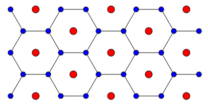
Figure 2: Optimal configuration $\varphi^{*}_{\rm tri}$ in the case of triangular lattice

This honeycomb structure with two kind of particles given by Figure 2 appears in different simulations and experiments. In [4], this structure arises as the minimizer of a binary mixture of particles interacting via the pair potential $V(r)=r^{-3}$ (up to a multiplicative constant) of parallel dipoles, at zero temperature, when the ratio of type particles is $(1/3,2/3)$ and at weak dipole-strength asymmetry. This result explains the experimental finding of [36, Figure 5.(a)]. Furthermore, the triangular lattice with the same absolute values of charges (i.e. $\sqrt{2}$ and $\sqrt{2}/2$) as in Theorem 2.6 is numerically identified in [61, 40] as a minimizer of the Coulomb interaction energy when the particles, with positive charges, are fixed on a triangular lattice embedded in a negative background charge to ensure neutrality. However, contrary to our study, these works investigated the minimizer of the interaction energy when the charges are fixed and as the concentrations (or the dipole-strength asymmetry) of the species vary.

Let us note that the method of Ewald summation in our case yields the same formula for the energy (up to an $s$ dependent constant) as the one obtained by analytic extension of Epstein’s zeta function:

Theorem 2.7 (Relation to Epstein’s Zeta function).

Let $d\geq 1$, $N\geq 2$, $X\subset\mathbb{R}^{d}$ be a Bravais lattice with generator matrix $A_{X}$, and $f_{s}(x)=|x|^{-s}$, $0<s\leq d$. For any $\varphi$ satisfying (2.1) and (1.5), for the $(\xi_{k})_{k\in K_{N}^{*}}$ defined in (3.3), we have $\xi_{k}\geq 0$ for any $k$ and

$${\mathcal{E}}_{X,f_{s}}[\varphi]=\frac{1}{2N^{d}}\sum_{k\in K_{N}^{*}}\xi_{k}\textnormal{Z}\left|\hskip-2.5pt\begin{array}[]{r}0\@arraycr A_{X}^{t}\frac{k}{N}\end{array}\hskip-2.5pt\right|(q_{X};s).$$

3 Proofs

3.1 Proof of Theorem 2.1 and Corollary 2.2

We first give the proof of the Theorem in the case when the interaction potential is absolutely summable over $X\backslash\{0\}$. We then will extend the result to the case when the interaction potential is not absolutely summable.

The absolutely summable case.

In the first part of the proof (Lemma 3.1–3.3), we follow the lines of the proof of Born in a slightly more general setting to write the energy in terms of the Fourier series [16], see Lemma 3.2. In the notation of Born, the corresponding plane waves $e^{\frac{2i\pi}{N}x\cdot k}$ are called “Grundpotentiale”. In the second step, we write the transformed expression of the energy in terms of the translated lattice theta functions $\theta_{X^{*}+\frac{k}{N}}(\alpha)$.

We first note express the energy in terms of the autocorrelation function $s$:

Lemma 3.1 (Energy expressed in $s$).

Let $d\geq 1$ and let $X\subset\mathbb{R}^{d}$ be a Bravais lattice. Let $N\geq 2$ and let $\varphi:X\to\mathbb{R}$ be an $N$-periodic charge distribution satisfying (2.1). Let $s:X\to\mathbb{R}$ be defined by

$$s_{x}:=\sum_{y\in K_{N}}\varphi_{y}\varphi_{y+x}.$$ (3.1)

Then $s\in\Lambda_{N}(X)$, $s_{-x}=s_{x}$, $\displaystyle\sum_{x\in K_{N}}s_{x}=\Big{(}\sum_{x\in K_{N}}\varphi_{x}\Big{)}^{2}$ and $s(0)=N^{d}$. The energy takes the form

$${\mathcal{E}}_{X,f}[\varphi]\ \stackrel{{\scriptstyle\eqref{ene}}}{{=}}\frac{1}{2N^{d}}\sum_{x\in X\backslash\{0\}}s_{x}f(x).$$ (3.2)

Proof.

The formula (3.2) follows directly from the definition of energy

$${\mathcal{E}}_{X,f}[\varphi]\ \stackrel{{\scriptstyle\eqref{ene}}}{{=}}\frac{1}{2N^{d}}\sum_{y\in K_{N}}\sum_{x\in X\backslash\{0\}}\varphi_{y}\varphi_{y+x}f(x).$$

by exchanging the sums. The periodicity of $\varphi$ implies $s_{-x}=s_{x}$ for any $x\in X$. One can easily check that $s(0)=\|\varphi\|_{K_{N}}^{2}=N^{d}$. Furthermore, by periodicity of $\varphi$, we obtain

$$\sum_{x\in K_{N}}s_{x}=\sum_{x\in K_{N}}\sum_{y\in K_{N}}\varphi_{y}\varphi_{y+x}=\sum_{y\in K_{N}}\varphi_{y}\sum_{x\in K_{N}}\varphi_{x+y}=\Big{(}\sum_{x\in K_{N}}\varphi_{x}\Big{)}^{2}.$$

∎

It is convenient to express the energy in terms of the discrete (inverse) Fourier transform $\xi$ of the autocorrelation function $s$. In the context of signal processing, $\xi$ has also been called energy spectral density.

Lemma 3.2 (Energy expressed in dual variables).

Let $d\geq 1$ and let $X\subset\mathbb{R}^{d}$ be a Bravais lattice. For $N\geq 2$, let $\varphi\in\Lambda_{N}(X)$ satisfy (2.1) and let $s$ be defined as in (3.1). Let $\xi\in\Lambda_{N}(X^{*})$ be given by

$$\xi_{k}:=\frac{1}{N^{d}}\sum_{y\in K_{N}}s_{y}e^{\frac{2\pi i}{N}y\cdot k} k\in X^{*}$$ for . (3.3)

Then $\xi_{k}\in\mathbb{R}$, $\xi_{k}\geq 0$, $\displaystyle\xi_{0}=\frac{1}{N^{d}}\Big{(}\sum_{x\in K_{N}}\varphi_{x}\Big{)}^{2}$ and $\xi_{k}=\xi_{-k}$ for all $k\in X^{*}$, and

$$\frac{1}{N^{d}}\sum_{k\in K_{N}^{*}}\xi_{k}=1.$$ (3.4)

Furthermore, the energy $E_{X,f}[\varphi]$ can be equivalently written as

$${\mathcal{E}}_{X,f}[\varphi]=\frac{1}{2N^{d}}\sum_{k\in K_{N}^{*}}\xi_{k}\sum_{x\in X\backslash\{0\}}e^{\frac{2\pi i}{N}x\cdot k}f(x).$$ (3.5)

Proof.

Note that $\xi=N^{-\frac{d}{2}}\savestack{\tmpbox}{\stretchto{\scaleto{\scalerel*[\widthof{s}]{\kern-0.6pt\bigwedge\kern-0.6pt}{\rule[-505.89pt]{4.30554pt}{505.89pt}}}{}}{0.5ex}}\stackon[1pt]{s}{\scalebox{-1.0}{\tmpbox}}$. Since $s_{-x}=s_{x}$ for any $x\in X$, we have $\xi\in\mathbb{R}$. The proof is based on Plancherel’s identity on $\Lambda_{N}(X)$. We give the calculation in detail below, using for notational simplicity, the convention $f(0):=0$. We have, using the symmetry $f(-q)=f(q)$,

$$\sum_{x\in X\backslash\{0\}}s_{x}f(x) =\sum_{\ell\in X}\sum_{y\in K_{N}}s_{y}f(N\ell+y)=\sum_{\ell\in X}\sum_{y\in K_{N}}\Big{(}\sum_{k\in K_{N}^{*}}\xi_{k}e^{\frac{-2\pi i}{N}y\cdot k}\Big{)}f(N\ell+y)$$

$$=\sum_{k\in K_{N}^{*}}\xi_{k}\sum_{x\in X\backslash\{0\}}e^{\frac{2\pi i}{N}x\cdot k}f(x).$$

Furthermore, $\xi=N^{-\frac{d}{2}}\savestack{\tmpbox}{\stretchto{\scaleto{\scalerel*[\widthof{s}]{\kern-0.6pt\bigwedge\kern-0.6pt}{\rule[-505.89pt]{4.30554pt}{505.89pt}}}{}}{0.5ex}}\stackon[1pt]{s}{\scalebox{-1.0}{\tmpbox}}=N^{-\frac{d}{2}}\savestack{\tmpbox}{\stretchto{\scaleto{\scalerel*[\widthof{\varphi*(\varphi\circ P)}]{\kern-0.6pt\bigwedge\kern-0.6pt}{\rule[-505.89pt]{4.30554pt}{505.89pt}}}{}}{0.5ex}}\stackon[1pt]{\varphi*(\varphi\circ P)}{\scalebox{-1.0}{\tmpbox}}=|\savestack{\tmpbox}{\stretchto{\scaleto{\scalerel*[\widthof{\varphi}]{\kern-0.6pt\bigwedge\kern-0.6pt}{\rule[-505.89pt]{4.30554pt}{505.89pt}}}{}}{0.5ex}}\stackon[1pt]{\varphi}{\scalebox{-1.0}{\tmpbox}}|^{2}\geq 0$, where $P(x)=-x$. The value of $\xi_{0}$ follows from $\sum_{x\in K_{N}}s_{x}=\left(\sum_{x\in K_{N}}\varphi_{x}\right)^{2}$ (see Lemma 3.1). Finally, one can easily check that $(\xi,1)_{K_{N}^{*}}=s(0)=N^{d}$. ∎

Note that due to the inversion symmetry of $s_{x}$ and $f(x)$, the sums on the right hand side of (3.3) and (3.5) are real numbers. By combining the sums over positive and negative indices, (3.5) can e.g. be written as

$${\mathcal{E}}_{X,f}[\varphi]=\frac{1}{2N^{d}}\sum_{k\in K_{N}^{*}}\xi_{k}\sum_{x\in X\backslash\{0\}}\cos\Big{(}\frac{2\pi}{N}x\cdot k\Big{)}f(x).$$

We also have the reverse transformation. Note that for given $\xi$, $\varphi$ is not uniquely defined in general.

Lemma 3.3.

Let $\xi\in\Lambda_{N}(X^{*})$ satisfy $\xi\geq 0$, $\xi_{-k}=\xi_{k}$ and (3.4). Let

$$\varphi_{x}=\frac{1}{N^{\frac{d}{2}}}\sum_{k\in K_{N}^{*}}\sqrt{\xi_{k}}\ \cos\Big{(}\frac{2\pi}{N}x\cdot k\Big{)}.$$ (3.6)

Then $\varphi$ satisfies (2.1) and the formulas (3.1) and (3.3) hold.

Proof.

We define $s\in\Lambda_{N}(X)$ by $s=N^{\frac{d}{2}}\widehat{\xi}$, i.e.

$$s_{x}=\sum_{k\in K_{N}^{*}}\xi_{k}e^{-\frac{2\pi i}{N}x\cdot k},$$

so that (3.3) holds. A straightforward calculation now shows that the identities (2.1) and (3.1) are satisfied by the function $\varphi$ defined in (3.6). ∎

We turn to the proof of Theorem in the case when the interaction potential is summable:

Proposition 3.4 (Theorem $1$ — the summable case).

Suppose that the assumptions of Theorem 2.1 hold and suppose that $f\in\ell^{1}(X\backslash\{0\})$. Then the statement of Theorem 2.1 holds

Proof.

Let $s$ and $\xi$ be defined as in Lemma 3.1 and Lemma 3.2. Then we have

$${\mathcal{E}}_{X,f}[\varphi]=\frac{1}{2N^{d}}\sum_{k\in K_{N}^{*}}\xi_{k}\sum_{x\in X\backslash\{0\}}e^{\frac{2\pi i}{N}x\cdot k}f(x).$$

where $\xi\geq 0$ and $\xi$ satisfies (3.4). This suggests to consider

$$E[k]\ :=\ \sum_{x\in X\backslash\{0\}}e^{\frac{2i\pi}{N}x\cdot k}f(x).$$ (3.7)

for $k\in X^{*}$. We note that $E[k]$ cannot be minimized for $k\in NX^{*}$. Indeed, in this case the energy decreases by just switching the sign of a single charge in the periodicity cell. In the following, we hence assume that $k\in X^{*}\backslash NX^{*}$.

In view of Definition 1.2 and by Fubini’s Theorem, we get for any $k\in X^{*}\backslash NX^{*}$,

$$E[k] =\sum_{x\in X\backslash\{0\}}\int_{0}^{\infty}e^{-|x|^{2}t}e^{2\pi ix\cdot\frac{k}{N}}d\mu_{f}(t)=\int_{0}^{\infty}\Big{(}\sum_{x\in X}e^{-|x|^{2}t}e^{2\pi ix\cdot\frac{k}{N}}-1\Big{)}d\mu_{f}(t).$$

By Jacobi’s transformation formula (1.11), this implies

$$E[k] =\int_{0}^{\infty}\Big{(}\pi^{\frac{d}{2}}t^{-\frac{d}{2}}\sum_{p\in X^{*}}e^{-\frac{\pi^{2}}{t}|p+\frac{k}{N}|^{2}}-1\Big{)}d\mu_{f}(t)$$

$$=\int_{0}^{\infty}\Big{(}\pi^{\frac{d}{2}}t^{-\frac{d}{2}}\theta_{X^{*}+\frac{k}{N}}(\tfrac{\pi}{t})-1\Big{)}d\mu_{f}(t).$$

Since $\mu_{f}$ is a non-negative measure, if $z_{0}$ is a minimizer on $X^{*}$ of $z\mapsto\theta_{X^{*}+z}(\alpha)$ for all $\alpha>0$, then $k_{0}=Nz_{0}$ minimizes $E$. By Lemma 3.3, a minimizing configuration $\varphi^{*}$ is then given, for any $x\in X$, by

$$\varphi^{*}(x)=c\cos\big{(}2\pi x\cdot z_{0}\big{)},$$ (3.8)

where $c$ is determined by the constraint (2.1). This concludes the proof of existence.

We turn to the proof of uniqueness. By assumption there are at most two minimizers $k_{0}$ and $k_{1}$ of $E[k]$. In view of Lemma 1.14, these two minimizers are symmetry related, i.e. we have $\frac{k_{1}}{N}=\sum_{i=1}^{d}u_{i}^{*}-\frac{k_{0}}{N}$. Therefore, the minimizer of (3.5) in the class of functions $\xi^{*}$ which satisfy $\xi^{*}\geq 0$, $\xi_{-k}^{*}=\xi_{k}^{*}$ for any $k\in X^{*}$ and (3.4) is hence given by $\xi^{*}\in\Lambda_{N}(X^{*})$, defined by $\xi_{k_{0}}^{*}=\xi_{k_{1}}^{*}=\frac{N^{d}}{2}$, by periodicity and the fact that $\xi_{k_{0}}^{*}=\xi_{-k_{0}}^{*}$, and $\xi_{k}^{*}=0$ for $k\in K_{N}^{*}\backslash\{k_{0},k_{1}\}$. It follows that the corresponding autocorrelation function $s^{*}$ is given, for any $x\in X$, by

$$s^{*}_{x}=\frac{N^{d}}{2}\left(e^{\frac{2i\pi}{N}k_{0}\cdot x}+e^{\frac{2i\pi}{N}k_{1}\cdot x}\right)=\frac{N^{d}}{2}\left(e^{\frac{2i\pi}{N}k_{0}\cdot x}+e^{-\frac{2i\pi}{N}k_{0}\cdot x}\right)$$ (3.9)

For any charge configuration $\varphi^{*}\in\Lambda_{N}(X)$, its (inverse) Fourier coefficients $\savestack{\tmpbox}{\stretchto{\scaleto{\scalerel*[\widthof{\varphi^{*}_{k}}]{\kern-0.6pt\bigwedge\kern-0.6pt}{\rule[-505.89pt]{4.30554pt}{505.89pt}}}{}}{0.5ex}}\stackon[1pt]{\varphi^{*}_{k}}{\scalebox{-1.0}{\tmpbox}}$ satisfy the equation $|\savestack{\tmpbox}{\stretchto{\scaleto{\scalerel*[\widthof{\varphi^{*}_{k}}]{\kern-0.6pt\bigwedge\kern-0.6pt}{\rule[-505.89pt]{4.30554pt}{505.89pt}}}{}}{0.5ex}}\stackon[1pt]{\varphi^{*}_{k}}{\scalebox{-1.0}{\tmpbox}}|^{2}=\xi_{k}^{*}$ as a straightforward calculation shows. Any charge configuration with associated autocorrelation function $s$, given by (3.9) therefore is of the form

$$\varphi^{*}_{x}=\frac{\alpha_{1}}{\sqrt{2}}e^{\frac{2i\pi}{N}k_{0}\cdot x}+\frac{\alpha_{2}}{\sqrt{2}}e^{-\frac{2i\pi}{N}k_{0}\cdot x}$$ (3.10)

for coefficients $\alpha_{i}\in\mathbb{C}$ with $|\alpha_{i}|=1$. We next use the fact that the charge configuration $\varphi^{*}$ is real. Furthermore, by a shift of coordinates, we can assume that $\varphi^{*}_{0}>0$ and that $\varphi^{*}$ attains its maximum at $x=0$. With these assumptions, one can show that $\alpha_{1}=1$ and $\alpha_{2}=1$. Therefore, in the case considered the charge distribution $\varphi^{*}$ is uniquely determined by the autocorrelation function $s$ and is hence unique and given by (3.8).

Suppose that there are at least three solutions of (2.2). Then as above we can construct two symmetric functions $\xi^{(1)},\xi^{(2)}\in\Lambda_{N}(X^{*})$ satisfying the properties of Lemma 3.2. Then any convex combination of $\xi^{(\theta)}:=\theta\xi^{(1)}+(1-\theta)\xi^{(2)}$ for $\theta\in[0,1]$ yields a minimizing charge configuration $\varphi^{(\theta)}$ (by Lemma 3.3). We hence have constructed a one-parameter family of optimal charge configurations $\varphi^{(\theta)}$ such that the corresponding autocorrelation functions $s_{\theta}$ are pairwise different. ∎

Proof of Corollary 2.2.

Let $\varphi^{*}\in\Lambda_{N}(X)$ be a minimizer of ${\mathcal{E}}_{X,f}$ and let $s^{*}$ and $\xi^{*}$ be defined by (3.1) and (3.3). In view of the proof of Theorem 2.1, it then follows that $\xi^{*}$ is the convex combinations of functions $\xi$ with $\xi_{0}=0$. It follows that $\xi^{*}_{0}=0$. In view of Lemma 3.2, this shows that the configuration is charge neutral. ∎

The nonsummable case

We turn to the case when the potential energy is not summable. In this case, the total energy of the lattice can be calculated using the Ewald summation method. The idea of Ewald summation with Gaussian convergent factor is to approximate the energy by replacing the interaction potential $f(x)$ by a family of screened interaction potentials $f(x)e^{-\eta|x|^{2}}$ (for some small parameter $\eta>0$), and to split the screened interaction potential into a short-range part and a long-range part (for some cut-off parameter $\alpha>0$). We follow the strategy in [47] where the Ewald summation has been used to calculate the energy of the Riesz potentials $f_{s}(x)=|x|^{-s}$ in dimensions $d=1,2,3$ and for $s\geq 1$ in a general setting without assuming charge neutrality.

Theorem 3.5 (Ewald summation).

Let $d\geq 1$, let $X\subset\mathbb{R}^{d}$ be a Bravais lattice and $f\in{\mathcal{F}}$. Then, for any $N\geq 2$, any $N$-periodic charge distribution $\varphi$ satisfying (2.1) and (1.5), and for any $\nu>0$, we have

$${\mathcal{E}}_{X,f}[\varphi] =\frac{1}{2N^{d}}\sum_{x\in X\backslash\{0\}}s_{x}f_{1}^{(\nu)}(x)+\frac{1}{2N^{d}}\sum_{p\in X^{*}}\xi_{p}f_{2}^{(\nu)}\left(\frac{{p}}{N}\right)-\frac{\mu_{f}\left([0,\nu^{2}]\right)}{2},$$

where

$$f_{1}^{(\nu)}(x)=\int_{\nu^{2}}^{+\infty}e^{-t|x|^{2}}d\mu_{f}(t), f_{2}^{(\nu)}(x)=\pi^{\frac{d}{2}}\int_{0}^{\nu^{2}}t^{-\frac{d}{2}}e^{-\frac{\pi^{2}}{t}|x|^{2}}d\mu_{f}(t).$$ (3.11)

Proof.

We write the approximated interaction potential as

$$f(x)e^{-\eta|x|^{2}}=\int_{0}^{\nu^{2}}e^{-(t+\eta)|x|^{2}}d\mu_{f}(t)+\int_{\nu^{2}}^{+\infty}e^{-(t+\eta)|x|^{2}}d\mu_{f}(t).$$ (3.12)

The second integral in (3.12) is absolutely integrable and the limit $\eta\to 0$ can be taken directly. We hence obtain

$${\mathcal{E}}_{X,f}[\varphi]\ =\lim_{\eta\to 0}\Big{(}\frac{1}{2N^{d}}\sum_{x\in X\backslash\{0\}}s_{x}f(x)e^{-\eta|x|^{2}}\Big{)}=\frac{1}{2N^{d}}\sum_{x\in X\backslash\{0\}}s_{x}f_{1}^{(\nu)}(x)+I_{2},$$

where

$$I_{2}:=\lim_{\eta\to 0}\Big{(}\frac{1}{2N^{d}}\sum_{x\in X\backslash\{0\}}s_{x}\int_{0}^{\nu^{2}}e^{-(t+\eta)|x|^{2}}\ d\mu_{f}(t)\Big{)}.$$

For the term $I_{2}$, we transform into dual variables with help of Jacobi’s transformation formula (1.11). Taking into account the fact that $s_{0}=N^{d}$, we have

$$\sum_{x\in X\backslash\{0\}}s_{x}e^{-(t+\eta)|x|^{2}} =\sum_{\ell\in X}\sum_{y\in K_{N}}s_{y}e^{-(t+\eta)|y+N\ell|^{2}}-N^{d}$$

$$=\frac{\pi^{\frac{d}{2}}}{(t+\eta)^{\frac{d}{2}}N^{d}}\sum_{y\in K_{N}}s_{y}\sum_{{p}\in X^{*}}e^{2\pi i{p}\cdot\frac{y}{N}}e^{-\frac{\pi^{2}}{(t+\eta)N^{2}}|{p}|^{2}}-N^{d}.$$

In view of the definition of $\xi$ in Lemma 3.2, we get

$$\sum_{x\in X\backslash\{0\}}s_{x}e^{-(t+\eta)|x|^{2}} =\frac{\pi^{\frac{d}{2}}}{(t+\eta)^{\frac{d}{2}}}\sum_{{p}\in X^{*}}\xi_{p}e^{-\frac{\pi^{2}}{(t+\eta)N^{2}}|{p}|^{2}}-N^{d}.$$

Hence, since $\xi_{0}=0$ as a consequence of the charge neutrality of $\varphi$, we arrive at

$$I_{2} =\frac{\pi^{\frac{d}{2}}}{2N^{d}}\lim_{\eta\to 0}\sum_{p\in X^{*}}\xi_{p}\int_{0}^{\nu^{2}}(t+\eta)^{-\frac{d}{2}}e^{-\frac{\pi^{2}}{(t+\eta)N^{2}}|p|^{2}}d\mu_{f}(t)-\frac{1}{2}\int_{0}^{\nu^{2}}d\mu_{f}(t)$$

$$=\frac{\pi^{\frac{d}{2}}}{2N^{d}}\sum_{p\in X^{*}}\xi_{p}\int_{0}^{\nu^{2}}t^{-\frac{d}{2}}e^{-\frac{\pi^{2}}{t}\left|\frac{p}{N}\right|^{2}}d\mu_{f}(t)-\frac{\mu_{f}\left([0,\nu^{2}]\right)}{2},$$

and the result is proved. ∎

Following the same arguments as in the summable case, we get

Lemma 3.6 (Energy expressed in dual variables).

Let $d\geq 1$, $X\subset\mathbb{R}^{d}$ be a Bravais lattice and $f\in{\mathcal{F}}$. Let $N\geq 2$ and let $\varphi:X\to\mathbb{R}$ be a $N$-periodic charge distribution satisfying (2.1). Let $s$ and $\xi$ be defined as in (3.1) and (3.3). Then $\xi$ is $N$-periodic and satisfies $\xi\in\mathbb{R}$, $\xi\geq 0$ and $\xi_{-k}=\xi_{k}$. The constraint (2.1) takes the form $(\xi,1)=N^{d}$ and the energy ${\mathcal{E}}_{X,f}[\varphi]$ is expressed as

$${\mathcal{E}}_{X,f}[\varphi]= \frac{1}{2N^{d}}\sum_{k\in K_{N}^{*}}\xi_{k}\Big{(}\sum_{x\in X\backslash\{0\}}e^{\frac{2\pi i}{N}x\cdot k}f_{1}^{(\nu)}(x)+\sum_{q\in X^{*}}f_{2}^{(\nu)}(q+\tfrac{k}{N})\Big{)}-\frac{\mu_{f}\left([0,\nu^{2}]\right)}{2}.$$

Proof.

The argument for both sums proceeds analogously as in the proof of Lemma 3.2, using the fact that $\xi_{0}=N^{-d}\sum_{p\in K_{N}}s_{p}=0$ because $\varphi$ satisfies (1.5). ∎

We are ready to give the proof of Theorem 2.1 in the non-summable case:

Proof of Theorem 2.1 in the non-summable case.

We have already shown that the statement of Theorem holds if $f$ is summable. We conclude the argument now for the non-summable case. By Lemma 3.6, we have

$${\mathcal{E}}_{X,f}[\varphi]= \frac{1}{2N^{d}}\sum_{k\in K_{N}^{*}}\xi_{k}\Big{(}\sum_{x\in X\backslash\{0\}}e^{\frac{2\pi i}{N}x\cdot k}f_{1}^{(\nu)}(x)+\sum_{q\in X^{*}}f_{2}^{(\nu)}(q+\tfrac{k}{N})\Big{)}-\frac{\mu_{f}\left([0,\nu^{2}]\right)}{2}.$$ (3.13)

Hence, it is enough to minimize

$$F[k] :=\sum_{x\in X\backslash\{0\}}e^{\frac{2\pi i}{N}x\cdot k}f_{1}^{(\nu)}(x)+\sum_{q\in X^{*}}f_{2}^{(\nu)}(q+\tfrac{k}{N})$$ (3.14)

$$=\int_{\nu^{2}}^{+\infty}\sum_{x\in X\backslash\{0\}}e^{\frac{2\pi i}{N}x\cdot k}e^{-t|x|^{2}}d\mu_{f}(t)++\pi^{\frac{d}{2}}\int_{0}^{\nu^{2}}\Big{(}\sum_{q\in X^{*}}e^{-\frac{\pi^{2}}{t}|q+\frac{k}{N}|^{2}}\Big{)}t^{-\frac{d}{2}}d\mu_{f}(t).$$

By application of Jacobi’s transformation formula (1.11), this implies

$$F[k] =\int_{\nu^{2}}^{\infty}\Big{(}\frac{\pi^{\frac{d}{2}}}{t^{\frac{d}{2}}}\sum_{p\in X^{*}}e^{-\frac{\pi^{2}}{t}|p+\frac{k}{N}|^{2}}-1\Big{)}d\mu_{f}(t)$$

$$\qquad+\pi^{\frac{d}{2}}\int_{0}^{\nu^{2}}\Big{(}\sum_{q\in X^{*}}e^{-\frac{\pi^{2}}{t}|q+\frac{k}{N}|^{2}}\Big{)}t^{-\frac{d}{2}}d\mu_{f}(t),$$

and we can rewrite this expression in terms of theta functions:

$$F[k] =\int_{\nu^{2}}^{\infty}\Big{(}\frac{\pi^{\frac{d}{2}}}{t^{\frac{d}{2}}}\theta_{X^{*}+\frac{k}{N}}\left(\frac{\pi}{t}\right)-1\Big{)}d\mu_{f}(t)$$

$$\qquad+\pi^{\frac{d}{2}}\int_{0}^{\nu^{2}}\theta_{X^{*}+\frac{k}{N}}\left(\frac{\pi}{t}\right)t^{-\frac{d}{2}}d\mu_{f}(t).$$

We now conclude exactly as in the proof of the summable case. ∎

3.2 Proof of Theorem 2.4 and Corollary 2.5

In this section, we give the proof of Theorem 2.4. This proves Born’s conjecture for a general orthorhombic $d$-dimensional lattice distribution of charges and for any interacting potential $f\in{\mathcal{F}}$.

Let us first recall the result the first author obtained in [11, Cor. 3.17] about the global optimality, for $z\mapsto\theta_{X+z}(\alpha)$, for any $\alpha>0$, when $X$ is an orthorhombic lattice. The result in [11] is based on a result by Montgomery in [44, Lemma 1]. For the convenience of the reader, we present the argument adapted to the particular case of our setting:

Proposition 3.7 ([11]).

Let $d\geq 1$ and $X=\bigoplus_{i=1}^{d}\mathbb{Z}(a_{i}e_{i})$, where $a_{i}>0$ for any $1\leq i\leq d$. Then we have

$$\theta_{X+z^{*}}(\alpha)\leq\theta_{X+z}(\alpha), \alpha>0 z\in Q$$ for any and any , (3.15)

where the unique minimizer $z^{*}$ is the center of gravity of $Q$, i.e.

$$z^{*}=\frac{1}{2}(a_{1},...,a_{d}).$$

Proof.

For any $z\in\mathbb{R}^{d}$ and in view of the bijection $\mathbb{Z}^{d}\to X$, $n\mapsto\sum_{i}a_{i}n_{i}$, we have

$$\theta_{X+z}(\alpha)=\sum_{x\in X}e^{-\pi\alpha|x+z|^{2}}=\sum_{n\in\mathbb{Z}^{d}}e^{-\pi\alpha\sum_{i=1}^{d}(a_{i}n_{i}+z_{i})^{2}}=\prod_{i=1}^{d}\theta_{a_{i}\mathbb{Z}+z_{i}}(\alpha)=\prod_{i=1}^{d}\theta_{\mathbb{Z}+\frac{z_{i}}{a_{i}}}(\alpha a_{i}^{2}),$$

where we have used Lemma 1.13(ii). We hence have reduced the problem to the minimization of the translated theta function on the one-dimensional lattice $\mathbb{Z}$ and it is enough to show that

$$\theta_{\mathbb{Z}+\frac{1}{2}}(\alpha)\leq\theta_{\mathbb{Z}+\frac{z_{i}}{a_{i}}}(\alpha)$$ (3.16)

for any $\alpha>0$. In order to show (3.16), we use the identity

$$\frac{1}{\sqrt{t}}\theta_{\mathbb{Z}+\beta}(t^{-1})=\vartheta_{3}(\beta;it)$$ (3.17)

of Lemma 1.13(i) which links the translated lattice theta function of the translated lattice to the Jacobi theta function. The Jacobi theta function can in turn be expressed in terms of the Jacobian product by

$$\vartheta_{3}(\beta;it)=\prod_{r=1}^{\infty}\left(1-e^{-2\pi rt}\right)\left(1+2e^{-(2r-1)\pi t}\cos(2\pi\beta)+e^{-2(2r-1)\pi t}\right),$$ (3.18)

see Lemma 1.9(i). From the representation (3.18), it follows directly that, for any fixed $t>0$, the function $\beta\mapsto\vartheta_{3}(\beta;it)$ is decreasing on $[0,1/2]$ since each factor in (3.18) is positive and decreasing. By Lemma 1.9(ii) and Lemma 1.9(iii), it hence follows that the theta function $\theta_{\mathbb{Z}+\beta}$ takes its minimum at $\beta\in[0,1/2]$. The estimate (3.15) then follows in view of (3.17). This completes the proof. ∎

Proof of Theorem 2.

Let $d\geq 1$, $N\geq 2$ and $f\in{\mathcal{F}}$. If $X=\bigoplus_{i=1}^{d}\mathbb{Z}u_{i}$, then $X^{*}=\bigoplus_{i=1}^{d}\mathbb{Z}u_{i}^{*}$ where $u_{i}^{*}=a_{i}^{-1}e_{i}$. By Proposition 3.7, the unique minimum of $z\mapsto\theta_{X^{*}+z}(\alpha)$ is

$$z_{0}=\frac{1}{2}\sum_{i=1}^{d}u_{i}^{*},$$

for all $\alpha>0$. Note that $z_{0}\in\frac{1}{N}X^{*}$ if only if $N\in 2\mathbb{N}$. Therefore, the unique minimizer of (3.5) in the class of functions $\xi$ which satisfy $\xi\geq 0$, $\xi_{-k}=\xi_{k}$ for any $k\in X^{*}$ and (3.4) is hence given by $\xi\in\Lambda_{N}(X^{*})$, defined by $\xi(k_{0})=N^{d}$ and $\xi(k)=0$ for $k\in K_{N}^{*}\backslash\{k_{0}\}$. It follows that we get the autocorrelation function $s$ defined, for any $n\in\mathbb{Z}^{d}$ and any $x=\sum_{i=1}^{d}n_{i}u_{i}$, by

$$s_{x}=N^{d}(-1)^{\sum_{i=1}^{d}n_{i}}.$$

Therefore, by Theorem 2.1, we can uniquely reconstruct the charge distribution $\varphi$ which is $\varphi^{*}(\sum_{i=1}^{d}n_{i}u_{i})=(-1)^{\sum_{i=1}^{d}n_{i}}$. ∎

Proof of Corollary 2.5.

By assumption, the set of points satisfying (2.2) is given by a single point $z_{0}=\frac{k_{0}}{N}$ for some $k_{0}\in K_{N}^{*}$. In view of the proof of Theorem 2.1, we infer that $z_{0}$ is the unique minimizer of the translated lattice theta function in $\sum_{i=1}^{d}[0,1)u_{i}\backslash\{0\}$. In turn, by Lemma 1.14, it then follows that $z_{0}=\frac{1}{2}\sum_{i=1}^{d}u_{i}^{*}$ is the center of the unit cell of $X^{*}$. The argument is concluded as in the proof of Theorem 2.4. ∎

3.3 Proof of Theorem 2.6

The proof for Theorem 2.6 follows by by using Theorem 2.1 together with a result by Baernstein in [6] about the minimizer for the translated theta function in the triangular lattice. We first note that the dual lattice of $\Lambda_{1}$ is the triangular lattice $\Lambda_{1}^{*}$, defined by

$$\Lambda_{1}^{*}=\mathbb{Z}u_{1}^{*}\oplus\mathbb{Z}u_{2}^{*}, u_{1}^{*}=\sqrt{\tfrac{2}{\sqrt{3}}}\left(\hskip-5.0pt\begin{array}[]{r}\sqrt{3}/2\@arraycr-1/2\end{array}\hskip-5.0pt\right) u_{2}^{*}=\sqrt{\tfrac{2}{\sqrt{3}}}\left(\hskip-5.0pt\begin{array}[]{r}0\@arraycr 1\end{array}\hskip-5.0pt\right)$$ where ,   ,

i.e. $\Lambda_{1}^{*}$ and $\Lambda_{1}$ are the same lattice, up to rotation.

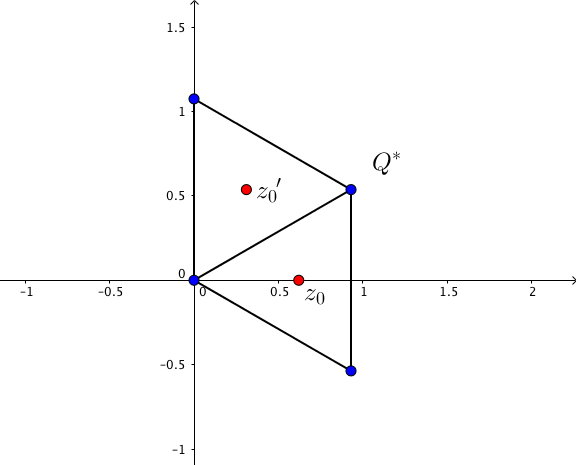
Figure 3: Primitive cell $Q^{*}$ of $\Lambda_{1}^{*}$ formed by two primitive triangle with barycenters $z_{0}$ and $z_{0}^{\prime}$.

For any $\alpha>0$ $z\mapsto\theta_{\Lambda_{1}^{*}+z}(\alpha)$ admits two minimizers in the set $Q^{*}:=[0,1)u_{1}^{*}+[0,1)u_{2}^{*}$, given by Baernstein’s result [6, Thm. 1]. These minimizers are the barycenters of the two primitive triangles forming $Q^{*}$ (see Fig. 3), i.e.

$$z_{0}=\frac{1}{3}(u_{1}^{*}+u_{2}^{*})\quad\textnormal{and}\quad z_{0}^{\prime}=\frac{2}{3}(u_{1}^{*}+u_{2}^{*}).$$ (3.19)

We note that $z_{0}$ and $z_{0}^{\prime}$ belong to $\frac{1}{N}\Lambda_{1}^{*}$ if and only if $N\in 3\mathbb{N}$. Consequently, by Theorem 2.1, the minimum among all the periodic configurations is achieved for any $N\in 3\mathbb{N}$, by the configurations defined, for any $(m,n)\in\mathbb{Z}^{2}$, by

$$\varphi^{*}_{\rm tri}(mu_{1}+nu_{2})=c\cos(2\pi(mu_{1}+nu_{2})\cdot z_{0})=c\cos\left(\frac{2\pi}{3}(m+n)\right).$$

The value $c=\sqrt{2}$ then follows from (2.1).

3.4 Proof of Theorem 2.7

We first show that

$$F[k]=\textnormal{Z}\left|\hskip-2.5pt\begin{array}[]{r}0\@arraycr A_{X}^{t}\frac{k}{N}\end{array}\hskip-2.5pt\right|(q_{X};s)+\frac{2\pi^{\frac{s}{2}}}{s\Gamma(\frac{s}{2})},$$ (3.21)

where $F[k]$ is given in (3.7). Using (1.8), we calculate

$$\pi^{-\frac{s}{2}}\Gamma(\frac{s}{2})\textnormal{Z}\left|\hskip-2.5pt\begin{array}[]{r}0\@arraycr A_{X}^{t}\frac{k}{N}\end{array}\hskip-2.5pt\right|(q_{X};s)+\frac{2}{s}$$ (3.23)

$$\qquad=\int_{1}^{\infty}\sum_{n\in\mathbb{Z}^{d}\backslash\{0\}}e^{2i\pi n\cdot A_{X}^{t}\frac{k}{N}}e^{-\pi tq_{X}(n)}t^{\frac{s}{2}-1}dt+\int_{1}^{\infty}\sum_{n\in\mathbb{Z}^{d}}e^{-\pi tq_{X^{*}}(n+A_{x}^{t}\frac{k}{N})}t^{\frac{d-s}{2}-1}dt,$$

$$\qquad=\int_{1}^{\infty}\sum_{x\in X\backslash\{0\}}e^{2i\pi x\cdot\frac{k}{N}}e^{-\pi t|x|^{2}}t^{\frac{s}{2}-1}dt+\int_{1}^{\infty}\sum_{x\in X^{*}}e^{-\pi t|x+\frac{k}{N}|^{2}}t^{\frac{d-s}{2}-1}dt,$$

Now, we know (see e.g. [56, Eq. (1.9)]) that if $f_{s}(x)=|x|^{-s}$, then

$$d\mu_{f_{s}}(t)=\frac{t^{\frac{s}{2}-1}}{\Gamma\left(\frac{s}{2}\right)}dt.$$

Therefore, in view of (3.14) for $\alpha=\sqrt{\pi}$, we hence get (3.21) by a straightforward computation. Therefore, substituting $F[k]$ in (3.13), we finally obtain

$${\mathcal{E}}_{X,f_{s}}[\varphi] =\frac{1}{2N^{d}}\sum_{k\in K_{N}^{*}}\xi_{k}\textnormal{Z}\left|\hskip-2.5pt\begin{array}[]{r}0\@arraycr A_{X}^{t}\frac{k}{N}\end{array}\hskip-2.5pt\right|(q_{X};s)+\frac{1}{2N^{d}}\sum_{k\in K_{N}^{*}}\xi_{k}\frac{2\pi^{\frac{s}{2}}}{s\Gamma(\frac{s}{2})}-\frac{\pi^{s/2}}{s\Gamma(\frac{s}{2})}$$

$$=\frac{1}{2N^{d}}\sum_{k\in K_{N}^{*}}\xi_{k}\textnormal{Z}\left|\hskip-2.5pt\begin{array}[]{r}0\@arraycr A_{X}^{t}\frac{k}{N}\end{array}\hskip-2.5pt\right|(q_{X};s)+\frac{\pi^{\frac{s}{2}}}{s\Gamma(\frac{s}{2})N^{d}}\left(\sum_{k\in K_{N}^{*}}\xi_{k}-N^{d}\right)$$

$$=\frac{1}{2N^{d}}\sum_{k\in K_{N}^{*}}\xi_{k}\textnormal{Z}\left|\hskip-2.5pt\begin{array}[]{r}0\@arraycr A_{X}^{t}\frac{k}{N}\end{array}\hskip-2.5pt\right|(q_{X};s)$$

by (3.4).

Acknowledgements.

LB is grateful for the support of MATCH during his stay in Heidelberg. Both authors would like to thank Florian Nolte for interesting discussions.

References

- [1] A. Aftalion, X. Blanc, and F. Nier. Lowest Landau level functional and Bargmann spaces for Bose–Einstein condensates. Journal of Functional Analysis, 241:661–702, 2006.
- [2] A. Alastuey and B. Jancovici. On the classical two-dimensional one-component Coulomb plasma. Journal de Physique, 42(1):1–12, 1981.
- [3] M. Antlanger, G. Kahl, M. Mazars, L. Samaj, and E. Trizac. Rich polymorphic behavior of Wigner bilayers. Physical Review Letters, 117(11):118002, 2016.
- [4] L. Assoud, R. Messina, and H. Löwen. Stable crystalline lattices in two-dimensional binary mixtures of dipolar particles. Europhysics Letters, 80(4):1–6, 2007.
- [5] G. Bachman, L. Narici, and E. Beckenstein. Fourier and wavelet analysis. Springer, Berlin, 2002.
- [6] A. Baernstein II. A minimum problem for heat kernels of flat tori. Contemporary Mathematics, 201:227–243, 1997.
- [7] S. Bernstein. Sur les fonctions absolument monotones. Acta Math., 52:1–66, 1929.
- [8] L. Bétermin. Two-dimensional Theta Functions and Crystallization among Bravais Lattices. SIAM J. Math. Anal., 48(5):3236–3269, 2016.
- [9] L. Bétermin. Local optimality of cubic lattices for interaction energies. Anal. Math. Phys., (online first) DOI:10.1007/s13324-017-0205-5, 2017.
- [10] L. Bétermin and H. Knüpfer. Optimal lattice configurations for interacting spatially extended particles. Letters in Mathematical Physics, (online first) DOI: 10.1007/s11005-018-1077-9, 2018.
- [11] L. Bétermin and M. Petrache. Dimension reduction techniques for the minimization of theta functions on lattices. J. Math. Phys., 58:071902, 2017.
- [12] L. Bétermin and E. Sandier. Renormalized Energy and Asymptotic Expansion of Optimal Logarithmic Energy on the Sphere. Constr. Approx. , Special Issue: Approximation and Statistical Physics - Part I, 47(1):39–74, 2018.
- [13] L. Bétermin and P. Zhang. Minimization of energy per particle among Bravais lattices in : Lennard-Jones and Thomas-Fermi cases. Commun. Contemp. Math., 17(6):1450049, 2015.
- [14] X. Blanc and M. Lewin. The Crystallization Conjecture: A Review. EMS Surveys in Mathematical Sciences, 2:255–306, 2015.
- [15] S. Bochner. Theta relations with spherical harmonics. Proc. Natl. Acad. Sci. U.S.A., 37(12):804–808, 1951.
- [16] M. Born. Über elektrostatische Gitterpotentiale. Zeitschrift für Physik, 7:124–140, 1921.
- [17] J. M. Borwein, M. L. Glasser, R. C. McPhedran, J. G. Wan, and I. J. Zucker. Lattice sums: then and now. volume 150 of Encyclopedia of Mathematics, 2013.
- [18] N. Bouman, J. Draisma, and J. S. H. Van Leeuwaarden. Energy minimization of repelling particles on a toric grid. SIAM J. Discrete Math., 27(3):1295–1312, 2013.
- [19] J.W.S. Cassels. On a Problem of Rankin about the Epstein Zeta-Function. Proceedings of the Glasgow Mathematical Association, 4:73–80, 7 1959.
- [20] H. Cohn and A. Kumar. Universally optimal distribution of points on spheres. J. Amer. Math. Soc., 20(1):99–148, 2007.
- [21] J. H. Conway and N. J. A. Sloane. Sphere Packings, Lattices and Groups, volume 290. Springer, 1999.
- [22] R. Coulangeon. Spherical Designs and Zeta Functions of Lattices. International Mathematics Research Notices, ID 49620(16), 2006.
- [23] R. Coulangeon and G. Lazzarini. Spherical Designs and Heights of Euclidean Lattices. Journal of Number Theory, 141:288–315, 2014.
- [24] R. Coulangeon and A. Schürmann. Energy Minimization, Periodic Sets and Spherical Designs. International Mathematics Research Notices, pages 829–848, 2012.
- [25] R. Coulangeon and A. Schürmann. Local Energy Optimality of Periodic Sets. Preprint. arXiv:1802.02072, 2018.
- [26] S. W. de Leeuw, J. W. Perram, and E.R. Smith. Simulation of Electrostatic Systems in Periodic Boundary Conditions. I. Lattice Sums and Dielectric Constants. Proceedings of the Royal Society of London A: Mathematical, Physical and Engineering Sciences, 373(1752):27–56, 1980.
- [27] P. H. Diananda. Notes on Two Lemmas concerning the Epstein Zeta-Function. Proceedings of the Glasgow Mathematical Association, 6:202–204, 7 1964.
- [28] W. E and D. Li. On the Crystallization of 2D Hexagonal Lattices. Communications in Mathematical Physics, 286:1099–1140, 2009.
- [29] O. Emersleben. Zetafunktionen und elektrostatische Gitterpotentiale. I. Phys. Z., 24:73–80, 1923.
- [30] V. Ennola. A Lemma about the Epstein Zeta-Function. Proceedings of The Glasgow Mathematical Association, 6:198–201, 1964.
- [31] P. Epstein. Zur Theorie allgemeiner Zetafunctionen. Mathematische Annalen, 56(4):615–644, 1903.
- [32] P. Ewald. Die Berechnung optischer und elektrostatischer Gitterpotentiale. Annalen der physik, 64:253–287, 1921.
- [33] M. Faulhuber and S. Steinerberger. Optimal gabor frame bounds for separable lattices and estimates for jacobi theta functions. Journal of Mathematical Analysis and Applications, 445(1):407–422, 2017.
- [34] L. Flatley and F. Theil. Face-Centred Cubic Crystallization of Atomistic Configurations. Archive for Rational Mechanics and Analysis, 219(1):363–416, 2015.
- [35] D. P. Hardin, E. B. Saff, and Brian Simanek. Periodic Discrete Energy for Long-Range Potentials. Journal of Mathematical Physics, 55(12):123509, 2014.
- [36] M. B. Hay, R. K. Workman, and S. Manne. Two-dimensional condensed phases from particles with tunable interactions. Physical Review E, 67(1), 2003.
- [37] R. C. Heitmann and C. Radin. The Ground State for Sticky Disks. Journal of Statistical Physics, 22:281–287, 1980.
- [38] A. Henn. The Hexagonal Lattice and the Epstein Zeta Function. Dynamical Systems, Number Theory and Applications A Festschrift in Honor of Armin Leutbecher’s 80th Birthday (Chapter 7), 2016.
- [39] A. Krazer and E. Prym. Neue Grundlagen einer Theorie der Allgemeinen Theta-funktionen. Teubner, Leipzig, 1893.
- [40] V. A. Levashov, M. F. Thorpe, and B. W. Southern. Charged lattice gas with a neutralizing background. Physical Review B, 67(22), 2003.
- [41] L. De Luca and G. Friesecke. Crystallization in two dimensions and a discrete gauss-bonnet theorem. J. Nonlinear Sci., 28(1):69–90, 2018.
- [42] E. Mainini, P. Piovano, and U. Stefanelli. Finite crystallization in the square lattice. Nonlinearity, 27:717–737, 2014.
- [43] E. Mainini and U. Stefanelli. Crystallization in carbon nanostructures. Comm. Math. Phys., 328:545–571, 2014.
- [44] H. L. Montgomery. Minimal Theta Functions. Glasgow Mathematical Journal, 30(1):75–85, 1988.
- [45] E. J. Mueller and T.-L. Ho. Two-Component Bose-Einstein Condensates with a Large Number of Vortices. Physical Review Letters, 88(18), 2002.
- [46] S. Nonnenmacher and A. Voros. Chaotic Eigenfunctions in Phase Space. Journal of Statistical Physics, 92:431–518, 1998.
- [47] O. N. Osychenko, G. E. Astrakharchik, and J. Boronat. Ewald method for polytropic potentials in arbitrary dimensionality. Mol. Phys., 110(4):227–247, 2012.
- [48] L. Pauling. The principles determining the structure of complex ionic crystals. J. Am. Chem. Soc., 51(4):1010–1026, 1929.
- [49] J.W. Perram and S.W. de Leeuw. Statistical mechanics of two-dimensional coulomb systems. I. Lattice sums and simulation methodology. Physica A: Statistical Mechanics and Its Applications, 109(1-2):237–250, 1981.
- [50] C. Radin. The Ground State for Soft Disks. Journal of Statistical Physics, 26(2):365–373, 1981.
- [51] R. A. Rankin. A Minimum Problem for the Epstein Zeta-Function. Proceedings of The Glasgow Mathematical Association, 1:149–158, 1953.
- [52] N. Rougerie and S. Serfaty. Higher dimensional coulomb gases and renormalized energy functionals. Communications on Pure and Applied Mathematics, 69(3):519–605, 2016.
- [53] L. Samaj and E. Trizac. Critical phenomena and phase sequence in a classical bilayer wigner crystal at zero temperature. Physical Review B, 85(20), 2012.
- [54] E. Sandier and S. Serfaty. From the Ginzburg-Landau Model to Vortex Lattice Problems. Communications in Mathematical Physics, 313(3):635–743, 2012.
- [55] P. Sarnak and A. Strömbergsson. Minima of Epstein’s Zeta Function and Heights of Flat Tori. Inventiones Mathematicae, 165:115–151, 2006.
- [56] J. L. Schiff. The Laplace transform: theory and applications. Springer Science and Business Media, 2013.
- [57] E. M. Stein and R. Shakarchi. Complex Analysis. Princeton University Press, 2003.
- [58] F. Theil. A Proof of Crystallization in Two Dimensions. Communications in Mathematical Physics, 262(1):209–236, 2006.
- [59] W.J. Ventevogel. On the Configuration of Systems of Interacting Particle with Minimum Potential Energy per Particle. Physica A-statistical Mechanics and Its Applications, 92A:343, 1978.
- [60] W.J. Ventevogel and B.R.A. Nijboer. On the Configuration of Systems of Interacting Particle with Minimum Potential Energy per Particle. Physica A-statistical Mechanics and Its Applications, 98A:274–288, 1979.
- [61] Y. Xiao, M. F. Thorpe, and J. B. Parkinson. Two-dimensional discrete coulomb alloy. Physical Review B, 59(1):277–285, 1999.