Tiling functions and Gabor orthonormal basis

Abstract

We study the existence of Gabor orthonormal bases with window the characteristic function of the set $\Omega=[0,\alpha]\cup[\beta+\alpha,\beta+1]$ of measure 1, with $\alpha,\beta>0$. By the symmetries of the problem, we can restrict our attention to the case $\alpha\leq 1/2$. We prove that either if $\alpha<1/2$ or ($\alpha=1/2$ and $\beta\geq 1/2$) there exist such Gabor orthonormal bases, with window the characteristic function of the set $\Omega$, if and only if $\Omega$ tiles the line. Furthermore, in both cases, we completely describe the structure of the set of time-frequency shifts associated to these bases.

Keywords: Spectral sets; Fuglede’s Conjecture; Tilings; Packings; Gabor basis
AMS 2010 Mathematics Subject Classification: Primary: 42C99, 52C22

1 Introduction

In this note we study the Gabor orthonormal basis having as window a characteristic function of a union of two intervals on $\mathbb{R}$, of the form

$$\Omega=[0,\alpha]\cup[\beta+\alpha,\beta+1],$$ (1)

and $|\Omega|=1$. By the symmetries of the problem, we can restrict our attention to the case where $\alpha\in(0,1/2]$ and $\beta>0$.

This paper draws on the ideas and some results given in [5], where the structure of Gabor bases with the window being the unit cube has been studied in general space of dimension $d$, producing surprising results even from dimension $d=2$. Here we restrict ourselves to space dimension $d=1$ but we vary the window in the simplest possible way: we examine the situation when the window is the indicator function of a union of two intervals satisfying (1).

First we characterize the Gabor orthonormal basis for a general function $g\in L^{2}(\mathbb{R}^{d})$ in terms of a tiling condition involving the short time Fourier transform (of the window with respect to itself) also known as Gabor transform (see Theorem 3.1). This condition is completely analogous to the characterization of domain spectra, in the study of the so-called Fuglede conjecture (see, for instance, [9, Theorem 3.1]). Our main result is Theorem 4.3 which provides the geometric conditions that characterize the Gabor orthonormal basis of $\chi_{\Omega}$ where $\Omega$ is given by (1), and $\alpha<1/2$ or ($\alpha=1/2$ and $\beta\geq 1/2$).

As a consequence of Theorem 4.3 we can relate the existence of Gabor orthonormal bases using $\chi_{\Omega}$ with tiling properties of the set $\Omega$. Recall that we say that a set $\Omega\subseteq\mathbb{R}^{d}$ tiles $\mathbb{R}^{d}$ if

$$\sum_{\lambda\in\Lambda}\chi_{\Omega}(x-\lambda)=1$$

almost everywhere for some set $\Lambda\subseteq\mathbb{R}^{d}$. In [3] $\L$aba proved that for the union of two intervals the Fuglede conjecture is true. In particular, the tiling condition implies the existence of an orthonormal basis $\{e^{2\pi i\lambda\cdot}\}_{\lambda\in\Lambda}$ for $L^{2}(\Omega)$. The set of frequencies $\Lambda$ is called a spectrum for $\Omega$. Moreover, she proved that $\Omega$ tiles the real line, and therefore it has a spectrum, if and only if $\alpha$ and $\beta$ satisfy one of the following two conditions:

• $\displaystyle 0<\alpha<1/2$ and $\beta\in\mathbb{N}$;

• $\alpha=1/2$ and $\displaystyle\beta\in\frac{1}{2}\mathbb{N}$.

The sets $\Omega$ given by (i) are (up to translation and reflection) the $\mathbb{Z}$-tiles consisting of two intervals. On the other hand, the sets in the case (ii) are also $\mathbb{Z}$-tiles if $\beta$ is integer, otherwise, if $\displaystyle\beta=\frac{n-1}{2}$, for any even $n\in\mathbb{N}$ these sets are tiles with respect to the set of translations

$$n\mathbb{Z}\cup\left(n\mathbb{Z}+\frac{1}{2}\right)\cup\dots\cup\left(n\mathbb{Z}+\frac{n-1}{2}\right).$$

By $\L$aba’s result, note that either in the case (i) or in the case (ii) there exists Gabor orthonormal basis

$$\{e^{2\pi i\nu\cdot}\chi_{\Omega}(\cdot-t):(t,\nu)\in\Gamma\}$$

where $\Gamma$ can be taken as a product of the set used to tile $\mathbb{R}$ with $\Omega$, and any spectrum $\Lambda$ for $\Omega$. A natural question is whether or not there are other sets $\Omega$ as in (1) that produce Gabor orthonormal basis. As a consequence of Theorem 4.3 we get that, among the sets $\Omega$ that satisfy $\alpha<1/2$ or ($\alpha=1/2$ and $\beta\geq 1/2$), only those which tile the real line can produce Gabor orthonormal bases (Theorem 4.6). Moreover, in these cases we can describe the structure of the sets of time-frequency translations that produce those orthonormal bases (Theorems 4.7 and 4.8).

One of the basic tools in this characterization is the behavior of the zero set of the short time Fourier transform of the characteristic function of $\Omega$, a situation also observed in [5] and which closely mirrors what happens in the related Fuglede problem [9]. Even though, this zero set is completely described in Appendix A, the aim of Appendix A is complementary and it is not directly used in the proof of the main result.

2 Preliminaries

Given $g\in L^{2}(\mathbb{R}^{d})$, and $\lambda=(t,\nu)\in\mathbb{R}^{d}\times\mathbb{R}^{d}$, let $g_{\lambda}$ denote the time-frequency shift of $g$ defined by

$$g_{\lambda}(x)=g(x-t)e^{2\pi i\left\langle\,x,\nu\,\right\rangle}.$$

From now on, $\mathbb{R}^{d}\times\mathbb{R}^{d}$ will be identified with $\mathbb{R}^{2d}$. Let $\Lambda$ be a discrete countable set of $\mathbb{R}^{2d}$. The Gabor system associated to the so-called window $g$ consists of the set of time-frequency shifts $\{g_{\lambda}\}_{\lambda\in\Lambda}$. We are especially interested in the case when a Gabor system is an orthogonal basis (a Gabor basis).

2.1 Short time Fourier transform

In this subsection we will recall the definition and some properties of the short time Fourier transform, also known as Gabor transform. More information can be found in [7].

Definition 2.1.

Given $g\in L^{2}(\mathbb{R}^{d})$, the short time Fourier transform with window $g$ is defined for any $f\in L^{2}(\mathbb{R}^{d})$ by

$$V_{g}f(t,\nu):=\int_{\mathbb{R}^{d}}f(x)\overline{g(x-t)}e^{-2\pi i\left\langle\,x,\nu\,\right\rangle}dx=\left\langle\,f,g_{(t,\nu)}\,\right\rangle.$$ (2)

One of the most useful properties of this transform is the following relation.

Proposition 2.2.

Let $f_{1},f_{2},g_{1},g_{2}\in L^{2}(\mathbb{R}^{d})$. Then, $V_{g_{j}}f_{j}\in L^{2}(\mathbb{R}^{2d})$ for $j=1,2$, and

$$\left\langle\,V_{g_{1}}f_{1},V_{g_{2}}f_{2}\,\right\rangle=\left\langle\,f_{1},f_{2}\,\right\rangle\overline{\left\langle\,g_{1},g_{2}\,\right\rangle}.$$

Corollary 2.3.

If $f,g\in L^{2}(\mathbb{R}^{d})$, then

$$\|V_{g}f\|^{2}_{2}=\|f\|^{2}_{2}\|g\|^{2}_{2}.$$

In particular, if $\|g\|_{2}=1$ then $V_{g}$ is an isometry from $L^{2}(\mathbb{R}^{d})$ into $L^{2}(\mathbb{R}^{2d})$.

Another consequence is the following result.

Corollary 2.4.

Let $f,g\in L^{2}(\mathbb{R}^{d})$ such that $g\neq 0$ in $L^{2}$. If $\left\langle\,f,g_{\omega}\,\right\rangle=0$ for every $\omega\in\mathbb{R}^{2d}$, then $f=0$ in $L^{2}$.

We conclude this section with the following proposition that provides the behavior of Gabor transforms with respect to time-frequency shifts.

Proposition 2.5.

Given $f,g\in L^{2}(\mathbb{R}^{d})$ and $\lambda=(t,\omega)\in\mathbb{R}^{2d}$

$$V_{g}\,f_{\lambda}\,(x,\nu)=e^{-2\pi i\left\langle\,t,\nu-\omega\,\right\rangle}V_{g}f(x-t,\nu-w).$$

2.2 Tilings

Let $\delta_{\lambda}$ be the unit point mass sitting at the point $\lambda\in\mathbb{R}^{n}$. Recall that, given a function $h\geq 0$, the convolution $h*\delta_{\lambda}(x)$ in the distribution sense gives the translation $h(x-\lambda)$. Let $\delta_{\Lambda}$ denote the measure

$$\delta_{\Lambda}=\sum_{\lambda\in\Lambda}\delta_{\lambda},$$

where $\Lambda$ is a discrete set of $\mathbb{R}^{n}$. Then, if

$$\delta_{\Lambda}*h(x)=\sum_{\lambda\in\Lambda}h(x-\lambda)=1,$$

for almost every $x\in\mathbb{R}^{n}$, we say that $h$ tiles $\mathbb{R}^{n}$ with translation set $\Lambda\subseteq\mathbb{R}^{n}$. If, for example, $h=\chi_{\Omega}$, where $\Omega$ is a measurable subset of $\mathbb{R}^{n}$ then the tiling condition means that

$$\lambda+\Omega:=\{\omega+\lambda:\,\omega\in\Omega\},\quad\text{ \rm where }\quad\lambda\in\Lambda$$

intersect each other in a set of zero Lebesgue measure, and their union covers the whole space except perhaps for a set of measure zero. We often denote the situation $h*\delta_{\Lambda}=1$ (tiling) by

$$h+\Lambda=\mathbb{R}^{d}.$$

Similarly we say that $h+\Lambda$ is a packing, and we denote this by

$$h+\Lambda\leq\mathbb{R}^{d},$$

if $h*\delta_{\Lambda}\leq 1$ almost everywhere. If $h=\chi_{\Omega}$, we also use the notation

$$\Omega+\Lambda\leq\mathbb{R}^{d}$$

for packing and

$$\Omega+\Lambda=\mathbb{R}^{d}$$

for tiling.

3 Orthogonality and the zero set of Gabor transform

Throughout this section $\Lambda$ will denotes a discrete subset of $\mathbb{R}^{2d}$. Given a Borel set $\Omega$, which has finite measure, the orthogonality of exponential families in $L^{2}(\Omega)$ can be studied using the Fourier transform of $\chi_{\Omega}$. In this section we will show that there exists a similar connection between the orthogonality properties of a Gabor system $\{g_{\lambda}\}_{\Lambda}$ and the zero set of $V_{g}g$.

Theorem 3.1.

Given $g\in L^{2}(\mathbb{R}^{d})$ and $\|g\|_{2}=1$, the following statements are equivalent:

• The Gabor system $\{g_{\lambda}\}_{\Lambda}$ forms an orthonormal system.

• $\displaystyle\sum_{\lambda\in\Lambda}|V_{g}f(\omega-\lambda)|^{2}\leq 1,$ for every $f\in L^{2}(\mathbb{R}^{d})$ so that $\|f\|_{2}=1$, and $\omega\in\mathbb{R}^{2d}$. In other words

  $$|V_{g}f|^{2}+\Lambda\ \ \ \mbox{is a packing}.$$

• $\displaystyle\sum_{\lambda\in\Lambda}|V_{g}g(\omega-\lambda)|^{2}\leq 1,$ for every $\omega\in\mathbb{R}^{2d}$. In other words

  $$|V_{g}g|^{2}+\Lambda\ \ \ \ \mbox{is a packing}.$$

We also have that the following are equivalent:

• The Gabor system $\{g_{\lambda}\}_{\Lambda}$ forms an orthonormal basis.

• $\displaystyle\sum_{\lambda\in\Lambda}|V_{g}f(\omega-\lambda)|^{2}=1,$ for every $f\in L^{2}(\mathbb{R}^{d})$ so that $\|f\|_{2}=1$, and $\omega\in\mathbb{R}^{2d}$. In other words

  $$|V_{g}f|^{2}+\Lambda\ \ \ \mbox{is a tiling}.$$

• $\displaystyle\sum_{\lambda\in\Lambda}|V_{g}g(\omega-\lambda)|^{2}=1,$ for every $\omega\in\mathbb{R}^{2d}$. In other words

  $$|V_{g}g|^{2}+\Lambda\ \ \ \ \mbox{is a tiling}.$$

Proof.

Let us first prove the equivalence of (i), (ii) and (iii). Clearly (ii) $\Rightarrow$ (iii). Hence, it is enough to show that (i) $\Rightarrow$ (ii) and (iii) $\Rightarrow$ (i).

(i) $\Rightarrow$ (ii) Assume that $\{g_{\lambda}\}_{\lambda\in\Lambda}$ forms an orthonormal system for $L^{2}(\mathbb{R}^{d})$. Since

$$|\left\langle\,g_{\lambda_{1}},g_{\lambda_{2}}\,\right\rangle|=|\left\langle\,g_{-\lambda_{1}},g_{-\lambda_{2}}\,\right\rangle|,$$ (3)

the Gabor system $\{g_{-\lambda}\}_{\lambda\in\Lambda}$ is also orthonormal. Then, by the Bessel’s inequality,

$$1\geq\sum_{\lambda\in\Lambda}|\left\langle\,f,g_{-\lambda}\,\right\rangle|^{2}=\sum_{\lambda\in\Lambda}|V_{g}f(-\lambda)|^{2},$$ (4)

for every $f\in L^{2}(\mathbb{R}^{d})$, so that $\|f\|_{2}=1$. By Proposition 2.5, if $\omega\in\mathbb{R}^{2d}$ and replacing $f$ by $f_{-\omega}$, we get

$$1\geq\sum_{\lambda\in\Lambda}|\left\langle\,f_{-\omega},g_{-\lambda}\,\right\rangle|^{2}=\sum_{\lambda\in\Lambda}|V_{g}f(\omega-\lambda)|^{2}.$$

(iii) $\Rightarrow$ (i) First of all, note that taking $w=\lambda_{0}$ for some $\lambda_{0}\in\Lambda$ we obtain

$$|V_{g}(0)|^{2}+\sum_{\lambda\neq\lambda_{0}}|V_{g}g(\lambda_{0}-\lambda)|^{2}\leq 1.$$

Since $V_{g}g(0)=\|g\|_{2}^{2}=1$, we get that for every $\lambda\in\Lambda\setminus\{\lambda_{0}\}$

$$0=|V_{g}g(\lambda_{0}-\lambda)|=|\left\langle\,g_{\lambda_{0}},g_{\lambda}\,\right\rangle|.$$

Therefore, $\{g_{\lambda}\}_{\lambda\in\Lambda}$ is an orthonormal system.

Now, assume (vi). It follows from the equivalence of (i), (ii) and (iii) that the Gabor system is orthonormal. In order to prove that the Gabor system is complete it is enough to prove that

$$\sum_{\lambda\in\Lambda}|\left\langle\,f,g_{\lambda}\,\right\rangle|^{2}=1$$

for a set of norm one elements $f\in L^{2}(\mathbb{R}^{d})$ that is dense in the sphere of $L^{2}(\mathbb{R}^{d})$. By (3) and the hypothesis we know that for every $\omega\in\mathbb{R}^{2d}$

$$\sum_{\lambda\in\Lambda}|\left\langle\,g_{\omega},g_{\lambda}\,\right\rangle|^{2}=\sum_{\lambda\in\Lambda}|\left\langle\,g_{-\omega},g_{-\lambda}\,\right\rangle|^{2}=\sum_{\lambda\in\Lambda}|V_{g}g(\omega-\lambda)|^{2}=1.$$

By Corollary 2.4 the family $\{g_{\omega}\}_{\omega\in\mathbb{R}^{2d}}$ is complete. So $\{g_{\lambda}\}_{\lambda\in\Lambda}$ is an orthonormal basis. $\blacksquare$

As is the case of Fuglede problem [9] orthogonality alone of a set $\Lambda$ can be decided by looking at the difference set and making sure that it is contained in the zero set of the short time Fourier transform given by:

$$\mathcal{Z}(V_{g}g)=\{(t,\nu):V_{g}g(t,\nu)=0\}.$$

Corollary 3.2.

Let $g\in L^{2}(\mathbb{R}^{d})$ such that $\|g\|_{2}=1$. The following statements are equivalent:

1. The Gabor system $\{g_{\lambda}\}_{\lambda\in\Lambda}$ is orthonormal;

2. $\Lambda-\Lambda\subseteq\mathcal{Z}(V_{g}g)\cup\{0\}$.

3.1 Packing regions

By Theorem 3.1, for $\|g\|_{2}=1$, the Gabor system $\{g_{\lambda}\}_{\lambda\in\Lambda}$ is orthonormal if and only if

$$|V_{g}g|^{2}+\Lambda\leq 1$$

In order to determine when this system is also complete, and so $\{g_{\lambda}\}$ is an orthonormal basis, we have to decide whether or not the equality

$$|V_{g}g|^{2}+\Lambda=1$$

holds. In general, it is easier to prove that a characteristic function tiles with some set $\Lambda$ than to prove that $|V_{g}g|^{2}$ tiles with $\Lambda$. The following simple lemma enables us to check the tiling properties of $|V_{g}g|^{2}$ by proving the tiling properties of some characteristic functions:

Lemma 3.3.

Let $F,G\in L^{1}(\mathbb{R}^{d})$ be two functions so that $F,G\geq 0$ and

$$\int_{\mathbb{R}^{d}}F(x)dx=\int_{\mathbb{R}^{d}}G(x)dx=1.$$

Let $\mu$ be a positive Borel measure on $\mathbb{R}^{d}$ so that $F*\mu\leq 1$ and $G*\mu\leq 1$. Then, $F*\mu=1$ if and only if $G*\mu=1$.

So, we can replace $|V_{g}g|^{2}$ by a simpler function. The proof of this result, as well as the next definition, can be found for instance in [5] (see also the references therein).

Definition 3.4.

Given $g\in L^{2}(\mathbb{R}^{d})$, a region $D\subset\mathbb{R}^{2d}$ is an (orthogonal) packing region for $g$ if

$$(D^{\circ}-D^{\circ})\cap\mathcal{Z}(V_{g}g)=\varnothing,$$

where $D^{\circ}$ denotes the interior of $D$. If $\|g\|_{2}=1$ then the orthogonal packing region $D$ is called tight when $|D|=1$.

A simple computation shows that if $D$ is a packing region for $g$ then

$$D+\Lambda\leq\mathbb{R}^{d}$$

for any $\Lambda$ such that $\Lambda-\Lambda\subseteq\mathcal{Z}(V_{g}g)$. Hence, by Lemma 3.3, in order to prove that $|V_{g}g|^{2}$ tiles $\mathbb{R}^{2d}$ with $\Lambda$ it is enough to find a tight packing region and prove that $D$ tiles $\mathbb{R}^{2d}$ with $\Lambda$. More precisely

Theorem 3.5.

Let $g$ be a norm-one element of $L^{2}(\mathbb{R}^{d})$, $D$ is a tight packing region for $g$, and $\Lambda$ a discrete set such that $\{g_{\lambda}\}_{\lambda\in\Lambda}$ is an orthonormal system. Then the following statements are equivalent:

• The system $\{g_{\lambda}\}_{\lambda\in\Lambda}$ is an orthonormal basis of $L^{2}(\mathbb{R}^{d})$

• The tight packing region $D$ tiles $\mathbb{R}^{2d}$ with $\Lambda$.

Although to prove the tiling properties of $\chi_{D}$ is easier than to prove the tiling properties of $|V_{g}g|^{2}$, the issue now is to find such a tight packing region when it exists.

4 The case of two intervals

In this section we study Gabor orthonormal bases generated by the characteristic function $g=\chi_{\Omega}$, where $\Omega$ is the union of two intervals. The orthonormality condition imposes that $|\Omega|=1$, and using the symmetries of the problem, we can restrict our attention to sets of the form

$$\Omega=[0,\alpha)\cup[\alpha+\beta,1+\beta),\quad\quad\mbox{with $\alpha\in[0,1/2]$, and $\beta>0$}.$$ (5)

If $\alpha<1/2$ we characterize all the possible values of $\beta$, such that for some $\Lambda$, the family $\{g_{\lambda}\}_{\lambda\in\Lambda}$ forms an orthonormal basis. In particular, we prove that there exists $\Lambda$ such that $\{g_{\lambda}\}_{\lambda\in\Lambda}$ forms an orthonormal basis if and only if $\Omega$ tiles $\mathbb{R}$ (see Theorem 4.6). Moreover, we show that in this case the set $\Lambda$ has a very precise structure (see Theorem 4.7). If $\alpha=1/2$, we also give a characterization of all the possible values of $\beta$, but this time assuming that $\beta\geq 1/2$ (see also Theorem 4.6). The case $\alpha=1/2$ and $\beta<1/2$ remains open. To begin with, we present the results, and we leave the proofs for the next two subsections.

Our first goal is to provide a geometric characterization of the Gabor orthonormal basis $\{g_{\lambda}\}_{\lambda\in\Lambda}$ when $g=\chi_{\Omega}$ and $\Omega$ has the form shown in (5). With this aim, we prove that $\chi_{\Omega}$ admits a tight orthogonal packing region provided $\alpha<1/2$ or ($\alpha=1/2$ and $\beta\geq 1/2$).

Theorem 4.1.

Let $\Omega=[0,\alpha)\cup[\alpha+\beta,1+\beta)$, where $\alpha\in(0,1/2)$ and $\beta>0$. Then, the set

$$D=\Omega\times[0,1)=\Big{(}[0,\alpha)\cup[\alpha+\beta,1+\beta)\Big{)}\times[0,1)$$

forms a tight orthogonal packing region for $\chi_{\Omega}$.

When both intervals of $\Omega$ have the same length, the structure of the zero set of $V_{\chi_{\Omega}}\chi_{\Omega}$ is more complicated. So the packing region is more complicated too.

Theorem 4.2.

Let $\Omega=[0,1/2)\cup[1/2+\beta,\beta+1)$ so that $\beta\geq 1/2$. Then, a tight orthogonal packing region for $\chi_{\Omega}$ is

$$D=\begin{cases}\displaystyle\Omega\times\left(\bigcup_{k=0}^{2\beta}\left[\frac{2k}{2\beta+1},\frac{2k+1}{2\beta+1}\right)\right)&\mbox{if $\beta\in\frac{1}{2}\mathbb{N}$}\\ \displaystyle\Omega\times\left(\bigcup_{k=0}^{\lfloor 2\beta\rfloor}\left[\frac{2k}{2\beta+1},\frac{2k+1}{2\beta+1}\right)\cup\left[\frac{2(\lfloor 2\beta\rfloor+1)}{2\beta+1},\frac{2(\lfloor 2\beta\rfloor+1)+\{2\beta\}}{2\beta+1}\right)\right)&\mbox{if $\beta\notin\frac{1}{2}\mathbb{N}$}\end{cases}$$

where $\lfloor x\rfloor$ denotes the (floor) integer part of $x$ and $\{x\}=x-\lfloor x\rfloor$.

Note that in order to construct $D$, we first consider the set $\Omega\times\big{[}0,\frac{1}{2\beta+1}\big{)}$. Then, we translate it along the axis of $y$ by $\frac{2k}{2\beta+1}$ where $k=1,\dots,2\beta$ if $\beta\in\frac{1}{2}\mathbb{N}$. The set $D$ is just the union of $\Omega\times\big{[}0,\frac{1}{2\beta+1}\big{)}$ and its translates (see next picture).

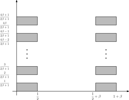
Figure 1: The set $D$ when $\beta\in\frac{\mathbb{N}}{2}$

In the case $\beta\notin\frac{1}{2}\mathbb{N}$, we proceed in a similar way: we consider the set $\Omega\times\big{[}0,\frac{1}{2\beta+1}\big{)}$ and translate it by $\frac{2k}{2\beta+1}$ where $k=1,\dots,\lfloor 2\beta\rfloor$. However, the union of these sets is not of measure 1. So, in order to form $D$ so that $|D|=1$, we have to consider the union of the previous sets and we should also add the set

$$\Omega\times\left[\frac{2(\lfloor 2\beta\rfloor+1)}{2\beta+1},\frac{2(\lfloor 2\beta\rfloor+1)+\{2\beta\}}{2\beta+1}\right).$$

This last set is the union of the thinner sets in the next picture.

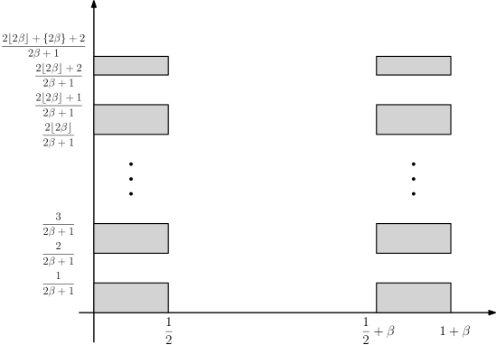
Figure 2: The set $D$ when $\beta\notin\frac{\mathbb{N}}{2}$

The proofs of Theorems 4.1 and 4.2 are left for the subsections 4.1 and 4.2. Now, by Corollary 3.2 and Theorem 3.5, Theorems 4.1 and 4.2 directly lead to the following geometric characterization of the sets $\Lambda$ that produce Gabor orthonormal basis, which is the main result of this paper.

Theorem 4.3.

Let $g=\chi_{\Omega}$, where $\Omega=[0,\alpha)\cup[\beta+\alpha,\beta+1)$, where $\alpha<1/2$ or ($\alpha=1/2$ and $\beta\geq 1/2$). Then $\{g_{\lambda}\}_{\lambda\in\Lambda}$ forms an orthonormal basis if and only if

• $\Lambda-\Lambda\subset\mathcal{Z}(V_{g}g)\cup\{0\}$,

• $\Lambda+D=\mathbb{R}^{2}$,

where $D$ is the tight othogonal packing region described by Theorem 4.1 or Theorem 4.2 depending on the case.

Remark 4.4.

When $\alpha=1/2$ and $\beta<1/2$, the structure of the zero set of $V_{\chi_{\Omega}}\chi_{\Omega}$ is even more complicated. From the computations that we will show in Subsection 4.2 it follows that

$$D=[0,1+\beta)\times[0,(1+2\beta)^{-1})$$

is a packing region for $\chi_{\Omega}$. However $|D|<1$. We could not prove the existence of a tight packing region. So, our techniques can not be applied in this case. $\blacktriangle$

Gabor orthonormal basis and tiling properties of $\Omega$

Our next goal is to relate the existence of Gabor orthonormal basis having as window the function $\chi_{\Omega}$ with some tiling properties of $\Omega$. In [3], $\L$aba proved that the Fuglede conjecture is true for the union of two intervals. Thus, if a set $\Omega$ tiles the real line with some set $\Gamma$, then it is also spectral, which means that $L^{2}(\Omega)$ admits an orthonormal basis of exponentials $\{e_{\lambda}\}_{\lambda\in\Lambda}$. More precisely she got the next result:

Theorem 4.5.

Let $\Omega$ be a union of two intervals as in equation (5). Then $\Omega$ tiles the real line if and only if it is spectral. Moreover, this happens either if $\alpha<1/2$ and $\beta\in\mathbb{Z}$ or if $\alpha=1/2$ and $\beta\in\frac{1}{2}\mathbb{Z}$.

As a consequence of Theorem 4.3 and Fubini’s theorem we get the following result.

Theorem 4.6.

Let $\Omega=[0,\alpha)\cup[\alpha+\beta,1+\beta)$, where $\alpha<1/2$ or ($\alpha=1/2$ and $\beta\geq 1/2$). Then, there exists a Gabor orthonormal basis associated to the function $\chi_{\Omega}$ if and only if $\Omega$ tiles the real line. This occurs exactly when any of the following conditions holds:

• $\displaystyle 0<\alpha<1/2$ and $\beta\in\mathbb{N}$;

• $\alpha=1/2$ and $\displaystyle\beta\in\frac{1}{2}\mathbb{N}$.

Proof.

Let $g=\chi_{\Omega}$. Let $\Lambda$ be a subset of $\mathbb{R}^{2}$ so that $\{g_{\lambda}\}_{\lambda\in\Lambda}$ is a Gabor orthonormal basis. By Theorem 4.3 we get that $D+\Lambda=\mathbb{R}^{2}$, where $D$ is a tight orthogonal packing region (explicitly given in Theorems 4.1 and 4.2). Since $D$, which is a Cartesian product of $\Omega$ with another set, tiles $\mathbb{R}^{2}$, by Fubini’s theorem $\Omega$ must tile the line. The description of such sets is given in [3]. The converse is easier, because if $\Omega$ tiles the real line, it also admits a spectrum (see [3]). Therefore, as we mentioned in the introduction, there exists a set $\Lambda$ so that $\{g_{\lambda}\}_{\lambda\in\Lambda}$ is a Gabor orthonormal basis. $\blacksquare$

Let $\displaystyle g=\chi_{\Omega}$, where $\Omega\subset\mathbb{R}^{d}$ is measurable of measure 1. Suppose that

$$\Lambda=\bigcup_{t\in J}\{t\}\times\Lambda_{t}$$

where

• $\bigcup_{t\in J}(\Omega+t)=\mathbb{R}^{d}$, and

• For every $t\in J$ the system $\{e^{2\pi i\left\langle\,\lambda,x\,\right\rangle}\}_{\lambda\in\Lambda_{t}}$ is an orthonormal basis for $L^{2}(\Omega+t)$, which is equivalent to being an orthonormal basis for $L^{2}(\Omega)$.

When $\Lambda$ has this structure it is called $\Omega$-standard. It is not difficult to prove that in this case $\{g_{\lambda}\}_{\lambda\in\Lambda}$ is an orthonormal basis for $L^{2}(\mathbb{R}^{d})$. The opposite implication, that is, the necessity of $\Lambda$ to be $\Omega$-standard when $\{g_{\lambda}\}_{\lambda\in\Lambda}$ is a basis, is not always true. Moreover, this is not necessary even in the case when $g=\chi_{[0,1)^{d}}$ and $d\geq 2$. In fact, in [5] it was proved that in this case there exist sets $\Lambda$ so that $\{g_{\lambda}\}_{\lambda\in\Lambda}$ forms a Gabor orthonormal basis, but the sets $[0,1)^{d}+\lambda$ with $\lambda\in\Lambda$ have significant overlaps.

However, in the same paper it was shown that, if $d=1$ and so $g=\chi_{[0,1)}$, then the system $\{g_{\lambda}\}_{\lambda\in\Lambda}$ is a Gabor orthonormal basis of $L^{2}(\mathbb{R})$ if and only if $\Lambda$ is standard. The same holds in our case, that is, when $\Omega$ has the form described by Theorem 4.6.

Theorem 4.7.

Let $g=\chi_{\Omega}$, where $\Omega=[0,\alpha)\cup[\alpha+\beta,1+\beta)$ and $\alpha<1/2$. If the system $\{g_{\lambda}\}_{\lambda\in\Lambda}$ is a Gabor orthonormal basis for $L^{2}(\mathbb{R})$, then $\Lambda$ is standard, i.e.

$$\Lambda=\bigcup_{k\in\mathbb{Z}}\{k\}\times(\mathbb{Z}+a_{k}),$$

where $a_{k}\in[0,1)$ for every $k\in\mathbb{Z}$.

Theorem 4.8.

Let $g=\chi_{\Omega}$, where $\Omega=[0,\alpha)\cup[\alpha+\beta,1+\beta)$, $\alpha=1/2$ and $\beta\in\frac{\mathbb{N}}{2}$. If the system $\{g_{\lambda}\}_{\lambda\in\Lambda}$ is a Gabor orthonormal basis for $L^{2}(\mathbb{R})$, then $\Lambda$ is standard, i.e.

$$\Lambda=\bigcup_{k\in K}\left\{\frac{k}{2}\right\}\times\left(\frac{L_{k}+a_{k}}{2\beta+1}\right),$$ (6)

where

• $K,L_{k}\subseteq\mathbb{Z}$ for every $k\in K$;

• $a_{k}\in[0,1)$ for every $k\in K$;

• $K\cup((2\beta+1)+K)=\mathbb{Z}$;

• $L_{k}+\{2n:\ n=0,\pm 1,\ldots,2\beta\}=\mathbb{Z}$.

The proofs of these result are given in the next two subsections. We will consider separately the case $\alpha<1/2$ and the case $\alpha=1/2$.

4.1 The case $\alpha<1/2$

This section contains the proofs of Theorems 4.1 and 4.7. We will start this section with some technical lemmata.

Lemma 4.9.

Let $\Omega\subseteq\mathbb{R}^{d}$. If $g=\chi_{\Omega}$, then

$$|V_{g}g(t,\nu)|=|V_{g}g(t,-\nu)|=|V_{g}g(-t,\nu)|.$$

Proof.

Since $g$ is a real valued function, $V_{g}g(t,-\nu)=\overline{V_{g}g(t,\nu)}$. This proves the first equality. For the second one, observe that

$$|V_{g}g(t,\nu)|=|\widehat{\chi}_{\Omega\cap(\Omega+t)}(\nu)|=|e^{-2\pi i\nu t}\widehat{\chi}_{\Omega\cap(\Omega-t)}(\nu)|=|V_{g}g(-t,\nu)|.$$

$\blacksquare$

Lemma 4.10.

If $I$ is a bounded interval, then $\widehat{\chi}_{I}(\omega)\neq 0$ for every $\omega\in(-|I|^{-1},|I|^{-1})$.

Proof.

Indeed, if $2r=|I|$ then it holds that

$$|\widehat{\chi}_{I}(\omega)|=|\widehat{\chi}_{[-r,r]}(\omega)|=\left|\frac{\sin(2\pi r\omega)}{\pi\omega}\right|.$$

$\blacksquare$

Lemma 4.11.

Let $I$ and $J$ be two disjoint intervals, satisfying $|I|<|J|$ and $|I|+|J|<1$. Then, if

$$\Omega=I\cup J,$$

we have that $\widehat{\chi}_{\Omega}(\omega)\neq 0$ for every $\omega\in[-1,1]$.

Proof.

We can consider $\omega\neq 0$, since clearly $\widehat{\chi_{\Omega}}(0)=|\Omega|\neq 0$. Note that given $a,b\in\mathbb{R}$, we have

$$\widehat{\chi_{[a,b]}}(\omega)=\frac{\sin\pi\omega(b-a)}{\pi\omega}\,\,e^{-\pi i(a+b)\,\omega}.$$ (7)

Let $\ell_{1}=|I|$, $\ell_{2}=|J|$, and let $m_{1}$, $m_{2}$ be the midpoints of $I$ and $J$ respectively. Then, if

$$\widehat{\chi_{\Omega}}(\omega) =e^{-2\pi im_{1}\omega}\frac{\sin\pi\ell_{1}\omega}{\pi\omega}+e^{-2\pi im_{2}\omega}\frac{\sin\pi\ell_{2}\omega}{\pi\omega}=0$$

we get that

$$|\sin(\pi\ell_{1}\omega)|=|\sin(\pi\ell_{2}\omega)|.$$

This is not possible for $|\omega|\leq 1$, since $0<\ell_{1}<\ell_{2}$ and $\ell_{1}+\ell_{2}<1$. Hence, $\widehat{\chi_{\Omega}}(\omega)\neq 0$ for $\omega\in[-1,1]$. $\blacksquare$

Finally, when $\beta<\alpha$, then the intersection of the original set with the same set translated by $t\in[\beta,\alpha)$ gives a union of three intervals, illustrated by the following picture:

Figure 3: Example

Lemma 4.12.

Given $0<\beta<t<\alpha<1/2$, if

$$\Omega=[t,\alpha)\cup[\alpha+\beta,\alpha+t)\cup[\alpha+\beta+t,1+\beta)$$

then $\widehat{\chi}_{\Omega}(\omega)\neq 0$ for every $\omega\in[-1,1]$.

Proof.

First of all, note that

$$\chi_{\Omega}=\chi_{[t,1+\beta)}-\big{(}\,\chi_{[\alpha\,,\,\alpha+\beta)}+\chi_{[\alpha+t\,,\,\alpha+\beta+t)}\,\big{)}.$$

Therefore, using (7) we get for $\omega\neq 0$

$$\widehat{\chi}_{\Omega}(\omega) =e^{-i\pi(1+t+\beta)\omega}\ \frac{\sin(\pi\omega(1+\beta+t))}{\pi\omega}\,-\,\frac{\sin(\pi\omega\beta)}{\pi\omega}\Big{(}e^{-i\pi\omega(2\alpha+\beta)}+e^{-i\pi\omega(2\alpha+2t+\beta)}\Big{)}$$

$$=e^{-i\pi(1+t+\beta)\omega}\left(\frac{\sin(\pi\omega(1+\beta+t))}{\pi\omega}-\frac{\sin(\pi\omega\beta)}{\pi\omega}\Big{(}e^{i\pi\omega(1-2\alpha+t)}+e^{i\pi\omega(1-2\alpha-t)}\Big{)}\right).$$

Suppose there exists $|\omega|\leq 1$ such that $\widehat{\chi}_{\Omega}(\omega)=0$. Clearly $\omega\neq 0$. So, we get

$$\frac{\sin(\pi\omega(1+\beta+t))}{\pi\omega}=\frac{\sin(\pi\omega\beta)}{\pi\omega}\Big{(}e^{i\pi\omega(1-2\alpha+t)}+e^{i\pi\omega(1-2\alpha-t)}\Big{)}.$$

Since $\beta\in(0,1/2)$, comparing the imaginary parts of both sides we obtain that

$$\sin(\pi\omega(1-2\alpha+t))=-\sin(\pi\omega(1-2\alpha-t)).$$ (8)

Recall that $0<t<\alpha<1/2$, therefore

$$-\frac{1}{2}<|\omega|(1-2\alpha-t)<|\omega|(1-2\alpha+t)<1-\alpha<1.$$

In consequence, the identity (8) holds if and only if any of the following holds

$$\pi|\omega|(1-2\alpha+t)=-(\pi|\omega|(1-2\alpha-t))$$

or

$$\pi-\pi|\omega|(1-2\alpha+t)=-\pi|\omega|(1-2\alpha-t)).$$

In the first case, $1-2\alpha=0$ which is impossible. In the second case, $2|\omega|t=1$ which is also impossible because $|2t|<1$ and $|\omega|\leq 1$. This completes the proof. $\blacksquare$

Proof of Theorem 4.1.

We split the proof in two cases:

(i) Case $\beta\geq\alpha$: Since $|D|=1$, it is enough to prove that $(\mathring{D}-\mathring{D})\cap\mathcal{Z}(V_{g}g)=\varnothing$. By the symmetries of $V_{g}g$ proved in Lemma 4.9, we only have to prove that the set

$$\big{\{}(|x_{1}-y_{1}|,|x_{2}-y_{2}|):\ x,y\in\mathring{D}\big{\}}=\Big{(}[0,1-\alpha)\cup(\beta,\beta+1)\Big{)}\times[0,1)$$

does not intersect $\mathcal{Z}(V_{g}g)$. With this aim, first note that for $t>0$

$$\Omega\cap(\Omega+t)=\begin{cases}[t,\alpha]\cup[\beta+\alpha+t,\beta+1]&\mbox{if $t\in[0,\alpha)$}\\ [\beta+\alpha+t,\beta+1]&\mbox{if $t\in[\alpha,1-\alpha)$}\\ [\beta+\alpha,t+\alpha]&\mbox{if $t\in[\beta,\beta+\alpha)$}\\ [t,t+\alpha]&\mbox{if $t\in[\beta+\alpha,\beta+1-\alpha)$}\\ [t,\beta+1]&\mbox{if $t\in[\beta+1-\alpha,\beta+1)$}\end{cases}$$ (9)

and is empty otherwise. Therefore, using Lemmas 4.10 and 4.11 we get that $\widehat{\chi}_{\Omega\cap(\Omega+t)}(\nu)\neq 0$, for every $\nu\in[0,1)$. Since $V_{g}g(t,\nu)=\widehat{\chi}_{\Omega\cap(\Omega+t)}(\nu)$, we have that

$$\big{(}[0,1-\alpha)\cup(\beta,\beta+1)\big{)}\times[0,1)$$

is region free of zeroes of $V_{g}g$.

Case $0<\beta<\alpha$: The idea of the proof is exactly the same, but in the description of $\Omega\cap(\Omega+t)$ appears a new case, when $t\in[\beta,\alpha)$:

$$\Omega\cap(\Omega+t)=\begin{cases}[t,\alpha]\cup[\beta+\alpha+t,\beta+1]&\mbox{if $t\in[0,\beta)$}\\ [t,\alpha)\cup[\beta+\alpha,\alpha+t)\cup[\alpha+\beta+t,\beta+1)&\mbox{if $t\in[\beta,\alpha)$}\\ [\beta+\alpha,\alpha+t)\cup[\alpha+\beta+t,\beta+1)&\mbox{if $t\in[\alpha,\beta+\alpha)$}\\ [t,\alpha+t)\cup[\alpha+\beta+t,\beta+1)&\mbox{if $t\in[\beta+\alpha,\beta+1-\alpha)$}\\ [t,\beta+1]&\mbox{if $t\in[\beta+1-\alpha,\beta+1)$}\end{cases}$$ (10)

and is empty otherwise. If $t\in[\beta,\alpha)$ we get that $\widehat{\chi}_{\Omega\cap(\Omega+t)}(\nu)\neq 0$ by Lemma 4.12. For the rest of the cases, as previously we use Lemmas 4.10 and 4.11 to get that $\widehat{\chi}_{\Omega\cap(\Omega+t)}(\nu)\neq 0$, for every $\nu\in[0,1)$. Since $V_{g}g(t,\nu)=\widehat{\chi}_{\Omega\cap(\Omega+t)}(\nu)$, we have that

$$\big{(}[0,1-\alpha)\cup(\beta,\beta+1)\big{)}\times[0,1)$$

is region free of zeroes of $V_{g}g$. $\blacksquare$

Now we will proceed to the proof of Theorem 4.7. We will start with the following definition.

Definition 4.13.

A pair $(A,B)$ of bounded open sets in $\mathbb{R}^{d}$ is called a spectral pair if

$$(A^{\circ}-A^{\circ})\cap\mathcal{Z}(\widehat{\chi}_{B})=\varnothing\quad\text{ and }\quad(B^{\circ}-B^{\circ})\cap\mathcal{Z}(\widehat{\chi}_{A})=\varnothing.$$

If $|A|=|B|=1$ we say that the spectral pair is tight.

Examples 4.14.

  

• The pair $([0,1),[0,1))$ is a tight spectral pair.

• Let $\Omega=[0,\alpha)\cup[\alpha+\beta,1+\beta)$, where $\displaystyle 0<\alpha<1/2$ and $\beta\in\mathbb{N}$. Then, the pair $(\Omega,[0,1))$ is tight spectral. In fact, by Lemma 4.10 we get $\widehat{\chi_{[0,1)}}(\omega)\neq 0$ for every $\omega\in(-1,1)$ and since

  $$(\Omega^{\circ}-\Omega^{\circ})=(\alpha-1,1-\alpha)\cup(\beta,\beta+1)\cup(-(\beta+1),-\beta),$$

  we have that

  $$(\Omega^{\circ}-\Omega^{\circ})\cap\mathcal{Z}(\widehat{\chi_{[0,1)}})=\varnothing.$$

  On the other hand, by Lemma 4.11 we know that $\widehat{\chi_{\Omega}}(\omega)\neq 0$ for every $\omega\in[-1,1]$. Therefore

  $$([0,1)^{\circ}-[0,1)^{\circ})\cap\mathcal{Z}(\widehat{\chi_{\Omega}})=\varnothing.$$

$\blacktriangle$

Lemma 4.15.

Let $(A,B)$ and $(C,D)$ be (tight) spectral pairs of bounded open sets $A,B,C,D$ in $\mathbb{R}^{d}$. Then, the pair $(A\times C,B\times D)$ is a (tight) spectral pair.

The proof is easy and is ommitted.

Remark 4.16.

By Lemma 4.15 the pair $(\Omega\times[0,1),[0,1)^{2})$ is also a tight spectral pair. $\blacktriangle$

Next result was proved in [8] (see Theorem 9).

Theorem 4.17.

Assume that $(A,B)$ is a tight spectral pair. Then $\Lambda$ is a spectrum of $A$ if and only if $B+\Lambda$ is a tiling.

Note that as a consequence of this theorem, and the above mentioned examples we get the following corollary.

Corollary 4.18.

A set $\Lambda$ is a spectrum of $[0,1)^{d}$ if and only if $[0,1)^{d}+\Lambda$ is a tiling of $\mathbb{R}^{d}$.

Now, we are ready to prove why $\Lambda$ should be standard. The proof follows similar lines as in [5], but for the sake of completeness we present it here.

Proof of Theorem 4.7.

Let $g=\chi_{\Omega}$. If the system $\{g_{\lambda}\}_{\lambda\in\Lambda}$ is a Gabor orthonormal basis of $L^{2}(\mathbb{R})$, by Theorem 4.3 we get that $D+\Lambda=\mathbb{R}^{2}$, where $D=\Omega\times[0,1)$. If $\Delta=[0,1)^{2}$, then by Remark 4.16 $(D,\Delta)$ forms a tight spectral pair. So, by Theorem 4.17 $\Lambda$ is a spectrum for $\Delta$. By Corollary 4.18, $\Lambda+\Delta$ is a tiling of $\mathbb{R}^{2}$. Therefore, by simple inspection (a tiling of the plane by a square is either by “shifted columns” or by “shifted rows”), the set $\Lambda$ can be of any of the following form:

$$\Lambda=\bigcup_{k\in\mathbb{Z}}(\mathbb{Z}+a_{k})\times\{k\}\quad\text{ or }\quad\Lambda=\bigcup_{k\in\mathbb{Z}}\{k\}\times(\mathbb{Z}+a_{k}),\$$ (11)

where $a_{k}$ are real numbers in $[0,1)$ for $k\neq 0$ and $a_{0}=0$. It only remains to prove that $\Lambda$ cannot be of the form

$$\Lambda=\bigcup_{k\in\mathbb{Z}}(\mathbb{Z}+a_{k})\times\{k\},$$ (12)

unless $a_{k}=0$ for every $k\in\mathbb{Z}$. Assume that there exists $a_{k}\neq 0$. By symmetry, we can assume that $k=\min\{n\in\mathbb{N}:a_{n}\neq 0\}>0$. Since $\beta\in\mathbb{Z}$ and by definition of $k$

$$\lambda=(a_{k}+\beta,k)\in\Lambda\quad\text{ and }\quad\mu=(0,k-1)\in\Lambda.$$

Hence $\lambda-\mu=(a_{k}+\beta,1)$ should belong in $\mathcal{Z}(V_{g}g)$ by (i) of Theorem 4.3. However we will see that the point $(a_{k}+\beta,1)$ belongs to a region free of zeroes of $V_{g}g$. Thus, we get a contradiction and so $\Lambda$ cannot be as in (12). It remains to see that the point $(a_{k}+\beta,1)$ belongs to a region free of zeroes of $V_{g}g$. Note that $t:=\alpha_{k}+\beta\in(\beta,\beta+1)$. By Theorem 4.6, $\beta\in\mathbb{N}$ and so $\beta>\alpha$. Since

$$V_{g}g(t,\nu)=\widehat{\chi}_{\Omega\cap(\Omega+t)}(\nu)$$

for every $t\in(\beta,\beta+1)$ by (9) we get

$$\Omega\cap(\Omega+t)=\begin{cases}[\beta+\alpha,t+\alpha]&\mbox{if $t\in[\beta,\beta+\alpha)$}\\ [t,t+\alpha]&\mbox{if $t\in[\beta+\alpha,\beta+1-\alpha)$}\\ [t,\beta+1]&\mbox{if $t\in[\beta+1-\alpha,\beta+1)$.}\end{cases}$$

Therefore, using Lemma 4.10 we get that $V_{g}g(t,\nu)\neq 0$ and so

$$(\beta,\beta+1)\times[0,1]$$

is region free of zeroes of $V_{g}g$. Therefore the point $(a_{k}+\beta,1)\not\in\mathcal{Z}(V_{g}g)$. $\blacksquare$

4.2 The case $\alpha=1/2$ and $\beta\geq 1/2$

Now we will prove Theorem 4.2. The idea is the same, but due to the extra symmetries, the zero set of $V_{\chi_{\Omega}}\chi_{\Omega}$ are different.

Lemma 4.19.

Let $I$ and $J$ be two disjoint intervals so that $|I|=|J|\leq 1/2$ and let $m_{1},m_{2}$, with $m_{1}<m_{2}$, be the midpoints of $I,J$ respectively. Then, if

$$\Omega=I\cup J,$$

and $\omega\in(-2,2)$, then $\widehat{\chi}_{\Omega}(\omega)=0$ if and only if $\omega=\frac{k}{2(m_{2}-m_{1})}$ for a non zero odd integer $k$ such that $|k|<4(m_{2}-m_{1})$.

Proof.

Since $\widehat{\chi}_{\Omega}(0)=|\Omega|\neq 0$, we can consider $\omega\neq 0$. Let $\ell=|I|=|J|$. Then

$$\widehat{\chi_{\Omega}}(\omega) =\frac{\sin\pi\ell\omega}{\pi\omega}(e^{-2\pi im_{1}\omega}+e^{-2\pi im_{2}\omega}).$$

On the one hand, since $\ell\leq 1/2$ and $\omega\in(-2,2)\setminus\{0\}$, the term

$$\frac{\sin\pi\ell\omega}{\pi\omega}\neq 0.$$

On the other hand

$$e^{-2\pi im_{1}\omega}+e^{-2\pi im_{2}\omega}=0$$

if and only if $\omega=k/2(m_{2}-m_{1})$ for an odd integer $k$. Moreover, since $\omega\in(-2,2)\setminus\{0\}$ we have that $|k|<4(m_{2}-m_{1})$. $\blacksquare$

Proof of Theorem 4.2.

(i) Case $\displaystyle\beta\in\frac{1}{2}\mathbb{N}$: Note that in this case, for $t>0$

$$\Omega\cap(\Omega+t)=\begin{cases}[t,1/2]\cup[\beta+1/2+t,\beta+1]&\mbox{if $t\in[0,1/2)$}\\ [\beta+1/2,t+1/2]&\mbox{if $t\in[\beta,\beta+1/2)$}\\ [t,\beta+1]&\mbox{if $t\in[\beta+1/2,\beta+1)$}\end{cases}$$ (13)

and is empty otherwise. Let

$$D =\Omega\times\left(\bigcup_{k=0}^{2\beta}\left[\frac{2k}{2\beta+1},\frac{2k+1}{2\beta+1}\right)\right).$$

Note that

$$|D|=\sum_{0}^{2\beta}\frac{1}{2\beta+1}=1.$$

Hence, as in the case of Theorem 4.1, by the symmetry of $V_{g}g(t,\nu)$ it is enough to prove that

$$\big{\{}(|x_{1}-y_{1}|,|x_{2}-y_{2}|):\ x,y\in\mathring{D}\big{\}}$$

does not intersect the zero set of $V_{g}g(t,\nu)=\widehat{\chi}_{\Omega\cap(\Omega+t)}(\nu)$. Given $x,y\in\mathring{D}$, it holds that $|x_{2}-y_{2}|\leq 2$. Therefore, by Lemmas 4.10 and 4.19, the unique possibility of intersection is when $|x_{1}-y_{1}|$ is in $[0,1/2]$. In this region, by Lemma 4.19 the zeroes are located at the heights

$$\frac{k}{2\beta+1}$$

for $k$ an odd integer such that $k\leq 2(2\beta+1)$. So, we place the blocks in such way that we avoid these lines of zeroes (see figure 3 above).

(ii) Case $\displaystyle\beta\not\in\frac{1}{2}\mathbb{N}$. We can construct $D$ as the following union

$$D =\Omega\times\left(\bigcup_{k=0}^{\lfloor 2\beta\rfloor}\left[\frac{2k}{2\beta+1},\frac{2k+1}{2\beta+1}\right)\cup\left[\frac{2(\lfloor 2\beta\rfloor+1)}{2\beta+1},\frac{2(\lfloor 2\beta\rfloor+1)+\{2\beta\}}{2\beta+1}\right)\right)$$

Note that $\beta\not\in\frac{1}{2}\mathbb{N}$ and so we have considered the union until $\lfloor 2\beta\rfloor$. Since $k\leq 2(2\beta+1)$ we have also added the set

$$A=\left[\frac{2(\lfloor 2\beta\rfloor+1)}{2\beta+1},\frac{2(\lfloor 2\beta\rfloor+1)+\{2\beta\}}{2\beta+1}\right)\times\Omega$$

which is free of zeros. The set $A$ have been added in order to get $|D|=1$. $\blacksquare$

Proof of Theorem 4.8

The proof of this result has been inspired by the proofs of Proposition 3.2 and Theorem 3.3 in [5].

To start with, recall that by Theorem 4.2, a tight orthogonal packing region for $\Omega$ is:

$$D =\Omega\times\left(\bigcup_{k=0}^{2\beta}\left[\frac{2k}{2\beta+1},\frac{2k+1}{2\beta+1}\right)\right)$$

$$=\Big{(}[0,1/2)\cup[\beta+1/2,\beta+1)\Big{)}\times\left(\bigcup_{k=0}^{2\beta}\Big{[}\frac{2k}{2\beta+1},\frac{2k+1}{2\beta+1}\Big{)}\right).$$

If $\{g_{\lambda}\}_{\lambda\in\Lambda}$ is a Gabor orthonormal basis of $L^{2}(\mathbb{R})$ then, by Theorem 4.3, we get that

$$D+\Lambda=\mathbb{R}^{2}.$$

As usual, we will assume that $0\in\Lambda$. Consider the matrix

$$M:=\begin{pmatrix}2&0\\ 0&2\beta+1\\ \end{pmatrix},$$ (14)

and define $D_{M}=M(D)$ and $\Lambda_{M}=M(\Lambda)$. Clearly $\Lambda_{M}+D_{M}=\mathbb{R}^{2}$, and

$$D_{M} =\Big{(}[0,1)\cup[2\beta+1,2\beta+2)\Big{)}\times\left(\bigcup_{k=0}^{2\beta}\big{[}{2k},{2k+1}\big{)}\right)$$

$$=\bigcup_{\gamma\in\Gamma}\gamma+[0,1)^{2},$$

where $\Gamma=\{0,2\beta+1\}\times\{0,2,\ldots,4\beta\}$. Therefore, $(\Gamma+\Lambda_{M})+[0,1)^{2}=\mathbb{R}^{2}$. By inspection, this implies that either

$$\Gamma+\Lambda_{M}=\bigcup_{k\in\mathbb{Z}}(\mathbb{Z}+a_{k})\times\{k\}\quad\text{ or }\quad\Gamma+\Lambda_{M}=\bigcup_{k\in\mathbb{Z}}\{k\}\times(\mathbb{Z}+a_{k}),\$$ (15)

where $a_{k}$ are real numbers in $[0,1)$ for $k\neq 0$, and $a_{0}=0$ by our initial assumption on $\Lambda$.

Till now, we have used the tiling condition over $D$ in order to get (15). However, this condition by itself is not enough to prove that $\Lambda$ is standard. To achieve this, we have to use the extra structure of the set $\Lambda$, imposed by the orthogonality of the system $\{g_{\lambda}\}_{\lambda\in\Lambda}$. More precisely, we will use that $\Lambda$ satisfies

$$\Lambda-\Lambda\subset\mathcal{Z}(V_{g}g)\cup\{0\}.$$

To begin with, we prove the following claim.

Claim:

The equality $\displaystyle\Gamma+\Lambda_{M}=\bigcup_{k\in\mathbb{Z}}(\mathbb{Z}+a_{k})\times\{k\}$ does not hold if $a_{k}\neq 0$ for some $k\in\mathbb{Z}$.

To prove this claim, assume that there exist $k\neq 0$ such that $a_{k}\neq 0$. By the symmetries of the problem, we can suppose without loss of generality that $k>0$, and that it satisfies the condition

$$k=\min\{\ell>0:\ a_{\ell}\neq 0\}.$$

For each $j\in\mathbb{Z}$, let $\gamma_{j},\gamma_{j}^{\prime}\in\Gamma$ and $\lambda_{j},\lambda^{\prime}_{j}\in\Lambda_{M}$ be such that

$$(a_{k}+j,k)=\gamma_{j}+\lambda_{j}$$ (16)

$$(j,k-1)=\gamma^{\prime}_{j}+\lambda^{\prime}_{j}\ .$$ (17)

Therefore, for every $j$ we have that

$$(a_{k},1)=(\gamma_{j}-\gamma^{\prime}_{j})+(\lambda_{j}-\lambda^{\prime}_{j}).$$

Since $\gamma_{j}-\gamma^{\prime}_{j}\in\Gamma-\Gamma$, the possibilities for its first coordinate, denoted by $(\gamma_{j}-\gamma^{\prime}_{j})_{1}$, are

$$0,\quad 2\beta+1,\quad\text{ \rm and }\quad-(2\beta+1).$$

Suppose that for some $j$ it holds that $\gamma_{j}-\gamma^{\prime}_{j}=(2\beta+1,n)$ with

$$n\in\{2k:\ k=0,\pm 1,\ldots,\pm 2\beta\}.$$

Then

$$(t,\nu):=\lambda_{j}-\lambda^{\prime}_{j}=(a_{k}-(2\beta+1),1-n).$$

Since $\{g_{\lambda}\}_{\lambda\in\Lambda}$ is a Gabor orthonormal basis of $L^{2}(\mathbb{R})$, by Theorem 4.3 $M^{-1}(t,\nu)\in\mathcal{Z}(V_{g}g)$. However,

$$|V_{g}g(M^{-1}(t,\nu))|=|V_{g}g(t/2,\nu/(2\beta+1))|=|\widehat{\chi}_{\Omega\cap(t/2+\Omega)}(\nu/(2\beta+1))|.$$

Since

$$|\Omega\cap(t/2+\Omega)|=\Big{|}\,\Big{[}\frac{a_{k}}{2},\frac{1}{2}\Big{)}\,\Big{|}<\frac{1}{2},$$

and $|\nu/(2\beta+1)|<2$, by Lemma 4.10 we get that $|V_{g}g(M^{-1}(t,\nu))|\neq 0$. This proves that $(\gamma_{j}-\gamma^{\prime}_{j})_{1}\neq 2\beta+1$. A similar argument shows that $(\gamma_{j}-\gamma^{\prime}_{j})_{1}\neq-(2\beta+1)$. Moreover, we can also compare the first coordinates of $\gamma_{j}$ and $\gamma^{\prime}_{j+1}$, and again the same arguments show that neither $(\gamma_{j}-\gamma^{\prime}_{j+1})_{1}=\pm(2\beta+1)$ is possible. Therefore, we have that

$$(\gamma_{j}-\gamma^{\prime}_{j})_{1}=(\gamma_{j}-\gamma^{\prime}_{j+1})_{1}=0,\quad\forall j\in\mathbb{Z}.$$

Equivalently, for the first coordinates, we have

$$\text{(i)}:(\gamma_{j})_{1}=(\gamma^{\prime}_{j})_{1}\quad\text{and }\quad\text{(ii)}:(\gamma_{j})_{1}=(\gamma^{\prime}_{j+1})_{1}\quad\forall j\in\mathbb{Z}.$$

Fix now $j\in\{0,1,2,\dots,2\beta,2\beta+1\}$. Then, combining these identities we get that

$$(\gamma_{0})_{1}\mathrel{\stackrel{{\scriptstyle\makebox[0.0pt]{\mbox{\tiny(ii)}}}}{{=}}}(\gamma_{1}^{\prime})_{1}\mathrel{\stackrel{{\scriptstyle\makebox[0.0pt]{\mbox{\tiny(i)}}}}{{=}}}(\gamma_{1})_{1}\mathrel{\stackrel{{\scriptstyle\makebox[0.0pt]{\mbox{\tiny(ii)}}}}{{=}}}(\gamma_{2}^{\prime})_{1}\mathrel{\stackrel{{\scriptstyle\makebox[0.0pt]{\mbox{\tiny(i)}}}}{{=}}}\dots\mathrel{\stackrel{{\scriptstyle\makebox[0.0pt]{\mbox{\tiny(ii)}}}}{{=}}}(\gamma_{2\beta+1})_{1}\mathrel{\stackrel{{\scriptstyle\makebox[0.0pt]{\mbox{\tiny(i)}}}}{{=}}}(\gamma_{2\beta+1}^{\prime})_{1}.$$

Hence, $\gamma_{0}-\gamma^{\prime}_{2\beta+1}=(0,n)$. Note that $n$ belongs to the set

$$\{2k:\ k=0,\pm 1,\ldots,\pm 2\beta\},$$

because $\gamma_{0}-\gamma^{\prime}_{2\beta+1}\in\Gamma-\Gamma$. However, this leads to a contradiction too. On the one hand, in view of (16) and (17)

$$\gamma_{0}+\lambda_{0} =(a_{k},k)\$$

$$\gamma^{\prime}_{2\beta+1}+\lambda^{\prime}_{2\beta+1} =(2\beta+1,k-1)\,$$

and so we have $(\gamma_{0}-\gamma_{2\beta+1})+(\lambda_{0}-\lambda_{2\beta+1})=(a_{k}-(2\beta+1),1)$, which gives

$$(s,\mu):=\lambda_{0}-\lambda_{2\beta+1}^{\prime}=(a_{k}-(2\beta+1),1-n).$$

On the other hand, by Theorem 4.3 we obtain that $M^{-1}(s,\mu)\in\mathcal{Z}(V_{g}g)$. However,

$$|V_{g}g(M^{-1}(s,\mu))|=|V_{g}g(s/2,\mu/(2\beta+1))|=|\widehat{\chi}_{\Omega\cap(s/2+\Omega)}(\mu/(2\beta+1))|\neq 0$$

because

$$\Omega\cap(s/2+\Omega)=\left[\frac{a_{k}}{2},\frac{1}{2}\right),$$

which has measure less than $\frac{1}{2}$, and $|\mu/(2\beta+1)|<2$ (again we have used Lemma 4.10). Thus, this completes the proof of the claim.

Therefore, we conclude that

$$\Gamma+\Lambda_{M}=\bigcup_{k\in\mathbb{Z}}\{k\}\times(\mathbb{Z}+a_{k}),\$$ (18)

where $a_{k}$ are real numbers in $[0,1)$ for $k\neq 0$, and $a_{0}=0$. Our next step will be to prove that

$$\Lambda_{M}=\bigcup_{k\in K}\{k\}\times(L_{k}+a_{k})$$ (19)

where $K$ is a tiling complement of $\{0,2\beta+1\}$ in $\mathbb{Z}$, and $L_{k}\subseteq\mathbb{Z}$ whose structure will be studied later. With this aim, it is enough to prove that for every $k,n\in\mathbb{Z}$, if

$$(k,a_{k}+n)=\gamma_{0}+\lambda_{0},\quad\text{ \rm and }\quad(k,a_{k}+n+1)=\gamma_{1}+\lambda_{1},$$

then $(\gamma_{0})_{1}=(\gamma_{1})_{1}$. Suppose that it is not the case, hence $(\gamma_{0}-\gamma_{1})_{1}=\pm(2\beta+1)$. In consequence, we obtain that

$$\lambda_{0}-\lambda_{1}=(\mp(2\beta+1),m),$$

where $|m|<4\beta+2$. As in the proof of the claim, this leads to a contradiction because $M^{-1}(\lambda_{j}-\lambda_{k})$ does not belongs to the zero set of $V_{g}g$. This proves that

$$\{0,2\beta+1\}+K=\mathbb{Z} \Longleftrightarrow([0,1)\cup[2\beta+1,2\beta+1))+K=\mathbb{R}$$

$$\Longleftrightarrow([0,1/2)\cup[\beta+1/2,\beta+1))+\frac{K}{2}=\mathbb{R}.$$

This implies that $(\Omega+k/2)\cap(\Omega\cap k^{\prime}/2)=\varnothing$ for any pair of different elements $k,k^{\prime}\in K$. Since $\{g_{\lambda}\}_{\lambda\in\Lambda}$ is a Gabor orthonormal basis of $L^{2}(\mathbb{R})$, we get that for each $k$, the set $\frac{L_{k}+a_{k}}{2\beta+1}$ is a spectrum for $\Omega+k/2$. This is equivalent to saying that for each $k\in K$, the sets $\frac{L_{k}}{2\beta+1}$ are spectra for $\Omega$. So, to conclude the proof, it is enough to prove that

$$A:=\Omega\quad\text{ \rm and }\quad B:=\bigcup_{k=0}^{2\beta}\left[\frac{2k}{2\beta+1},\frac{2k+1}{2\beta+1}\right)$$

are (tight) spectral pairs (see Definition 4.13). Indeed, if these two sets are spectral pairs, by Theorem 4.17, the set $B$ tiles $\mathbb{R}$ with $\frac{L_{k}}{2\beta+1}$. But, this is equivalent to saying that

$$\bigcup_{k=0}^{2\beta}\left[{2k},{2k+1}\right)$$

tiles the real line with $L_{k}$, or equivalently $L_{k}+\{2n:\ n=0,\pm 1,\ldots,\pm 2\beta\}=\mathbb{Z}$. Since $|A|=|B|=1$, it is enough to prove that $A$ and $B$ are spectral pairs, which by definition means that:

• $(B^{\circ}-B^{\circ})\cap\mathcal{Z}(\widehat{\chi}_{A})=\varnothing$;

• $(A^{\circ}-A^{\circ})\cap\mathcal{Z}(\widehat{\chi}_{B})=\varnothing$

As in Lemma 4.19, we can prove that in the interval $(-2,2)$, the unique zeros of $\widehat{\chi}_{A}$ are those of the form $\omega=\frac{k}{2\beta+1}$ where $k$ is an odd integer. Therefore, we get (a). On the other hand, $A^{\circ}-A^{\circ}=(-1/2,1/2)\cup(\beta,\beta+1)\cup(-\beta-1,-\beta)$, and straightforward computations show that

$$|\widehat{\chi}_{B}(\omega)| =\left|\frac{\sin\frac{\pi\omega}{2\beta+1}}{\pi\omega}\,\cdot\,\sin 2\pi\omega\,\cdot\,\frac{1}{\sin\frac{2\pi\omega}{2\beta+1}}\right|.$$

Note that none of the three sines vanish at $(-1/2,1/2)\setminus\{0\}$, and clearly zero is not a problem because $\widehat{\chi}_{B}(0)=|B|=1$ . The other points to take into account are $\pm(\beta+1/2)$. At these points, the last two sines cancel each other and the other part of the expression does not vanish. In consequence, (b) also holds, and the sets $A$ and $B$ are spectral pairs.

Appendix A Appendix

Description of the zero set of $V_{\chi_{\Omega}}\chi_{\Omega}$ when $\Omega$ tiles $\mathbb{R}$

Recall the set

$$\Omega=[0,\alpha]\cup[\beta+\alpha,\beta+1].$$

Throughout this section we completely describe the zero set of the Short time Fourier transform of $g=\chi_{\Omega}$ in each of the following cases:

• $\displaystyle 0<\alpha<1/2$ and $\beta\in\mathbb{N}$;

• $\alpha=1/2$ and $\displaystyle\beta\in\frac{1}{2}\mathbb{N}$.

The results of this section have not been necessary to obtain the results of the previous sections. However, the detailed description that follows may be useful because it clearly encodes the orthogonality of the time-frequency translates.

Recall that the zero set of $V_{g}g$, is given by

$$\mathcal{Z}(V_{g}g)=\{(t,\nu):V_{g}g(t,\nu)=0\}.$$

By the symmetries of this set, due to Lemma 4.9, it is enough to study the subset

$$\mathcal{Z}^{+}(V_{g}g)=\{(t,\nu):\ (t,\nu)\in\mathcal{Z}(V_{g}g)\ \ t,\nu\geq 0\}.$$

As we mentioned before, $V_{g}g(t,\nu)=\widehat{\chi}_{\Omega\cap(\Omega+t)}(\nu)$. If $t\in[0,\alpha)$ then

$$\Omega\cap(\Omega+t)=[t,\alpha]\cup[\beta+\alpha+t,\beta+1],$$ (20)

while if $t>\alpha$ the set $\Omega\cap(\Omega+t)$ is a single interval. This gives a different structure of the zeros, depending on the value of $t$. Hence, we will divide the study of (i) and (ii) in two cases. Let $\mathcal{Z}^{+}(V_{g}g)=\mathcal{Z}^{+}_{1}(V_{g}g)\cup\mathcal{Z}^{+}_{2}(V_{g}g)$, where

$$\mathcal{Z}^{+}_{1}(V_{g}g) =\{(t,\nu):\ (t,\nu)\in\mathcal{Z}(V_{g}g)\ t\in[0,\alpha)\ \ \nu\geq 0\};$$

$$\mathcal{Z}^{+}_{2}(V_{g}g) =\{(t,\nu):\ (t,\nu)\in\mathcal{Z}(V_{g}g)\ t\in[\alpha,+\infty)\ \ \nu\geq 0\}.$$

The case $\displaystyle 0<\alpha<1/2$ and $\beta\in\mathbb{N}$

As a direct consequence of Lemma 4.10 we get that

$$\mathcal{Z}^{+}_{2}(V_{g}g)=\begin{cases}(t,\nu)&\mbox{$t\in[1-\alpha,\beta]\cup[\beta+1,\infty),\nu>0$ }\\ (t,{k}/{(1-\alpha-t)})&\mbox{$t\in[\alpha,1-\alpha),k\in\mathbb{N}$}\\ (t,{k}/{(t-\beta)})&\mbox{$t\in[\beta,\beta+\alpha),k\in\mathbb{N}$}\\ (t,k/{\alpha})&\mbox{$t\in[\beta+\alpha,\beta+1-\alpha),k\in\mathbb{N}$}\\ (t,k/(\beta+1-t))&\mbox{$t\in[\beta+1-\alpha,\beta+1),k\in\mathbb{N}$}.\\ \end{cases}$$

On the other hand, the following result describes $\mathcal{Z}^{+}_{1}(V_{g}g)$.

Proposition A.1.

Let $g=\chi_{\Omega}$. Then

$$\mathcal{Z}^{+}_{1}(V_{g}g)=\begin{cases}\displaystyle\Big{(}\alpha-\frac{k}{\nu}\,,\,\nu\Big{)}&\mbox{$n,k\in\mathbb{N}$, $\displaystyle\nu=\frac{n}{1-2\alpha}$, and $\displaystyle\frac{k}{\nu}\in(0,\,\alpha]$}\\ \ &\\ \displaystyle\Big{(}\frac{k}{n}-\beta,n\Big{)}&\mbox{$k,n\in\mathbb{N}$ and $\displaystyle\frac{k}{n}\in[\beta,\beta+\alpha)$}.\\ \end{cases}$$

If in addition, there exists $r\in\mathbb{Q}$ of the form $\displaystyle\frac{2k_{0}+1}{2n_{0}}$, so that $\beta=r-(2r+1)\alpha$, then the set

$$\Big{\{}\Big{(}t,\frac{n}{1-2\alpha}\Big{)}:t\in[0,\alpha),\,n\in\mathbb{N}\,\mbox{such that $\displaystyle r=\frac{2k+1}{2n}$ for some $k\in\mathbb{N}$ }\Big{\}}$$

should be added to the above zero set.

Proof of Proposition A.1.

First of all, note that we have that $V_{g}g(t,0)\neq 0$ if $t\in[0,\alpha)$. Indeed, this follows directly by (2) because $\Omega\cap(\Omega+t)$ has non-empty interior. So, from now on we will assume that $\nu>0$. As we observed in (20),

$$\Omega\cap(\Omega+t)=[t,\alpha]\cup[\beta+\alpha+t,\beta+1]$$

Then, a direct computation shows that $V_{g}g(t,\nu)=0$ if

$$e^{-2\pi i\nu t}-e^{-2\pi i\nu\alpha}+e^{-2\pi i\nu(\beta+\alpha+t)}-e^{-2\pi i\nu(\beta+1)}=0$$

Since, for given $z_{i},$ so that $|z_{i}|=1$ for every $i=1,2,3,4$, all solutions to $z_{1}+z_{2}+z_{3}+z_{4}=0$ are given by any pairs of opposite numbers and so we have the following cases:

• $e^{-2\pi i\nu t}=e^{-2\pi i\nu\alpha}$ and $e^{-2\pi i\nu(\beta+\alpha+t)}=e^{-2\pi i\nu(\beta+1)}$;

• $e^{-2\pi i\nu t}=e^{-2\pi i\nu(\beta+1)}$ and $e^{-2\pi i\nu\alpha}=e^{-2\pi i\nu(\beta+\alpha+t)}$;

• $-e^{-2\pi i\nu t}=e^{-2\pi i\nu(\beta+\alpha+t)}$ and $-e^{-2\pi i\nu\alpha}=e^{-2\pi i\nu(\beta+1)}$.

Case (i):

In this case we have that

$$\nu(\alpha-t)=k\quad\text{ and }\quad\nu(1-2\alpha)=n,$$

where $k,n\in\mathbb{N}$. So

$$\nu=\frac{n}{1-2\alpha}\quad\text{and}\quad t=\alpha+(2\alpha-1)\frac{k}{n}.$$

Since $t\in[0,\alpha)$ we have that $k/n\in(0,\alpha/(1-2\alpha)]$.

Case (ii):

In this case

$$\nu(\beta+t)=k\quad\text{ and }\quad\nu(t+\beta+1)=m,$$

where $k,m\in\mathbb{N}$. This yields

$$\nu(\beta+t)=k\quad\text{ and }\quad\nu=n\in\mathbb{N}.$$

and so $\displaystyle t=\frac{k}{n}-\beta$. Since $t\in[0,\alpha)$ we have that $k/n\in[\beta,\beta+\alpha)$.

Case (iii):

Finally, in this case we get that

$$2\nu(\beta+\alpha)=2k+1\quad\text{ and }\quad 2\nu(1+\beta-\alpha)=2m+1$$

where $k,m\in\mathbb{N}$. Hence

$$2\nu(\beta+\alpha)=2k+1\quad\text{ and }\quad\nu(1-2\alpha)=n$$

with $n\in\mathbb{N}$. So, in this case has solutions only if

$$\frac{\beta+\alpha}{1-2\alpha}=\frac{2k+1}{2n}=r\in\mathbb{Q},$$

hence the system can be solved if and only if $\beta=r-(2r+1)\alpha$. So, we get the additional case.

$\blacksquare$

Example

Take $\alpha=1/\sqrt{1}5$ and $\beta=2$, and let $g=\chi_{\Omega}$. Note that we choose $\alpha,\beta$ to be rationally independent, because in this case the zero set of $V_{g}g$ is simpler. Indeed, in this case the set $\mathcal{Z}^{+}_{1}(V_{g}g)$ is described by a union of two sets. Otherwise, we may have to consider one more case, as it is shown in Proposition A.1.

As we have seen the set $\mathcal{Z}^{+}(V_{g}g)$ has different structure depending on the value of $t$. When $t\in[1/\sqrt{1}5,\infty)$, the set $\mathcal{Z}^{+}_{2}(V_{g}g)$ is described by the following picture.

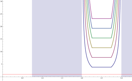
Figure 4: The set $\mathcal{Z}^{+}_{2}(V_{g}g)$.

When $t\in[0,1/\sqrt{1}5)$ we get the set $\mathcal{Z}^{+}_{1}(V_{g}g)$, which is described by Proposition A.1, as union of two sets. The first one corresponds to the set

$$\Big{(}\frac{1}{\sqrt{1}5}-\frac{k}{\nu}\,,\,\nu\Big{)}$$

where $n,k\in\mathbb{N}$, $\displaystyle\nu=\frac{n}{1-2/\sqrt{1}5}$, and $\displaystyle\frac{k}{\nu}\in(0,\,1/\sqrt{1}5]$.

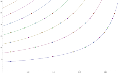
Figure 5: The squares describe the first subset of $\mathcal{Z}^{+}_{1}(V_{g}g)$ in Proposition A.1.

The second one corresponds to the set

$$\Big{(}\frac{k}{n}-\beta,n\Big{)},$$

where $k,n\in\mathbb{N}$ and $\displaystyle\frac{k}{n}\in[\beta,\beta+\alpha)$.

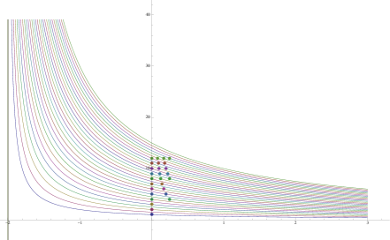
Figure 6: The circles describe the second subset of $\mathcal{Z}^{+}_{1}(V_{g}g)$ in Proposition A.1.

Figure 7 describes completely the set $\mathcal{Z}^{+}(V_{g}g)$.

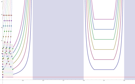
Figure 7: The set $\mathcal{Z}^{+}(V_{g}g)$ corresponding to $\alpha=1/\sqrt{1}5$ and $\beta=2$.

The case $\alpha=1/2$ and $\displaystyle\beta\in\frac{1}{2}\mathbb{N}$

As in the case $\alpha<1$, the description of $\mathcal{Z}^{+}_{2}(V_{g}g)$ is much simpler. Indeed, as a direct consequence of Lemma 4.10 we get that

$$\mathcal{Z}^{+}_{2}(V_{g}g)=\begin{cases}(t,\nu)&\mbox{$t\in[1/2,\beta]\cup[\beta+1,\infty),\nu>0$ }\\ (t,{k}/{(t-\beta)})&\mbox{$t\in(\beta,\beta+1/2),k\in\mathbb{N}$}\\ (t,k/(\beta+1-t))&\mbox{$t\in[\beta+1/2,\beta+1),k\in\mathbb{N}$}.\\ \end{cases}$$

On the other hand, the description of $\mathcal{Z}^{+}_{1}(V_{g}g)$ is given in the following proposition.

Proposition A.2.

Let $\Omega=[0,1/2)\cup[1/2+\beta,1+\beta)$, and $g=\chi_{\Omega}$. Then if $t\in[0,1/2]$

$$\mathcal{Z}^{+}_{1}(V_{g}g)=\begin{cases}\displaystyle\Big{(}t,\frac{k}{1/2-t}\Big{)}&\mbox{$t\in[0,1/2]$, and $k\in\mathbb{N}$}\\ \ &\\ \displaystyle\Big{(}\frac{k}{\nu}-\beta\,,\,\nu\Big{)}&\mbox{$k\in\mathbb{N}$, $\displaystyle\nu=\frac{n}{2\beta+1}$, and $\displaystyle\frac{k}{n}\in\Big{[}\frac{\beta}{2\beta+1},\,\frac{1}{2}\Big{]}$}\\ \ &\\ \displaystyle\Big{(}t,\frac{2k}{2\beta+1}\Big{)}&\mbox{$k\in\mathbb{N}$ and $t\in[0,1/2]$}.\\ \end{cases}$$

Proof.

Recall that in (13) we have

$$\Omega\cap(\Omega+t)=\begin{cases}[t,1/2]\cup[\beta+1/2+t,\beta+1]&\mbox{if $t\in[0,1/2)$}\\ [\beta+1/2,t+1/2]&\mbox{if $t\in[\beta,\beta+1/2)$}\\ [t,\beta+1]&\mbox{if $t\in[\beta+1/2,\beta+1)$}.\end{cases}$$ (21)

Then, a direct computation shows that $V_{g}g(t,\nu)=0$ and $t\in[0,1/2]$ we have that the following system should be satisfied:

$$e^{-2\pi i\nu t}-e^{-\pi i\nu}+e^{-2\pi i\nu(\beta+1/2+t)}-e^{-2\pi i\nu(\beta+1)}=0$$

Since, for given $z_{i},$ so that $|z_{i}|=1$ for every $i=1,2,3,4$, all solutions to $z_{1}+z_{2}+z_{3}+z_{4}=0$ are given by any pairs of opposite numbers and so we have the following cases:

• $e^{-2\pi i\nu t}=e^{-\pi i\nu}$ and $e^{-2\pi i\nu(\beta+1/2+t)}=e^{-2\pi i\nu(\beta+1)}$;

• $e^{-2\pi i\nu t}=e^{-2\pi i\nu(\beta+1)}$ and $e^{-\pi i\nu}=e^{-2\pi i\nu(\beta+1/2+t)}$;

• $-e^{-2\pi i\nu t}=e^{-2\pi i\nu(\beta+1/2+t)}$ and $-e^{-\pi i\nu}=e^{-2\pi i\nu(\beta+1)}$.

Case (i):

In this case we have that for $t\in[0,1/2]$

$$\nu(1/2-t)=k,$$

where $k\in\mathbb{N}$.

Case (ii):

In this case

$$\nu(t-\beta-1)\in\mathbb{N}\quad\text{ and }\quad\nu(t+\beta)\in\mathbb{N},$$

where $k,m\in\mathbb{N}$. This yields

$$\nu(\beta+t)=k\quad\text{ and }\quad\nu(2\beta+1)=n.$$

So $\displaystyle t=\frac{k}{\nu}-\beta$ and $\displaystyle\nu=\frac{n}{2\beta+1}$. Since $t\in[0,1/2)$ we have that $\displaystyle\frac{k}{n}\in\Big{[}\frac{\beta}{2\beta+1},\,\frac{1}{2}\Big{]}$.

Case (iii):

Finally, we get that

$$2\nu(\beta+1/2)=2k+1$$

where $k\in\mathbb{N}\cup\{0\}$.

$\blacksquare$

Example

Let $\alpha=1/2$ and $\beta=2$. The next picture corresponds to $\mathcal{Z}^{+}_{2}(V_{g}g)$

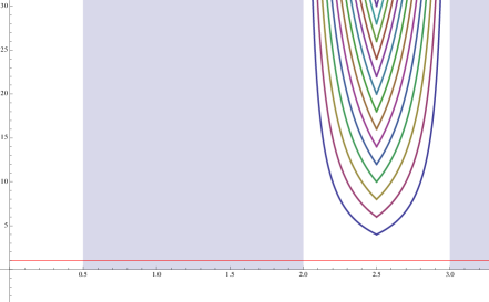
Figure 8: The set $\mathcal{Z}^{+}_{2}(V_{g}g)$.

The set $\mathcal{Z}^{+}_{1}(V_{g}g)$, is given as union of three sets as calculated by Proposition A.2. Any of this set is described by figures 9, 10 and 11.

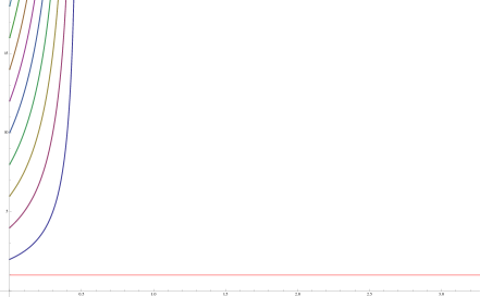
Figure 9: The hyperbolas describe the first subset of $\mathcal{Z}^{+}_{1}(V_{g}g)$ in Proposition A.2.

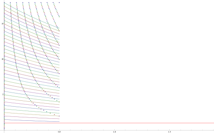
Figure 10: The dots describe the second subset of $\mathcal{Z}^{+}_{1}(V_{g}g)$ in Proposition A.2.

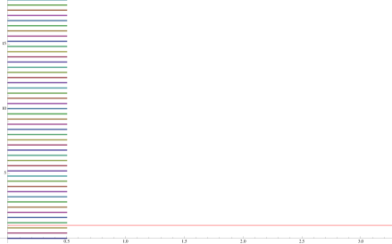
Figure 11: The lines describe the third subset of $\mathcal{Z}^{+}_{1}(V_{g}g)$ in Proposition A.2.

Finally the set $\mathcal{Z}^{+}(V_{g}g)$ is given in Picture 12.

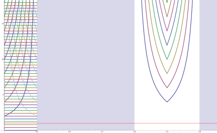
Figure 12: The set $\mathcal{Z}^{+}(V_{g}g)$ corresponding to the case $\alpha=1/2$ and $\beta=2$.

Elona Agora, Instituto Argentino de Matemática “Alberto P. Calderón” (IAM-CONICET), Buenos Aires, Argentina
E-mail address: elona.agora@gmail.com

Jorge Antezana, Departamento de Matemática, Universidad Nacional de La Plata and, Instituto Argentino de Matemática “Alberto P. Calderón” (IAM-CONICET), Buenos Aires, Argentina
E-mail address: antezana@mate.unlp.edu.ar

Mihail N. Kolountzakis, Department of Mathematics and Applied Mathematics University of Crete, Heraklion, Greece
E-mail address: kolount@gmail.com

References

- [1]
- [2] B. Fuglede, Commuting self-adjoint partial differential operators and a group theoretic problem J. Func. Anal. 16 (1974), 101-121.
- [3] I. aba, Fuglede’s conjecture for a union of two intervals Prodeedings of the AMS, Vol. 129, no. 10 (2001), 2965-2972.
- [4] Y.M. Liu and Y. Wang, The uniformity of non-uniform Gabor bases Adv. Comput. Math., 18 (2003), 345-355.
- [5] J.P. Gabardo, C.K. Lai, Y. Wang, Gabor orthonormal bases generated by the unit cube J. Func. Anal. 269, no. 5 (2014).
- [6] D. Gabor, Theory of communication J. Inst. Elec. Eng. (London), 93 (1946), 429-457
- [7] K. Gröchenig, Foundations of time-frequency analysis Applied and Numerical Harmonic Analysis. Birkhäuser Boston, Inc., Boston, MA, 2001. xvi+359 pp.
- [8] M. Kolountzakis, Packing, tiling, orthogonality and completeness Bull. London Math. Soc. 32 (2000), 5, 589-599.
- [9] M. Kolountzakis, The study of translational tiling with Fourier Analysis In L. Brandolini, editor, Fourier Analysis and Convexity, pages 131-187. Birkhäuser, 2004.