Ion-scale turbulence in MAST: anomalous transport, subcritical transitions, and comparison to BES measurements

Abstract

We investigate the effect of varying the ion temperature gradient (ITG) and toroidal equilibrium scale sheared flow on ion-scale turbulence in the outer core of MAST by means of local gyrokinetic simulations. We show that nonlinear simulations reproduce the experimental ion heat flux and that the experimentally measured values of the ITG and the flow shear lie close to the turbulence threshold. We demonstrate that the system is subcritical in the presence of flow shear, i.e., the system is formally stable to small perturbations, but transitions to a turbulent state given a large enough initial perturbation. We propose that the transition to subcritical turbulence occurs via an intermediate state dominated by low number of coherent long-lived structures, close to threshold, which increase in number as the system is taken away from the threshold into the more strongly turbulent regime, until they fill the domain and a more conventional turbulence emerges. We show that the properties of turbulence are effectively functions of the distance to threshold, as quantified by the ion heat flux. We make quantitative comparisons of correlation lengths, times, and amplitudes between our simulations and experimental measurements using the MAST BES diagnostic. We find reasonable agreement of the correlation properties, most notably of the correlation time, for which significant discrepancies were found in previous numerical studies of MAST turbulence.

1 Introduction

Understanding and controlling turbulence is crucial to the realisation of fusion as an energy source [1]. Turbulence at perpendicular length scales of the order of the ion Larmor radius can be driven by: the ion temperature gradient (ITG) $\kappa_{T}\equiv-\derivative*{\ln T_{i}}{r}$ ($T_{i}$ is the ion temperature and $r$ is a dimensionless radial coordinate defined later), which drives the well-known ITG instability [2, 3]; the electron temperature gradient (ETG) $\kappa_{Te}\equiv-\derivative*{\ln T_{e}}{r}$ (where $T_{e}$ is the electron temperature), which at sufficient $\beta$ (ratio of plasma pressure to magnetic pressure) can drive microtearing modes (MTMs) [4]; and a combination of electron temperature and density gradients, which drive trapped-electron modes (TEMs) [5]. The electron temperature gradient also drives ETG modes that create plasma turbulence at finer electron scales [6, 7]. Recent experimental [8, 9] and numerical [10] studies of JET plasmas have demonstrated that ion-scale turbulence is “stiff” with respect to changes in $\kappa_{T}$, i.e., small changes in $\kappa_{T}$ can lead to large changes in the turbulent transport. Similarly, there is experimental evidence that small-scale electron turbulence exhibits similar behaviour due to changes in $\kappa_{Te}$ [11]. Power-balance calculations for the Mega Ampere Spherical Tokamak (MAST) indicate that heat transport is usually carried predominantly through the electron channel [12], and gyrokinetic simulations have shown that it can be due to a combination of microtearing modes, which have been shown to be unstable at $\beta\gtrsim 0.1$, and fine-scale ETG-driven turbulence [13, 14, 15, 4, 16, 17]. Similar findings have also been reported for NSTX [18, 19, 20, 21, 22, 23]. The main reason for the dominance of the electron channel and relative weakness of the ion transport is believed to be the suppression of ion-scale turbulence by significant differential rotation present in spherical tokamaks. Understanding, based on measuring and modelling the structure of this weak ion-scale turbulence, the physics of the associated transport and of its suppression is a key challenge of fusion plasma theory, both for MAST and for tokamaks generally.

Indeed, studies of many experiments have shown that turbulence can be affected by the profile of the toroidal rotation, which is driven by the neutral beam injection (NBI) heating system [24, 8, 9, 25, 26]. The plasma flow associated with toroidal rotation, which is sheared, has components both parallel and perpendicular to the direction of the magnetic field. Perpendicular flow shear, quantified by $\gamma_{E}=(r/q)\derivative*{\omega}{r}$ $(a/v_{\mathrm{th}i})$ ($q$ is the safety factor, $\omega$ is the frequency of toroidal rotation, $a$ is the minor radius of the device, $v_{\mathrm{th}i}=\sqrt{2T_{i}/m_{i}}$ is the thermal velocity, and $m_{i}$ is the ion mass), has been shown to reduce, or even eliminate, turbulence in tokamaks [24, 27]. Numerical studies of core turbulence in MAST [12, 28, 25] and NSTX [29, 30] have confirmed that ion-scale turbulence is often suppressed by the perpendicular flow shear. Parallel flow shear has also been shown to drive a linear instability [31], which can increase the level of turbulence, although, at the levels of flow shear considered in this work, we do not expect the destabilising effect of the parallel flow shear to be significant. Thus, at ion scales, there is a competition in fusion plasmas between the destabilising effects of the ITG/TEM instabilities and the parallel flow shear, and the stabilising effect of the perpendicular flow shear.

It has been shown that perpendicular flow shear can render the plasma completely linearly stable [32]. However, this may still entail substantial transient growth of perturbations and, given a large enough initial perturbation, can lead to a saturated nonlinear state – a phenomenon known as “subcritical” turbulence [28, 33, 34, 35, 36]. We have previously studied this transition to subcritical turbulence in MAST in Ref. [37], and proposed the following transition scenario: close to the turbulence threshold, the nonlinear state is dominated by coherent, long-lived structures; as the system is taken away from the threshold, the number of these structures increases until they fill the simulation domain and a conventional turbulent state is recovered. In this paper, we will focus on the nature of ion-scale turbulence in MAST (driven by a combination of the ITG and trapped electron modes) and present a more comprehensive view of the changes in turbulence that occur as the system is taken away from the threshold. We do this via nonlinear gyrokinetic simulations by varying $\kappa_{T}$ and $\gamma_{E}$ and perform an analysis of the turbulence structure and make detailed comparisons with experimental measurements.

At the temperatures and densities found in fusion experiments such as MAST, it can be shown that the conditions for a fluid description are rarely satisfied and that a kinetic description must be used. Gyrokinetics [38, 39, 40] has emerged as the most appropriate first-principles description in the context of plasma turbulence in the core of tokamaks. In this paper, we use the local gyrokinetic code GS2 [41, 6] to solve the gyrokinetic equation. GS2 includes a large number of physical effects relevant to experimental plasmas, such as realistic magnetic-surface geometries, arbitrary numbers of kinetic species, realistic Fokker-Planck collision operators, and so on. This has allowed simulations of sufficient realism to be compared quantitatively to experimental measurements. Local gyrokinetic codes, such as GS2, take as input the values and first derivatives of equilibrium quantities at a particular radial location and predict a host of quantities that could theoretically be measured by an experimental diagnostic, for example, the flux of particles, momentum, and heat, or, indeed, the full density and temperature fluctuation fields.

In conjunction with increasingly realistic modelling, more sophisticated diagnostic techniques have been developed, which aid in our understanding of the conditions inside the reactor and allow us to make comparisons with modelling results. The beam-emission-spectroscopy (BES) diagnostic in MAST is one such diagnostic that measures ion-scale density fluctuations [42, 43]. More specifically, the BES diagnostic infers ion-scale density fluctuations from D_α emission (the emission of light resulting from the dominant (n=3-2) visible transition of ionised deuterium), which is generated as a result of the injection of neutral particles by the NBI system. The BES diagnostic takes measurements in a two-dimensional radial-poloidal plane. From the BES measurements, it is possible to estimate a number of useful correlation properties of the turbulence [44, 45, 46, 47, 48, 49]: the correlation time $\tau_{c}$, via the cross-correlation time delay (CCTD) method; the radial and poloidal correlation lengths $l_{R}$ and $l_{Z}$; and the relative density-fluctuation field $\delta n_{i}/n_{i}$. Measurements of fluctuating quantities allow more extensive quantitative comparisons between experiment and simulations via the use of “synthetic diagnostics”, which take account of the measurement characteristics of the particular diagnostic and modify the simulation output accordingly [50, 47, 51, 49].

Previous studies of BES data and comparisons with ion-scale simulation data have been performed on DIII-D [52, 45, 50, 53, 54, 46, 55] and MAST [51]. In the L-mode studies on DIII-D, good agreement was found between experimental measurements and synthetic results from local simulations in the mid-core region ($0.4<r/a<0.75$, where $r/a$ is the normalized radius), both in terms of transport and fluctuation characteristics. In the outer-core region ($r/a>0.75$), GYRO simulations again showed good agreement for the fluctuation characteristics, but underpredicted the heat fluxes and fluctuation amplitudes by almost an order of magnitude [50, 53, 54, 46]. However, subsequent local simulations using the GENE code [55] more closely matched the experimental measurements. The motivation for this work is the study performed in Ref. [51] of MAST turbulence that used the BES diagnostic to measure turbulent density fluctuations in the outer core of an L-mode plasma and compared their correlation properties with those inferred from global gyrokinetic simulations. The discharge studied was specifically designed to have high flow shear at mid-radius to produce an internal transport barrier (ITB), and, as a consequence, had low flow shear in the outer core, where ion-scale turbulence would not, therefore be completely suppressed. There was some agreement at mid-radii, however, significant discrepancies were found in the ion heat flux and turbulence correlation time at outer radii. In this work we simulate ion-scale turbulence in the outer core of the same L-mode discharge as in [51] using high-resolution local gyrokinetic simulations. While previous gyrokinetic modelling of similar MAST L-mode plasmas showed that electron-scale turbulence can play a significant role [28, 25] (as is the case for this discharge, where $Q_{e}\sim 8Q_{i}$), it has been shown that the suppression of ion heat transport is due to the effect of flow shear and it is this phenomenon that we study further in this paper. Therefore, it is of interest to study purely ion-scale turbulence, as we do in this work, in order to make comparisons with BES data, which only covers turbulent fluctuations at ion scales. We shall see that local gyrokinetic modelling does produce turbulent fluctuations whose correlation properties are consistent with experimental measurements, in particular the turbulence correlation time. However, we also find that GS2 underpredicts the turbulence amplitude, similar to previous studies [50, 53, 46, 55].

In simulating experimentally relevant plasmas using gyrokinetic codes, we aim to achieve the following. First, we want to understand better the physical mechanisms that most strongly influence turbulence and the associated enhanced transport. Specifically, we wish to know how turbulence characteristics (such as transport, spatial scales, time scales, etc.) change in the outer core of MAST with the equilibrium parameters $\kappa_{T}$ and $\gamma_{E}$. Secondly, in light of newly available experimental data from the MAST BES diagnostic [51], we want to establish whether the turbulence characteristics found in local gyrokinetic GS2 simulations agree with experimental BES measurements within the experimental uncertainties in measurements of $\kappa_{T}$ and $\gamma_{E}$. Such quantitative comparisons with experimental results are essential in developing confidence in our theoretical models and numerical implementations. In understanding the properties of turbulence, we ultimately aim to guide the optimisation and design of future experiments and fusion reactors by acquiring the ability to predict and control the turbulence.

The rest of this paper is organised as follows. In section 2, we give an overview of the MAST discharge that we will be considering, as well as of gyrokinetics and of the numerical tools that we will use for our study. Our main results are split into two sections.

In section 3, we study numerically the effect on turbulence in MAST of changing $\kappa_{T}$ and $\gamma_{E}$ by performing a two-dimensional parameter scan in these two equilibrium parameters. We map out the turbulence threshold and show that the experimentally measured ion heat flux is close to the numerical values found near this threshold, thus suggesting that the turbulence in MAST is near-marginal (section 3.1). We demonstrate that the turbulence is subcritical (section 3.2), with large initial perturbations required to ignite it (a phenomenon not previously observed for an experimentally relevant plasma) and estimate the conditions necessary for the onset of turbulence. We then show that the near-threshold state is one dominated by long-lived, coherent structures, which exist against a background of much smaller fluctuations (section 3.3). These structures are shown to be regions of increased density, radial flow, and temperature fluctuations. Sufficiently far from the turbulence threshold in parameter space, we recover a more conventional turbulent state consisting of many strongly interacting eddies while being sheared apart by the perpendicular flow shear. We demonstrate that many of the properties of the system (e.g. the number of structures, their amplitude, shear due to zonal flows, etc.) are effectively functions only of the distance from the turbulence threshold, as quantified by the ion heat flux.

In section 4, we make comparisons with experimental measurements from the BES diagnostic. We present two types of correlation analysis of our simulations: of the numerical data processed through a synthetic diagnostic (section 4.3) and of raw GS2 data, with no modelling of the diagnostic (section 4.4). We show that there is reasonable agreement with experimental measurements in the case of the analysis with the synthetic diagnostic. However, radial correlation lengths predicted by GS2 are shown to be below the resolution threshold of the BES diagnostic in MAST (an issue discussed in detail in [49]). This conclusion stems from studying correlation parameters of the raw GS2 density fluctuations and suggests that care must be taken when interpreting BES measurements. Comparison between results of analysis with and without the synthetic diagnostic shows that the synthetic diagnostic has a measurable effect on several turbulence characteristics, including the poloidal correlation length and the fluctuation amplitude, consistent with the conclusions of Ref. [49]. Finally, we present the correlation lengths and times as functions of the ion heat flux and again show that the structure of the turbulence in our simulations is effectively only a function of this parameter, which measures the distance to the turbulence threshold.

2 Experimental and numerical details

2.1 MAST discharge #27274

MAST is a medium-sized, low-aspect-ratio ($\approx 1.5$) tokamak with a major radius $R_{0}\approx 0.9$ m and a minor radius $a\approx 0.6$ m. In this work, we will focus on the MAST discharge #27274, one of a set of three nominally identical experiments (i.e. having identical profiles and equilibria) previously reported in [51] and differing only in the radial viewing location of the BES system. These three discharges were #27272, #27268, and #27274, wherein the centre of the BES was located at $1.05$ m, $1.2$ m, and $1.35$ m, respectively. The MAST BES diagnostic [42, 43] observes an area of approximately $16\times 8$ cm² in the radial and poloidal directions, respectively, corresponding approximately to one third of the minor radius of the plasma. Thus, the combination of these three discharges provided a complete radial profile of BES measurements on the outboard side of the plasma.

Each discharge produced an L-mode plasma with strong toroidal rotation and, therefore, with mean flow shear perpendicular and parallel to the magnetic field [51]. Previous investigations of MAST turbulence for similar configurations [28, 25] found that ion-scale turbulence is suppressed in the core region by strong flow shear. However, the flow shear is weaker in the outer-core region, where ITG modes are not completely suppressed, making it possible to study ion-scale turbulence. In this work, we will restrict our attention to the time window $t=0.250\pm 0.002$ s and the radial location $r=D/2a=0.8~{}(\equiv r_{0})$ of discharge #27274, where $D$ is the diameter of the flux surface and $a$ is the half diameter of the last closed flux surface (LCFS), both measured at the height of the magnetic axis. Importantly, there is no large-scale and disruptive magnetohydrodynamic (MHD) activity at this time and radial location [51]; such activity would interfere with the quality of BES measurements. The normalized radial location $r=0.8$ corresponds to a major radius of approximately $1.32$ m and, therefore, falls within the viewing area covered by discharge #27274 [see figure 1(b)].

2.2 Equilibrium profiles

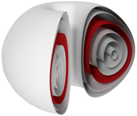
(a)

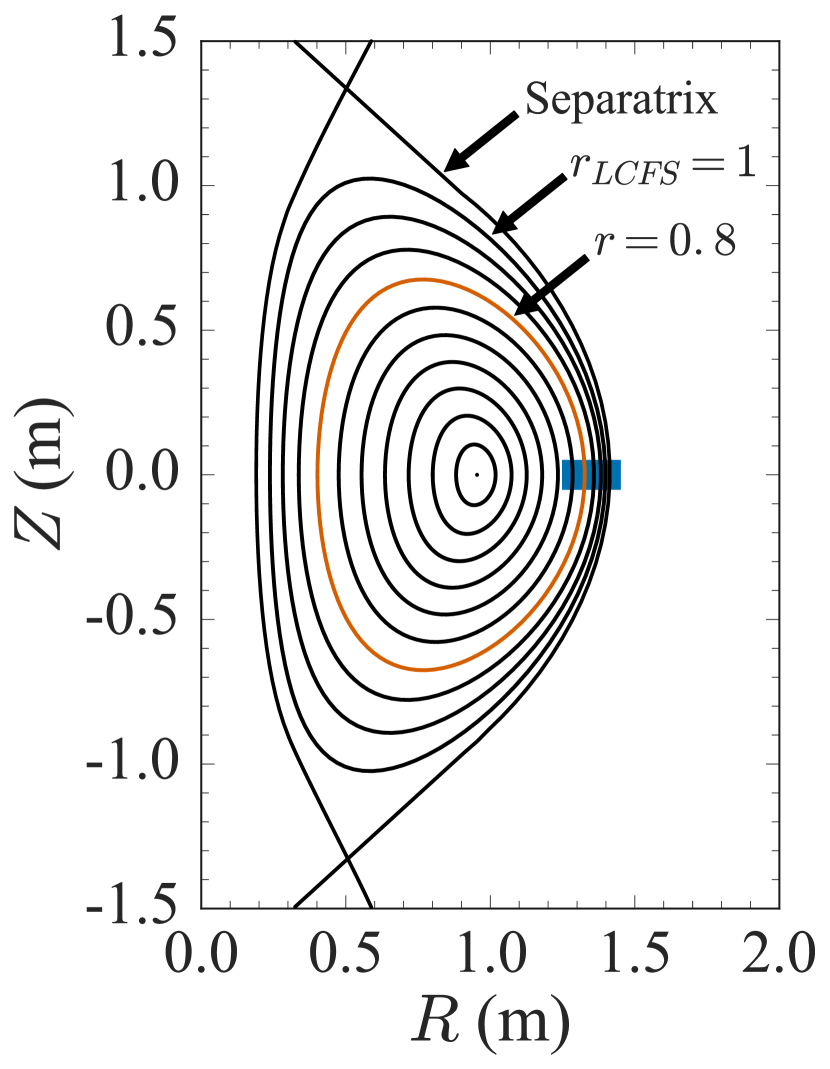
(b)

Figure 1: 1(a) A three-dimensional view of the nested flux surfaces. 1(b) The poloidal cross-section of the magnetic geometry along with the LCFS and the separatrix, which separates closed field lines from open ones. The flux surface of interest is at $r=0.8$, shown in red. It was chosen so that this surface intersects the BES measurement plane for discharge #27274 (blue shaded region).

MAST has a range of diagnostics that allow us to extract the equilibrium parameters required to conduct a numerical transport study. The ion temperature, $T_{i}$, and toroidal flow velocity, $u_{\phi}=R\omega$, where $\omega$ is the toroidal angular rotation frequency, were obtained from charge-exchange-recombination spectroscopy (CXRS) measurements of C⁺⁶ impurity ions with a spatial resolution of $\sim 1$ cm [57]. The electron density, $n_{e}$, and temperature, $T_{e}$, were obtained from a Thomson-scattering diagnostic [58] with resolution comparable to the CXRS system. These measured profiles were mapped onto flux-surface coordinates by the pre-processing code $MC^{\mathit{3}}$ using a motional-Stark-effect-constrained EFIT equilibrium [59]. These equilibrium profiles served as input to the transport analysis code TRANSP [60], which calculates the transport coefficients of particles, momentum, and heat. Figure 1(a) shows a three-dimensional view of the axisymmetric nested flux surfaces and figure 1(b) shows the poloidal cross-section of the flux surfaces extracted from an EFIT equilibrium. The $r=0.8$ surface is highlighted in both plots. The measurement window of the BES diagnostic for discharge #27274 is also shown in figure 1(b). The chosen flux surface at $r=0.8$ intersects the measurement window at the outboard midplane, allowing comparisons of turbulence characteristics between our numerical predictions of turbulence and experimental measurements.

The important experimental quantities needed to conduct a numerical study are the radial profiles of $T_{i}$, $T_{e}$, $n_{i}$ (the ion density), $n_{e}$, and $\omega$. There are no direct measurements of $n_{i}$ in MAST, but we assume that it is equal to $n_{e}$, as measured by the Thomson-scattering diagnostic, due to quasineutrality (in MAST, we typically have an effective ion charge $Z_{\mathrm{eff}}\lesssim 1.5$). To conduct a numerical study of turbulence at $r=0.8$ (using the local formulation of gyrokinetics; see section 2.3), we need the equilibrium quantities listed above and their first derivatives (gradient length scales). The (normalised) gradient length scales of $T_{i}$, $T_{e}$, and $n_{e}$, and flow shear (gradient of $\omega$) are, by definition,

$$\frac{1}{L_{Ti}} =-\derivative{\ln T_{i}}{r}\equiv\kappa_{T},$$ (1)

$$\frac{1}{L_{Te}} =-\derivative{\ln T_{e}}{r},$$ (2)

$$\frac{1}{L_{ne}} =-\derivative{\ln n_{e}}{r},$$ (3)

$$\mathrm{and}\hskip 20.00003pt\gamma_{E} =\frac{r_{0}}{q_{0}}\derivative{\omega}{r}\frac{a}{v_{\mathrm{th}i}},$$ (4)

where $q(\psi)=\partialderivative*{\psi_{\mathrm{tor}}}{\psi_{\mathrm{pol}}}$ is the safety factor and $q_{0}$ is its value at $r_{0}$. The flow-shear parameter $\gamma_{E}$ can be interpreted as the (non-dimensionalised) shear of the component of the toroidal rotation that is perpendicular to the local magnetic field.

The left-hand column of figure 2 shows the radial profiles of $T_{i}$, $T_{e}$, $n_{e}$, and $\omega$ as functions of $r$. The gradient scale lengths (1)–(3) and flow shear (4) are plotted as functions of $r$ in the right-hand column in figure 2. The dashed lines indicate $r=0.8$. The profiles in figure 2 (and in figure 3 below) represent a $20$-ms time average around $t=0.25$ s and the shaded areas indicate the standard deviations. The nominal experimental values of the quantities that we will vary in this study are $\kappa_{T}=5.1\pm 1$ and $\gamma_{E}=0.16\pm 0.02$.

The profiles of the ion and electron heat fluxes ($Q_{i}^{\exp}$ and $Q_{e}^{\exp}$, respectively) were obtained from a transport analysis using TRANSP based on the equilibrium profiles shown in figure 2. The profiles are shown in figure 3. In this work, we normalise all heat fluxes to the ion gyro-Bohm value

$$Q_{\mathrm{gB}}=n_{i}T_{i}v_{\mathrm{th}i}\frac{\rho_{i}^{2}}{a^{2}},$$ (5)

where $\rho_{i}$ is the ion gyroradius. We see from figure 3 that the main loss of heat in the system is via transport due to the electrons: the experimental level of ion heat flux at $r=0.8$ is $Q^{\exp}_{i}/Q_{\mathrm{gB}}=2\pm 1$, while the electron heat flux is $Q^{\exp}_{e}/Q_{\mathrm{gB}}=15.2\pm 0.9$. This is partially due to the suppression of ion turbulence by flow shear (as we will show in this paper) and possibly also due to significant heat transport driven in the electron channel via the ETG instability and MTMs as has been observed in other studies [13, 14, 28, 21, 22, 16]. In this work, we will focus exclusively on ion-scale turbulence in order to make contact with ion-scale turbulence measurements from the BES. We will briefly comment on the transport predicted by our simulations in the electron channel, but leave the full investigation to future work.

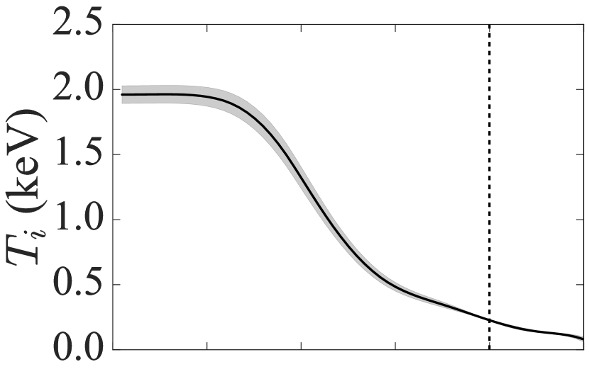
(a)

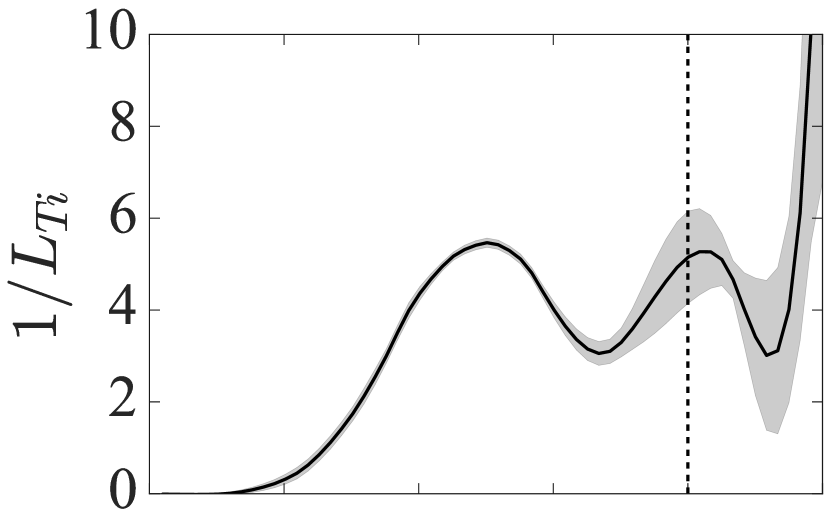
(b)

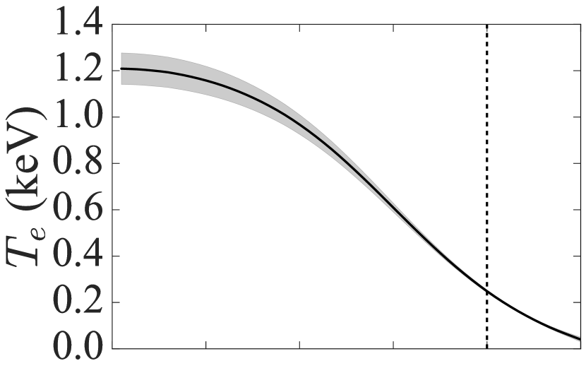
(c)

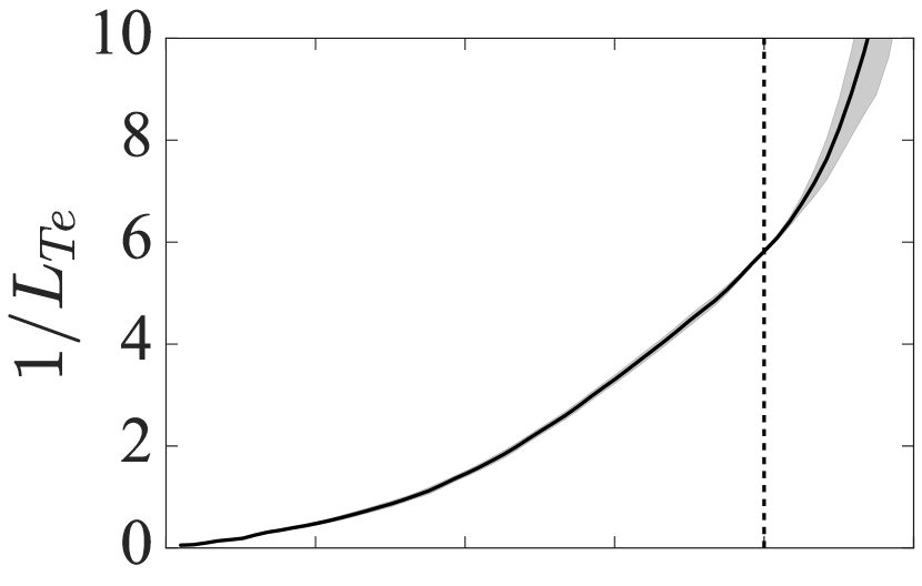
(d)

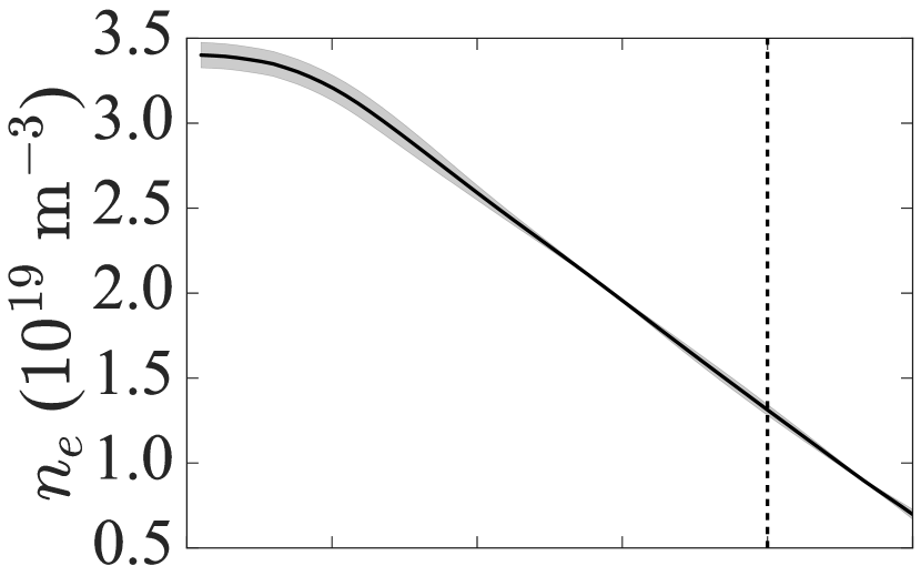
(e)

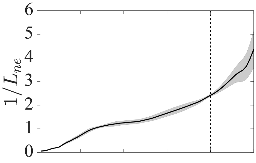
(f)

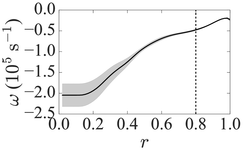
(g)

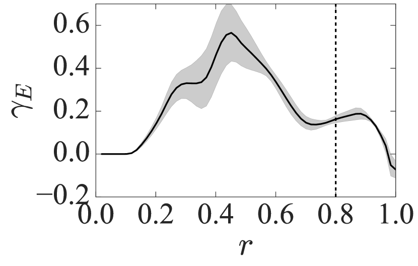
(h)

Figure 2: Radial profile measurements from MAST discharge #27274 of 2(a) the ion temperature, $T_{i}$, 2(b) the ion temperature gradient, $1/L_{Ti}$, calculated using (1), 2(c) the electron temperature, $T_{e}$, 2(d) the electron temperature gradient, $1/L_{Te}$, calculated using (2), 2(e) the electron density, $n_{e}$, 2(f) the electron density gradient, $1/L_{ne}$, calculated using (3), 2(g) the toroidal angular frequency, $\omega$, and 2(h) the flow shear, $\gamma_{E}$, calculated using (4). The dashed line in each plot indicates $r=0.8$ and the shaded regions indicate the standard deviation of the profiles over a $20$-ms time window around $t=0.25$ s.

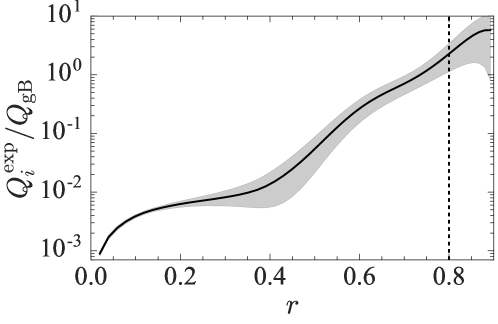
Figure 3: Experimental ion and electron heat fluxes as functions of $r$ determined from power balance by TRANSP analysis. Both fluxes are normalized to the local ion gyro-Bohm value (5). The dashed line indicates $r=0.8$, where BES measurements were made, and the shaded regions indicate the uncertainty estimated by TRANSP.

2.3 Local gyrokinetic description

We model the turbulence in MAST using gyrokinetic theory [38, 39, 40]. For a detailed review, the reader is referred to [40] and references therein, while only a brief overview is given here. The gyrokinetic equation describes the evolution of the non-Boltzmann part of the perturbed (from a background Maxwellian $F_{s}$) particle distribution function, $h_{s}(t,{\bf\it R}_{s},\varepsilon_{s},\mu_{s},\sigma)$, of a species $s$, where ${\bf\it R}_{s}$ is the guiding-centre coordinate, $\varepsilon_{s}$ is the particle energy, $\mu_{s}$ is the magnetic moment of species $s$, and $\sigma$ is the sign of the (peculiar) parallel velocity $v_{\parallel}$. The gyrokinetic equation is

$$\begin{split}&\left(\partialderivative{t}+{\bf\it u}\cdot\nabla\right)\left(h_{s}-\frac{Z_{s}e\left<{\varphi}\right>_{{\bf\it R}_{s}}}{T_{s}}F_{s}\right)+\left(v_{\parallel}{\bf\it b}+{\bf\it V\!}_{{\rm D}s}+\left<{{\bf\it V\!}_{E}}\right>_{{\bf\it R}_{s}}\right)\cdot\nabla{h_{s}}-\left<{C[h_{s}]}\right>_{{\bf\it R}_{s}}\\ &\quad=-\left<{{\bf\it V\!}_{E}}\right>_{{\bf\it R}_{s}}\cdot\nabla r\left[\derivative{\ln n_{s}}{r}+\left(\frac{\varepsilon_{s}}{T_{s}}-\frac{3}{2}\right)\derivative{\ln T_{s}}{r}+\frac{m_{s}v_{\parallel}}{T_{s}}\frac{RB_{\phi}}{B}\derivative{\omega}{r}\right]F_{s},\end{split}$$ (6)

where ${\bf\it u}=\omega(r)R^{2}\nabla\phi$ is the toroidal rotation velocity, $\omega(r)$ is the toroidal angular frequency, $\phi$ is the toroidal angle, $\varphi$ is the electrostatic potential perturbation, $\left<{\ldots}\right>_{{\bf\it R}_{s}}$ is an average over the particle orbit at constant ${\bf\it R}_{s}$, $F_{s}=n_{s}(r){\left[m_{s}/2\pi T_{s}(r)\right]}^{3/2}e^{-\varepsilon_{s}/T_{s}(r)}$ is the background Maxwellian, ${\bf\it V\!}_{{\rm D}s}=(c/Z_{s}eB){\bf\it b}\times\left[m_{s}v_{\parallel}^{2}{\bf\it b}\cdot\nabla{\bf\it b}+\mu\nabla B\right]$ is the magnetic drift velocity,

$${\bf\it V\!}_{E}=\frac{c}{B}{\bf\it b}\times\nabla\varphi$$ (7)

is the ${\bf\it E}\times{\bf\it B}$ drift velocity, $C[h_{s}]$ is the linearised collision operator [61, 62], and $B_{\phi}$ is the toroidal component of the magnetic field.

To close our system of equations we use the quasineutrality condition

$$\sum_{s}Z_{s}\delta n_{s}=0\quad\Rightarrow\quad\sum_{s}\frac{Z_{s}^{2}e\varphi}{T_{s}}n_{s}=\sum_{s}Z_{s}\int d^{3}{\bf\it v}\left<{h_{s}}\right>_{{\bf\it r}},$$ (8)

where $\left<{\ldots}\right>_{{\bf\it r}}$ indicates a gyroaverage at constant particle position ${\bf\it r}$, to calculate $\varphi$ using $h_{s}$.

In order for the local approximation to be valid, we require that $\rho_{i}/a\ll 1$, where we assume that other important length scales in the system, such as $L_{Ti}$, are of the same order as $a$. The turbulence predicted by our simulations is, therefore, only representative of the turbulence at a single flux surface, even though our box sizes can be the size of MAST (several such formally overlapping simulations can be then used to model transport across the entire radial extent of the machine). For the MAST discharge and radial location studied in this work, one finds $\rho_{i}/a\sim 1/100$, where $\rho_{i}\approx 6\times 10^{-3}$ m and $a\approx 0.6$ m. While this is a reasonably small number, previous studies of simpler geometries have suggested that non-local effects can reduce the level of turbulent transport by 50% at values similar to $1/100$ [63, 64]. A scan of different values of $\rho^{*}$ using a global gyrokinetic code would be required to test whether non-local effects change the level of turbulence for the MAST turbulence studied in this paper. In addition, the coherent structures described in section 3.3.1 are similar in size to the gradient length scales and so global effects might affect their characteristics. However, the cost of using global simulations would be too large for the parameter scans performed in this paper. There is ongoing work to extend the GS2 code to include finite system-size effects [65], such as profile variation, which may be used in future to test their effect on MAST turbulence.

In adopting equations (6) and (8) we have formally assumed that the Mach number $M$ of the plasma rotation is small, but that the flow shear is large enough to affect the plasma dynamics:

$$\frac{R\omega}{v_{{\mathrm{th}}i}}=M\ll 1,\quad|a\nabla\ln\omega|\sim\frac{1}{M}.$$ (9)

This allows us to formulate local gyrokinetics in a rotating surface, neglecting effects such as the Coriolis and centrifugal force, but retaining the effect of flow shear [40]. We have also assumed that the fluctuations are purely electrostatic, i.e., that there are no fluctuating magnetic fields. Previous studies of MAST [15, 4, 13, 16] and of NSTX [18, 19, 20, 21, 22, 23] have shown that including electromagnetic fluctuations affects core turbulence in regions of the plasma where $\beta\gtrsim 0.1$ and $\beta\gtrsim 0.05$, for MAST and NSTX, respectively. On the peripheral MAST L-mode surface studied in this paper, $\beta$ is smaller than that level by an order of magnitude, viz. $\beta\approx 0.005$, and so electromagnetic effects are expected to be negligible.

2.4 Numerical set-up

In this work, we have used the local gyrokinetic code GS2 [41, 6, 66] to solve the system of equations (6) and (8) to give us the time evolution of $h_{s}$ and $\varphi$. GS2 solves the gyrokinetic equation in a region known as a “flux tube”, shown in figure 4. The GS2 flux tube follows a central magnetic field line once around in the poloidal direction (represented in figure 4 by the field line highlighted in red).

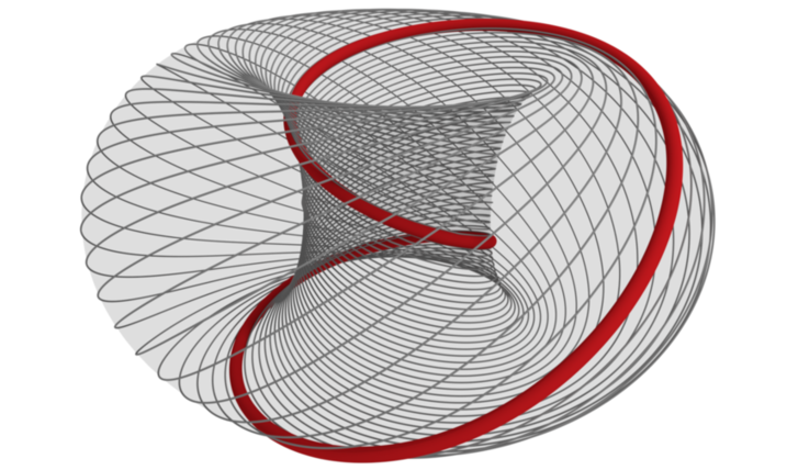
Figure 4: Magnetic field lines that lie on the flux surface at $r=0.8$ (setting $q=2$ for visualisation purposes, so that field lines are closed). The field line marked in red is the centre line of the GS2 flux tube that we use as the simulation domain. The flux tube follows the field line once around the flux surface in the poloidal direction.

The MAST local equilibrium parameters used in our simulations, extracted from the MAST diagnostics and EFIT equilibrium, are given in table 1. We have included electrons in our simulations as a kinetic species. Our GS2 simulations had resolution of $85\times 32\times 20$ grid points in the radial $\times$ binormal $\times$ parallel directions, and $27\times 16$ pitch-angle $\times$ energy-grid points, respectively. The corresponding box sizes were $L_{x}\approx 200\rho_{i}$ in the radial direction (with maximum wavenumber $k_{x,\max}\rho_{i}\simeq 1.3$) and $L_{y}\approx 62\rho_{i}$ in the binormal direction (with maximum wavenumber $k_{y,\max}\rho_{i}\simeq 3$). We note that the radial box size is larger than the minor radius of MAST, however, this is required to achieve sufficient $k_{x}$ resolution to resolve the effect of the flow shear (see appendix D). Artificial numerical dissipation was used to damp electron modes at small scales.

Table 1: GS2 equilibrium parameters calculated from diagnostic measurements and from the EFIT equilibrium of the MAST discharge #27274 and appropriately normalised. The nominal experimental values for $\kappa_{T}$ and $\gamma_{E}$ are $\kappa_{T}=5.1\pm 1$ and $\gamma_{E}=0.16\pm 0.02$. The reference magnetic field is the toroidal magnetic field strength at the magnetic axis, i.e., $B_{\mathrm{ref}}=B_{\phi}(r=0)$.

Quantity	GS2 variable	Value
$\beta={8\pi n_{i}T_{i}}/{B_{\mathrm{ref}}^{2}}$	beta	0.0047
$\beta^{\prime}=\partialderivative*{\beta}{r}$	beta_prime_input	-0.12
Eff. ion charge for collisions $Z_{\mathrm{eff}}={\sum_{i}n_{i}Z_{i}^{2}/|\sum_{i}n_{i}Z_{i}|}$	zeff	1.59
Elec.-ion collisionality $\nu_{ei}$	vnewk_2	0.59
Elec. density $n_{eN}=n_{e}/n_{i}$	dens_2	1.00
Elec. density grad. $1/L_{ne}=-\derivative*{\ln n_{e}}{r}$	fprim_2	2.64
Elec. mass $m_{eN}=m_{e}/m_{i}$	mass_2	$1/(2\times 1836)$
Elec. temp. $T_{eN}=T_{e}/T_{i}$	temp_2	1.09
Elec. temp. grad. $\kappa_{Te}\equiv 1/L_{Te}=-\derivative*{\ln T_{e}}{r}$	tprim_2	5.77
Elongation $\kappa$	akappa	1.46
Elongation derivative $\kappa^{\prime}=\derivative*{\kappa}{r}$	akappri	0.45
Flow shear $\gamma_{E}=(r_{0}/q_{0})\derivative*{\omega}{r}(a/v_{{\mathrm{th}}i})$	g_exb	[0, 0.19]
Ion collisionality $\nu_{i}$	vnewk_1	0.02
Ion density $n_{iN}=n_{i}/n_{i}$	dens_1	1.00
Ion density grad. $1/L_{ni}=-\derivative*{\ln n_{i}}{r}$	fprim_1	2.64
Ion mass $m_{iN}=m_{i}/m_{i}$	mass_1	1.00
Ion temp. $T_{iN}=T_{i}/T_{i}$	temp_1	1.00
Ion temp. grad. $\kappa_{T}\equiv 1/L_{Ti}=-\derivative*{\ln T_{i}}{r}$	tprim_1	[4.3, 8.0]
Magnetic field reference point $R_{\mathrm{geo}}$	r_geo	1.64
Magnetic shear $\hat{s}=r/q\derivative*{q}{r}$	s_hat_input	4.00
Major radius $R_{N}=R/a$	rmaj	1.49
Miller radial coordinate $r={D/2a}$	rhoc	0.80
Safety factor $q=\partialderivative*{\psi_{\mathrm{tor}}}{\psi_{\mathrm{pol}}}$	qinp	2.31
Shafranov Shift $1/a\derivative*{R}{r}$	shift	-0.31
Triangularity $\delta$	tri	0.21
Triangularity derivative $\delta^{\prime}=\derivative*{\delta}{r}$	tripri	0.46

GS2 solves (6) for $h_{s}$, from which one can calculate a range of physical characteristics of the turbulence, e.g., the density-, flow-, temperature-fluctuation fields, as well as particle, momentum, and heat fluxes, and so on. Of particular importance in this work are the ion density fluctuation field,

$$\frac{\delta n_{i}}{n_{i}}=\frac{1}{n_{i}}\int\differential^{3}{\bf\it v}\left<{h_{i}}\right>_{{\bf\it r}},$$ (10)

where $\delta n_{i}/n_{i}$ is an order-unity quantity, and the radially outward, time-averaged turbulent heat flux carried by the ions,

$$Q_{i}=\left\langle\frac{1}{V}\int\differential^{3}{\bf\it r}\int\differential^{3}{\bf\it v}\frac{m_{i}v^{2}}{2}h_{i}{\bf\it V\!}_{E}\cdot\nabla r\right\rangle_{\mathrm{fs}},$$ (11)

where $V$ is the volume of the flux tube and $\langle\ldots\rangle_{\mathrm{fs}}$ denotes a flux-surface average. The heat flux $Q_{i}$ can be normalised to the gyro-Bohm heat flux given by (5).

3 Numerical results

In this section, we present the results of a two-dimensional scan in the two local equilibrium parameters, $\kappa_{T}$ and $\gamma_{E}$, that have been identified to have a strong effect on the properties of the turbulence. We demonstrate that GS2 simulations are able to match the experimental ion heat flux at equilibrium-parameter values within the experimental uncertainty and that the experiment lies close to the turbulence threshold (section 3.1). We find that the turbulence is subcritical, meaning that it can be sustained in the absence of linearly growing eigenmodes: it is driven instead by transiently growing modes, provided the transient growth is sufficient and the initial amplitudes are large enough (section 3.2). We study the linear dynamics and estimate the conditions necessary to ignite turbulence, namely the transient amplification factor and time. Studying the real-space structure of turbulence (section 3.3), we detect coherent, long-lived structures close to marginality, and summarise a novel structure-counting analysis of these previously presented in [37]. Moving away from the turbulence threshold into more strongly-driven regimes, the number of turbulent structures increases rapidly. Far from the turbulence threshold, the turbulence is similar to what is encountered in the absence of flow shear, characterised by many interacting eddies. We estimate the ${\bf\it E}\times{\bf\it B}$ shear due to the zonal flows (section 3.3.5) and show that it is small compared to the background flow shear close to the turbulence threshold, but becomes comparable to, and eventually dominates over, the flow shear far from the threshold, resembling a system in the absence of flow shear. This suggests that the observed nonlinear state dominated by coherent structures is an intermediate state between completely suppressed turbulence and the zonal-flow regulated scenarios observed in conventional ITG-unstable plasmas [67].

3.1 Heat flux

A scan was performed in the parameters $\kappa_{T}$ and $\gamma_{E}$ to investigate the dependence of turbulent transport on them. The experimental values and associated measurement uncertainties were $\kappa_{T}=5.1\pm 1$ and $\gamma_{E}=0.16\pm 0.02$. Because of the presence of these uncertainties and of the sensitive dependence of the heat flux on $\kappa_{T}$ and $\gamma_{E}$, it was necessary to cover a range of their values even just to have a meaningful comparison with the experiment. We also performed simulations outside the experimental uncertainty ranges to aid our understanding of how the nature of the turbulence changes with $\kappa_{T}$ and $\gamma_{E}$ and, in particular, how it is different near to, versus far from, the (nonlinear) stability threshold. Our entire study covered $\kappa_{T}\in[3.0,8.0]$ and $\gamma_{E}\in[0,0.19]$ and consisted of 76 simulations (see Appendix A for a table of the parameter values). All simulations were run until they reached a statistical steady state, i.e., until the running time average became independent of time. Averages were taken typically over a time period of approximately $200$–$400~{}(a/v_{\mathrm{th}i})$, which corresponds to $\sim 800$–$1600~{}\mu$s, but in many cases longer. The error in these time averaged quantities represents the standard deviation from the average during the above time periods.

Figure 5 shows the turbulent ion heat flux versus $\kappa_{T}$ and $\gamma_{E}$ found in our simulations for the full parameter scan with the rectangular region indicating the extent of the experimental errors in the equilibrium parameters. The dashed line indicates the value of experimental heat flux, $Q_{i}^{\exp}/Q_{\mathrm{gB}}$, and the shaded region the experimental uncertainty in its determination. This figure demonstrates two key conclusions of this work: (i) GS2 is able to match the experimental heat flux within the experimental uncertainties of $\kappa_{T}$ and $\gamma_{E}$, and (ii) the experimental regime is located close to the turbulence threshold (defined as the separating line between the regions of parameter space with $Q_{i}=0$ and $Q_{i}>0$).

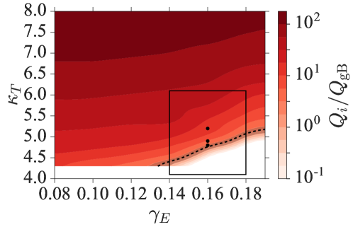
Figure 5: Ion heat flux $Q_{i}/Q_{\mathrm{gB}}$ as a function of $\kappa_{T}$ and $\gamma_{E}$ for all simulations with $\gamma_{E}>0$. The rectangular region indicates the range in $\kappa_{T}$ and $\gamma_{E}$ consistent with the experiment and measurement uncertainties. The dashed line indicates the value of $Q_{i}^{\exp}/Q_{\mathrm{gB}}$ and the shaded area the experimental uncertainty. The experiment is clearly near the turbulence threshold defined by $(\kappa_{T},\gamma_{E})$. The points indicate the parameter values for which the density-fluctuation fields are shown in figure 13.

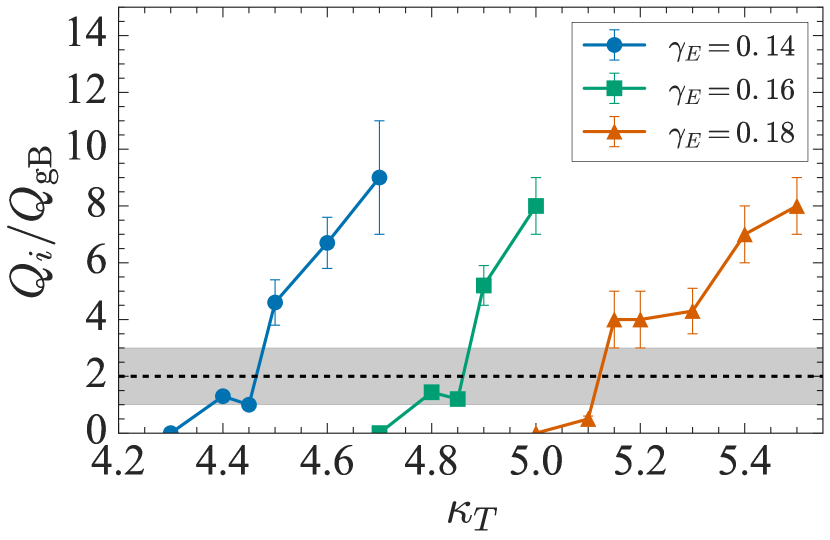
(a)

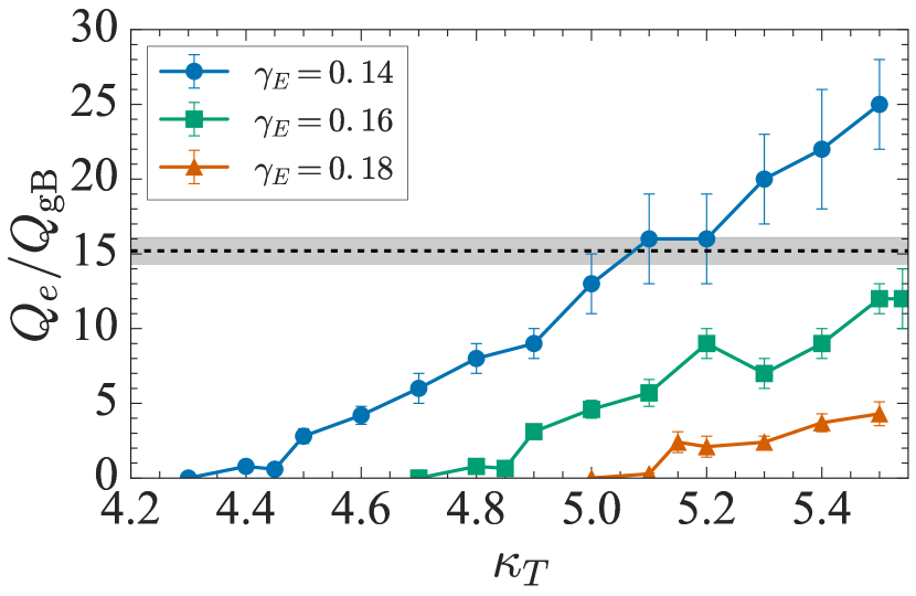
(b)

Figure 6: 6(a) Ion heat flux $Q_{i}/Q_{\mathrm{gB}}$ and 6(b) electron heat flux $Q_{e}/Q_{\mathrm{gB}}$ as a functions of $\kappa_{T}$ strictly within experimental uncertainty of $\kappa_{T}$ and $\gamma_{E}$, and close to the turbulence threshold. The shaded region in each plot indicates the experimental heat fluxes $Q_{i}^{\exp}/Q_{\mathrm{gB}}=2\pm 1$ and $Q_{e}^{\exp}/Q_{\mathrm{gB}}=15.2\pm 0.9$, determined from figure 3.

Figure 6(a) shows $Q_{i}/Q_{\mathrm{gB}}$ as a function of $\kappa_{T}$ strictly within the region of measurement uncertainty of $\kappa_{T}$ and $\gamma_{E}$, close to the turbulence threshold. The dashed line and shaded region indicate $Q_{i}^{\exp}/Q_{\mathrm{gB}}$ and its associated uncertainty. We see that there is a range of $\kappa_{T}$ and $\gamma_{E}$ values where we might expect $Q_{i}/Q_{\mathrm{gB}}$ to match $Q_{i}^{\exp}/Q_{\mathrm{gB}}$. From this figure, we can also identify several simulations that represent the marginally unstable cases in our parameter scan: $(\kappa_{T},\gamma_{E})=(4.4,0.14),(4.8,0.16),(5.1,0.18)$. We will consider these parameter values section 3.2, when studying the conditions necessary to reach a saturated turbulent state. Furthermore, we have a number of individual simulations that match the value of $Q_{i}^{\exp}/Q_{\mathrm{gB}}$. A list of these is given in table 2. We will investigate these simulations further when we make more detailed comparisons with the experiment, in section 4.

Figure 6(b) shows that the electron heat flux, $Q_{e}^{\exp}/Q_{\mathrm{gB}}$, is not fully captured by our nonlinear ion-scale simulations: namely, in our simulations, we observe $Q_{e}/Q_{i}\sim 0.6$, whereas from the experiment we expect $Q_{e}^{\exp}/Q_{i}^{\exp}\sim 7.6$ (see figure 3). It is likely that electron-scale turbulence [14, 28, 21, 22, 23, 68] is present in the real machine, while it cannot be resolved in our simulations, and that it dominates electron heat transport. Thus, given the likely existence of turbulence on both electron and ion scales, a programme of gyrokinetic simulations capturing electron and ion scales simultaneously would ideally be necessary. While individual such multiscale simulations have been performed [69, 70], we cannot afford the number of such simulations that would be necessary to carry out a parameter scan as extensive as we present in this paper. Instead, we will focus on local simulations of ion-scale turbulence, and compare the results from these simulations with ion-scale BES measurements from MAST.

Figure 7(a) shows the values of $Q_{i}/Q_{\mathrm{gB}}$ from figure 5 for several values of $\gamma_{E}$ as a function of $\kappa_{T}$, whereas figure 7(b) shows $Q_{i}/Q_{\mathrm{gB}}$ as a function of $\gamma_{E}$ for several values of $\kappa_{T}$. We see that an $O(1)$ change in $\kappa_{T}$ gives rise to an $O(10)$ change in $Q_{i}/Q_{\mathrm{gB}}$, and even more dramatically for changes in $\gamma_{E}$, which requires only an $O(0.1)$ change to cause $O(10)$ changes in the ion heat flux. An important conclusion from this figure is that the presence of flow shear does not significantly affect the stiffness of the transport, i.e., the rate of increase of $Q_{i}/Q_{\mathrm{gB}}$ with respect to $\kappa_{T}$, but only changes the threshold value of $\kappa_{T}$ above which turbulence is present. This increase in critical $\kappa_{T}$ without a change in the stiffness of $Q_{i}/Q_{\mathrm{gB}}$ with respect to $\kappa_{T}$ has been observed in numerical simulations of simplified ITG-unstable plasmas in the presence of flow shear [71, 32]. It is also in agreement with experimental [8, 9] and numerical [10] findings in the outer core of the JET experiment, which also showed that ion heat transport’s stiffness is not affected by an increase in $\gamma_{E}$, whereas the critical $\kappa_{T}$ threshold does increase with $\gamma_{E}$.

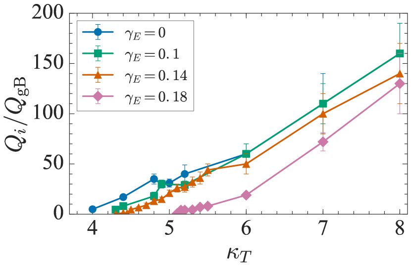
(a)

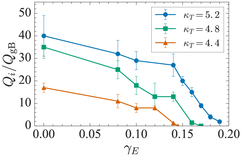
(b)

Figure 7: 7(a) Ion heat flux $Q_{i}/Q_{\mathrm{gB}}$ as a function of $\kappa_{T}$ for several values of $\gamma_{E}$. 7(b) $Q_{i}/Q_{\mathrm{gB}}$ as a function of $\gamma_{E}$ for several values of $\kappa_{T}$.

Table 2: Parameter values for simulations that match the experimental heat flux, $Q_{i}^{\exp}/Q_{\mathrm{gB}}=2\pm 1$.

$\kappa_{T}$	$\gamma_{E}$	$Q_{i}/Q_{\mathrm{gB}}$
4.4	0.14	$1.3\pm 0.1$
4.45	0.14	$1.0\pm 0.1$
4.8	0.16	$1.44\pm 0.05$
4.85	0.16	$1.2\pm 0.1$
5.15	0.18	$4\pm 1$
5.2	0.18	$4\pm 1$

3.2 Subcritical turbulence

We have found that in all our simulations with $\gamma_{E}>0$, small amplitude initial perturbations decayed (i.e. the system was linearly stable) and a finite initial perturbation was always required in order to ignite turbulence and reach a saturated turbulent state. Turbulence in MAST in the equilibrium configuration that we study here belongs to the class of subcritical systems [72, 35, 73, 36], where linear modes are formally stable, but may be transiently amplified by a given factor over a given time. If the transient amplification is sufficient for nonlinear interactions to become significant before the modes decay, then a turbulent state may emerge. This turbulent state persists provided the fluctuation amplitudes do not fall below some critical value (for example, by way of the chaotic evolution, with occasional large deviations from an average fluctuation level that characterises the turbulent state) below which they cannot be transiently amplified once again back to nonlinearly sustained saturated level.

In this work, we have assumed that other activity in the experiment (e.g. large-scale MHD modes or more virulent turbulence on neighbouring flux surfaces) can generate arbitrarily large perturbations as an initial condition to our system. For this reason, we have used the largest initial perturbation allowed by the numerical algorithm used in GS2, i.e., as large as possible without forcing the system to evolve the distribution function with time steps so small that the simulations would require prohibitively long simulation times. All nonlinear simulations presented in section 3.1 were run with such large initial conditions. For the regions where we have reported $Q_{i}=0$, we could not ignite turbulence using even the largest initial condition tolerated by the GS2 algorithm. In this section we will demonstrate the subcritical nature of the turbulence by investigating the effect of changing the amplitude of the initial perturbation in both linear and nonlinear simulations.

3.2.1 Minimum initial perturbation amplitude

We start by considering the nonlinear time evolution of a simulation at the nominal equilibrium parameters $(\kappa_{T},\gamma_{E})=(5.1,0.16)$. Figure 8(a) shows $Q_{i}/Q_{\mathrm{gB}}$ as a function of time for nonlinear simulations with increasing initial amplitude. These parameter values represent a simulation somewhat away from the turbulence threshold [see figure 5] and yet, for a range of initial amplitudes, we see that the system decays rapidly. This is a clear indication that the turbulence is subcritical. We see that there is a certain minimum initial perturbation amplitude starting from which it is possible for the system to reach a saturated state, rather than decay. Importantly, for simulations that do reach a saturated state, the level of saturation does not depend on the amplitude of the initial perturbation.

3.2.2 Finite life time of turbulence

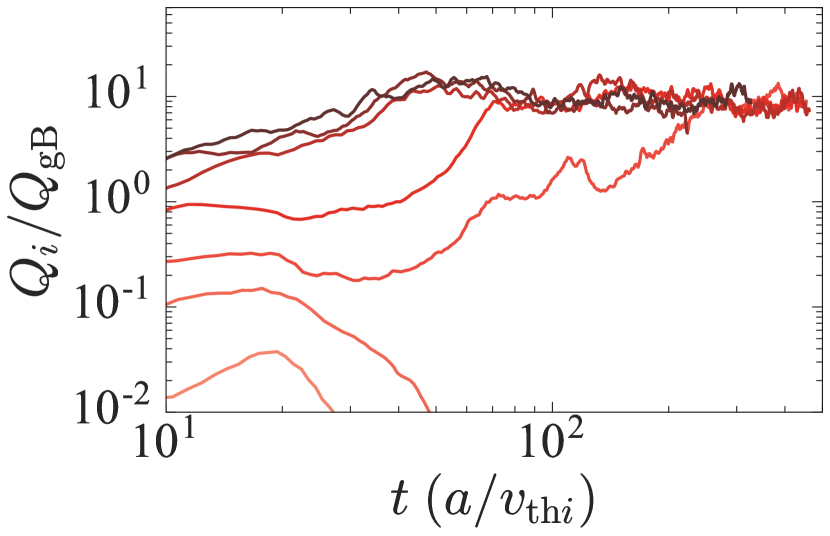
(a)

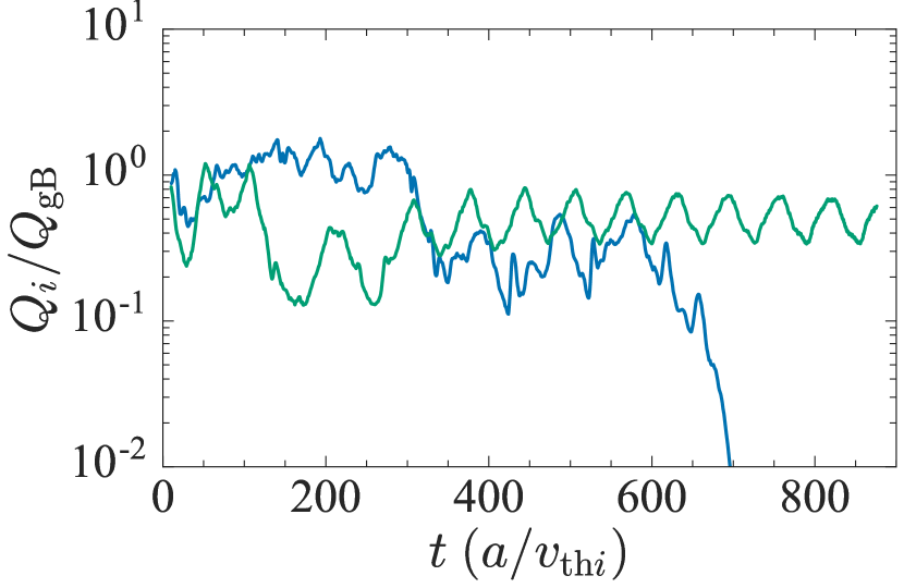
(b)

Figure 8: 8(a) Ion heat flux $Q_{i}/Q_{\mathrm{gB}}$ as a function of time for different initial-perturbation amplitudes for $(\kappa_{T},\gamma_{E})=(5.1,0.16)$, keeping all other parameters the same. 8(b) $Q_{i}/Q_{\mathrm{gB}}$ as a function of time for two identical simulations at $(\kappa_{T},\gamma_{E})=(5.1,0.18)$. The difference between the time series shown as the blue and green lines is the realisation of the random noise with which GS2 initialised these simulation. Beyond $t=300$ $(a/v_{\mathrm{th}i})$, the simulations seem to converge to a similar average value before one is abruptly quenched due to the amplitudes falling below the critical values required to sustain a saturated state.

A large initial perturbation is not sufficient to guarantee that a subcritical system continues in a statistically steady state indefinitely. In simulations with equilibrium parameters close to the turbulence threshold, we found that turbulence could be quenched at a seemingly unpredictable time. For example, figure 8(b) shows the time trace of $Q_{i}/Q_{\mathrm{gB}}$ for two identical simulations at the parameter values $(\kappa_{T},\gamma_{E})=(5.1,0.18)$, close to the turbulence threshold. These simulations were initialised with random noise of a given amplitude in each Fourier mode and the only difference between the two simulations is the realisation of this random noise. We see the simulations saturate at a similar level beyond $t=300$ $(a/v_{\mathrm{th}i})$, but then one of them abruptly decays. This is another indication that the system is subcritical: the decaying simulation has fallen below the critical amplitude needed to sustain turbulence. Practically, in this study, we decided that a simulation reached a saturated state if the heat flux evolved at a roughly constant value for at least $200$ $(a/v_{\mathrm{th}i})$.

The finite life time of turbulence in subcritical systems is well established in some hydrodynamic systems, such as fluid flow in a pipe [74]. By running a large number of identical pipe-flow experiments [75, 76, 77] and numerical simulations [74, 76, 78, 77], it was shown that the “life time” of subcritical turbulence (the characteristic time that elapses before turbulence decays to laminar flow) is a function of the Reynolds number. The Reynolds number in pipe flows quantifies the “distance from the turbulence threshold”. In particular, it was shown that the larger its value (i.e., the further the system is from the turbulence threshold), the longer the turbulence is likely to persist. More recently, the same phenomenon of finite turbulence lifetime was observed in MHD simulations of astrophysical Keplerian shear flow systems [79], where the distance from threshold was characterised by the magnetic Reynolds number and the turbulence persists longer for large values of this parameter.

Given the above considerations, we would also expect the subcritical turbulence considered here to persist for longer times at larger values of $Q_{i}/Q_{\mathrm{gB}}$. The pipe-flow and astrophysical studies referred to above relied on running many experiments and simulations in order to build up sufficient statistics to determine the dependence of the turbulence lifetimes on the system parameters. With the high resolutions demanded by nonlinear gyrokinetic simulations of plasmas in the core of tokamaks we are neither able to run a sufficient number of simulations nor to run them for a sufficient amount of time to determine the turbulence lifetimes for our system. However, this may be possible in future, given advances in computing and numerics or through the use of reduced models.

3.2.3 Transient growth of perturbations

A system can reach a saturated turbulent state despite being stable to infinitesimal perturbations due to transient growth of (large enough) finite perturbations. This transient growth can sustain turbulence provided perturbations reach an amplitude sufficient for nonlinear interaction. Having established the subcritical nature of the system, the question we would now like to address is how much transient growth is sufficient for the system to reach a turbulent state. We have already seen which values of $\kappa_{T}$ and $\gamma_{E}$ lead to a turbulent state [see figure 5] and we now investigate transient growth of perturbations via linear GS2 simulations at these values of $\kappa_{T}$ and $\gamma_{E}$.

We performed an extensive series of linear simulations and calculated the time evolution of the electrostatic potential $\varphi$ as a function of $k_{y}\rho_{i}$, $\kappa_{T}$, and $\gamma_{E}$. Figure 9(a) shows an example of the time evolution of $\varphi$ (at $k_{y}\rho_{i}=0.2$ and $\gamma_{E}=0.16$) for a range of $\kappa_{T}$, normalised to the value of $\varphi$ at the time (called $t=0$) when the flow shear is switched on, that is, $\varphi_{N}^{2}(t)=\varphi^{2}(t)/\varphi^{2}(0)$. We have averaged $\varphi$ over $k_{x}$. Figure 9(a) illustrates the phenomenon of transient growth in a subcritical system and we see that, as $\kappa_{T}$ is increased, the system exhibits stronger transient growth. At $\gamma_{E}=0.16$, we saw in figure 5 that turbulence could be sustained at $\kappa_{T}\gtrsim 4.8$. Indeed, figure 9(a) shows that there is only a marginal amount of transient growth at $\kappa_{T}\approx 4.8$.

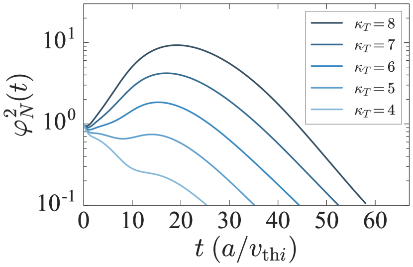
(a)

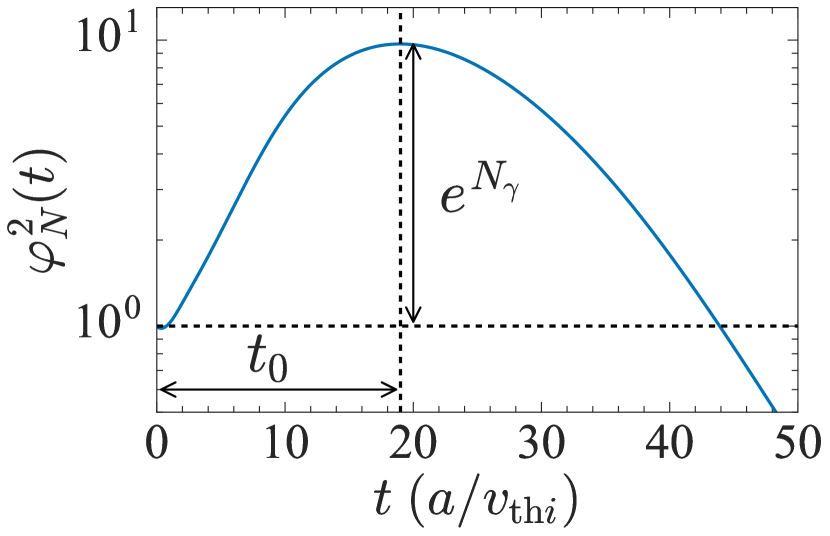
(b)

Figure 9: 9(a) Transient growth of initial perturbations of the electrostatic potential $\varphi^{2}_{N}(t)$ (normalised to the time at which flow shear is switched on) at $\gamma_{E}=0.16$, for a range of $\kappa_{T}$ values. These time evolutions were obtained from purely linear simulations for $k_{y}\rho_{i}=0.2$, approximately the wavenumber that gives the largest transient growth [see figure 10(a)], and summed over $k_{x}$. As $\kappa_{T}$ is increased, the strength of the transient growth also increases. 9(b) $\varphi^{2}_{N}(t)$ as a function of time for a strongly growing mode at $(\kappa_{T},\gamma_{E},k_{y}\rho_{i})=(8,0.16,0.2)$ further illustrating transient amplification. The total amplification factor is $e^{N_{\gamma}}$ and the time taken to reach maximal amplification is $t_{0}$.

3.2.4 Characterising transient growth

For linear simulations exhibiting transient growth, one cannot define a “linear growth rate”, as one does for linear simulations with $\gamma_{E}=0$ where $\varphi(t)$ grows exponentially. However, methods for determining an “effective” linear growth rate have been outlined in Ref. [28] and [35]. Here, we follow Ref. [35] and use the “transient-amplification factor” as a measure of the vigour of the transient growth. For a total amplification factor $e^{N_{\gamma}}$, the amplification exponent $N_{\gamma}$ is defined by

$$N_{\gamma}=\frac{1}{2}\ln\frac{\varphi^{2}(t_{0})}{\varphi^{2}(0)}=\int_{0}^{t_{0}}\differential t\gamma(t),$$ (12)

where $t_{0}$ is the time taken to reach the maximum amplification, and $\gamma(t)$ is the time-dependent growth rate. These quantities are illustrated in Figure 9(b), which shows a typical linear simulation with strong amplification, with $e^{N_{\gamma}}$ and $t_{0}$ indicated.

It was argued in Ref. [35] that the parameters $N_{\gamma}$ and $t_{0}$ determine whether turbulence can be sustained, in the following way. Perturbations grow only transiently because flow shear leads to $k_{x}(t)=k_{x}(0)-\gamma_{E}k_{y}t$ being swept from the region where perturbations are unstable to larger values, where they are stabilised by dissipation. If nonlinear interactions scatter energy back into the unstable modes before perturbations decay they can be transiently amplified once again, and so on. In this way, a nonlinear saturated state can be sustained. The typical timescale for nonlinear interactions is the nonlinear decorrelation time $\tau_{\mathrm{NL}}\sim 1/k_{\perp}V_{E}$, where $k_{\perp}$ is the typical perpendicular wave number, and $V_{E}$ is given by (7). To sustain turbulence, transient growth should last at least as long as one nonlinear decorrelation time:

$$\begin{split}t_{0}&\gtrsim\tau_{\mathrm{NL}}.\end{split}$$ (13)

At the same time, the rate of amplification should be at least comparable to the nonlinear decorrelation rate:

$$\frac{N_{\gamma}}{t_{0}}\gtrsim\frac{1}{\tau_{\mathrm{NL}}}.$$ (14)

Combining (13) and (14), we see that a sustained turbulent state requires

$$N_{\gamma}\gtrsim 1.$$ (15)

3.2.5 Conditions for the onset of subcritical turbulence

We now want to estimate the critical values of $N_{\gamma}$ and $t_{0}$ above which turbulence is triggered and a saturated state can be established in our system. Figure 10 shows $N_{\gamma}$ and $t_{0}$ as functions of $k_{y}\rho_{i}$ for a range of different $\kappa_{T}$ values at $\gamma_{E}=0.16$ (only wave numbers up to $k_{y}\rho_{i}=1.3$ are shown, because numerical dissipation effectively suppresses transient growth beyond this value). As a point of reference, for $\gamma_{E}=0.16$, the transition to turbulence occurs at $\kappa_{T}\approx 4.8$ [see figure 6(a)]. For the linear simulations in figure 10, we see a relatively smooth increase in $N_{\gamma}$ and $t_{0}$ as $\kappa_{T}$ is increased across this nonlinear threshold, with larger transient amplification and modes with smaller $k_{y}\rho_{i}$ experiencing amplification over a longer time period.

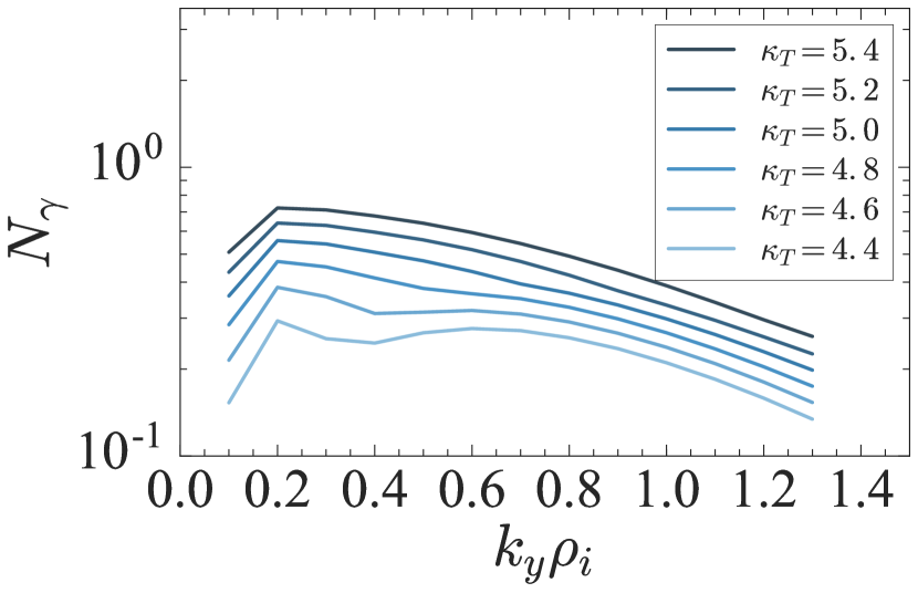
(a)

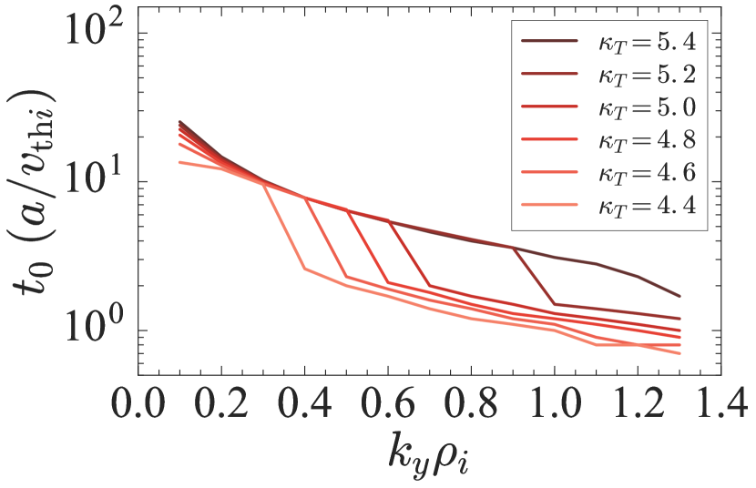
(b)

Figure 10: 10(a) The transient-amplification factor $N_{\gamma}$, defined in (12), for a range of values of $\kappa_{T}$ at $\gamma_{E}=0.16$. $N_{\gamma}$ increases smoothly with increasing $\kappa_{T}$ as the nonlinear threshold is passed. 10(b) Time $t_{0}$ taken to reach maximum amplification for a range of values of $\kappa_{T}$, also at $\gamma_{E}=0.16$. Increasing $\kappa_{T}$ leads to transient amplification lasting for a longer time.

To investigate the conditions for the onset of turbulence, we consider $N_{\gamma}$ and $t_{0}$ for the marginally unstable simulations identified in section 3.1. Figures 11(a) and 11(b) show $N_{\gamma}$ and $t_{0}$ as functions of $k_{y}\rho_{i}$ for $(\kappa_{T},\gamma_{E})=(4.4,0.14),(4.8,0.16),(5.1,0.18)$. We see that both $N_{\gamma}$ and $t_{0}$ are roughly the same for our marginally unstable simulations, suggesting that the values shown in Figures 11(a) and 11(b) are indeed the critical values necessary for the onset of turbulence.

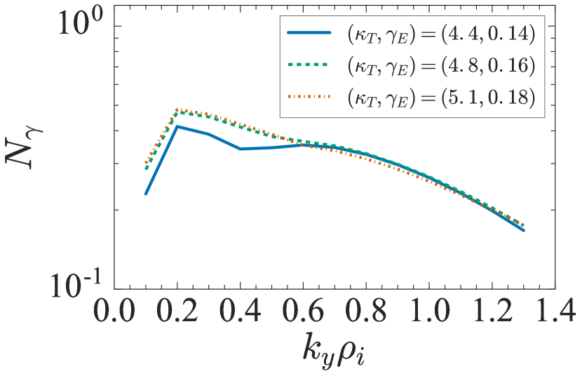
(a)

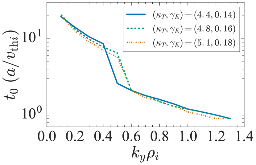
(b)

Figure 11: 11(a) Transient-amplification factor $N_{\gamma}$ [see equation (12)] and 11(b) transient-amplification time $t_{0}$ for the three marginal simulations identified in section 3.1. The values of $N_{\gamma}$ and $t_{0}$ that correspond to the marginally unstable equilibria are approximately the same, suggesting that these represent the critical values required for the system to reach a saturated turbulent state.

We see from figures 10(a) and 11(a) that the maximum $N_{\gamma}$ is at $k_{y}\rho_{i}\approx 0.2$ and we consider its value here to to determine the critical condition. Figure 12 shows the maximum value $N_{\gamma,\max}$ of the transient-amplification factor as a function of $\kappa_{T}$. The marked simulations are for the critical values of $\kappa_{T}$ above which turbulence can be sustained, given a sufficiently large initial perturbation amplitude. Figure 12 shows that $N_{\gamma,\max}$ scales linearly with $\kappa_{T}$ for each $\gamma_{E}$, with higher values of $\gamma_{E}$ resulting in lower values of $N_{\gamma,\max}$. The other important feature is that the values of $N_{\gamma,\max}$ at the critical values of $\kappa_{T}$ are similar, giving an approximate critical condition: $N_{\gamma,\max}\sim 0.4$. This value of $N_{\gamma,\max}$ is comparable to that found in previous work [35, 73].

Returning to figure 11(b), and assuming that low-$k_{y}$ modes are the important ones for sustaining turbulence, it is reasonable to estimate that the onset of turbulence requires $t_{0}\gtrsim 10$ $(a/v_{\mathrm{th}i})$. We will return to the comparison of $t_{0}$ with $\tau_{\mathrm{NL}}$ after estimating $\tau_{\mathrm{NL}}$ in section 4.4.4, where we confirm that $t_{0}\gtrsim\tau_{\mathrm{NL}}$ and, therefore, that a sustained turbulent state requires an amplification time comparable to (or greater than) the nonlinear decorrelation time.

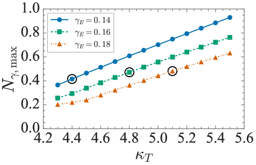
Figure 12: Maximum transient-amplification factor $N_{\gamma,\max}$ versus $\kappa_{T}$ for three values of $\gamma_{E}$ within the range of experimental uncertainty. The simulations circled in black represent the critical values of $\kappa_{T}$ above which turbulence can be sustained, suggesting the onset of turbulence occurs at $N_{\gamma,\max}\simeq 0.4$.

We have shown that the changes in $N_{\gamma}$ and $t_{0}$ are relatively smooth as the turbulence threshold is surpassed (determined from our simulations in section 3.1), suggesting nonlinear simulations are essential in predicting the exact transition to turbulence. In the next section, we will investigate the nature of this transition by considering the real-space structure of the turbulence in our nonlinear simulations.

3.3 Structure of turbulence close to and far from the threshold

Having established the subcritical nature of the system, we now investigate the consequences for the structure of turbulence. We will argue that our subcritical system supports the formation of long-lived coherent structures close to the turbulence threshold. In this context, we take “coherent” to mean turbulent structures that remain distinct in space as they move through the simulation domain and exist for (most of) the duration of the simulation (see section 3.3.1). We will also show that the heat flux is proportional to the product of number of these structures and their maximum amplitude, and that the properties of the turbulence are characterised by the “distance from threshold” (as opposed to the specific values of the stability parameters $\kappa_{T}$ and $\gamma_{E}$), as measured, for example, by the turbulent ion heat flux. We previously reported some of these results in Ref. [37], based on the simulations in this study, and provide a more comprehensive description here.

3.3.1 Coherent structures in the near-marginal state

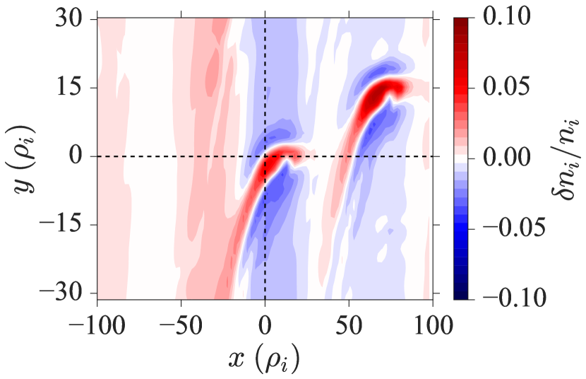
(a)

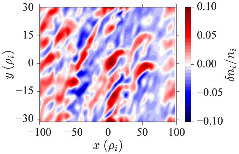
(b)

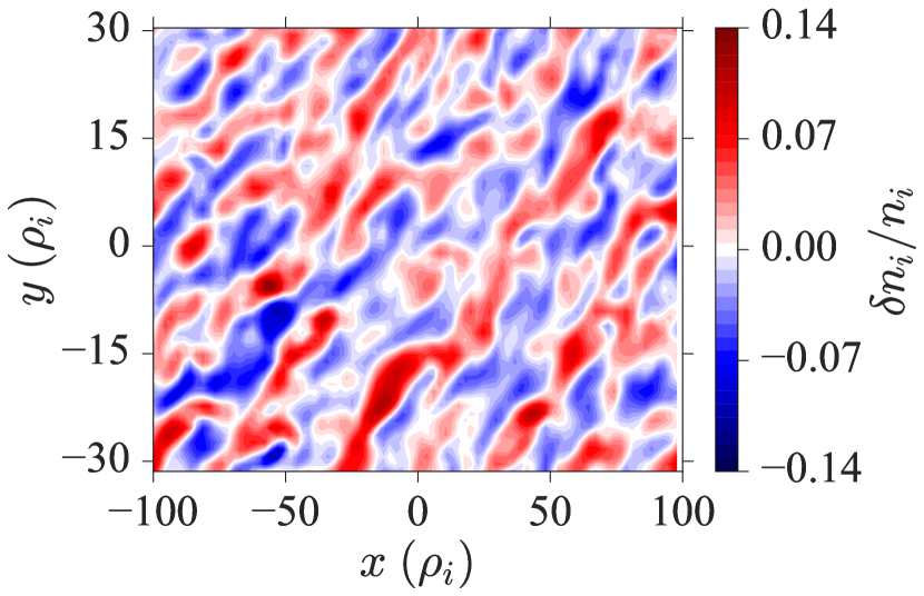
(c)

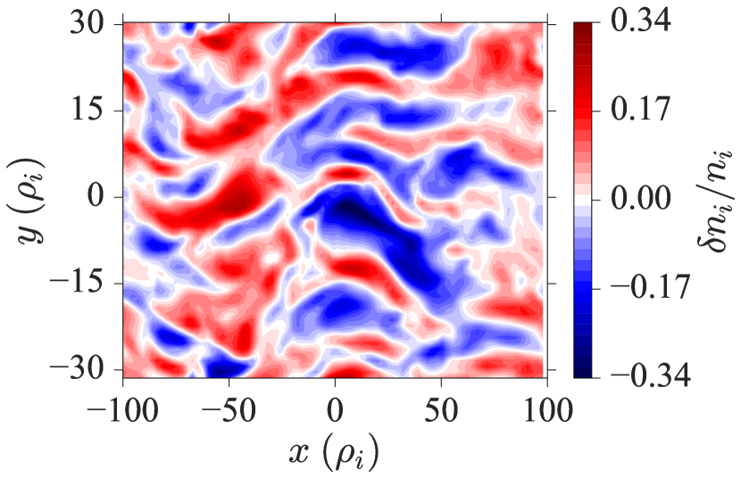
(d)

Figure 13: Density-fluctuation field $\delta n_{i}/n_{i}$ at the outboard midplane of MAST as a function of the local GS2 coordinates $x$ and $y$, for four combinations of stability parameters. 13(a) Near-threshold turbulence, $(\kappa_{T},\gamma_{E})=(4.8,0.16)$. The dashed lines indicate the planes of constant $x$ and $y$ used to demonstrate the parallel structure in figure 16. 13(b) Turbulence intermediate between the near-threshold and strongly driven cases, $(\kappa_{T},\gamma_{E})=(4.9,0.16)$. 13(c) Strongly driven turbulence, $(\kappa_{T},\gamma_{E})=(5.2,0.16)$. 13(d) Turbulence without flow shear, $(\kappa_{T},\gamma_{E})=(5.2,0)$, showing strong zonal flows.

Figure 13 shows the density-fluctuation field $\delta n_{i}/n_{i}$ at the outboard midplane of MAST as a function of the local GS2 coordinates $x$ and $y$. The simulations shown in figures 13(a)–13(c) are marked by points in figure 5 and, importantly, all three are well within the region of experimental uncertainty. We have chosen four combinations of the stability parameters $(\kappa_{T},\gamma_{E})$ as the system is taken away from the turbulence threshold: $(4.8,0.16)$, which is close to the turbulence threshold [figure 13(a)], $(4.9,0.16)$, an intermediate case between the marginal and strongly driven turbulence [figure 13(b)], $(5.2,0.16)$, a strongly driven case further from the threshold [figure 13(c)], and $(5.2,0)$, a case without flow shear [figure 13(d)], representative of the normal, supercritical ITG turbulence that has been thoroughly studied in the past [80, 81, 82]. For the same four cases, figures 14 and 15 show the perturbed radial ${\bf\it E}\times{\bf\it B}$ velocity $V_{Er}$ and the perpendicular temperature-fluctuation $\delta T_{\perp i}/T_{\perp i}\equiv a/\rho_{i}\delta T_{\perp i}/T_{\perp i}$ fields. We have calculated $V_{Er}$ velocity by taking the radial component of (7), given by (see equation (3.42) in Ref [66])

$$V_{Er}=\frac{c}{aB_{\mathrm{ref}}}\frac{1}{|\nabla\psi|}\quantity|\partialderivative{\psi}{r}|_{r_{0}}\partialderivative{\varphi}{y},$$ (16)

recalling that $a$ is the half diameter of the LCFS, $B_{\mathrm{ref}}$ is the toroidal magnetic field at the magnetic axis, $\psi$ is the poloidal magnetic flux, and $r=D/2a$.

As the system is taken away from the threshold, the nature of the fluctuation field changes as follows. The near-threshold state [figure 13(a)] is dominated by coherent, long-lived (see figure 17) structures that are at high intensity compared to the background fluctuations. As $\kappa_{T}$ is slightly increased (in this case by only 0.1), these structures become more numerous [figure 13(b)], but have roughly the same maximum amplitude: ${(\delta n_{i}/n_{i})}_{\max}\sim 0.08$. In contrast, the strongly driven state [far from threshold; figure 13(c)] exhibits a more conventional turbulence, characterised by many interacting eddies with larger amplitudes.

These simulations are typical of the cases close to and far from the turbulence threshold, i.e., in simulations near the threshold, we always find sparse but well-defined coherent structures that survive against a backdrop of weaker fluctuations [with the important exception of the case of $\gamma_{E}=0$ shown in figure 13(d)]. Likewise, for all cases where the system is taken away from the threshold by increasing $\kappa_{T}$, or decreasing $\gamma_{E}$, the transition from coherent structures to strongly driven interacting eddies occurs the same way: the structures become more numerous, while maintaining roughly the same amplitude, until they fill the entire domain, interact with each other, and break up. For parameter values far from the threshold, we observe no discernible coherent structures, but rather strongly time-dependent fluctuations with amplitudes that increase with $\kappa_{T}$.

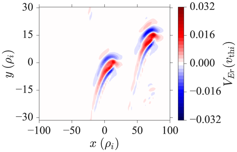
(a)

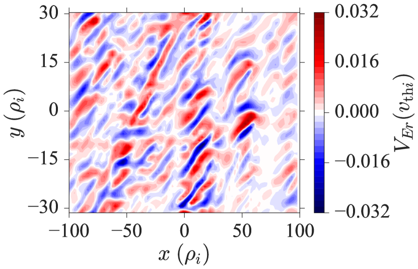
(b)

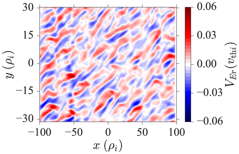
(c)

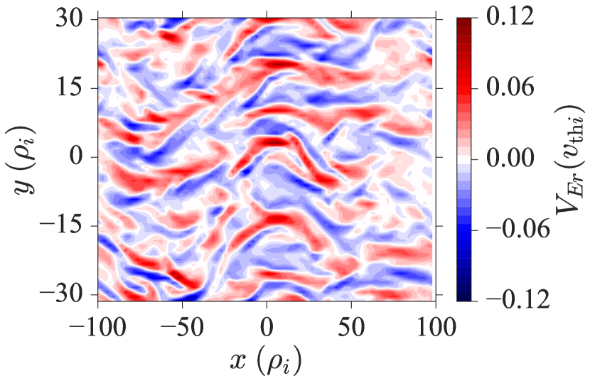
(d)

Figure 14: Radial ${\bf\it E}\times{\bf\it B}$ velocity $V_{Er}$ at the outboard midplane of MAST as a function of the local GS2 coordinates $x$ and $y$ for the same equilibrium parameters as in figure 13.

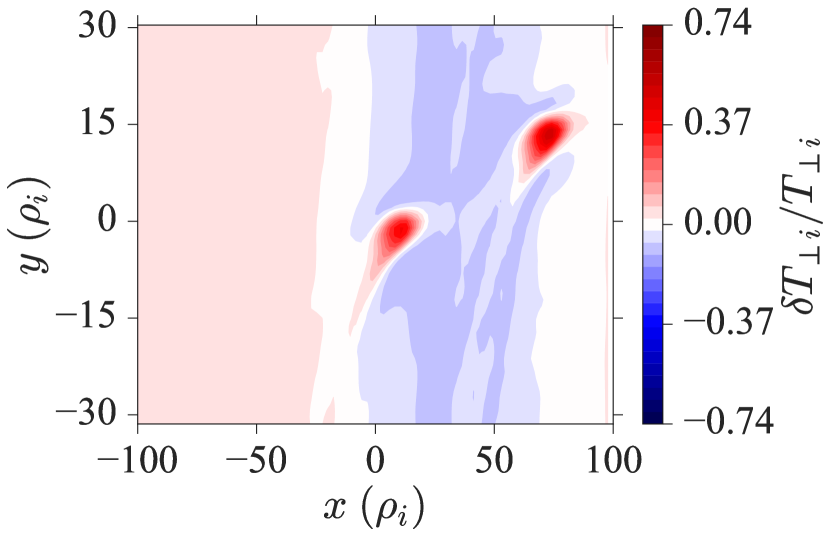
(a)

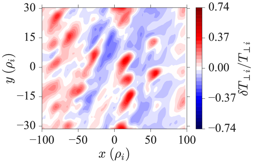
(b)

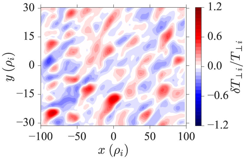
(c)

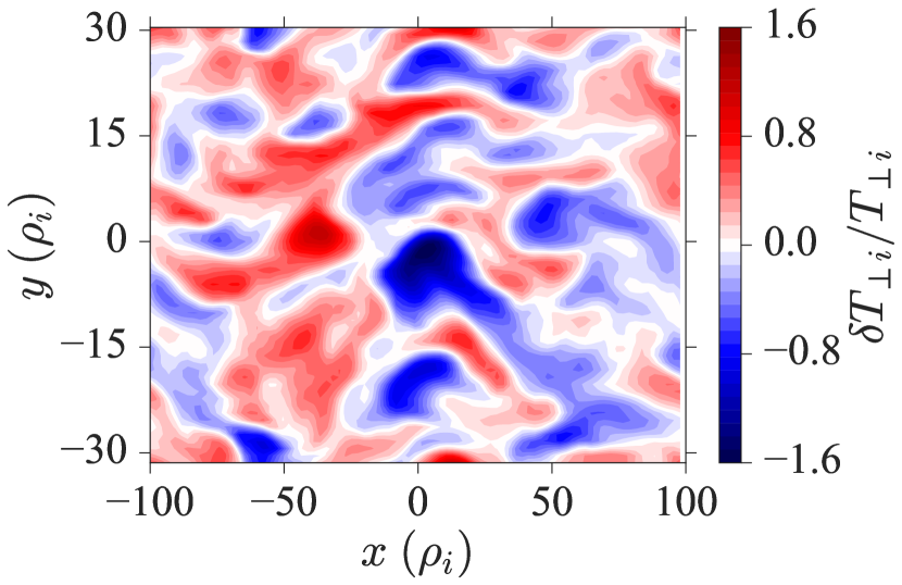
(d)

Figure 15: Perpendicular-temperature fluctuation field $\delta T_{\perp i}/T_{\perp i}$ at the outboard midplane of MAST as a function of the local GS2 coordinates $x$ and $y$ for the same equilibrium parameters as in figure 13.

We complete our description of these coherent structures by examining their parallel extent and their motion. Figure 16 shows two views of the coherent structures from figure 13(a) in the parallel direction (which in GS2 is quantified by the poloidal angle $\theta$): at constant $y$ [figure 16(a)] and at constant $x$ [figure 16(b)]. It is clear that the coherent structures are elongated in the parallel direction and have an amplitude much larger than the background fluctuations.

The motion of the coherent structures results from a combination of the background plasma flow, and a radial drift of the structures themselves. Importantly, they are long-lived as we will now show by looking at their motion in time. Figures 17(a) and 17(b) show $\delta n_{i}/n_{i}$ for a marginal nonlinear simulation at $(\kappa_{T},\gamma_{E})=(5.1,0.18)$, which has only one coherent structure, as a function of $(t,x)$ and $(t,y)$ (taking the maximum value of $\delta n_{i}/n_{i}$ in the other direction), respectively. Figure 17(a) shows the radial motion of the structure across the domain, which the structure crosses in a time of roughly $50~{}(a/v_{\mathrm{th}i})$, and illustrates the long-lived nature of coherent structures close to the turbulence threshold (recalling that the GS2 domain is periodic in $x$ and $y$). We see that the structure exists for $t>100~{}(a/v_{\mathrm{th}i})$. The radial motion of the structure in figure 17(a) has a constant velocity: fitting its trajectory with a straight line (the dashed line) gives $v_{x}=3.150\pm 0.009$ $\rho_{*}v_{\mathrm{th}i}$ (where $\rho_{*}=\rho_{i}/a=1/100$, given that $\rho_{i}=6.08\times 10^{-3}$ m and $a=0.58$ m). Figure 17(b) shows the poloidal advection of the structure with a much shorter poloidal crossing time of roughly $5~{}(a/v_{\mathrm{th}i})$. The poloidal motion of the structure is due to the combination of poloidal advection by the mean flow (remembering that, since we have moved to the rotating frame, the flow is zero at $x=0$) and the radial drift of the structures. As we saw in figure 17(a), $v_{x}$ is constant and the radial position is given by $x(t)=v_{x}t$. The poloidal advection due to the flow shear is given by $v_{y}(t)=\gamma_{E}x(t)$ and so the direction of the flow shear reverses at $x=0$. Combining the expressions for $x(t)$ and $v_{y}(t)$ and integrating, we find that $y(t)\propto\gamma_{E}v_{x}t^{2}$, and, as shown by the dashed line in figure 17(b), this describes the poloidal motion of the structures, which indeed reverses direction at $x=0$.

The coherent structures in the marginal case, such as the one described above, are unlike the strongly interacting eddies in the cases far from the turbulence threshold and are more likely to constitute a nonlinear travelling wave (soliton-like) solution to the gyrokinetic equation. However, more work is needed to develop an analytic description of these structures.

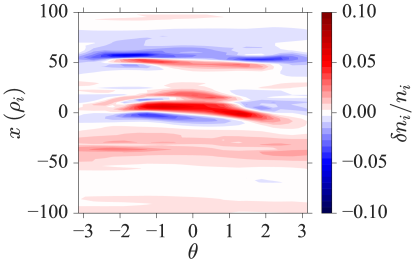
(a)

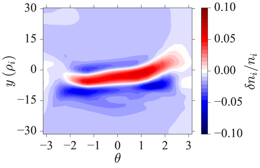
(b)

Figure 16: 16(a) Density-fluctuation field $\delta n_{i}/n_{i}$ in the $x$-$z$ plane at $y=0$. 16(b) Density-fluctuation field $\delta n_{i}/n_{i}$ in the $y$-$z$ plane at $x=0$. Both plots are for the same simulation and at the same time as in figure 13(a), where the corresponding planes are indicated by the dashed lines. The parallel direction in GS2 is quantified by the poloidal angle $\theta$.

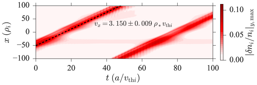
(a)

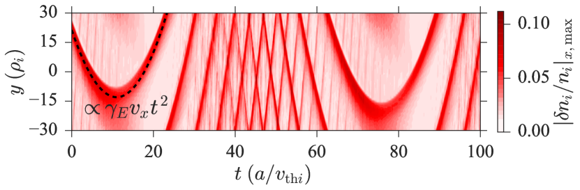
(b)

Figure 17: Density-fluctuation field $\delta n_{i}/n_{i}$ as a function of 17(a) $x$ and $t$ (taking the maximum in the $y$ direction) and 17(b) $y$ and $t$ (taking the maximum in the $x$ direction) for a marginally unstable case with $(\kappa_{T},\gamma_{E})=(5.1,0.18)$, which contains only one coherent structure. The structure is advected both radially and poloidally. The GS2 domain is periodic in $x$ and $y$ and so this is the same structure throughout the entire time period shown. The dashed line in 17(a) indicates $x=v_{x}t$, and in 17(b) it indicates $y\propto\gamma_{E}v_{x}t$, showing that the poloidal advection is due to the flow associated with the shear $\gamma_{E}$.

3.3.2 $Q_{i}/Q_{\mathrm{gB}}$ as an order parameter

The results in section 3.3.1 suggest that the nature of the turbulence is determined by how far the system is from the turbulence threshold. This means perhaps that the important metric that should be used to quantify the state of the system is the “distance from threshold” and not the specific values of $\kappa_{T}$ and $\gamma_{E}$ (although both can be used to control the distance from threshold). The ion heat flux $Q_{i}/Q_{\mathrm{gB}}$ is a strong function of $\kappa_{T}$ and $\gamma_{E}$, increasing monotonically as the system is taken away from the threshold [see figure 5], so we can use $Q_{i}/Q_{\mathrm{gB}}$ as a control parameter to measure the distance from the threshold. In sections 3.3.3 and 3.3.4, we will quantify the change in the nature of the turbulence, namely, the change in the amplitude and number of coherent structures, for our parameter scan and show that the distance from threshold is indeed the relevant order parameter.

3.3.3 Maximum amplitude

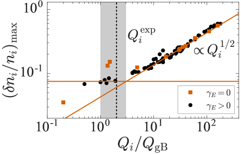
Figure 18: Maximum amplitude of the density fluctuations versus $Q_{i}/Q_{\mathrm{gB}}$. The naive scaling (17), $\delta n_{i}/n_{i}\propto Q_{i}^{1/2}$, is shown for reference and holds far from threshold, whereas for small values of $Q_{i}/Q_{\mathrm{gB}}$ (around and below the experimental value $Q_{i}^{\exp}$), the amplitude becomes independent of $Q_{i}/Q_{\mathrm{gB}}$.

Here, we investigate how the amplitude of the density fluctuations change with the distance from threshold. For near-threshold cases, such as the one shown in figure 13(a), the dominant features are the coherent structures, which have high densities compared to the background fluctuations. In order to capture the amplitude of these structures, we measure the maximum amplitude of the density field, as opposed to an $(x,y)$-averaged one, which would be small because of the relatively small volume taken up by the coherent structures. Figure 18 shows the maximum amplitude ${(\delta n_{i}/n_{i})}_{\max}$, maximised over the $(x,y)$-plane and averaged over time, versus $Q_{i}/Q_{\mathrm{gB}}$ for the entire set of simulations in our parameter scan.

The striking feature of figure 18 is that ${(\delta n_{i}/n_{i})}_{\max}$ hits a finite “floor” as $Q_{i}/Q_{\mathrm{gB}}$ approaches and goes below its experimental value. This coincides with the appearance of the long-lived structures such as those shown in figure 13(a). This floor is absent in simulations with $\gamma_{E}=0$, suggesting that the turbulence with $\gamma_{E}=0$ is fundamentally different close to the turbulence threshold (as indeed also suggested by the absence of coherent structures).

Far from the turbulence threshold, we can construct from (11) a naive estimate of the relationship between $Q_{i}/Q_{\mathrm{gB}}$ and $\delta n_{i}/n_{i}$:

$$\frac{Q_{i}}{Q_{\mathrm{gB}}}\sim\frac{a^{2}}{\rho_{i}^{2}}\frac{\delta T_{i}}{T_{i}}\frac{V_{Er}}{v_{{\mathrm{th}}i}}\sim k_{y}\rho_{i}{\left(\frac{\delta n_{i}}{n_{i}}\right)}^{2},$$ (17)

assuming that fluctuations of $\varphi$ are related (by order of magnitude) to the electron (and, therefore, ion) density via the Boltzmann response $e\varphi/T_{e}\sim\delta n_{e}/n_{e}$ and that ion temperature and density fluctuations are approximately proportional to each other (cf. figures 13 and 15). The scaling $\delta n_{i}/n_{i}\propto Q_{i}^{1/2}$ that follows from (17) assuming that $k_{y}\rho_{i}$ is not a strong function of $Q_{i}$ is indicated by the red line in figure 18, and describes well the scaling away from the threshold. We also see that $\gamma_{E}=0$ and $\gamma_{E}>0$ simulations are similar away from the threshold.

The above results can be understood as follows. In the case of supercritical turbulence, one typically observes smaller fluctuation amplitudes all the way to the turbulence threshold – there is no minimum amplitude required to sustain turbulence. In contrast, figure 18 shows that, for the subcritical turbulence that we are investigating, the maximum fluctuation amplitude stays constant as we approach the threshold. This is because there is a critical value required in order to sustain a saturated nonlinear state – indeed, if the amplitude dropped below a certain value in a subcritical system, all perturbations would decay. However, even as the fluctuation amplitude stays constant, the heat flux decreases as the threshold is approached. The system can satisfy the requirement of finite amplitude while simultaneously allowing the heat flux to decrease through a reduction of the volume taken up by finite amplitude turbulence. As we demonstrate in the next section, this is achieved via a reduction in the number of coherent structures.

3.3.4 Structure counting

(a)

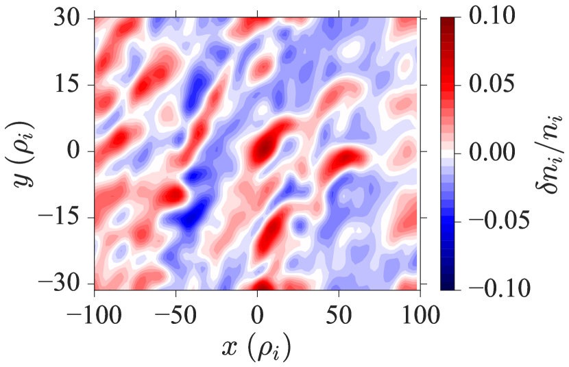
(b)

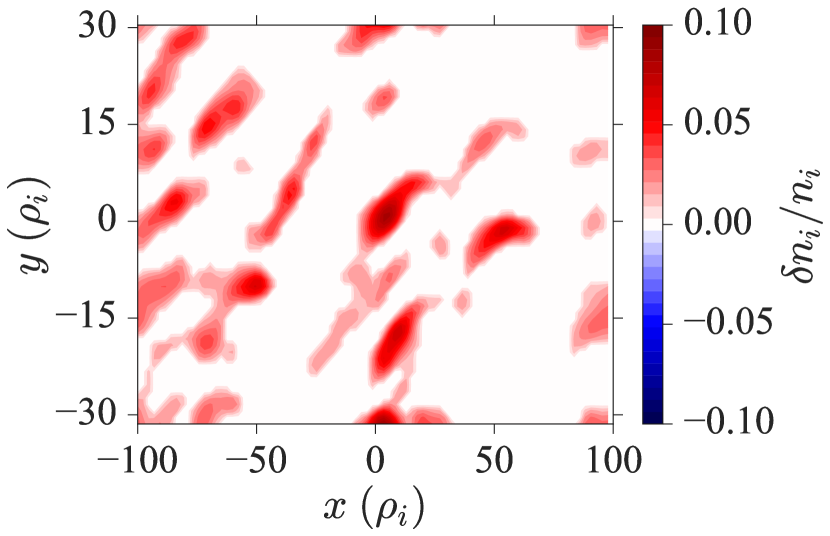
(c)

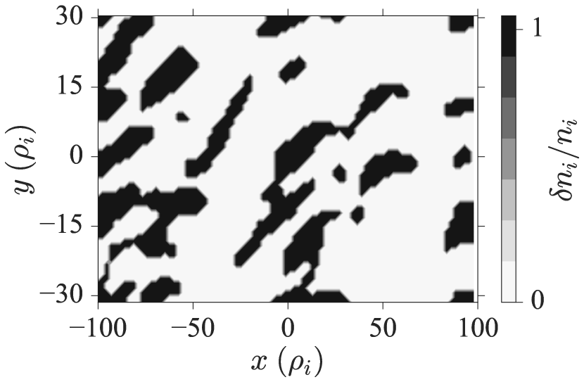
(d)

Figure 19: Stages of the structure-counting procedure: 19(a) the original density-fluctuation field [as in figure 13(b)]; 19(b) the same field after the application of a Gaussian filter to smooth the structures; 19(c) after the application of a 75% threshold function; 19(d) after setting $\delta n_{i}/n_{i}>0$ values to 1 for simplicity. The image-labelling algorithm is then applied to 19(d) and returns $19$ structures for this case.

We quantify the changes in volume taken up by the finite-amplitude structures by measuring the typical number of these structures in our simulations as a function of the distance from threshold. We follow the “structure-counting” methods first described in [37], which involve the following steps, illustrated in figure 19.

As a pre-processing step we apply a Gaussian image filter with a standard deviation of the order of the grid scale. We then set all density-field values below a certain percentile (here 75% of the maximum amplitude) to 0 and above it to 1. The level of this threshold function is somewhat arbitrary and the exact number of structures will depend on this level, but not the trend as a function of our equilibrium parameters. After applying the threshold function, we are left with an array of 1s representing our structures against a background of 0s. We then remove structures below 10% of the mean structure size as a post-processing step to avoid the counting of spurious small isolated blobs of high density. To count the structures, we employ a general-purpose image processing package scikit-image [83], which implements an efficient labelling algorithm [84], then used by us to label connected regions. In figure 19, the image-labelling algorithm found $19$ structures.

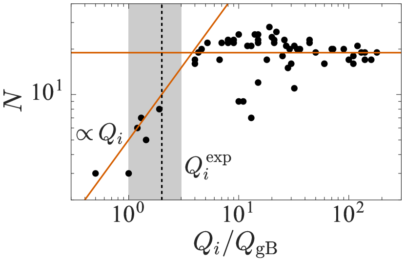
(a)

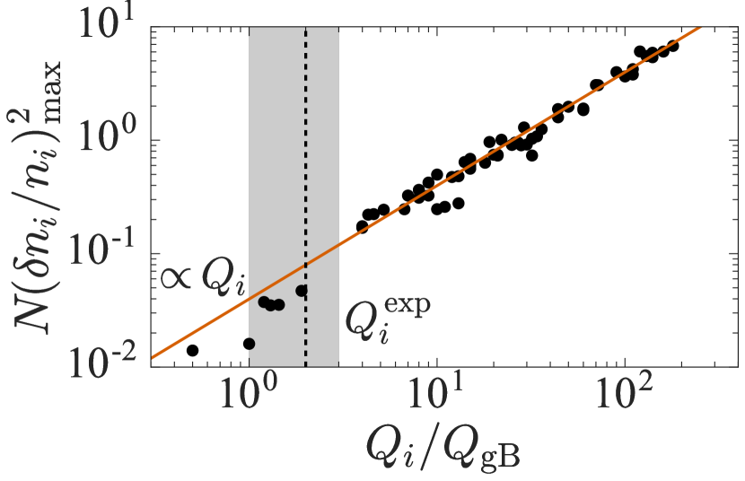
(b)

Figure 20: 20(a) Number of structures (defined as instance of the perturbed density with an amplitude above 75% of the maximum) versus $Q_{i}/Q_{\mathrm{gB}}$. It grows as $Q_{i}/Q_{\mathrm{gB}}$ increases up to and slightly beyond the experimental value $Q_{i}^{\exp}$. Eventually the volume is filled with structures and their number tends to a constant. The scaling $Q_{i}\propto N$ is shown for reference. 20(b) Confirmation of the scaling (18), where the red line indicates a line $\propto Q_{i}$. We note that simulations near marginality are relatively difficult to saturate leading to the low number of simulations around $Q_{i}^{\exp}$. However, the trend is still clear even for those simulations.

Figure 20(a) shows the results of the above analysis applied to our entire set of simulations: the number of structures $N$ with amplitudes above the 75^th percentile versus the ion heat flux $Q_{i}/Q_{\mathrm{gB}}$. As in figure 18, there are two distinct regimes: $N$ grows with $Q_{i}/Q_{\mathrm{gB}}$ until the structures have filled the simulation domain (which happens just above the experimental value of the flux), whereupon $N$ tends to a constant.

Taking figures 18 and 20(a) in combination, we have, roughly,

$$\frac{Q_{i}}{Q_{\mathrm{gB}}}\sim N{\quantity(\frac{\delta n_{i}}{n_{i}})}_{\max}^{2},$$ (18)

i.e., near the threshold, the turbulent heat flux increases because coherent structures become more numerous (but not more intense), whereas away from the threshold, it does so because the fluctuation amplitude increases (at a roughly constant number of structures). This relationship is confirmed by figure 20(b), where the scaling (18) is checked directly.

3.3.5 Shear due to zonal flows

In the conventional picture of the saturation mechanism of ITG-driven turbulence, zonal modes play a key role [85, 86, 67, 82, 87]. Zonal modes are fluctuations in the system with $k_{y}=k_{\parallel}=0$ and $k_{x}>0$, i.e., they have finite radial extent, but are poloidally symmetric. They are generated by nonlinear interactions in the system. Previous work [67] on the transition to turbulence in the case of $\gamma_{E}=0$ showed that near the turbulence threshold (approached by varying the equilibrium parameter $\kappa_{T}$), turbulence is regulated by strong zonal flows, which can cause an upshift in the critical $\kappa_{T}$ required for a saturated strongly turbulent state. However, in our system, the near-threshold cases the background flow shear plays an important role, and also has a suppressing effect on the turbulence.

Here, we investigate the relative importance of the mean shear and the shear resulting from the self-generated zonal flows. The shear due to the zonal flows $V^{\prime}_{\mathrm{ZF}}$ is calculated from (16) by considering only the poloidally symmetric component, that is

$$V^{\prime}_{\mathrm{ZF}}=\frac{c}{aB_{\mathrm{ref}}}\frac{q_{0}}{r_{0}}\frac{1}{|\nabla\alpha|}\partialderivative[2]{\varphi_{\mathrm{ZF}}}{x},$$ (19)

where $\alpha$ is the binormal coordinate, $\varphi_{\mathrm{ZF}}$ is the poloidally symmetric component of $\varphi$ and $V^{\prime}_{\mathrm{ZF}}$ is a function only of $t$ and $x$. To determine whether the zonal shear will dominate over the mean shear $\gamma_{E}$ we calculate the RMS value of the zonal shear, $\gamma_{\mathrm{ZF}}$:

$$\gamma_{\mathrm{ZF}}=\left<V^{\prime 2}_{\mathrm{ZF}}\right>^{1/2}_{t,x},$$ (20)

where $\left<{\cdots}\right>_{t,x}$ indicates an average over $t$ and $x$. We can now compare $\gamma_{\mathrm{ZF}}$ with $\gamma_{E}$ to determine their relative size as a function of our equilibrium parameters.

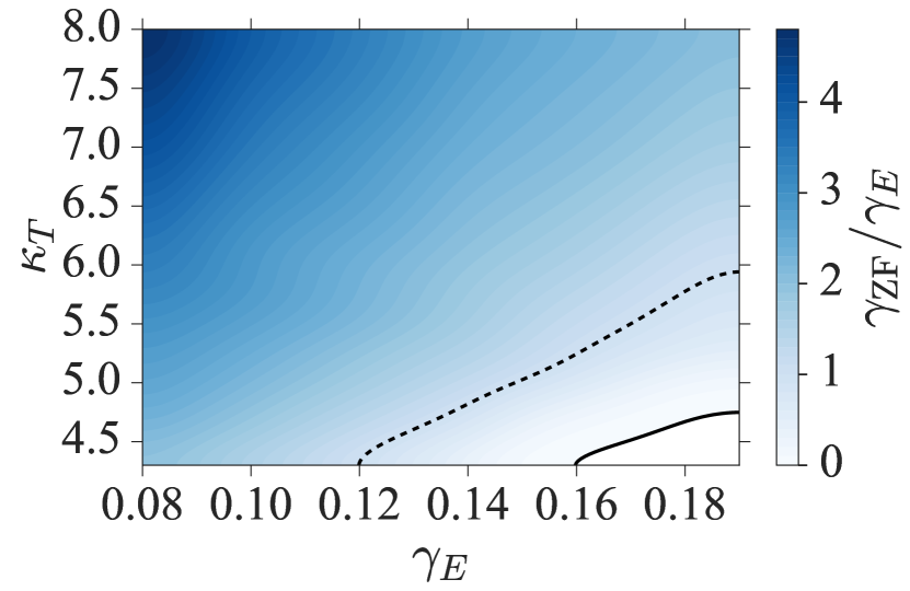
(a)

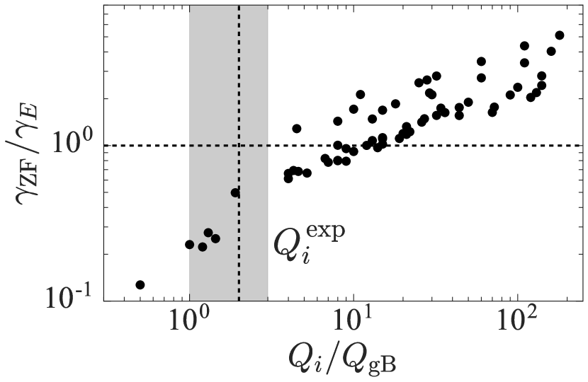
(b)

Figure 21: 21(a) The ratio of zonal shear to mean equilibrium flow shear $\gamma_{\mathrm{ZF}}/\gamma_{E}$ over the same range of $\kappa_{T}$ and $\gamma_{E}$ as shown in figure 5. The zonal shear and mean flow shear are comparable when $\gamma_{\mathrm{ZF}}/\gamma_{E}\sim 1$. The white region in the lower right-hand corner, separated by a solid line, indicates the region where there is no turbulence, i.e., $Q_{i}=0$ [see figure 5], and the dashed black line indicates $\gamma_{\mathrm{ZF}}/\gamma_{E}=1$. 21(b) $\gamma_{\mathrm{ZF}}/\gamma_{E}$ as a function of $Q_{i}/Q_{\mathrm{gB}}$. The vertical dashed line indicates the value of the experimental heat flux and the horizontal dashed line indicates $\gamma_{\mathrm{ZF}}/\gamma_{E}=1$.

Figure 21(a) shows the ratio of the zonal shear to the flow shear, $\gamma_{\mathrm{ZF}}/\gamma_{E}$, as a function of $\kappa_{T}$ and $\gamma_{E}$ over the same parameter range as shown in figure 5. The magnitudes of $\gamma_{\mathrm{ZF}}$ and $\gamma_{E}$ are comparable where $\gamma_{\mathrm{ZF}}/\gamma_{E}\sim 1$, which is indicated by the dashed line. We see that the regime in which $\gamma_{\mathrm{ZF}}$ and $\gamma_{E}$ become comparable occurs some distance away from the turbulence threshold (solid line). Therefore, close to the threshold (small $\gamma_{\mathrm{ZF}}/\gamma_{E}$), we expect the shear due to the background flow to dominate, while far from the threshold (large $\gamma_{\mathrm{ZF}}/\gamma_{E}$), we expect the shear due to the zonal flows to dominate.

Figure 21(a) suggests that the change in $\gamma_{\mathrm{ZF}}/\gamma_{E}$ is effectively a function of the distance from the turbulence threshold. Figure 21(b) shows this dependence explicitly: $\gamma_{\mathrm{ZF}}/\gamma_{E}$ as a function of $Q_{i}/Q_{\mathrm{gB}}$. The vertical dashed line indicates $Q_{i}^{\exp}/Q_{\mathrm{gB}}$ and we see that $\gamma_{\mathrm{ZF}}/\gamma_{E}$ is quite small at this value. This suggests that zonal shear plays a weaker role than $\gamma_{E}$ in regulating experimentally relevant turbulence for this MAST configuration. Therefore, near-threshold and far-from-threshold turbulent states are distinguished by whether it is the mean or the zonal shear that plays a dominant role. Far from the threshold, the turbulence is likely similar to conventional ITG-driven turbulence in the absence of background flow shear. This is supported by figure 22, which shows $\gamma_{\mathrm{ZF}}$ as a function of $\gamma_{E}$. We see that for low $\gamma_{E}$ and/or high $\kappa_{T}$ (i.e. for cases far from the threshold), $\gamma_{\mathrm{ZF}}$ is approximately independent of $\gamma_{E}$ and close to the value that it takes at $\gamma_{E}=0$.

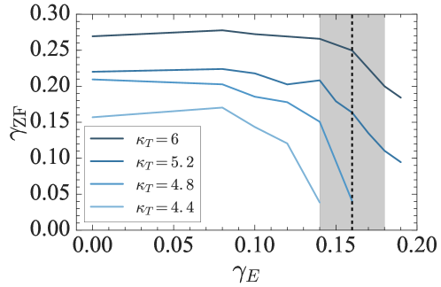
Figure 22: Zonal shear $\gamma_{\mathrm{ZF}}$ as a function of background flow shear $\gamma_{E}$ showing that zonal shear is comparable between low $\gamma_{E}$ (high $Q_{i}/Q_{\mathrm{gB}}$) cases and $\gamma_{E}=0$ cases.

3.3.6 Summary

In summary, we can describe the behaviour of the MAST turbulence that we studied as follows. For equilibrium parameters near the turbulence threshold (including for cases that match the experiment), the density and temperature fluctuations (and hence the heat flux) are concentrated in long-lived, intense coherent structures. As the equilibrium parameters $(\kappa_{T},\gamma_{E})$ depart slightly from their critical values into the more strongly driven regime, the number of the coherent structures increases rapidly while their amplitude stays roughly constant (in contrast to the conventional supercritical turbulence, where the amplitude increases with $\kappa_{T}$). Increasing $\kappa_{T}$ or decreasing $\gamma_{E}$ further leads to the structures filling the simulation domain and any further increase in the heat flux is caused by an increase in fluctuation amplitude. The latter regime is similar to the conventional plasma turbulence, where zonal flows are the dominant mechanism for regulating turbulence. In contrast, we have demonstrated that in the near-threshold cases, the zonal shear is small compared to the mean flow shear and so is unlikely to matter.

4 Correlation analysis and comparison with BES

In the previous section, we used nonlinear simulations to demonstrate the complicated nature of the MAST turbulence that we are studying, in particular the details of a subcritical transition to turbulence. In this section, we seek to establish the experimental relevance of our simulations using quantitative comparisons between the fluctuation fields predicted numerically and those measured by the BES diagnostic. We will review the BES diagnostic and experimental results (section 4.2) from Ref. [51], and then present two types of correlation analysis of our nonlinear simulations (the correlation-analysis techniques are described in appendix B). The first analysis will be of GS2 density fluctuations with a “synthetic BES diagnostic” applied to simulate what would be measured by a real BES diagnostic (section 4.3). We will consider the results from nonlinear simulations with values of $(\kappa_{T},\gamma_{E})$ within the experimental-uncertainty range and compare them with the experimental results. The second analysis will be of the raw GS2 density fluctuations, both within the experimental-uncertainty range and, as a function of $Q_{i}/Q_{\mathrm{gB}}$, for our entire parameter scan (section 4.4). In this latter case we will emphasise the extent to which it is the distance from the turbulence threshold rather than individual values of $\kappa_{T}$ or $\gamma_{E}$ that determines the statistical characteristics of the density fluctuations.

4.1 Beam emission spectroscopy diagnostic

Turbulent eddies in tokamak plasmas are anisotropic due to the strong background magnetic field. In the parallel direction, turbulent eddies have a length scale comparable to the system size, which in a torus is the connection length $\pi qR$ [88], i.e., $l_{\parallel}\sim\pi qR$ ($\approx 6$ m for MAST). In the direction perpendicular to the magnetic field, ITG-unstable turbulent structures have a typical length scale of the order of the ion gyroradius $l_{\perp}\sim\rho_{i}\sim 1$ cm. Therefore, in the plane perpendicular to the magnetic field, we are interested in two-dimensional measurements of fluctuating quantities at approximately the scale of $\rho_{i}$. Beam emission spectroscopy is a diagnostic technique that was developed to address this need. Specifically, the BES diagnostic on MAST [42, 43] is designed to measure ion-scale density fluctuations in a radial-poloidal plane. Density fluctuations are inferred from D_α emission produced by the NBI beam as it penetrates the plasma. The measured fluctuating intensity of the D_α emission is proportional to the local plasma density at the corresponding viewing location, and the two quantities are related via point-spread functions (PSFs) [47, 51, 49]. The PSFs depend on the magnetic equilibrium, beam parameters, viewing location, and plasma profiles and as a result, have to be calculated explicitly for each measurement [47].

Recent work [49], based on a subset of simulations presented here, has shown that the PSFs play an important role in the measurement of turbulence and that the precise form that they take determines a lower bound on the BES resolution as well as affecting the measurement of the turbulent structures and density fluctuation levels – effects that we will also consider in this work. For further details on the MAST BES system the reader is referred to Refs. [42, 43, 47] and, for a detailed study of the effect of PSFs on the measurement of turbulent structures, to Ref. [49].

4.2 Experimental BES results

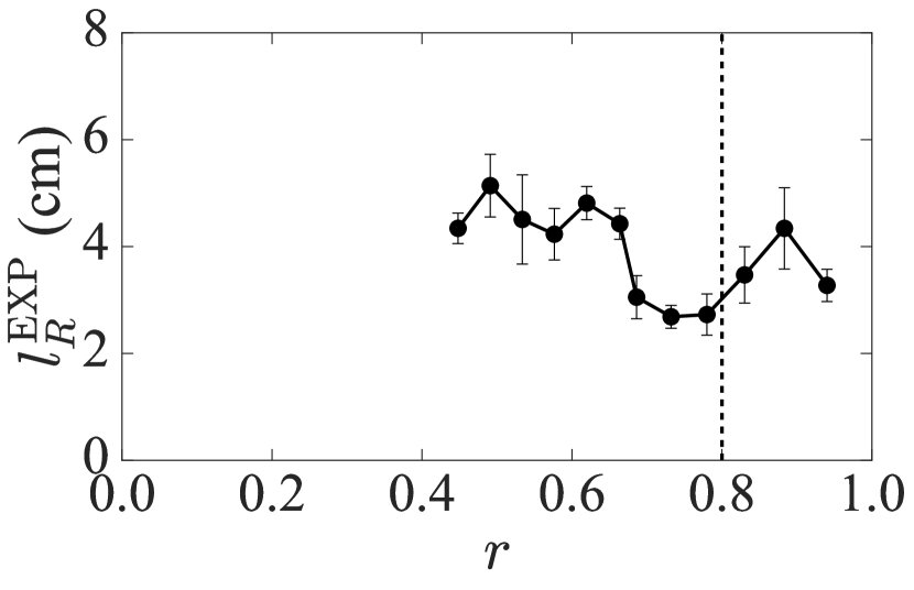
(a)

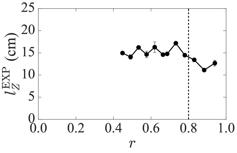
(b)

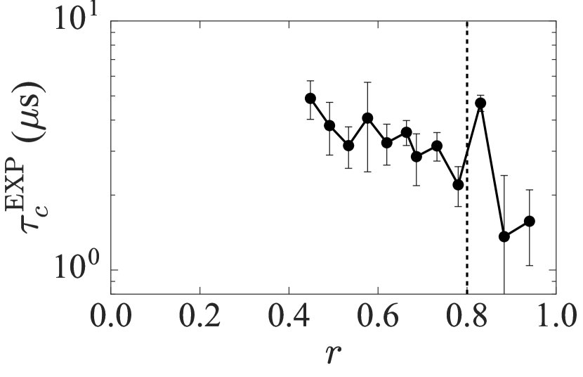
(c)

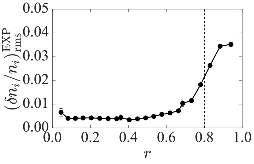
(d)

Figure 23: Results of the correlation analysis of BES data from MAST discharges #27272, #27268, and #27274 combined to give correlation properties of the turbulence as functions of $r=D/2a$: 23(a) radial correlation length $l_{R}^{\mathrm{EXP}}$, 23(b) poloidal correlation length $l_{Z}^{\mathrm{EXP}}$, 23(c) correlation time $\tau_{c}^{\mathrm{EXP}}$, and 23(d) RMS fluctuation amplitude $\quantity(\delta n_{i}/n_{i})^{\,\mathrm{EXP}}_{\mathrm{rms}}$. These quantities are defined in appendix B. Turbulence was suppressed for $r\lesssim 0.4$. The vertical dashed line indicates the radius corresponding to the local equilibrium configurations for which we performed our simulations.

Before applying the correlation analysis to our simulations, we review the experimental results from MAST discharge #27274 first presented in Ref. [51], to which we will be comparing our own calculation. As discussed in section 2.2, MAST discharge #27274 forms part of a set of three discharges, which together allowed measurement of turbulence correlation properties over the whole outer radius. Figure 23 shows the experimental results obtained for the radial correlation length $l_{R}^{\mathrm{EXP}}$, the poloidal correlation length $l_{Z}^{\mathrm{EXP}}$, the correlation time $\tau_{c}^{\mathrm{EXP}}$, and the RMS density fluctuations ${\quantity(\delta n_{i}/n_{i})}^{\mathrm{EXP}}_{\mathrm{rms}}$ as functions of $r=D/2a$. The vertical dashed line in each plot indicates the radius at which our simulations were done and the corresponding values of the correlation parameters. These target experimental values are (after interpolating between the experimental data points):

$$\begin{split}l_{R}^{\mathrm{EXP}}&=3\pm 0.4~{}\mathrm{cm},\\ l_{Z}^{\mathrm{EXP}}&=14.06\pm 0.09~{}\mathrm{cm},\\ \tau_{c}^{\mathrm{EXP}}&=3.2\pm 0.4~{}\mu\mathrm{s},\\ {\quantity(\frac{\delta n_{i}}{n_{i}})}^{\mathrm{EXP}}_{\mathrm{rms}}&=0.0214\pm 0.0006.\end{split}$$ (21)

We will be comparing the correlation parameters calculated from our simulations in the following sections to those in (21).

4.3 Correlation analysis with synthetic diagnostic

In order to compare our simulated density field with the BES-measured ones, a number of data transformations were necessary. We mapped our density fluctuations “measured” in the outboard midplane (at $\theta=0$) from GS2 $(x,y)$ coordinates onto a poloidal $(R,Z)$-plane and also transformed them from the rotating plasma frame, the frame in which our simulations were performed, to the laboratory frame, as explained in appendix C. We then applied a synthetic diagnostic to our density fluctuations, including the point-spread functions (described in section 4.1), which models instrumentation effects and atomic physics, adds artificial noise similar to that found in the experiment, and maps the density-fluctuation field onto an $8\times 4$ grid similar to the arrangement of BES channels. An important feature of the analysis of experimental data is the application of a filter to remove high-energy radiation present in the experiment. We have included this filter for consistency with experimental measurements. The results without this filter are presented in appendix E.

Figure 24 shows the radial correlation length $l_{R}^{\,\mathrm{SYNTH}}$, poloidal correlation length $l_{Z}^{\,\mathrm{SYNTH}}$, correlation time $\tau_{c}^{\,\mathrm{SYNTH}}$, and RMS density fluctuation $\quantity(\delta n_{i}/n_{i})^{\,\mathrm{SYNTH}}_{\mathrm{rms}}$ calculated from our simulations with the synthetic diagnostic applied using the correlation analysis described in appendix B. The errors in the correlation parameters shown in figure 24, and elsewhere, are determined from the fitting procedures described in appendix B. We expect these values to agree with the experimentally measured correlation parameters in (21) because the equilibrium parameters $\kappa_{T}$ and $\gamma_{E}$ at which the results shown in figure 24 were obtained are strictly within the experimental-uncertainty range of these parameters. The dashed lines and shaded areas in figure 24 indicate the experimental values and associated errors given in (21). The circled points indicate the simulations that matched the experimental level of heat flux (listed in table 2).

(a)

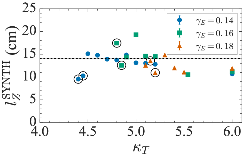
(b)

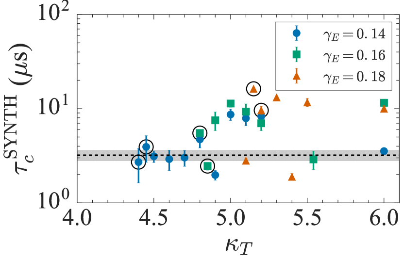
(c)

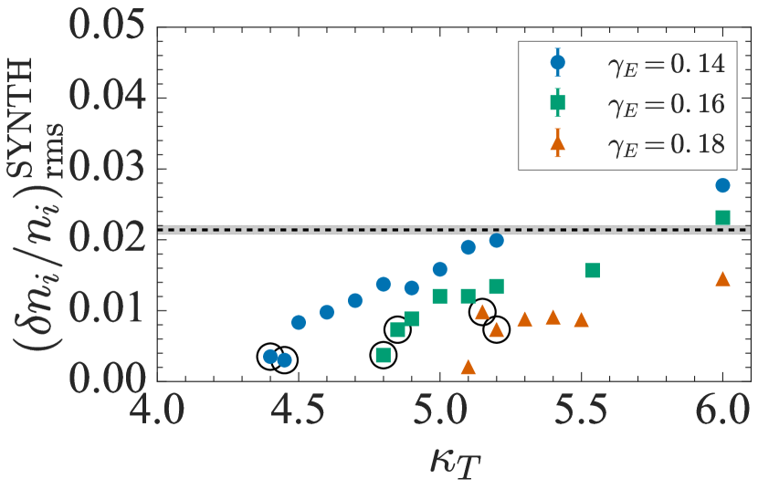
(d)

Figure 24: Comparison of correlation parameters obtained via synthetic BES measurements of GS2-simulated density field: 24(a) radial correlation length $l_{R}^{\mathrm{SYNTH}}$, 24(b) poloidal correlation length $l_{Z}^{\mathrm{SYNTH}}$, 24(c) correlation time $\tau_{c}^{\mathrm{SYNTH}}$, and 24(d) RMS fluctuation amplitude $\quantity(\delta n_{i}/n_{i})^{\,\mathrm{SYNTH}}_{\mathrm{rms}}$ as functions of $\kappa_{T}$ and for several values of $\gamma_{E}$ within experimental uncertainty. The circled points indicate the simulations match the experimental heat flux, given in table 2. The dashed lines indicate the experimental values and the shaded areas the associated error at $r=0.8$ obtained from interpolating between experimental measurements seen in figure 23, which correspond to the local equilibrium configuration studied in these simulations.

Examining figure 24(a), we see that the values of $l_{R}^{\,\mathrm{SYNTH}}$ are clustered around $2$ cm and below the experimental BES measurement $l_{R}^{\,\mathrm{EXP}}=3\pm 0.4$ cm. The approximate resolution limit in the radial and poloidal directions is $\sim 2$ cm, the physical separation between BES channels [42]. More recent work studying the measurement effect of the PSFs, concluded that the radial resolution limit can be between $2$ and $4$ cm depending on the orientation of the PSFs for a given configuration [49]. It is, therefore, likely that the results shown in figure 24(a) simply confirm the radial resolution limit of the experimental analysis and the true value of $l_{R}$ may be lower than 2 cm (as suggested in appendix B.1). We will confirm this in section 4.4, where we consider the correlation properties of the raw GS2 density fluctuations.

Figures 24(b)–24(d) show $l_{Z}^{\,\mathrm{SYNTH}}=$ $10$–$15$ cm, $\tau_{c}^{\,\mathrm{SYNTH}}=$ $2$–$15$ $\mu$s, and $\quantity(\delta n_{i}/n_{i})^{\,\mathrm{SYNTH}}_{\mathrm{rms}}\sim$ $0.005$–$0.03$. We see that these values match experimental measurements (21) for certain combinations of $\kappa_{T}$ and $\gamma_{E}$. The values of $l_{Z}^{\,\mathrm{SYNTH}}$ are scattered around the experimental value $l_{Z}^{\,\mathrm{EXP}}=14.06\pm 0.09$ cm, showing no clear trend. While none of the cases that match the experimental heat flux (circled cases) match $l_{Z}^{\,\mathrm{EXP}}$, there are several simulations within the experimental-uncertainty ranges of $\kappa_{T}$ and $\gamma_{E}$ that do. Similarly, there are several values of $\tau_{c}^{\,\mathrm{SYNTH}}$ that also match $\tau_{c}^{\,\mathrm{EXP}}$, including two cases that match the experimental level of heat flux. This is a considerable improvement over previous nonlinear gyrokinetic simulations of this MAST discharge [51], which overpredicted $\tau_{c}^{\,\mathrm{SYNTH}}$ by two orders of magnitude.

Examining figure 24(d), we see that $\quantity(\delta n_{i}/n_{i})^{\,\mathrm{SYNTH}}_{\mathrm{rms}}$ increases with increasing $\kappa_{T}$ or decreasing $\gamma_{E}$ and that increasing $\gamma_{E}$ leads to a increase in the value of $\kappa_{T}$ required to achieve the same $\quantity(\delta n_{i}/n_{i})^{\,\mathrm{SYNTH}}_{\mathrm{rms}}$. The latter trend is consistent with figure 7(a), which showed that increasing $\gamma_{E}$ shifted the nonlinear turbulence threshold to higher $\kappa_{T}$. While figure 24(d) shows that there is agreement between $\quantity(\delta n_{i}/n_{i})^{\,\mathrm{SYNTH}}_{\mathrm{rms}}$ and $\quantity(\delta n_{i}/n_{i})^{\,\mathrm{EXP}}_{\mathrm{rms}}$ at certain combinations of $(\kappa_{T},\gamma_{E})$, we see that the circled cases, representing simulations that match the experimental heat flux, have values of $\quantity(\delta n_{i}/n_{i})^{\,\mathrm{SYNTH}}_{\mathrm{rms}}$ well below $\quantity(\delta n_{i}/n_{i})^{\,\mathrm{EXP}}_{\mathrm{rms}}$.

We conclude from the above results that local gyrokinetic simulations are a reasonable approximation to the experimental turbulence. We showed that $l_{Z}^{\,\mathrm{SYNTH}}$ and $\tau_{c}^{\,\mathrm{SYNTH}}$ showed reasonable agreement with the experimental measurements within the experimental-uncertainty ranges, while there was a discrepancy in the predictions of $l_{R}^{\,\mathrm{EXP}}$ and $\quantity(\delta n_{i}/n_{i})^{\,\mathrm{EXP}}_{\mathrm{rms}}$. Thus, at least as far as BES measurements are concerned, the experimental turbulence and the synthetic turbulence are comparable.

One phenomenon that was not present in our simulations but is present in the experiment is high-energy radiation (e.g., neutron, gamma ray, or hard X-ray) impinging on the BES detectors. These photons cause high-amplitude spikes in the time series, which are typically confined to a single detector channel and, therefore, uncorrelated with other channels. These radiation spikes then give rise to large auto-correlations at zero time delay, which are unrelated to the turbulent field that is being measured. A numerical “spike filter” is normally used to remove radiation spikes by identifying changes above a certain threshold between one time point and the next, and replacing the high-intensity value with the value of a neighbouring point [43, 89]. This “spike filter” is an important component of the experimental analysis of BES data and, while our simulations do not include spurious sources of radiation, we have included the “spike filter” in the analysis of our simulated density fluctuations for consistency with experimental analysis. The results without the “spike filter” are given in appendix E. These results show little difference to those with the “spike filter” except for the value of $l_{Z}$. We found that in some cases, fast-moving structures in the poloidal direction (especially the long-lived structures found in our simulations close to the turbulence threshold) were removed by the “spike” filter and, therefore, did not contribute to the poloidal correlation function, resulting in a drop in $l_{Z}$. This is an important caveat for a future programme of experimental detections of these structures. For a more detailed discussion, see appendix E.

4.4 Correlation analysis of raw GS2 data

Having considered the structure of turbulence processed through a synthetic BES diagnostic, we now want to investigate the raw GS2 density fluctuations, which will allow us to (i) study the (distorting) effect of the synthetic diagnostic, (ii) study the parallel correlations using GS2 data along the field line, and (iii) consider our entire parameter scan to understand how the structure of turbulence in MAST might change with the equilibrium parameters $\kappa_{T}$ and $\gamma_{E}$. This extends the previous analysis and comparison with simulations performed for this MAST discharge [51], which only considered the nominal equilibrium parameters and simulations with a synthetic diagnostic applied. The only operations applied here to the raw GS2 density-fluctuation field output are the transformation to the laboratory frame, as explained in appendix C.1, and the transformation from the GS2 parallel coordinate $\theta$ to the real-space coordinate $\lambda$, as explained in appendix C.3. Our perpendicular correlation analysis is performed over a square $(R,Z)$-plane $20\times 20$ cm² in size, located at the centre of our computational domain (see appendix C.2). We do this to analyse a region of similar size to that probed by the BES diagnostic and also to avoid the real-space remapping effect at the edges of the radial domain inherent to the GS2 implementation of flow shear (see appendix D).

4.4.1 Correlation parameters for cases within experimental-uncertainty range

We start by considering the correlation analysis results for simulations with values of $\kappa_{T}$ and $\gamma_{E}$ within the experimental-uncertainty range. Figure 25 shows the radial correlation length $l_{R}^{\mathrm{GS2}}$, the poloidal correlation length $l_{Z}^{\mathrm{GS2}}$, the correlation time $\tau_{c}^{\mathrm{GS2}}$, and the RMS density fluctuation ${\quantity(\delta n_{i}/n_{i})}^{\mathrm{GS2}}_{\mathrm{rms}}$ calculated for our GS2 density-fluctuation field. The results shown in figure 25 are for a range of values of $\kappa_{T}$ and for $\gamma_{E}=[0.14,0.16,0.18]$, with circled points describing the simulations that match the experimental value of the heat flux.

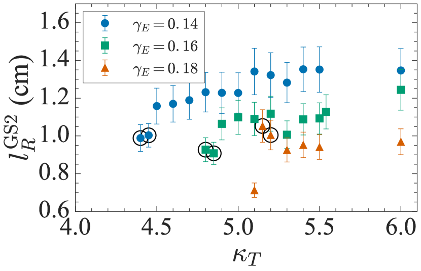
(a)

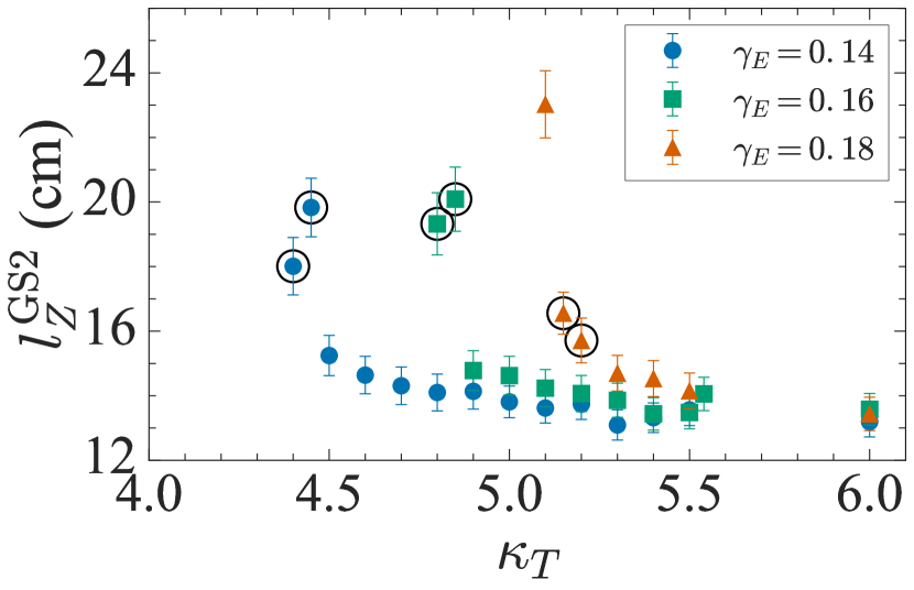
(b)

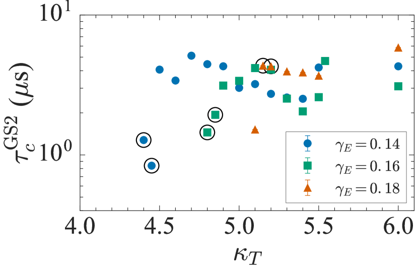
(c)

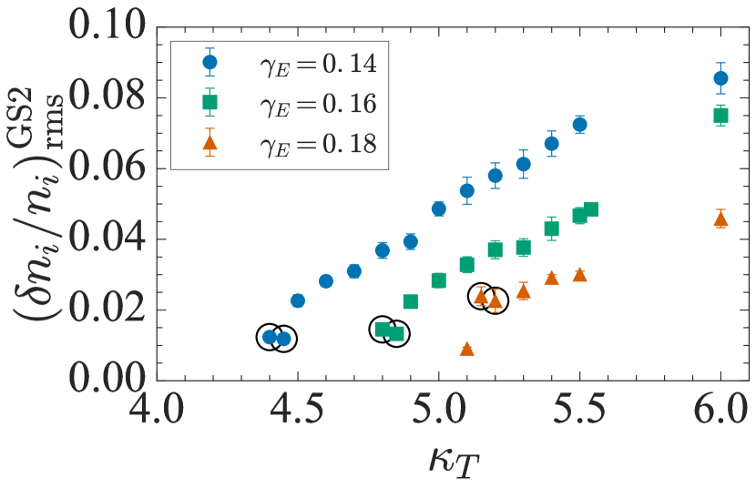
(d)

Figure 25: Correlation parameters calculated for raw GS2 density fluctuations for $(\kappa_{T},\gamma_{E})$ within the range of experimental uncertainty indicated in figure 5: 25(a) radial correlation length $l_{R}^{\mathrm{GS2}}$, 25(b) poloidal correlation length $l_{Z}^{\mathrm{GS2}}$ keeping $k_{y}$ fixed to $k_{y}=2\pi/l_{Z}$, 25(c) correlation time $\tau_{c}^{\mathrm{GS2}}$, and 25(d) RMS density fluctuations ${\quantity(\delta n_{i}/n_{i})}^{\mathrm{GS2}}_{\mathrm{rms}}$.

We find that the radial correlation length is $l_{R}^{\mathrm{GS2}}\sim$ $1$–$1.5$ cm, increasing with $\kappa_{T}$ and decreasing with $\gamma_{E}$. This suggests that $l_{R}^{\mathrm{GS2}}$ has a tendency to increase with $Q_{i}/Q_{\mathrm{gB}}$, as we will show explicitly later. In comparison with the synthetic-diagnostic results shown in figure 24(a), where $l_{R}^{\mathrm{SYNTH}}\sim 2$ cm, the true radial correlation length of the turbulence $l_{R}^{\mathrm{GS2}}$ is below $2$ cm and, therefore, below the resolution threshold of the BES diagnostic (discussed in section 4.3).

Figure 25(b) shows that the poloidal correlation length is $l_{Z}^{\mathrm{GS2}}\sim$ $13$–$20$ cm (to be compared with $l_{Z}^{SYNTH}=10$–$15$ cm), keeping the poloidal wavenumber $k_{Z}^{\mathrm{GS2}}$ fixed to $k_{Z}^{\mathrm{GS2}}=2\pi/l_{Z}^{\mathrm{GS2}}$ (giving $k_{Z}^{\mathrm{GS2}}\sim$ $30$–$50$ m^-1). We see that $l_{Z}^{\mathrm{GS2}}$ decreases rapidly as $\kappa_{T}$ is increased from its value at the turbulence threshold. The correlation time [figure 25(c)] is in the range $\tau_{c}^{\mathrm{GS2}}\sim$ $1$–$6$ $\mu$s. Finally, figure 25(d) shows that ${\quantity(\delta n_{i}/n_{i})}^{\mathrm{GS2}}_{\mathrm{rms}}\sim$ $0.01$–$0.08$ and increases with increasing $\kappa_{T}$ or decreasing $\gamma_{E}$, i.e., has an upward tendency as the heat flux increases.

4.4.2 Comparisons between experimental and GS2 correlation properties

We have presented the correlation parameters measured (i) by the BES diagnostic in section 4.2, (ii) from GS2 density fluctuations with the synthetic diagnostic applied in section 4.3, and (iii) from the raw GS2 density fluctuations. We show the results from all these analyses in table 3. We can thus summarise the comparison between simulation results and experimental measurements as follows. Comparing the results of the correlation analysis of the GS2 density fluctuations (“SYNTH” and “GS2” in table 3) with the experimental measurements (“EXP”), we see that all the experimental values, except for the radial correlation length $l_{R}$, fall within the ranges found for the simulation results. This is particularly important in the case of $\tau_{c}$, which was significantly overestimated in the previous modelling effort for this MAST discharge [51]. It is clear that the correlation parameters vary with the equilibrium parameters and there is no single simulation, i.e., no single combination of $(\kappa_{T},\gamma_{E})$, that perfectly matches the BES measurements in all four parameters (see figure 25).

Table 3: Summary of results for the correlation parameters $l_{R}$, $l_{Z}$, $\tau_{c}$, and $(\delta n_{i}/n_{i})_{\mathrm{rms}}$ from experimental BES measurements (EXP), from the correlation analysis of GS2 density fluctuations with synthetic diagnostic applied (SYNTH; using an identical correlation analysis to that used on the BES data), and from the correlation analysis of raw GS2 density fluctuations (GS2).

Parameter	EXP	SYNTH	GS2
$l_{R}$ (cm)	$3\pm 0.4$	1.5–2.5	1–1.5
$l_{Z}$ (cm)	$14.06\pm 0.09$	10–15	13–20
$\tau_{c}$ ($\mu$s)	$3.2\pm 0.4$	2–15	1–6
$(\delta n_{i}/n_{i})_{\mathrm{rms}}$	$0.0214\pm 0.0006$	0.005–0.03	0.01–0.08

Considering the difference between the GS2 density fluctuations with (SYNTH) and without (GS2) the synthetic diagnostic gives us an indication of the effect of the PSFs on the measurement of turbulence correlation properties. Given that the value of $l_{R}$ measured from the raw GS2 density fluctuations is below the approximate resolution threshold, it is unclear what effect the PSFs have on the radial correlation length $l_{R}$. We see from table 3 that the ranges of values of the poloidal correlation length $l_{Z}$ are comparable in the SYNTH and GS2 cases. However, figure 24(b) shows that, with the synthetic diagnostic applied, there are not the clear trends with $\kappa_{T}$ that we see in figure 25(b). This may be because the limited poloidal resolution, while sufficient to resolve the measured correlation lengths, is not sensitive enough to recover the trend of decreasing $l_{Z}$ with $\kappa_{T}$ seen in figure 25(b). The measurement of the correlation time $\tau_{c}$ is, again, less certain in the case of the correlation analysis of density fluctuations with a synthetic diagnostic applied, but there is reasonable agreement with the correlation time measured from the raw GS2 density fluctuations. Finally, the application of the synthetic diagnostic leads to a reduction of roughly $50$% of the RMS fluctuation amplitude, i.e., from ${(\delta n_{i}/n_{i})}^{\mathrm{GS2}}_{\mathrm{rms}}\sim$ $0.01$–$0.08$ for the raw density fluctuations to ${(\delta n_{i}/n_{i})}^{\mathrm{SYNTH}}_{\mathrm{rms}}~{}\sim$ $0.005$–$0.03$. This observation is consistent with a recent detailed analysis [49] of the effect of PSFs on the measurement of MAST turbulence using a subset of GS2 simulations reported here.

4.4.3 Poloidal and parallel correlation parameters

We now consider two further diagnostics, which were not available to us experimentally: poloidal and parallel correlation functions parametrised by the poloidal and parallel correlation lengths and wavenumbers (defined in appendix B) independently fitted as free parameters (although the poloidal correlation length was calculated previously in section 4.4.1, the resolution of the BES diagnostic necessitated fixing the poloidal wavenumber $k_{Z}$).

Figures 26(a) and 26(b) show the result of such fitting for the poloidal correlations: $l_{Z,\mathrm{free}}^{\mathrm{GS2}}$ and $k_{Z}^{\mathrm{GS2}}$ versus $\kappa_{T}$. As supported by figure 32 in appendix B.2, we see a roughly $50$% decrease in $l_{Z,\mathrm{free}}^{\mathrm{GS2}}$ compared to $l_{Z}^{\mathrm{GS2}}$ [figure 25(b)], from $13$–$20$ cm to $7$–$10$ cm, again decreasing as $\kappa_{T}$ increases or $\gamma_{E}$ decreases. Surprisingly, the value of $k_{Z,\mathrm{free}}^{\mathrm{GS2}}$ is still in the $35$–$45$ m^-1 range – comparable to one obtained via the fitting procedure where $k_{Z}=2\pi/l_{Z}$. Regardless of the fitting method, figure 25(b) and figure 26(a) show a similar dependence of $l_{Z}$ on $\kappa_{T}$ and $\gamma_{E}$.

The results of the parallel correlation analysis, given in figure 26(c) and 26(d), are the values $l_{\parallel}^{\mathrm{GS2}}$ and $k_{\parallel}^{\mathrm{GS2}}$ versus $\kappa_{T}$ and $\gamma_{E}$. We see that $l_{\parallel}^{\mathrm{GS2}}\sim$ $6$–$12$ m and decreases with increasing $\kappa_{T}$ and decreasing $\gamma_{E}$. Based on this measurement of the parallel correlation length, it is clear that the turbulence is highly anisotropic, i.e., $l_{\parallel}\gg l_{\perp}$, as it is expected to be [40].

Using the measurement of $l_{\parallel}^{\mathrm{GS2}}$, we can return to, and confirm, the assumption upon which the calculation of $\tau_{c}$ depends. Namely, in appendix B.3, we assume that reliably estimating the correlation time requires that the temporal decorrelation be dominant over effects due to the finite parallel correlation length [condition (28)]. Using the value of $l_{\parallel}$ reported above, we estimate $l_{\parallel}\cos\vartheta/u_{\phi}\sim$ $80$–$160$ $\mu$s, where we have used the experimental parameters $R=1.32$ m, $\omega=4.71\times 10^{4}$ $\mathrm{s}^{-1}$, and $\vartheta\approx 0.6$. This confirms that the values of $\tau_{c}$ summarised in table 3 are smaller than $l_{\parallel}\cos\vartheta/u_{\phi}$ by more than an order of magnitude and that our time correlation analysis is valid in this MAST configuration.

Currently the BES diagnostic on MAST is not capable of determining both $l_{Z}$ and $k_{Z}$, but the above estimates may be used for future comparisons between experimental measurements and numerical results if higher-resolution BES measurements become available. Similarly, there is currently no diagnostic on MAST capable of measuring the parallel correlation length, but our estimates may guide future attempts at designing diagnostics to measure it.

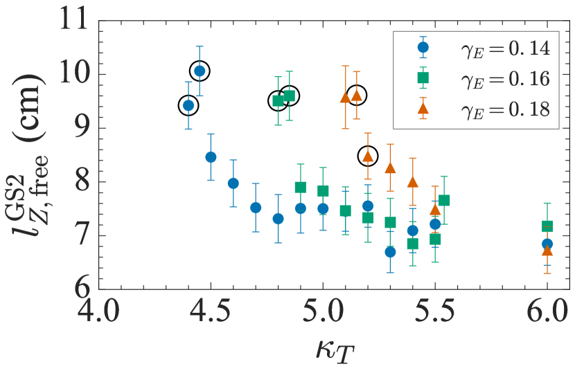
(a)

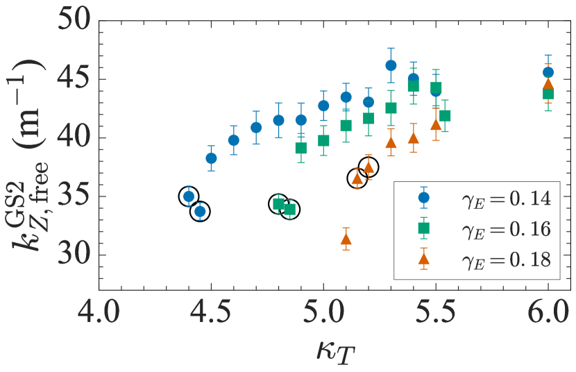
(b)

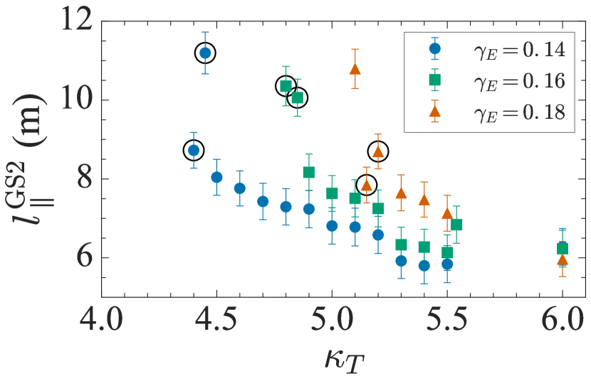
(c)

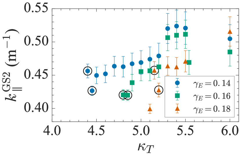
(d)

Figure 26: Correlation parameters calculated for raw GS2 density fluctuations for $(\kappa_{T},\gamma_{E})$ within the range of experimental uncertainty indicated in figure 5: 26(a) poloidal correlation length $l_{Z,\mathrm{free}}^{\mathrm{GS2}}$ with $k_{y}$ as a free fitting parameter, 26(b) poloidal wavenumber $k_{Z,\mathrm{free}}^{\mathrm{GS2}}$ (section B.2), 26(c) parallel correlation length $l_{\parallel}^{\mathrm{GS2}}$, and 26(d) parallel wavenumber $k_{\parallel}^{\mathrm{GS2}}$ (section B.4).

4.4.4 Comparison between linear and nonlinear time scales

With the knowledge of the correlation parameters, we can return to the comparison of the transient-growth time $t_{0}$ and nonlinear time $\tau_{\mathrm{NL}}$ discussed in section 3.2. In particular, we want to determine one of the two conditions for the onset of subcritical turbulence [equation (13)] proposed in [35]. We also want to compare $\tau_{\mathrm{NL}}$ with the correlation time of the turbulence $\tau_{c}$; we then discuss the corresponding experimental results in [51].

The non-zonal nonlinear interaction time is estimated to be [48]:

$$\tau_{\mathrm{NL}}^{-1}=\frac{v_{\mathrm{th}i}\rho_{i}}{l_{R}l_{Z}}\frac{T_{e}}{T_{i}}\quantity(\frac{\delta n_{i}}{n_{i}})_{\mathrm{rms}},$$ (22)

where we have assumed $l_{Z}\approx l_{y}$ (where $l_{y}$ is the correlation length in the binormal direction as defined in [48]) because $l_{Z}=l_{y}\cos\vartheta$, where $\vartheta$ is the magnetic field pitch-angle, and $\cos\vartheta\sim 1$ for this magnetic equilibrium. The transient-growth time $t_{0}$ was calculated from linear simulations and plotted in figure 10, showing that, at ion scales, the longest transient growth occurred at $k_{y}\rho_{i}\sim 0.1$. Figure 27(a) shows $\tau_{\mathrm{NL}}^{\mathrm{GS2}}$ versus $t_{0}$ (at $k_{y}\rho_{i}=0.1$) for all simulations with $\gamma_{E}>0$, where the dashed line indicates $\tau_{\mathrm{NL}}^{\mathrm{GS2}}=t_{0}$. We see that the majority of simulations are below the line defined by $\tau_{\mathrm{NL}}^{\mathrm{GS2}}=t_{0}$, showing that at the very least the condition (13) is approximately satisfied in most turbulent states, i.e., that $t_{0}\gtrsim\tau_{\mathrm{NL}}$. The inverse relationship between $\tau_{\mathrm{NL}}$ and $t_{0}$ is explained simply: as the strength of the drive increases and we move away from the turbulence threshold, the growth time of the transient amplification increases, the nonlinear interaction becomes more vigorous, and so the nonlinear time goes down.

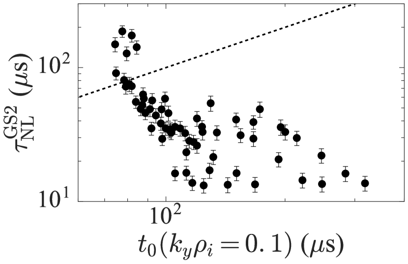
(a)

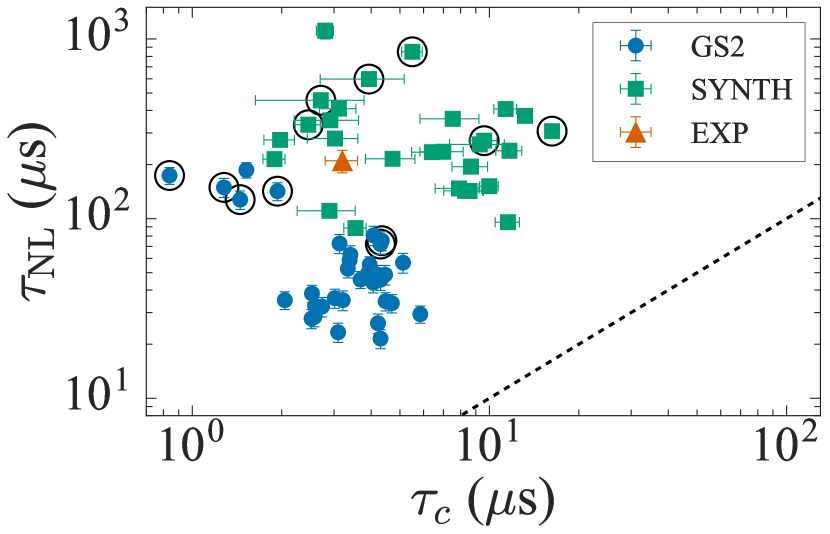
(b)

Figure 27: 27(a) Nonlinear interaction time of the raw GS2 density fluctuations $\tau_{\mathrm{NL}}^{\mathrm{GS2}}$, calculated using (22), versus the transient-growth time $t_{0}$, defined by (12). We have taken $t_{0}$ at $k_{y}\rho_{i}=0.1$, where $t_{0}$ is largest (see figure 10). We show here all simulations in our parameter scan with $\gamma_{E}>0$. 27(b) $\tau_{\mathrm{NL}}$ versus $\tau_{c}$ for the correlation parameters calculated from the raw GS2 density fluctuations (GS2), from density fluctuations with the synthetic diagnostic applied (SYNTH), and from experimental measurements (EXP). The cases shown are for values of $(\kappa_{T},\gamma_{E})$ within the experimental-uncertainty range and the circled simulations indicate the simulations that match the experimental heat flux. The dashed lines in each plot indicate where the time scales are equal.

Figure 27(b) shows $\tau_{\mathrm{NL}}$ versus $\tau_{c}$ for nonlinear simulations with values of $(\kappa_{T},\gamma_{E})$ within experimental uncertainty. The values of $\tau_{\mathrm{NL}}$ were calculated from correlation parameters of raw GS2 density fluctuations (GS2), from correlation parameters calculated from GS2 density fluctuations with a synthetic diagnostic applied (SYNTH), and from the experimental BES measurements at $r=0.8$ (EXP). The dashed line corresponds to $\tau_{\mathrm{NL}}=\tau_{c}$. First, we see that $\tau_{\mathrm{NL}}>\tau_{c}$ for both the GS2 and SYNTH cases, and for the experimental case (EXP). Secondly, $\tau_{\mathrm{NL}}$ for the raw GS2 density fluctuations tends to be below the experimental value, whereas the SYNTH cases are comparable. The results shown in figure 27(b) are consistent with the experimental results in [48, 51] that showed $\tau_{\mathrm{NL}}\gg\tau_{c}$ for this and other experimental cases.

It might appear strange that eddies would be able to interact nonlinearly with each other over a much longer time than it takes them to decorrelate. These results suggest either that (22) is a gross overestimate of the nonlinear interactions and/or that the value of $\tau_{c}$ that we measure from the turbulent density field captures some decorrelation process that is otherwise invisible to our synthetic diagnostic ([48] speculated that this might involve zonal flows). However, what is reassuring about these results is that GS2 simulations and BES measurements of turbulence in MAST appear to be consistent with each other in exhibiting this thus far unexplained feature.

4.4.5 Correlation parameters versus $Q_{i}/Q_{\mathrm{gB}}$

The correlation analysis results shown in figures 25 and 26, in particular $l_{Z}^{\mathrm{GS2}}$, $(\delta n_{i}/n_{i})^{\mathrm{GS2}}_{\mathrm{rms}}$, and $l_{\parallel}^{\mathrm{GS2}}$, exhibit similar trends versus $\kappa_{T}$ for different values of $\gamma_{E}$. As we showed in figure 5, increasing $\kappa_{T}$ or decreasing $\gamma_{E}$ effectively amounts to controlling the distance from the turbulence threshold. Furthermore, our investigations of the transition to turbulence (see [37] and section 3.2) and the effect of flow shear on its structure [89] suggest that the key determining factor is the distance from the threshold. This can be quantified by the ion heat flux $Q_{i}/Q_{\mathrm{gB}}$, which increases monotonically with this distance and can be interpreted as an order parameter for our system. Here we describe the results of our correlation analysis of raw GS2 density fluctuations recast as a function of this parameter.

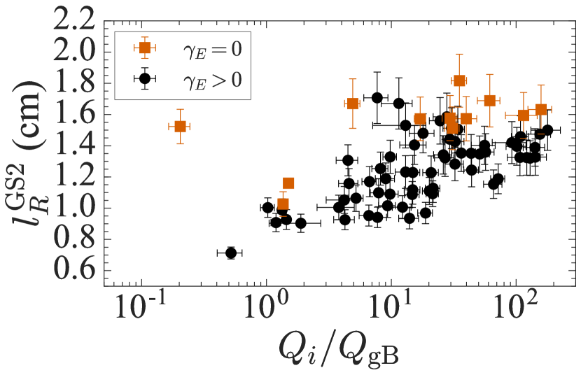
(a)

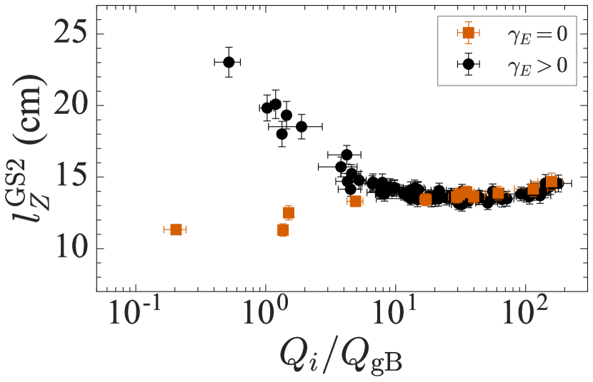
(b)

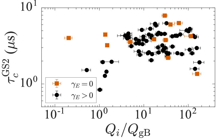
(c)

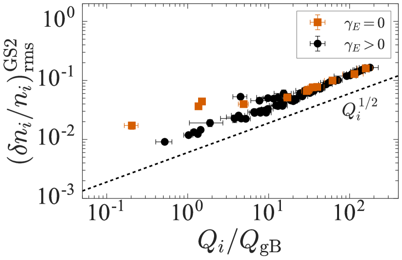
(d)

Figure 28: Correlation parameters as functions of $Q_{i}/Q_{\mathrm{gB}}$, calculated for raw GS2 density fluctuations for the entire parameter scan: 25(a) radial correlation length $l_{R}^{\mathrm{GS2}}$; 25(b) poloidal correlation length; $l_{Z}^{\mathrm{GS2}}$ keeping $k_{y}$ fixed to $k_{y}=2\pi/l_{Z}$; 25(c) correlation time $\tau_{c}^{\mathrm{GS2}}$; and 25(d) RMS density fluctuations $(\delta n_{i}/n_{i})^{\mathrm{GS2}}_{\mathrm{rms}}$, where the dashed line indicates the scaling (17).

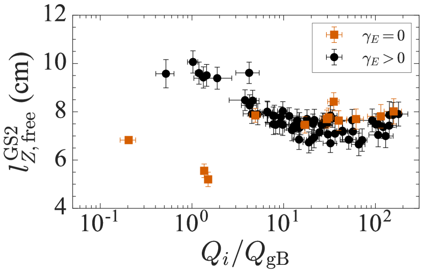
(a)

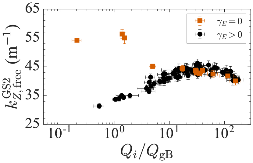
(b)

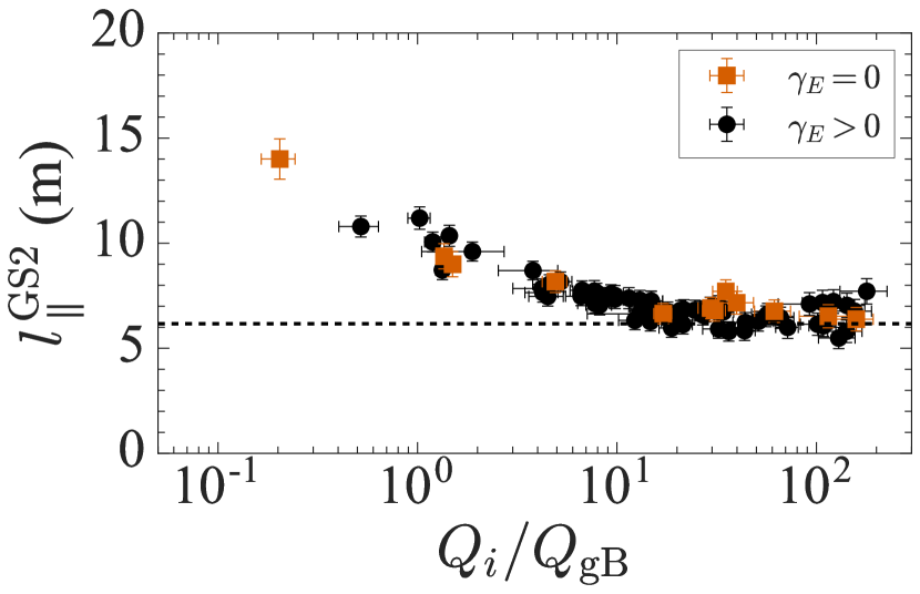
(c)

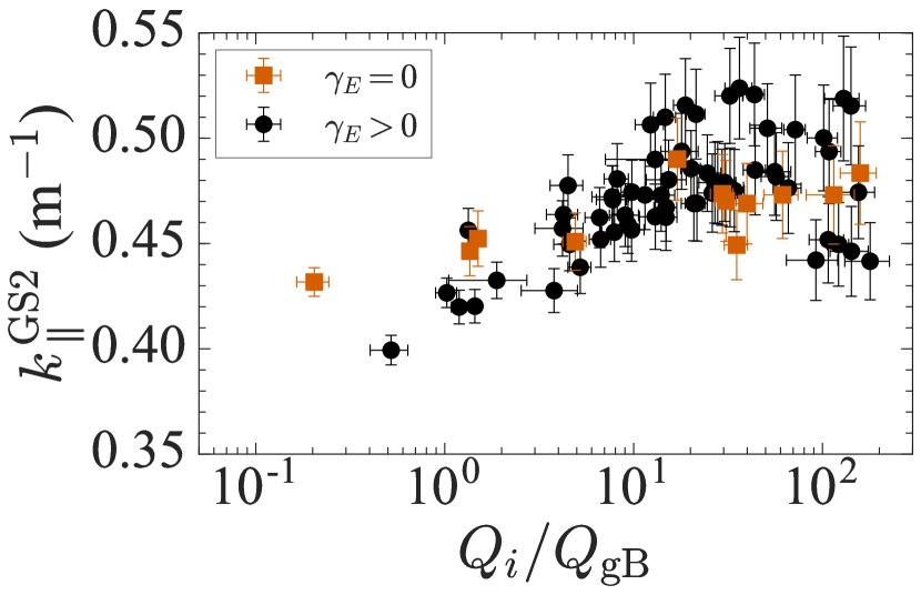
(d)

Figure 29: Correlation parameters as functions of $Q_{i}/Q_{\mathrm{gB}}$, calculated for raw GS2 density fluctuations for the entire parameter scan: 26(a) poloidal correlation length $l_{Z,\mathrm{free}}^{\mathrm{GS2}}$ with $k_{y}$ as a free fitting parameter and 26(b) poloidal wavenumber $k_{Z,\mathrm{free}}^{\mathrm{GS2}}$; 26(c) parallel correlation length $l_{\parallel}^{\mathrm{GS2}}$ and 26(d) parallel wavenumber $k_{\parallel}^{\mathrm{GS2}}$. The dashed line in 26(c) indicates a line of $l_{\parallel}\sim\pi qR$ (see main text and [88]).

Figures 28 and 29 show the correlation parameters from figures 25 and 26 as functions of $Q_{i}/Q_{\mathrm{gB}}$ for our entire parameter scan, including the cases with $\gamma_{E}=0$. These figures support the notion that it is distance from threshold that determines the structure of turbulence and characterise this structure for a realistic MAST configuration and for a large range of $Q_{i}/Q_{\mathrm{gB}}$. We start by discussing the $\gamma_{E}>0$ cases.

In figure 28(a), we see a roughly monotonic increase in the radial correlation length $l_{R}^{\mathrm{GS2}}$ with increasing $Q_{i}/Q_{\mathrm{gB}}$, this makes sense because the formation of larger radial structures is one way the turbulence can transport heat more effectively.

Figure 28(b) [along with figures 29(a) and 29(b)] shows the poloidal correlation length $l_{Z}^{\mathrm{GS2}}$ decreasing with increasing $Q_{i}/Q_{\mathrm{gB}}$. This is consistent with (17) (note that, according to figure 29(b), $k_{Z}$, and therefore $k_{y}$, increases as $l_{Z}$ decreases). Though figure 28(b) shows that $l_{Z}^{\mathrm{GS2}}$ decreases to roughly $14$ cm for $Q_{i}/Q_{\mathrm{gB}}\sim O(10)$, it starts increasing again for $Q_{i}/Q_{\mathrm{gB}}\sim O(100)$. This is perhaps in line with the theoretical and numerical estimates of the scaling of $l_{Z}$ far from the turbulence threshold predicting that $l_{Z}\sim q\kappa_{T}$ [88]. It stands to reason that at such high values of $Q_{i}/Q_{\mathrm{gB}}$, the system is entering a strongly driven regime, but further simulations at higher $\kappa_{T}$ are necessary to confirm whether our simulations adhere to the scaling predicted by [88].

The RMS density fluctuations $(\delta n_{i}/n_{i})^{\mathrm{GS2}}_{\mathrm{rms}}$ shown in figure 28(d) increase as $(Q_{i}/Q_{\mathrm{gB}})^{1/2}$ far from threshold, as expected from the scaling (17). However, in contrast to the results in figure 18, we do not see a flattening of $(\delta n_{i}/n_{i})^{\mathrm{GS2}}_{\mathrm{rms}}$ at low $Q_{i}/Q_{\mathrm{gB}}$ for $\gamma_{E}>0$ cases. This is due to the relatively little volume taken up by the coherent structures and, hence, their small contribution to the RMS value. We verified this by calculating the RMS density fluctuations while excluding varying numbers of the turbulence structures (near the threshold) and found that the RMS value did not change very much, confirming that for the cases near the threshold the RMS value is dominated by the low-amplitude density fluctuations.

Finally, in figure 29(c), we see that the parallel correlation length $l_{\parallel}^{\mathrm{GS2}}$ decreases towards a constant value as the system is taken away from the turbulence threshold. Theoretical and numerical estimates of $l_{\parallel}$ for strongly driven ITG turbulence [88] indeed predicted that $l_{\parallel}$ should be constant and proportional to the connection length, viz. $l_{\parallel}\sim\pi qR$. This estimate is indicated by the dashed line in figure 29(c) and shows reasonably good agreement with the data.

We have included both the cases for which $\gamma_{E}=0$ (red) and those with $\gamma_{E}>0$ (black) in figures 28 and 29 to highlight two important features of unsheared versus sheared turbulence previously discussed in section 3.3. First, close to the turbulence threshold, the cases with $\gamma_{E}=0$ represent a different regime of turbulence to those with $\gamma_{E}>0$. In particular, $l_{Z}^{\mathrm{GS2}}$ shown in figure 28(b) [as well as in figures 29(a) and 29(b)], shows an increasing trend for cases with $\gamma_{E}=0$: from $\sim 10$ cm near the turbulence threshold (which is significantly lower than the sheared case at the experimentally relevant $Q_{i}/Q_{\mathrm{gB}}$) to $\sim 15$ cm far away from the threshold. In contrast, $l_{Z}^{\mathrm{GS2}}$ in cases with $\gamma_{E}>0$ decreases from $\sim 23$ cm near marginality to $\sim 15$ cm far away from it, before starting to increase in a similar trend to the $\gamma_{E}=0$ cases. Furthermore, figure 28(c) shows that $\tau_{c}^{\mathrm{GS2}}$ predicted by $\gamma_{E}=0$ simulations stays roughly constant over a large range of $Q_{i}/Q_{\mathrm{gB}}$ whereas for $\gamma_{E}>0$ simulations, $\tau_{c}^{\mathrm{GS2}}$ diminishes rapidly for small $Q_{i}/Q_{\mathrm{gB}}$. Secondly, we see that far from the threshold, the $\gamma_{E}=0$ and $\gamma_{E}>0$ cases for all correlation parameters show the same dependence on $Q_{i}/Q_{\mathrm{gB}}$. This suggests that far from the threshold there is little difference between sheared and unsheared (by a background flow) turbulence.

The above two observations highlight an important finding of this work: close to the turbulence threshold, the background flow shear has a significant effect on the turbulence leading to reduced heat transport, whereas far from the threshold, the turbulence appears to be similar to the conventional ITG-driven turbulence in the absence of flow shear. This result is consistent with the results in section 3.3 and with the conclusions of the related work in Ref. [89], which argued a similar case in terms of the reflection (up-down) symmetry of the turbulence being broken by the flow shear close to the threshold but effectively restored far from it.

5 Conclusions

We have simulated the plasma microturbulence in an equilibrium configuration corresponding to MAST discharge #27274 using local gyrokinetic simulations and performed a systematic parameter scan in the ion temperature gradient length scale $\kappa_{T}$ and the flow shear $\gamma_{E}$. We demonstrated in section 3.1 that, within experimental uncertainty, our simulations reproduce the experimental ion heat flux, and that the experimentally measured equilibrium gradients lie close to the turbulence threshold inferred from the simulations. This is one of the first numerical demonstrations that a MAST plasma is close to the turbulence threshold. The parameter scan performed in this work has clearly shown that $\kappa_{T}$ and $\gamma_{E}$ are useful control parameters (and in particular, that experimental values of $\gamma_{E}$ do matter for the turbulent state), supporting several previous experimental and numerical studies [81, 8, 90, 24].

We showed in section 3.2 that the system is subcritical for all values of $\gamma_{E}>0$, i.e., in the linear approximation, perturbations grow only transiently before decaying, and in the nonlinear system, finite initial perturbations, which we assume are available in the experiment, are required in order to achieve a non-zero saturated state. Subcriticality is a defining feature of this system: for $\gamma_{E}>0$, even cases with the largest values of $\kappa_{T}$ that we considered required large initial perturbations to ignite turbulence. Using linear and nonlinear simulations, we have estimated the conditions necessary for the onset of subcritical turbulence: we require that maximum transient-amplification factor be $N_{\gamma,\max}\gtrsim 0.4$, and that the transient-growth time $t_{0}$ be approximately greater than the nonlinear interaction time, i.e., $t_{0}\gtrsim\tau_{\mathrm{NL}}$ (section 4.4.4). These conditions were comparable to those in previous work for simpler geometric configurations [35, 73]. Furthermore, we have showed that the linear dynamics do not change in any quantitatively obvious way as the turbulence threshold is passed, and so nonlinear simulations are essential in predicting the onset of subcritical turbulence and mapping out the turbulence threshold in the parameter space.

Our simulations have shown that, near the turbulence threshold, a previously unreported turbulent state exists in which fluctuation energy is concentrated into a few coherent, long-lived structures, which have a finite minimum amplitude (section 3.3.1). We have argued that this phenomenon is due to the subcriticality of the system, which cannot support arbitrarily small-amplitude perturbations (in contrast to supercritical turbulence). We have investigated the changes in the nature of these nonlinear structures by tracking the maximum fluctuation amplitude (section 3.3.3) and the number of structures (section 3.3.4) as we changed our equilibrium parameters, and have arrived at the following picture of the transition to turbulence. Near the turbulence threshold, the system is comprised of just a few finite-amplitude structures, which are not volume-filling. As the system is taken away from the turbulence threshold, the number of these structures increases (while their amplitude stays the same). Upon increasing in number sufficiently to fill the spatial simulation domain, they begin to increase in amplitude (at a roughly constant number of structures). They also become much less long-lived in time, presumably breaking up against each other as they overlap and interact. Interestingly, this scenario of evolution of our system as it is taken away from the turbulence threshold is reminiscent of the transition to subcritical turbulence via localised structures in pipe flows [91].

We have further shown that, in contrast to conventional ITG-driven turbulence regulated by zonal flows [67] (and their associated shear), in our system, close to the turbulence threshold, the shear due to the mean toroidal flow dominates over the shear due to the zonal flows (section 3.3.5). We have shown that the nominal experimental gradients lie close to the threshold, meaning that it is essential to include the background flow shear in simulations of MAST plasmas. Only reasonably far from the turbulence threshold do the zonal shear and the flow shear due to the background flow become comparable, and further still the turbulence becomes similar to ITG-driven turbulence in the absence of background flow shear (cf. [89]).

We have made quantitative comparisons between density fluctuations in our simulations and those measured by the MAST BES diagnostic [42, 43] (section 4). A correlation analysis [47] was previously performed on the measurements of density fluctuations from the BES diagnostic [51] (section 4.2), focusing on the following properties of the turbulence: the radial correlation length $l_{R}$, the poloidal correlation length $l_{Z}$, and the correlation time $\tau_{c}$. We have performed two types of correlation analysis on our simulated density fluctuations: one after applying a synthetic BES diagnostic (section 4.3), and one directly on the raw GS2-generated density fluctuations (section 4.4). We have compared these results to experimental measurements and found reasonable agreement of the correlation lengths and correlation time, except for the radial correlation length, which was predicted by us to be lower than the resolution limit of the BES diagnostic. Notably, the simulated and experimentally measured correlation times were in good agreement, unlike in previous global, gyrokinetic simulations of the same MAST discharge [51]. However, we showed that, for simulations that match the experimental heat flux, GS2 underpredicts the fluctuation amplitude [figure 24(d)], similar to previous studies comparing gyrokinetic turbulence to BES measurements [50, 53, 46, 55]. While a 10–20% increase in $\kappa_{T}$ (i.e., within experimental uncertainty) leads to turbulence that matches the fluctuation amplitude, it also leads to significantly higher transport than experimental levels. It is not clear as yet why GS2 (or other) codes systematically predict lower fluctuation amplitudes than observed experimentally.

Finally, we have argued that the nature of the turbulence is effectively a function of the distance from the turbulence threshold. We have quantified this distance from threshold by the magnitude of the ion heat flux $Q_{i}/Q_{\mathrm{gB}}$, and have shown that it is this quantity, rather than the specific values of the equilibrium parameters $\kappa_{T}$ and $\gamma_{E}$, that determines the properties of the turbulence. Throughout this work, we have presented our data as functions of the distance from threshold to highlight the two distinct nonlinear regimes that we have identified: close to the threshold, where coherent structures dominate the dynamics, and far from the threshold, where the turbulence appears to be similar to conventional strongly driven ITG turbulence in the absence of flow shear (e.g. [67, 32]). The experiment appears to be located at the boundary of these two regimes in parameter space. This suggests that this boundary is the most experimentally relevant one, as opposed to the boundary separating the laminar and turbulent states—the so-called “zero-turbulence manifold” [73].

Using the local gyrokinetic code GS2, we have been able to reproduce both the experimental heat flux and the quantitative measurements of turbulence obtained using the BES diagnostic. This should perhaps give some credence to the conclusion from the simulations that do not (yet) have direct experimental backing. More broadly, this should serve to increase one’s confidence in the future use of local gyrokinetic simulations in predicting turbulence and transport in high-aspect-ratio spherical tokamaks such as MAST.

A key open question that results from this study is of the experimental existence of the long-lived, coherent structures near the turbulence threshold. Recent work on this topic provided some tentative but encouraging indications that such a regime might manifest itself in terms of experimentally observed skewed probability distributions of density fluctuations [89]. More extensive analysis of MAST BES measurements, and indeed more BES measurements are needed in future to identify these structures, if they do indeed exist experimentally. While we have focused on the ion heat flux in this study, future work may strive to include other transport channels, such as electron heat flux, momentum, and particle transport. This will require computationally expensive multiscale gyrokinetic simulations and will also describe the fine-scale ETG turbulence that is likely responsible for the majority of the heat transport in this plasma. Resolving electron scales, as well as scales intermediate to the ion and electron scales, would also allow comparison with other fluctuation diagnostics, such as the recently installed Doppler backscattering diagnostic on MAST [92].

Appendix A Full parameter scan

Our parameter scan in the equilibrium parameters $\kappa_{T}$ and $\gamma_{E}$ covered approximately $\kappa_{T}\in[3.0,8.0]$ and $\gamma_{E}\in[0,0.19]$, and consisted of approximately 76 simulations. Figure 30 shows the parameter values of $\kappa_{T}$ and $\gamma_{E}$ that we simulated, and the associated ion heat flux $Q_{i}/Q_{\mathrm{gB}}$. To produce figure 5, we interpolated between the parameter values in figure 30.

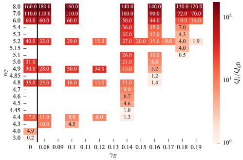
Figure 30: Ion heat flux $Q_{i}/Q_{\mathrm{gB}}$ as a function $\kappa_{T}$ and $\gamma_{E}$ explicitly showing the values of $Q_{i}/Q_{\mathrm{gB}}$. Figure 5 is a smoothed version of this figure.

Appendix B Correlation analysis

In this section, we give an overview of the correlation-analysis techniques used in Refs. [48, 51], which motivated the experimental comparisons presented in this paper. We will also present an alternative measurement of the poloidal correlation length $l_{Z}$, taking advantage of the increased resolution available in the poloidal direction from our simulations. While there is no experimental estimate of the parallel correlation length $l_{\parallel}$ available from the BES data, we are able to use the three-dimensional data available from GS2 to extend the correlation analysis to the parallel direction (see section 4.4.3).

The two-point spatio-temporal correlation function is defined to be

$$C(\Delta R,\Delta Z,\Delta\lambda,\Delta t)=\\ \frac{\left<\delta n_{i}/n_{i}(R,Z,\lambda,t)\delta n_{i}/n_{i}(R+\Delta R,Z+\Delta Z,\lambda+\Delta\lambda,t+\Delta t)\right>}{{\quantity[\left<{(\delta n_{i}/n_{i})}^{2}(R,Z,\lambda,t)\right>\left<{(\delta n_{i}/n_{i})}^{2}(R+\Delta R,Z+\Delta Z,\lambda+\Delta\lambda,t+\Delta t)\right>]}^{1/2}},$$ (23)

where $\delta n_{i}/n_{i}$ is the density-fluctuation field, which has a mean of zero, calculated by GS2 and $\Delta R$, $\Delta Z$, $\Delta\lambda$ are the radial, poloidal, and parallel point separations, $\Delta t$ is the time lag, and $\left<\ldots\right>$ is an ensemble average, viz. an average over all possible pairs of points with the same separation and time lag. Note that the ensemble averages in the plane perpendicular to the magnetic field are calculated at $\theta=0$, i.e., they are not averaged over $\theta$. This is because in the laboratory coordinate system, correlation properties vary strongly with $\theta$ owing to the twisting of the magnetic field lines. Here we wish to capture what occurs at the outboard midplane, which is the location of the BES diagnostic. Note also that we divide our data in the time domain into windows of $\sim 100$–$400$ $\mu$s, and calculate separate ensemble averages in each time window. We define the error bars on our correlation parameters by calculating variances between those values calculated over these time windows.

Instead of calculating the full correlation function (23), we will estimate individual correlation lengths and times (which are defined below) by performing one-dimensional correlation analyses separately in each direction, i.e., we calculate 1D versions of the correlation function (23), with respect to only one of its arguments. All of the representative correlation functions that are plotted in the sections that follow will be for the equilibrium parameters $(\kappa_{T},\gamma_{E})=(5.1,0.16)$ over a real-space domain of $20\times 20$ cm² (see figure 35).

B.1 Radial correlation length

The radial correlation length $l_{R}$ is estimated by fitting the correlation function $C(\Delta R,\Delta Z=0,\lambda(\theta=0),\Delta t=0)$ with a Gaussian function:

$$f_{R}(\Delta R)=\exp\quantity[-{\quantity(\frac{\Delta R}{l_{R}})}^{2}].$$ (24)

Following [48, 51], this fitting function is adopted on the assumption that fluctuations have no wave-like structure in the radial direction. Unlike in the treatment of experimental data [48, 51], no fitting parameters are necessary here to account for global offsets in density fluctuations, which are usually due to large-scale, global MHD modes: in our simulations, the mean density fluctuation over the whole domain is zero. A representative example of (24) for the radial correlation function is shown in figure 31.

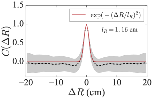
Figure 31: A representative radial correlation function fitted with the function (24) (red line). The points show the measured correlation function $C(\Delta R)$ averaged over $t$ and $Z$ and the shaded region shows the associated standard deviation.

The points show the measured correlation function and the red line the fit (24). The ensemble average is over $t$ and $Z$ and we assume that radial correlations do not change with $t$ and $Z$, i.e., that the system is statistically homogeneous in time and in the poloidal direction. The shaded region in figure 31 indicates the standard deviation calculated over the sum of $t$ and $Z$. We expect that $C(\Delta R)\to 0$ as $\Delta R\to\infty$ (and similarly for subsequent correlation functions in the other directions).

B.2 Poloidal correlation length

The poloidal correlation length is calculated by assuming wave-like fluctuations in the poloidal direction and fitting $C(\Delta R=0,\Delta Z,\lambda(\theta=0),\Delta t=0)$ with an oscillating Gaussian function of the form

$$f_{Z}(\Delta Z)=\cos\quantity(2\pi k_{Z}\Delta Z)\exp\quantity[-{\quantity(\frac{\Delta Z}{l_{Z}})}^{2}],$$ (25)

where $k_{Z}$ is the poloidal wavenumber. Refs. [48, 51] found that with only four poloidal channels, there was insufficient data from the BES diagnostic to fit $l_{Z}$ and $k_{Z}$ independently. As a result, when fitting experimental data (and the data with the synthetic diagnostic applied), the wavenumber is fixed to the value $k_{Z}=2\pi/l_{Z}$. In the direct output of our GS2 simulations, on the other hand, there is a sufficient number of data points in the poloidal direction, to allow us to compare fits both with $k_{Z}$ as a free fitting parameter and fixed in the way described above. Figure 32 shows a representative poloidal correlation function from our simulations along with a fitted function (25), both with fixed $k_{Z}=2\pi/l_{Z}$ [figure 32(a)] and free $k_{Z}$ [figure 32(b)]. The red lines in each plot indicate the fit (25) and the dashed lines indicate the Gaussian envelope $\exp[-{(\Delta Z/l_{Z})}^{2}]$. The ensemble average is over $t$ and $R$. We see that the fit with $k_{Z}$ as a free parameter approximates the correlation function better and predicts a shorter $l_{Z}$. For consistency with previous work, we show the correlation results for both fitting schemes in section 4.4.

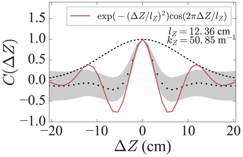
(a)

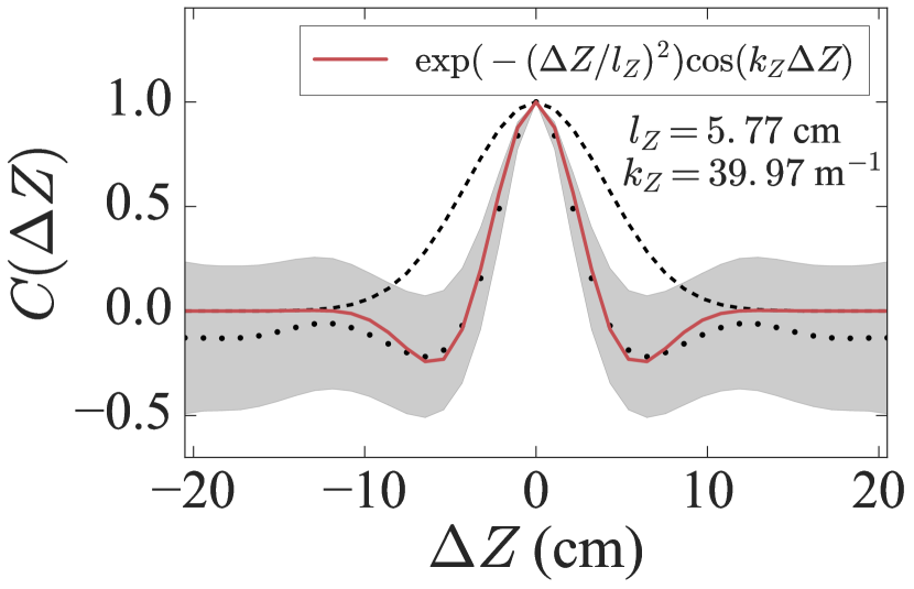
(b)

Figure 32: Representative poloidal correlation function fitted with the function (25) (red line) keeping the poloidal wavenumber $k_{Z}$ 32(a) fixed to $k_{Z}=2\pi/l_{Z}$, 32(b) as an independent fitting parameter. The points in each plot show the correlation function $C(\Delta Z)$ averaged over $t$ and $R$ and the shaded regions show the associated standard deviation. The dashed lines indicate the Gaussian envelope $\exp[-{(\Delta Z/l_{Z})}^{2}]$.

B.3 Correlation time

In the presence of toroidal rotation, turbulent structures are advected in the poloidal direction with an apparent velocity $v_{Z}$ given by [47]

$$v_{Z}=R\omega_{0}\tan\vartheta,$$ (26)

where $\vartheta$ is the magnetic-field pitch-angle (the angle that the field line makes with the midplane on the outboard side of the flux surface). Following [47], we can use this to calculate the correlation time $\tau_{c}$ by tracking turbulent structures as they move poloidally and measuring their temporal decorrelation. This “cross-correlation time delay” technique [44, 47, 49] is as follows. We calculate the correlation function $C_{\Delta Z}(\Delta t)=C(\Delta R=0,\Delta Z,\lambda(\theta=0),\Delta t)$ for several poloidal separations $\Delta Z$, as shown in figure 33. As the structures are advected poloidally, they decorrelate and the peak of the correlation function at a given $\Delta Z$, i.e., the value of $C_{\Delta Z}(\Delta t)$, decreases for increasing $\Delta Z$. The correlation time $\tau_{c}$ is then defined as the characteristic exponential decay time of the peaks of the correlation functions. Namely, we fit $C_{\Delta Z}(\Delta t=\Delta t_{\mathrm{peak}})$ with the function

$$f_{\tau}(\Delta Z)=\exp\quantity[-\quantity|\frac{\Delta t_{\mathrm{peak}}(\Delta Z)}{\tau_{c}}|],$$ (27)

as shown for a representative correlation function in figure 33, where correlation functions $C_{\Delta Z}(\Delta t)$ for different poloidal separations are shown and the red line shows the fit (27).

This method assumes that the temporal decorrelation dominates over any effects due to the finite parallel correlation length, as we will now explain. While turbulent structures are extended along the field lines, they rotate rapidly in the toroidal direction. After accounting for the apparent poloidal motion, a measurement of the correlation time using data from a single poloidal plane will conflate two separate effect: (i) true decorrelation of turbulent structures in time, and (ii) structures of finite parallel length moving past the measurement point. With only data from a single poloidal plane, these two effects are indistinguishable. In order for the true decorrelation of structures in time (which is what we are interested in) to dominate over the movement of structures past the detector, it must be the case that [48]

$$\tau_{c}\ll l_{\parallel}\cos\vartheta/R\omega_{0}.$$ (28)

Since from GS2, unlike from the BES measurements, we can obtain the full 3D turbulence data, we are able to confirm in section 4.4.3 that this condition is indeed satisfied.

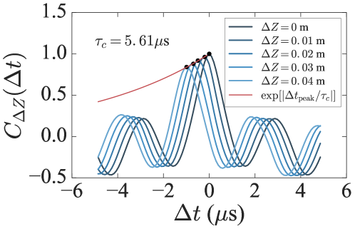
Figure 33: Time correlation functions $C_{\Delta Z}(\Delta t)$ for several poloidal separations $\Delta Z$. The points indicate the maximum value of $C(\Delta t)$ for a given $\Delta Z$, and the red line indicates the function (27) fitted to those points.

B.4 Parallel correlation length

Since GS2 simulations supply the full 3D density-fluctuation field, we are able to study the parallel structure of the turbulence. To do this, we convert the fluctuation field from the GS2 parallel coordinate $\theta$ to a real-space coordinate $\lambda(\theta)$ along the field line, as discussed in Appendix C.3. We then calculate the correlation function $C(\Delta R=0,\Delta Z=0,\Delta\lambda,\Delta t=0)$ and take an average over $(R,Z,t)$. We fit the correlation function with an oscillating Gaussian function of the form

$$f_{\parallel}(\Delta\lambda)=\cos\quantity(2\pi k_{\parallel}\Delta\lambda)\exp\quantity[-{\quantity(\frac{\Delta\lambda}{l_{\parallel}})}^{2}],$$ (29)

where $k_{\parallel}$ is the parallel wavenumber. A representative example of the fitting procedure for the parallel correlation function is shown in figure 34, where the red line indicates the fit (29) and the dashed line shows the Gaussian envelope $\exp[-{(\Delta\lambda/k_{\parallel})}2]$.

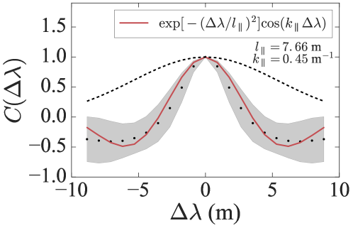
Figure 34: Representative parallel correlation function fitted with the oscillating Gaussian function (29) (red line). The points show the correlation function $C(\Delta\lambda)$ averaged over $(t,R,Z)$ and the shaded region shows the associated standard deviation. The dashed line shows the Gaussian envelope $\exp[-{(\Delta\lambda/k_{\parallel})}^{2}]$.

B.5 Density-fluctuation amplitude

The final simulation prediction we can compare with the experimental results in [51], is the RMS density fluctuation at the outboard midplane ($\theta=0$) averaged over $(t,R,Z)$:

$$\quantity(\frac{\delta n_{i}}{n_{i}})_{\mathrm{rms}}=\left<\frac{\delta n_{i}^{2}(t,R,Z)}{n_{i}^{2}}\right>_{t,R,Z}^{1/2}.$$ (30)

Formally in gyrokinetics, the quantity $\delta n_{i}/n_{i}$ is infinitesimal, and throughout this work, we have written $\delta n_{i}/n_{i}$ to mean $(\rho_{i}/a)\delta n_{i}/n_{i}$, i.e., the physical density-fluctuation field predicted by GS2.

Appendix C Transforming to real space and laboratory frame

GS2 solves the gyrokinetic equation (6) in curvilinear coordinates [93] in a domain known as a “flux tube” (see figure 4), which rotates with the plasma. In order to analyse the real-space structure of turbulence and compare with BES measurements, we need to transform our data from the rotating plasma frame to the laboratory frame and from flux-tube geometry to real-space geometry, i.e., from the GS2 coordinates $(x,y,\theta)$ to $(R,Z,\lambda)$ where $R$ is the major radius, $Z$ is poloidal height above the midplane of the machine, and $\lambda$ is the distance along the field line (not the toroidal direction because correlations are meaningfully long-scale in the direction parallel to the field; see, e.g., [40]).

C.1 Laboratory frame

GS2 simulations are carried out in a frame rotating with the plasma, with toroidal rotation frequency $\omega_{0}$, whereas the BES diagnostic measures turbulence in the laboratory frame. In order to make realistic comparisons with BES measurements, we applied the following transformation to the GS2-calculated distribution function, to transform from the rotating to the laboratory frame [50]:

$$\left(\frac{\delta n_{i}}{n_{i}}\right)_{\mathrm{LAB}}(t,k_{x},k_{y},\theta)=\left(\frac{\delta n_{i}}{n_{i}}\right)_{\mathrm{GS2}}(t,k_{x},k_{y},\theta)e^{-in\omega_{0}t},$$ (31)

where $(\delta n_{i}/n_{i})_{\mathrm{LAB}}$ is the the fluctuating density field calculated by GS2 in the laboratory frame, $(\delta n_{i}/n_{i})_{\mathrm{GS2}}$ is the density field in the rotating plasma frame, and

$$n=k_{y}\rho_{i}\derivative{\psi_{N}}{r}\frac{a}{\rho_{i}}$$ (32)

is the toroidal mode number of a given $k_{y}$ mode, $\psi_{N}$ is the normalised poloidal magnetic flux, $r=D/2a$ is the Miller [56] radial coordinate, $D$ is the diameter of the flux surface, $a$ is half the diameter of the last closed flux surface (LCFS), and $\rho_{i}$ is the ion gyroradius.

C.2 Radial-poloidal domain size

The GS2 flux tube is approximately rectangular at the outboard midplane. Converting from the local GS2 coordinates $(x,y)$ to the radial-poloidal coordinates $(R,Z)$ (the plane of the BES measurement window) is a non-trivial procedure and the reader is referred to [94] for a detailed explanation. Here, we only note that the radial size of the domain is $L_{R}\approx 0.4$ m and the poloidal size of the domain is $L_{Z}\approx 0.81$ m. Figure 35 shows the same plot as in figure 13(a) at $\theta=0$ in terms of the real-space poloidal coordinates $R$ and $Z$. Also indicated in figure 35 are the domains used for the correlation analysis of BES data and raw GS2 data in sections 4.2 and 4.4, respectively.

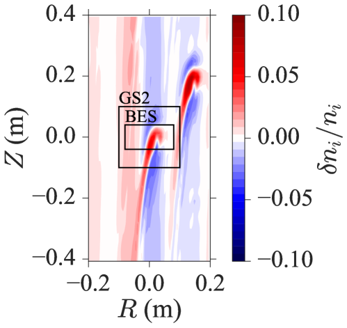
Figure 35: Density-fluctuation field $\delta n_{i}/n_{i}$ as a function $R$ and $Z$ for the same near-marginal case as shown in figure 13(a) for the equilibrium parameters $(\kappa_{T},\gamma_{E})=(4.8,0.16)$. The indicated domains are those used for the correlation analysis of raw GS2 density fluctuations (GS2) and the approximate size of the BES viewing window (BES).

C.3 Parallel coordinate

Finally, we calculate the parallel distance along the magnetic field line at the centre of our flux tube. This procedure is non-trivial for a general geometry because a uniform grid in $\theta$ does not map to a uniform spatial grid along the field line (as it would have done for circular flux surfaces). For our D-shaped geometry, we want to find $\lambda(\theta)$, the distance along the field line parametrised by the poloidal angle $\theta$. The differential arc length of a line element along the field line in terms of $(R,Z,\phi)$ is

$$d\lambda^{2}=dR^{2}+dZ^{2}+{(Rd\phi)}^{2},$$ (33)

where $R=R(\theta)$ and $Z=Z(\theta)$ are the coordinates of the magnetic field line at the centre of the flux tube, and $\phi$ is the toroidal angle. Therefore,

$$\lambda(\theta)=\int_{0}^{\theta}d\theta^{\prime}\sqrt{{\quantity(\derivative{R}{\theta^{\prime}})}^{2}+{\quantity(\derivative{Z}{\theta^{\prime}})}^{2}+{\quantity(R\derivative{\phi}{\theta^{\prime}})}^{2}}.$$ (34)

The quantities $R(\theta)$, $Z(\theta)$, $\derivative*{\phi}{\theta}$ are obtained from the specification of the equilibrium and we then calculate their numerical derivatives with respect to $\theta$ and then the integral (34) to determine $\lambda(\theta)$. With the knowledge of the real-space parallel grid, we can calculate correlation lengths in the parallel direction.

Appendix D Real-space effect of flow shear

Flow shear is implemented in GS2 by allowing the radial wavenumber of each Fourier mode to vary with time [95]:

$$k_{x}^{*}(t)=k_{x}-\gamma_{E}k_{y}t,$$ (35)

where $k_{x}$ would be constant radial Fourier mode in the absence of flow shear. In simplified terms, GS2 shifts the fluctuation fields along the $k_{x}$ dimension as a function of time (see [66] for a complete review of the GS2 flow shear algorithm). This leads to finer radial structure and a displacement of fluctuations in the $y$ direction, as illustrated in figure 36. However, complications arise in this implementation as a result of the fixed $k_{x}$ grid in GS2, which causes jumps in the displacement of fluctuations in the $y$ direction at the radial extremes of the box as we will now explain.

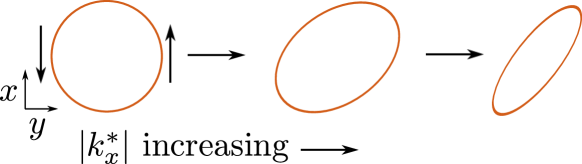
Figure 36: Illustration of the effect of flow shear of turbulent structures. As $k_{x}^{*}$ increases in time there is increased radial structure and displacement in the $y$ direction.

When $k_{x}^{*}$ changes by $\delta k_{x}=\gamma_{E}k_{y}\Delta t$, where $\Delta t$ is a GS2 time step, the value of the GS2 fluctuation fields at $k_{x}$ would ideally be shifted to $k_{x}\pm\delta k_{x}$. However, the $k_{x}$ grid is fixed in GS2 (with a grid separation of $\Delta k_{x}$) and so the fluctuation fields cannot be shifted by less than $\Delta k_{x}$. This issue is resolved in GS2 by keeping track of the difference between the exact shift in $k_{x}$ and the grid spacing $\Delta k_{x}$: when the exact shift is less than $\Delta k_{x}/2$, no shifting takes place but the value is recorded and added to the size of the shift at the next time step. This process is repeated until the shift is greater than or equal to $\Delta k_{x}/2$, at which point all fluctuation fields are shifted by $\Delta k_{x}$. We will now calculate the effect of those shifts.

The distribution function calculated by GS2 is of the form

$$h\propto\exp[i(k_{x}^{*}x+k_{y}y)]=\exp[i(k_{x}x+k_{y}y-\gamma_{E}k_{y}xt)],$$ (36)

where we have substituted for $k_{x}^{*}$ using (35). We can identify the wave frequency $\omega_{h}=\gamma_{E}k_{y}x$ to calculate the group velocity

$${\bf\it v}_{g}=\partialderivative{\omega_{h}}{{\bf\it k}}=-\gamma_{E}x\hat{{\bf\it y}}.$$ (37)

Writing ${\bf\it v}_{g}=\Delta y/\Delta t$, we find the local $x$-dependent displacement of fluctuations in the $y$ direction, for an ideal $k_{x}$ shift of $\delta k_{x}=\gamma_{E}k_{y}\Delta t$,

$$\Delta y=-\frac{\delta k_{x}x}{k_{y}}.$$ (38)

However, $\delta k_{x}$ is forced to match the fixed $k_{x}$ grid with the spacing $\Delta k_{x}=2\pi/L_{x}$, where $L_{x}$ is the size of the box in the $x$ direction. Using $k_{y}=2\pi/\lambda_{y}$, where $\lambda_{y}$ is the wavelength of a given $k_{y}$ mode, we can finally write the displacement due to the flow shear as,

$$\Delta y=\lambda_{y}\frac{x}{L_{x}}.$$ (39)

This means that at the edges of the radial domain, where $x=\pm L_{x}/2$, the displacement in the $y$ direction for every shift in $k_{x}$ due to the flow shear is $\Delta y=\pm\lambda_{y}/2$. The rate of shifting depends on $k_{y}$ according to (35) and so the largest modes (smallest $k_{y}$’s) will be acted on more infrequently than smaller modes (larger $k_{y}$’s). However, the largest modes are then shifted by half the size of their wavelength according to (39). This causes visual separation (or multiplication) of structures at the edges of the GS2 domain in real space in a way that may affect the correlation analyses performed in section 4. For this reason, we have only analysed an area at the centre of the computational domain, shown in figure 35.

We emphasise that the separation of turbulent structures that we have described above is only present in the real-space representation of the GS2 distribution function. Given that GS2 performs calculations (apart from the calculation of nonlinear interactions) in Fourier space, this does not present a problem to the overall calculation. We note that the implementation of flow shear in GS2 is correct in the limit of infinitely small $\Delta k_{x}$ and so it is sufficient to check convergence with $\Delta k_{x}$ to be confident of our results. We performed convergence checks by varying $\Delta k_{x}$ for a fixed maximum $k_{x}$ and confirmed that our results were approximately the same. Ideally, some form of interpolation could be used to smooth out these shifts in $k_{x}$ and a future program of work is planned to implement this in GS2.

Appendix E Correlation analysis without the spike filter

An important step in the analysis of experimental data involves the removal of high-energy radiation (e.g., neutron, gamma ray, or hard X-ray) impinging on the BES detector. This radiation manifests itself as delta-function-like spikes in time, typically only on a single BES channel. These are removed via a numerical “spike filter” [43, 89], which was included in the main analysis (where the synthetic diagnostic was applied; see section 4.3) for consistency with experimental analysis. Here, we show the results of a correlation analysis of GS2 density fluctuations with the synthetic diagnostic applied, but without this spike filter. Figure 37 shows the correlation results for values of $\kappa_{T}$ and $\gamma_{E}$ within the experimental-uncertainty range: the radial correlation length $l^{\mathrm{NS}}_{R}$ [figure 37(a)], the poloidal correlation length $l^{\mathrm{NS}}_{Z}$ [figure 37(b)], the correlation time $\tau^{\mathrm{NS}}_{c}$ [figure 37(c)], the RMS density fluctuation ${(\delta n_{i}/n_{i})}^{\mathrm{NS}}_{\mathrm{rms}}$ [figure 37(d)].

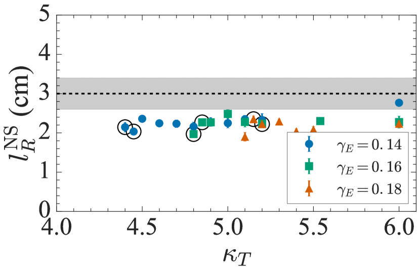
(a)

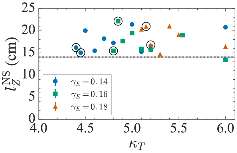
(b)

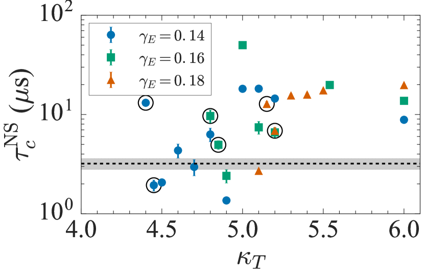
(c)

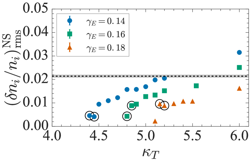
(d)

Figure 37: Correlation-analysis results calculated from the analysis of GS2 fluctuation data (within the region of experimental uncertainty) after applying the synthetic diagnostic, but without the spike filter normally applied to experimental data (see figure 24): 37(a) radial correlation length $l_{R}^{\mathrm{NS}}$ (section B.1), 37(b) poloidal correlation length $l_{Z}^{\mathrm{NS}}$ (section B.2), 37(c) correlation time $\tau_{c}^{\mathrm{NS}}$ (section B.3), and 37(d) RMS fluctuation amplitude $\quantity(\delta n_{i}/n_{i})^{\,\mathrm{NS}}_{\mathrm{rms}}$ (section B.5). The simulations that matched the experimental heat flux are circled. The quantities plotted here are discussed in appendix B.

Comparing these results to the results in section 4.3 with the spike filter, we see that it is mainly the poloidal correlation length that is affected: $l^{\mathrm{NS}}_{Z}$ is several centimetres lower with the spike filter compared to cases without it. We found that in some cases, fast-moving structures in the poloidal direction (especially the long-lived structures found in our near-marginal simulations; see section 3.3.1) were removed by the spike filter and, therefore, did not affect the poloidal correlation function thus copmputed, resulting in a drop in $l^{\mathrm{NS}}_{Z}$. In particular, figure 37(b) shows that $l^{\mathrm{NS}}_{Z}$ increased significantly in near-marginal simulations compared to its values obtained with the spike filter. This observation of the vulnerability of coherent structures predicted by our simulations to the spike filter should inform future attempts to observe these structures experimentally.

References

- [1] K. Krushelnick and S. Cowley. Reduced turbulence and new opportunities for fusion. Science, 309:1502, 2005.
- [2] B. Coppi, M. N. Rosenbluth, and R. Z. Sagdeev. Instabilities due to temperature gradients in complex magnetic field configurations. Phys. Fluids, 10(3):582, 1967.
- [3] S. C. Cowley, R. M. Kulsrud, and R. Sudan. Considerations of ion-temperature-gradient-driven turbulence. Phys. Fluids B, 3(10):2767, 1991.
- [4] D. J. Applegate, C. M. Roach, J. W. Connor, S. C. Cowley, W. Dorland, R. J. Hastie, and N. Joiner. Micro-tearing modes in the mega ampere spherical tokamak. Plasma Phys. Control. Fusion, 49(8):1113, 2007.
- [5] T. Dannert and F. Jenko. Gyrokinetic simulation of collisionless trapped-electron mode turbulence. Phys. Plasmas, 12(7):1, 2005.
- [6] W. Dorland, F. Jenko, M. Kotschenreuther, and B. N. Rogers. Electron temperature gradient turbulence. Phys. Rev. Lett., 85(26):5579, 2000.
- [7] F. Jenko, W. Dorland, M. Kotschenreuther, and B. N. Rogers. Electron temperature gradient driven turbulence. Phys. Plasmas, 7(5):1904, 2000.
- [8] P. Mantica, D. Strintzi, T. Tala, C. Giroud, T. Johnson, H. Leggate, E. Lerche, T. Loarer, A. G. Peeters, A. Salmi, S. Sharapov, D. Van Eester, P. C. De Vries, L. Zabeo, and K.-D. Zastrow. Experimental study of the ion critical-gradient length and stiffness level and the impact of rotation in the JET Tokamak. Phys. Rev. Lett., 102(17):1, 2009.
- [9] P. Mantica, C. Angioni, C. Challis, G. Colyer, L. Frassinetti, N. Hawkes, T. Johnson, M. Tsalas, P. C. DeVries, J. Weiland, B. Baiocchi, M. N. A. Beurskens, A. C. A. Figueiredo, C. Giroud, J. Hobirk, E. Joffrin, E. Lerche, V. Naulin, A. G. Peeters, A. Salmi, C. Sozzi, D. Strintzi, G. Staebler, T. Tala, D. Van Eester, and T. Versloot. A key to improved ion core confinement in the JET tokamak: ion stiffness mitigation due to combined plasma rotation and low magnetic shear. Phys. Rev. Lett., 107(13):135004, 2011.
- [10] J. Citrin, F. Jenko, P. Mantica, D. Told, C. Bourdelle, R. Dumont, J. Garcia, J. W. Haverkort, G. M. D. Hogeweij, T. Johnson, and M. J. Pueschel. Ion temperature profile stiffness: non-linear gyrokinetic simulations and comparison with experiment. Nucl. Fusion, 54:023008, 2014.
- [11] J. C. Hillesheim, J. C. DeBoo, W. A. Peebles, T. A. Carter, G. Wang, T. L. Rhodes, L. Schmitz, G. R. McKee, Z. Yan, G. M. Staebler, K. H. Burrell, E. J. Doyle, C. Holland, C. C. Petty, S. P. Smith, A. E. White, and L. Zeng. Observation of a Critical Gradient Threshold for Electron Temperature Fluctuations in the DIII-D Tokamak. Phys. Rev. Lett., 110(4):045003, 2013.
- [12] R. J. Akers, J. W. Ahn, G. Y. Antar, L. C. Appel, D. Applegate, C. Brickley, C. Bunting, P. G. Carolan, C. D. Challis, N. J. Conway, G. F. Counsell, R. O. Dendy, B. Dudson, A. R. Field, A. Kirk, B. Lloyd, H. F. Meyer, A. W. Morris, A. Patel, C. M. Roach, V. Rohzansky, A. Sykes, D. Taylor, M. R. Tournianski, M. Valovic, H. R. Wilson, K. B. Axon, R. J. Buttery, D. Ciric, G. Cunningham, J. Dowling, M. R. Dunstan, S. J. Gee, M. P. Gryaznevich, P. Helander, D. L. Keeling, P. J. Knight, F. Lott, M. J. Loughlin, S. J. Manhood, R. Martin, G. J. McArdle, M. N. Price, K. Stammers, J. Storrs, M. J. Walsh, and the MAST and NBI team. Transport and confinement in the Mega Ampère Spherical Tokamak (MAST) plasma. Plasma Phys. Control. Fusion, 45(12A):A175, 2003.
- [13] C. M. Roach, D. J. Applegate, J. W. Connor, S. C. Cowley, W. D. Dorland, R J Hastie, N Joiner, S Saarelma, A. A. Schekochihin, R. J. Akers, C Brickley, A. R. Field, M. Valovic, and the Mast Team. Microstability physics as illuminated in the spherical tokamak. Plasma Phys. Control. Fusion, 47(12B):B323, 2005.
- [14] N. Joiner, D. Applegate, S. C. Cowley, W. Dorland, and C. M. Roach. Electron temperature gradient driven transport in a MAST H-mode plasma. Plasma Phys. Control. Fusion, 48(48):685, 2006.
- [15] D. J. Applegate, C. M. Roach, S. C. Cowley, W. D. Dorland, N. Joiner, R. J. Akers, N. J. Conway, A. R. Field, A. Patel, M. Valovic, and M. J. Walsh. Microstability in a “MAST-like” high confinement mode spherical tokamak equilibrium. Phys. Plasmas, 11(11):5085, 2004.
- [16] D. Dickinson, C. M. Roach, S. Saarelma, R. Scannell, A. Kirk, and H. R. Wilson. Kinetic instabilities that limit in the edge of a tokamak plasma: A picture of an H-mode pedestal. Phys. Rev. Lett., 108(13):1, 2012.
- [17] J. C. Hillesheim, D. Dickinson, C. M. Roach, S. Saarelma, R. Scannell, A. Kirk, N. A. Crocker, W. A. Peebles, and H. Meyer. Intermediate-k density and magnetic field fluctuations during inter-ELM pedestal evolution in MAST. Plasma Phys. Control. Fusion, 58(1):014020, 2016.
- [18] F. M. Levinton, H. Yuh, M. G. Bell, R. E. Bell, L. Delgado-Aparicio, M. Finkenthal, E. D. Fredrickson, D. A. Gates, S. M. Kaye, B. P. LeBlanc, R. Maingi, J. E. Menard, D. Mikkelsen, D. Mueller, R. Raman, G. Rewoldt, S. A. Sabbagh, D. Stutman, K. Tritz, and W. Wang. Transport with reversed shear in the National Spherical Torus Experiment. Phys. Plasmas, 14(5), 2007.
- [19] K. L. Wong, S. Kaye, D. R. Mikkelsen, J. A. Krommes, K. Hill, R. Bell, and B. Leblanc. Microtearing instabilities and electron transport in the NSTX spherical tokamak. Phys. Rev. Lett., 99(13):1, 2007.
- [20] K. L. Wong, S. Kaye, D. R. Mikkelsen, J. A. Krommes, K. Hill, R. Bell, and B. LeBlanc. A quantitative account of electron energy transport in a National Spherical Tokamak Experiment plasma. Phys. Plasmas, 15(5):056108, 2008.
- [21] W. Guttenfelder, J. Candy, S. M. Kaye, W. M. Nevins, E. Wang, R. E. Bell, G. W. Hammett, B. P. Leblanc, D. R. Mikkelsen, and H. Yuh. Electromagnetic transport from microtearing mode turbulence. Phys. Rev. Lett., 106(15):1, 2011.
- [22] W. Guttenfelder, J. Candy, S. M. Kaye, W. M. Nevins, E. Wang, J. Zhang, R. E. Bell, N. A. Crocker, G. W. Hammett, B. P. Leblanc, D. R. Mikkelsen, Y. Ren, and H. Yuh. Simulation of microtearing turbulence in national spherical torus experiment. Phys. Plasmas, 19(5):1, 2012.
- [23] W. Guttenfelder, J. L. Peterson, J. Candy, S. M. Kaye, Y. Ren, R. E. Bell, G. W. Hammett, B. P. LeBlanc, D. R. Mikkelsen, W. M. Nevins, and H. Yuh. Progress in simulating turbulent electron thermal transport in NSTX. Nucl. Fusion, 53(9):093022, 2013.
- [24] K. H. Burrell. Effects of ExB velocity shear and magnetic shear on turbulence and transport in magnetic confinement devices. Phys. Plasmas, 4(5):1499, 1997.
- [25] A. R. Field, C. Michael, R. J. Akers, J. Candy, G. Colyer, W. Guttenfelder, Y.-c. Ghim, C. M. Roach, and S. Saarelma. Plasma rotation and transport in MAST spherical tokamak. Nucl. Fusion, 51(6):063006, 2011.
- [26] Y.-c. Ghim, A. R. Field, A. A. Schekochihin, E. G. Highcock, C. Michael, and the MAST Team. Local dependence of ion temperature gradient on magnetic configuration, rotational shear and turbulent heat flux in MAST. Nucl. Fusion, 54(4):6, 2014.
- [27] T. S. Hahm and K. H. Burrell. Flow shear induced fluctuation suppression in finite aspect ratio shaped tokamak plasma. Phys. Plasmas, 2(5):1648, 1995.
- [28] C. M. Roach, I. G. Abel, R. J. Akers, W. Arter, M. Barnes, Y. Camenen, F. J. Casson, G. Colyer, J. W. Connor, S. C. Cowley, D. Dickinson, W. D. Dorland, A. R. Field, W. Guttenfelder, G. W. Hammett, R. Hastie, E. G. Highcock, N. F. Loureiro, A. G. Peeters, M. Reshko, S. Saarelma, A. A. Schekochihin, M. Valovic, and H. R. Wilson. Gyrokinetic simulations of spherical tokamaks. Plasma Phys. Control. Fusion, 51(12):124020, 2009.
- [29] S. M. Kaye, R. E. Bell, D. Gates, B. P. LeBlanc, F. M. Levinton, J. E. Menard, D. Mueller, G. Rewoldt, S. A. Sabbagh, W. Wang, and H. Yuh. Scaling of Electron and Ion Transport in the High-Power Spherical Torus NSTX. Phys. Rev. Lett., 98(17):175002, 2007.
- [30] S. M. Kaye, S. Gerhardt, W. Guttenfelder, R. Maingi, R. E. Bell, A. Diallo, B. P. LeBlanc, and M. Podesta. The dependence of H-mode energy confinement and transport on collisionality in NSTX. Nucl. Fusion, 53(6):063005, 2013.
- [31] P. J. Catto. Parallel velocity shear instabilities in an inhomogeneous plasma with a sheared magnetic field. Phys. Fluids, 16(10):1719, 1973.
- [32] M. Barnes, F. I. Parra, E. G. Highcock, A. A. Schekochihin, S. C. Cowley, and C. M. Roach. Turbulent transport in tokamak plasmas with rotational shear. Phys. Rev. Lett., 106(17):175004, 2011.
- [33] S. L. Newton, S. C. Cowley, and N. F. Loureiro. Understanding the effect of sheared flow on microinstabilities. Plasma Phys. Control. Fusion, 52(12):125001, 2010.
- [34] E. G. Highcock, M. Barnes, F. I. Parra, A. A. Schekochihin, C. M. Roach, and S. C. Cowley. Transport bifurcation induced by sheared toroidal flow in tokamak plasmas. Phys. Plasmas, 18(10):102304, 2011.
- [35] A. A. Schekochihin, E. G. Highcock, and S. C. Cowley. Subcritical fluctuations and suppression of turbulence in differentially rotating gyrokinetic plasmas. Plasma Phys. Control. Fusion, 54(5):055011, 2012.
- [36] M. Landreman, G. G. Plunk, and W. D. Dorland. Generalized universal instability: transient linear amplification and subcritical turbulence. J. Plasma Phys., 81(05):905810501, 2015.
- [37] F. van Wyk, E. G. Highcock, A. A. Schekochihin, C. M. Roach, A. R. Field, and W. Dorland. Transition to subcritical turbulence in a tokamak plasma. J. Plasma Phys., 82(6):905820609, 2016.
- [38] E. A. Frieman and L. Chen. Nonlinear gyrokinetic equations for low-frequency electromagnetic waves in general plasma equilibria. Phys. Fluids, 25(3):502, 1982.
- [39] H. Sugama and W. Horton. Nonlinear electromagnetic gyrokinetic equation for plasmas with large mean flows. Phys. Plasmas, 5(7):2560, 1998.
- [40] I. G. Abel, G. G. Plunk, E. Wang, M. Barnes, S. C. Cowley, W. D. Dorland, and A. A. Schekochihin. Multiscale gyrokinetics for rotating tokamak plasmas: fluctuations, transport and energy flows. Rep. Prog. Phys., 76(11):105, 2013.
- [41] M. Kotschenreuther, G. Rewoldt, and W. M. Tang. Comparison of initial value and eigenvalue codes for kinetic toroidal plasma instabilities. Comput. Phys. Commun., 88(2):128, 1995.
- [42] A. R. Field, D. Dunai, N. J. Conway, S. Zoletnik, and J. Sárközi. Beam emission spectroscopy for density turbulence measurements on the MAST spherical tokamak. Rev. Sci. Instrum., 80(7):073503, 2009.
- [43] A. R. Field, D. Dunai, R. Gaffka, Y.-c. Ghim, I. Kiss, B. Mészáros, T. Krizsanóczi, S. Shibaev, and S. Zoletnik. Beam emission spectroscopy turbulence imaging system for the MAST spherical tokamak. Rev. Sci. Instrum., 83(1):013508, 2012.
- [44] R. D. Durst, R. J. Fonck, G. Cosby, H. Evensen, and S. F. Paul. Density fluctuation measurements via beam emission spectroscopy. Rev. Sci. Instrum., 63(10):4907, 1992.
- [45] G. R. McKee, C. Fenzi, R. J. Fonck, and M. Jakubowski. Turbulence imaging and applications using beam emission spectroscopy on DIII-D (invited). Rev. Sci. Instrum., 74(3 II):2014, 2003.
- [46] M. W. Shafer, R. J. Fonck, G. R. McKee, C. Holland, A. E. White, and D. J. Schlossberg. 2D properties of core turbulence on DIII-D and comparison to gyrokinetic simulations. Phys. Plasmas, 19(3):032504, 2012.
- [47] Y.-c. Ghim, A. R. Field, D. Dunai, S. Zoletnik, L. Bardóczi, and A. A. Schekochihin. Measurement and physical interpretation of the mean motion of turbulent density patterns detected by the beam emission spectroscopy system on the Mega Amp Spherical Tokamak. Plasma Phys. Control. Fusion, 54(9):095012, 2012.
- [48] Y.-c. Ghim, A. A. Schekochihin, A. R. Field, I. G. Abel, M. Barnes, G. Colyer, S. C. Cowley, F. I. Parra, D. Dunai, and S. Zoletnik. Experimental signatures of critically balanced turbulence in MAST. Phys. Rev. Lett., 110(14):145002, 2013.
- [49] M. F. J. Fox, A. R. Field, F van Wyk, Y.-c. Ghim, and A. A. Schekochihin. Experimental determination of the correlation properties of plasma turbulence using 2D BES systems. Plasma Phys. Control. Fusion, 59(4):044008, 2017.
- [50] C. Holland, A. E. White, G. R. McKee, M. W. Shafer, J. Candy, R. E. Waltz, L. Schmitz, and G. R. Tynan. Implementation and application of two synthetic diagnostics for validating simulations of core tokamak turbulence. Phys. Plasmas, 16(5):052301, 2009.
- [51] A. R. Field, D. Dunai, Y.-c. Ghim, P. Hill, B. F. McMillan, C. M. Roach, S. Saarelma, A. A. Schekochihin, and S. Zoletnik. Comparison of BES measurements of ion-scale turbulence with direct gyro-kinetic simulations of MAST L-mode plasmas. Plasma Phys. Control. Fusion, 56(2):025012, 2014.
- [52] G. R. McKee, R. Ashley, R. D. Durst, R. J. Fonck, M.W. Jakubowski, K. Tritz, K. H. Burrell, C. Greenfield, and J. Robinson. The beam emission spectroscopy diagnostic on the DIII-D tokamak. Rev. Sci. Instrum., 70(1):913, 1999.
- [53] C. Holland, L. Schmitz, T. L. Rhodes, W. A. Peebles, J. C. Hillesheim, G. Wang, L. Zeng, E. J. Doyle, S. P. Smith, R. Prater, K. H. Burrell, J. Candy, R. E. Waltz, J. E. Kinsey, G. M. Staebler, J. C. DeBoo, C. C. Petty, G. R. McKee, Z. Yan, and A. E. White. Advances in validating gyrokinetic turbulence models against L- and H-mode plasmas. Phys. Plasmas, 18(5):056113, 2011.
- [54] T. L. Rhodes, C. Holland, S. P. Smith, A. E. White, K. H. Burrell, J. Candy, J. C. DeBoo, E. J. Doyle, J. C. Hillesheim, J. E. Kinsey, G. R. McKee, D. Mikkelsen, W. A. Peebles, C. C. Petty, R. Prater, S. Parker, Y. Chen, L. Schmitz, G. M. Staebler, R. E. Waltz, G. Wang, Z. Yan, and L. Zeng. L-mode validation studies of gyrokinetic turbulence simulations via multiscale and multifield turbulence measurements on the DIII-D tokamak. Nucl. Fusion, 51(6):63022, 2011.
- [55] T. Görler, A. E. White, D. Told, F. Jenko, C. Holland, and T. L. Rhodes. A flux-matched gyrokinetic analysis of DIII-D L-mode turbulence. Phys. Plasmas, 21(12):0, 2014.
- [56] R. L. Miller, M. S. Chu, J. M. Greene, Y. R. Lin-Liu, and R. E. Waltz. Noncircular, finite aspect ratio, local equilibrium model. Phys. Plasmas, 5(4):973, 1998.
- [57] N. J. Conway, P. G. Carolan, J. McCone, M. J. Walsh, and M. Wisse. High-throughput charge exchange recombination spectroscopy system on MAST. Rev. Sci. Instrum., 77(10):10F131, 2006.
- [58] R. Scannell, M. J. Walsh, M. R. Dunstan, J. Figueiredo, G. Naylor, T. O’Gorman, S. Shibaev, K. J. Gibson, and H. Wilson. A 130 point Nd:YAG Thomson scattering diagnostic on MAST. Rev. Sci. Instrum., 81(10):10D520, 2010.
- [59] L. L. Lao, H. St. John, R. D. Stambaugh, A. G. Kellman, and W. Pfeiffer. Reconstruction of current profile parameters and plasma shapes in tokamaks. Nucl. Fusion, 25(11):1611, 1985.
- [60] R. J. Hawryluk. An emperical approach to tokamak transport. In B. Coppi, editor, Phys. Plasmas Close to Thermonucl. Cond., volume 1, page 19. Elsevier, 1981.
- [61] I. G. Abel, M. Barnes, S. C. Cowley, W. D. Dorland, and A. A. Schekochihin. Linearized model Fokker–Planck collision operators for gyrokinetic simulations. I. Theory. Phys. Plasmas, 15(12):122509, 2008.
- [62] M. Barnes, I. G. Abel, W. Dorland, D. R. Ernst, G. W. Hammett, P. Ricci, B. N. Rogers, A. A. Schekochihin, and T. Tatsuno. Linearized model Fokker–Planck collision operators for gyrokinetic simulations. II. Numerical implementation and tests. Phys. Plasmas, 16(7):072107, 2009.
- [63] B. F. McMillan, X. Lapillonne, S. Brunner, L. Villard, S. Jolliet, A. Bottino, T. Görler, and F. Jenko. System Size Effects on Gyrokinetic Turbulence. Phys. Rev. Lett., 105(15):155001, 2010.
- [64] S. Saarelma, P. Hill, A. Bottino, G. Colyer, A. R. Field, B. F. McMillan, A. G. Peeters, and C. M. Roach. Global gyrokinetic turbulence simulations of MAST plasmas. Plasma Phys. Control. Fusion, 54(8):085012, 2012.
- [65] F. I. Parra and M. Barnes. Equivalence of two different approaches to global f gyrokinetic simulations. Plasma Phys. Control. Fusion, 57(5):054003, 2015.
- [66] E. G. Highcock. The zero turbulence manifold in fusion plasmas. 2012. arXiv:1207.4419.
- [67] A. M. Dimits, G. Bateman, M. A. Beer, B. I. Cohen, W. D. Dorland, G. W. Hammett, C. Kim, J. E. Kinsey, M. Kotschenreuther, A. H. Kritz, L. L. Lao, J. Mandrekas, W. M. Nevins, S. E. Parker, A. J. Redd, D. E. Shumaker, R. Sydora, and J. Weiland. Comparisons and physics basis of tokamak transport models and turbulence simulations. Phys. Plasmas, 7(3):969, 2000.
- [68] G. J. Colyer, A. A. Schekochihin, F. I. Parra, C. M. Roach, M. A. Barnes, Y.-c. Ghim, and W. Dorland. Collisionality scaling of the electron heat flux in ETG turbulence. Plasma Phys. Control. Fusion, 59(5):055002, 2017.
- [69] N.T. Howard, C. Holland, A.E. White, M. Greenwald, and J. Candy. Multi-scale gyrokinetic simulation of tokamak plasmas: enhanced heat loss due to cross-scale coupling of plasma turbulence. Nucl. Fusion, 56(1):014004, 2016.
- [70] N. T. Howard, C. Holland, A. E. White, M. Greenwald, J. Candy, and A. J. Creely. Multi-scale gyrokinetic simulations: Comparison with experiment and implications for predicting turbulence and transport. Phys. Plasmas, 23(5):056109, 2016.
- [71] E. G. Highcock, M. Barnes, A. A. Schekochihin, F. I. Parra, C. M. Roach, and S. C. Cowley. Transport bifurcation in a rotating tokamak plasma. Phys. Rev. Lett., 105(21):215003, 2010.
- [72] L. N. Trefethen, A. E. Trefethen, S. C. Reddy, and T. A. Driscoll. Hydrodynamic stability without eigenvalues. Science, 261(5121):578, 1993.
- [73] E. G. Highcock, A. A. Schekochihin, S. C. Cowley, M. Barnes, F. I. Parra, C. M. Roach, and W. Dorland. Zero-turbulence manifold in a toroidal plasma. Phys. Rev. Lett., 109(26):265001, 2012.
- [74] H. Faisst and B. Eckhardt. Sensitive dependence on initial conditions in transition to turbulence in pipe flow. J. Fluid Mech., 504:343, 2004.
- [75] J. Peixinho and T. Mullin. Decay of turbulence in pipe flow. Phys. Rev. Lett., 96(9):094501, 2006.
- [76] B. Hof, J. Westerweel, T. M. Schneider, and B. Eckhardt. Finite lifetime of turbulence in shear flows. Nature, 443(7107):59, 2006.
- [77] K. Avila, D. Moxey, A. de Lozar, M. Avila, D. Barkley, and B. Hof. The onset of turbulence in pipe flow. Science, 333(6039):192, 2011.
- [78] M. Avila, A. P. Willis, and B. Hof. On the transient nature of localized pipe flow turbulence. J. Fluid Mech., 646:127, 2010.
- [79] E. L. Rempel, G. Lesur, and M. R. E. Proctor. Supertransient magnetohydrodynamic turbulence in keplerian shear flows. Phys. Rev. Lett., 105(4):044501, 2010.
- [80] R. E. Waltz. Three-dimensional global numerical simulation of ion temperature gradient mode turbulence. Phys. Fluids, 31(7):1962, 1988.
- [81] A. M. Dimits, T. J. Williams, J. A. Byers, and B. I. Cohen. Scalings of ion-temperature-gradient-driven anomalous transport in tokamaks. Phys. Rev. Lett., 77:71, 1996.
- [82] B. N. Rogers, W. Dorland, and M. Kotschenreuther. Generation and stability of zonal flows in ion-temperature-gradient mode turbulence. Phys. Rev. Lett., 85(25):5336, 2000.
- [83] S. van der Walt, J. L. Schönberger, J. Nunez-Iglesias, F. Boulogne, J. D. Warner, N. Yager, E. Gouillart, T. Yu, and the scikit-image contributors. scikit-image: image processing in Python. PeerJ, 2:e453, 2014.
- [84] C. Fiorio and J. Gustedt. Two linear time Union-Find strategies for image processing. Theor. Comput. Sci., 154(2):165, 1996.
- [85] R. E. Waltz, G. D. Kerbel, and J. Milovich. Toroidal gyro-Landau fluid model turbulence simulations in a nonlinear ballooning mode representation with radial modes. Phys. Plasmas, 1(7):2229, 1994.
- [86] Z. Lin, T. S. Hahm, W. W. Lee, W. M. Tang, and R. B. White. Turbulent transport reduction by zonal flows: massively parallel simulations. Science, 281(5384):1835, 1998.
- [87] P. H. Diamond, S.-I. Itoh, K. Itoh, and T. S. Hahm. Zonal flows in plasma—a review. Plasma Phys. Control. Fusion, 47(5):R35, 2005.
- [88] M. Barnes, F. I. Parra, and A. A. Schekochihin. Critically balanced ion temperature gradient turbulence in fusion plasmas. Phys. Rev. Lett., 107(11):115003, 2011.
- [89] M. F. J. Fox, F. van Wyk, A. R. Field, Y-c Ghim, F. I. Parra, and A. A. Schekochihin. Symmetry breaking in MAST plasma turbulence due to toroidal flow shear. Plasma Phys. Control. Fusion, 59(3):034002, 2017.
- [90] Ch. P. Ritz, H. Lin, T. L. Rhodes, and A. J. Wootton. Evidence for confinement improvement by velocity-shear suppression of edge turbulence. Phys. Rev. Lett., 65(20):2543, 1990.
- [91] D. Barkley, B. Song, V. Mukund, G. Lemoult, M. Avila, and B. Hof. The rise of fully turbulent flow. Nature, 526(7574):550, 2015.
- [92] J. C. Hillesheim, N. A. Crocker, W. A. Peebles, H. Meyer, A. Meakins, A. R. Field, D. Dunai, M. Carr, and N. Hawkes. Doppler backscattering for spherical tokamaks and measurement of high-k density fluctuation wavenumber spectrum in MAST. Nucl. Fusion, 55(7):073024, 2015.
- [93] M. A. Beer, S. C. Cowley, and G. W. Hammett. Field-aligned coordinates for nonlinear simulations of tokamak turbulence. Phys. Plasmas, 2(7):2687, 1995.
- [94] F. van Wyk. Subcritical turbulence in the mega ampere spherical tokamak. 2017. arXiv:1703.03397.
- [95] G. W Hammett, W. Dorland, N. F. Loureiro, and T. Tatsuno. Implementation of large scale ExB shear flow in the GS2 gyrokinetic turbulence code. In APS Meeting Abstracts, 2006. Presented at the 48th Annual Meeting of the Division of Plasma Physics, Abstract No. VP1.00136.