Line-soliton and rational solutions to (2+1)-dimensional Boussinesq equation by Dbar-problem
Abstract
We present a generalized (2+1)-dimensional Boussinesq equation, including two cases which are called the plus Boussinesq equation
and the minus one. To investigate these equations, we
apply the approach to a coupled (2+1)-dimensional nonlinear equation, which reduces to the Boussinesq equation.
For the plus equation, we give the line-solitons and rational solutions, for the minus one, we give some freak solutions.
Keywords: Boussinesq equation, Dbar-problem, line-soliton,rational solution
1 Introduction
The method based on the (Dbar)-problem [1, 2, 3, 4] is a powerful tool to investigate the integrability of nonlinear PDEs , especially higher dimensional equations, and to find their explicit solutions, including solitons and rational solutions. The departure from analyticity of a complex function can be measured by the Dbr derivative, a special case of this departure is the jump condition for sectionally analytic function in the Riemann-Hilbert problem. However, if the associated eigenfunctions is analytic nowhere, the Riemann-Hilbert approach fails, but the Dbar approach still works [5].
We consider a (2+1)-dimensional coupled nonlinear equation [6]
| (1) | |||
where . The method we used in this paper is based on the Dbar-problem in complex plane
| (2) |
with canonical normalization at . Here the domain of the integration is the complex plane, and will be omitted in the paper.
System (1) after elimination of reduces to a generalized (2+1)-dimensional Boussinesq equation
| (3) |
which can be reduces to the classical Boussinesq equation (see, e.g. [7, 8, 9, 10, 11]). The Boussinesq equation is integrable by the inverse problem method (see, [12, 13, 14, 10, 15]), the Lax pair for this equation was constructed in [16]. We now consider the following form of solution [17, 18]
| (4) |
For , (4) is a small amplitude solution, which make the nonlinear term of (3) negligible. In this case, the time frequency of (4) is complex, but we get the exponential growth at a rate of about . while, for , the amplitude of solution (4) is , which is ill-posed for . In the following, we call the Boussinesq equation (3) with the ”plus” type, and be ”minus” type.
We note that Bogdanov and Zakharov investigated the continuous spectrum and soliton solutions for the two type Boussinesq equations (named ”plus” and ”minus” Boussinesq equations) by using the Dbar-dressing method [17]. In that paper, the Boussinesq equation is a dimensional reduction in the framework of the KP hierarchy. So the associated covariant derivative is related to that of KP equation. In this paper, the generalized (2+1)-dimensional Boussinesq equation (3) is derived from different covariant derivative.
Although the two type equations have different properties, we present a useful method to discuss them at same time. For the plus Boussinesq equation, we obtain line-soliton and rational solutions by choosing special degenerate kernel of the Dbar problem. We note that the line-soliton solutions are complexiton solutions [19, 20, 21, 22], which show some periodic motions. In addition, the rational solution can not be reduced to the lump solution for the plus Boussinesq equation. For minus equation, we give some explicit solutions which show some strange appearance. Here we call them freak solutions. It is remarked that the rational solutions for the plus Boussinesq equation also show some strange properties.
In [6], the author only studied the case of of system (1) by Darboux transformation and gave some periodic solutions. In the last part of this paper, we also extend the Darboux transformation to both cases of the Boussinesq equation, and obtain some new rational solution and freak solution, respectively. The present equation is different from the known (2+1)-dimensional Boussinesq equations studied in [23, 24, 25].
The paper is organized as follows. In Section 2, the Dbar dressing method is presented to derive the Lax pair of a coupled (2+1)-dimensional nonlinear equation system, which can be reduced to the generalized (2+1)-dimensional Boussinesq equation. In section 3, the explicit solutions, including line-solitons and rational solutions, are given by virtue of different choice of the kernel of the Dbar problem. We give some discussions in the last section, and present some novel solutions by extending the method used in [6].
2 Dbar dressing Method
Since the time frequency of (4) is complex, we consider the wave number is , in stead of , for convenience. So, we introduce a set of operators as
| (5) |
and the general kernel of the Dbar-problem is
| (6) |
Here is an arbitrary function and
| (7) |
Suppose that the analytic function has the following expansion
| (8) |
It is readily verified that the following two expressions have no singularity at
| (9) | |||
where
| (10) |
Thus, according to the Liouville’s theorem, we have two linear equations
| (11) |
and
| (12) |
It is noted that the second linear equation takes another form
| (13) |
3 Solutions
It is noted that the Dbar-problem (2) with the canonical normalization is equivalent to a integral equation
| (16) |
In the case of the degenerate kernel
| (17) |
the linear integral equation (16) is reduced to the linear algebraic system. Suppose that the solution of problem (16) has the asymptotic behaviors (8), then
| (18) |
where
| (19) |
and
| (20) |
3.1 Line Solitons
Existing the soliton solution is an important property for the integrable system. To derive the line solitons, we consider functions and in the kernel (17) as
| (21) |
where and are constants. Here the function is defined by (7). In this case, from (19) and (20), we have
| (22) |
Now, the representations in (18) can be rewritten as the following form
| (23) |
the block matrix and are defined by
| (24) |
where the row vectors and are defined as
| (25) |
Substitution (23) into (10), we have the explicit solution of the system (1). We note that the representation will give the explicit solution of the generalized (2+1)-dimensional Boussinesq equation (3). In the following, we will not to put stress on it.
Particularly, for , we have
| (26) |
where . Furthermore, if let , we obtain one line-soliton solution
| (27) | ||||
where
| (28) | ||||
Here, for ,
| (29) | ||||
and for ,
| (30) | ||||
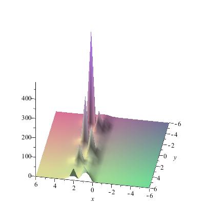
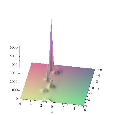
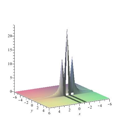
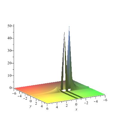
For the case of , that is solution (27) and (28) with (29), the frequency is two times the wave number in direction. In this case, the one line-soliton shows a periodic motion (see Fig. 1), and the periodicity will be more clear in the case and , which are removable singularities (see Fig. 2).
While, for the case of and (30), the phase will play an important role in the wave motion, which give a freak wave (see Fig. 3).
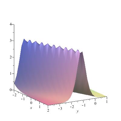
Abs(u)(t=0),
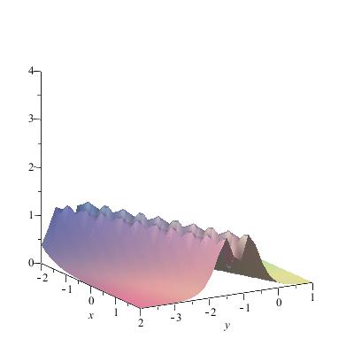
Abs(v)(t=0),
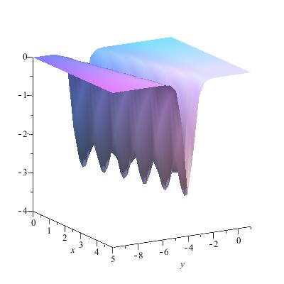
u(t=),
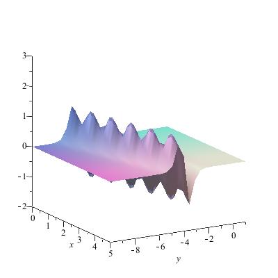
v(t=),
Abs(u)(t=),
Abs(v)(t=),
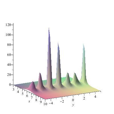
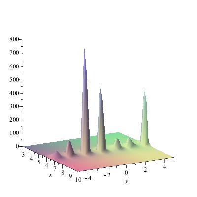
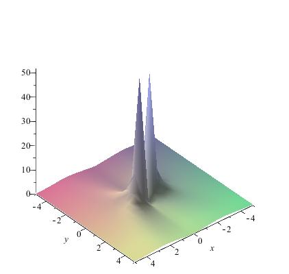
For and , the figure of the two line-soliton (10),(23) and (24) with , is shown in Fig. 4. In Fig. 5, it shows the two-freak wave for and .
Abs(u)(t=0),
Abs(v)(t=0),
Abs(u)(t=0),
Abs(v)(t=0),
3.2 Rational solutions
To obtain the rational solutions of the equations in (1), we choose the kernel as
| (31) |
where and are smooth functions. Substituting into (16), we have a representation of
| (32) |
where . For convenience, we choose and , then (32) reduces to
| (33) |
We note that can be obtained from (16) and (31) by letting , that is
If one introduce the following matrices
| (34) | |||
then
From (32), one find that has the following asymptotic behavior
where
| (35) |
We note that the representations of and take another forms
| (36) |
where and are matrices
| (37) |
Thus, we obtain the rational solution of the equation (1)
| (38) | ||||
For , we find
where is defined in (34).
Particularly, if take , and , we get
| (39) |
where
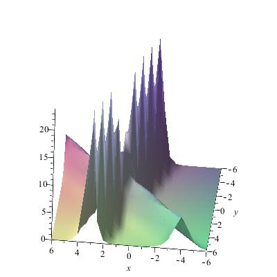
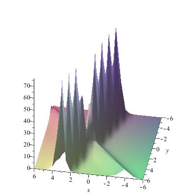
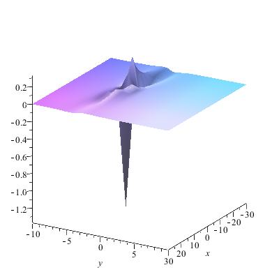
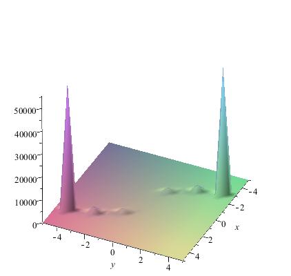
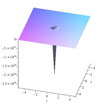
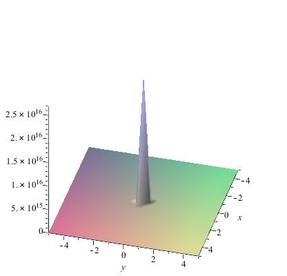
The pictures of solution (39) at different time are shown in Fig. 6 and Fig. 7. We note that, for the plus Boussinesq equation, the rational solution (39) is not a lump one. As shown in Fig.7, the surface is strange. This picture is obtained at special time and in special region, shows some form of energy ejection.
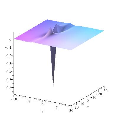
u(t=1),
v(t=1),
u(t=0),
v(t=0),
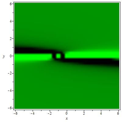
desityplot(u),
4 Discussions
If we choose and in (17) as and , where is defined by (7), and assume that and exit in some region of plane, then and in (19) satisfy the system
| (40) |
However, if functions and are not the delta functions, it is hard to give the explicit expression of in (20). As a result, the solution of the generalized Boussinesq (3) or the system (1) will not be obtained by the Dbar-approach.
We note that an alternative method only starting from (40) can be introduced to obtained the solution of Boussinesq (3). It is known that if is a special solution of (40), then
| (41) |
will solve the system (1). We note that the case of has been discussed in [6]. For example, a new particular solution of the system (1) can be given by choosing
| (42) |
where and are arbitrary constants. As shown in Fig. 8, there is a direction shift for the Boussinesq () wave propagation.
u(t=0),
v(t=0),
Abs(u)(t=0),
Abs(v)(t=0),
Acknowledgments
Project 11471295 was supported by the National Natural Science Foundation of China.
References
- [1] L. V. Bogdanov, S. V. Manakov, The non-local partmacr problem and (2+1)-dimensional soliton equations, J. Phys. A: math. Gen. 21 (1988) L537–L544.
- [2] R. R. Beals, R.; Coifman, Linear spectral problems, non-linear equations and the deltamacr-method, Inverse Problems 5 (1989) 87–130.
- [3] M. J. Ablowitz, P. A. Clarkson, Solitons, Nonlinear Evolution Equations and Inverse Scattering, Cambridge University Press, Cambridge, 1991.
- [4] B. G. Konopelchenko, Solitons in Multidimensions—Inverse Spectral transform Method, Word Scientific, Singapore, 1993.
- [5] M. J. Ablowitz, D. Bar Yaacov, A. S. Fokas, On the inverse scattering transform for the Kadomtsev-Petviashvili equation, Stud. Appl. Math. 69 (1983) 135–143.
- [6] T. Su, Explicit solutions for a modified 2+1-dimensional coupled Burgers equation by using Darboux transformation, Appl. Math. Lett. 69 (2017) 15–21.
- [7] H. P. McKean, Boussinesq’s equation as a Hamiltonian system, Adv. Math. Supp. Studies 3 (1978) 217–226.
- [8] H. P. McKean, Boussinesq’s equation on the circle, Commun. Pure Appl. Math. 34 (1981) 599–691.
- [9] V. A. Jurko, Solution of the Boussinesq equation on the half-line by the inverse problem method, Inverse Problems 7 (1991) 727–738.
- [10] C. Deift, P. Tomai, E. Trubowitz, Inverse scattering and the Boussinesq equation, Commun. Pure Appl. Math. 35 (1982) 567–628.
- [11] P. A. Clarkson, M. D. Kruskal, New similarity solutions of the Boussinesq equation, J. Math. Phys. 30 (1989) 2201–2213.
- [12] M. J. Ablowitz, R. Haberman, Resonantly coupled nonlinear evolution equations, J. Math. Phys. 16 (1975) 2301–2305.
- [13] P. J. Caudrey, The inverse problem for a general N N spectral equation, Physica D 6 (1982) 51–66.
- [14] P. J. Caudrey, The inverse problem for the third order equation , Phys. Lett. A 79 (1980) 264–266.
- [15] V. E. Zakharov, S. V. Manakov, S. P. Novicov, L. P. Pitaevsky, Theory of Solitons: The Inverse Scattering Method, Plenum Press, New York, 1984.
- [16] V. E. Zakharov, On stochastization of one-dimensional chains of nonlinear oscillations, Sov. Phys. JETP 38 (1974) 108–110.
- [17] L. V. Bogdanov, V. E. Zakharov, The Boussinesq equation revisited, Physica D 165 (2002) 137–162.
- [18] A. Himonas and D. Mantzavinos, On the initial-boundary value problem for the linearized Boussinesq equation, Stud. Appl. Math. 134 (2014) 62–100.
- [19] W. X. Ma, Complexiton solutions to the Korteweg-de Vries equation, Phys. Lett. A 301 (2002) 35–44.
- [20] W. X. Ma, A second wronskian formulation of the boussinesq equation, Nonlinear Anal. 70 (2009) 4245–4258.
- [21] W. X. Ma, K. Maruno, Complexiton solutions of the Toda lattice equation, Physica A 343 (2004) 219–237.
- [22] W. X. Ma, Complexiton solutions to integrable equations, Nonlinear Anal. 63 (2005) e2461–e2471.
- [23] M. A. Allen, G. Rowlands, On the transverse instabilities of solitary waves, Phys. Lett. A 235 (1997) 145–146.
- [24] A. M. Wazwaz, Variants of the two-dimensional Boussinesq equation with compactons, solitons, and periodic solutions, Comput. Math. Appl. 49 (2005) 295–301.
- [25] M. J. Xua, S. F. Tian, J. M. Tua, T. T. Zhang, Bäcklund transformation, infinite conservation laws and periodic wave solutions to a generalized (2+1)-dimensional Boussinesq equation, Nonlinear Anal. Real 31 (2018) 388–408.