Multiscale Bayesian State Space Model for Granger Causality Analysis of Brain Signal

Abstract

Modelling time-varying and frequency-specific relationships between two brain signals is becoming an essential methodological tool to answer theoretical questions in experimental neuroscience. In this article, we propose to estimate a frequency Granger causality statistic that may vary in time in order to evaluate the functional connections between two brain regions during a task. We use for that purpose an adaptive Kalman filter type of estimator of a linear Gaussian vector autoregressive model with coefficients evolving over time. The estimation procedure is achieved through variational Bayesian approximation and is extended for multiple trials. This Bayesian State Space (BSS) model provides a dynamical Granger-causality statistic that is quite natural. We propose to extend the BSS model to include the à trous Haar decomposition. This wavelet-based forecasting method is based on a multiscale resolution decomposition of the signal using the redundant à trous wavelet transform and allows us to capture short- and long-range dependencies between signals. Equally importantly it allows us to derive the desired dynamical and frequency-specific Granger-causality statistic. The application of these models to intracranial local field potential data recorded during a psychological experimental task shows the complex frequency based cross-talk between amygdala and medial orbito-frontal cortex.

keywords: À trous Haar wavelets; Multiple trials; Neuroscience data; Nonstationarity; Time-frequency; Variational methods

The published version of this article is

Cekic, S., Grandjean, D., Renaud, O. (2018). Multiscale Bayesian state-space model for Granger causality analysis of brain signal. Journal of Applied Statistics. https://doi.org/10.1080/02664763.2018.1455814

1 Introduction

In many neuroscientific experiments, data are recorded in an experimental situation where stimuli are presented at fixed times and are expected to induce a reaction. For psychologists and neuroscientists, being able to model and explain the dynamics of the functional and effective links between neural and behavioural signals recorded during the experiment is of primary interest. They often have strong prior hypotheses about these causal links and therefore need reliable statistical tools to draw valid conclusions.

1.1 Granger causality

The question of how to operationally formalize and test for causality is a fundamental and philosophical problem. A mathematical solution, which relies on the causal nature of predictability, was provided in the 60’s by the economist Clive Granger and was latter coined “Granger causality”. According to Granger [25], if a signal $X$ “Granger-causes” a signal $Y$, then the history of $X$ should contains information that helps to predict $Y$ above and beyond the information contained in the history of $Y$ alone. The axiomatic imposition of a temporal ordering is the crucial element that enables us to interpret such dependence as causal. The presence of this relation between $X$ and $Y$ will be referred to “Granger causality” throughout the text. In the 1960s, Granger [25] adapts the definition of causality proposed by Wiener [53] into a practical form and since that time Granger causality has been widely used in economics and econometrics. It is however only since last few years that it became popular in neuroscience, see Cekic et al. [12] for a recent review.

1.2 Existing methods and limits

In the context of linear Gaussian autoregressive models, for which the restrictions are Gaussianity and linearity, which imply stationarity in most cases, a common way to test for Granger causality between two series is to estimate a vector autoregressive model (VAR) and then test the significance of the off diagonal coefficients of interest [26, 34].

However, in neuroscience the data are usually nonstationary and this characteristic is moreover of interest. In the simplest case, the data are stationnary up to a particular point where the Gaussian process has been perturbed away from its stationary distribution (perhaps by some external intervention). We therefore want to derive a causality-statistic that allows us to capture the causal structure differentially for each time.

Basic causality statistic has therefore to be extended to the nonstationary case in order to be suitably applied in a neuroscience context, which can be achieved by letting the VAR model evolve in time.

Time-varying VAR model estimate implies three challenges: over-parametrization, model order selection and multiple trials.

The two widely used approaches allowing us to deal with the nonstationarity are the windowing approach, based on the locally-stationary assumption and the adaptive estimation approach, based on the slowly-varying assumption of the parameters (see Ding et al. [17], Schlögl [44] and [13]).

The windowing approach consists in estimating VAR models in short temporal sliding windows where the underlying process is assumed to be (locally) stationary (see Ding et al. [17] for a methodological tutorial of windowing estimation approach in neuroscience).

The windows size is a trade-off between the accuracy of the parameter estimates and the resolution in time. The choice of the model order is a delicate issue, and depends on the choice of the segment length. Some criteria have been proposed in order to optimized simultaneously the windows length and the model order [32].

The usual approach with multiple trials is to average the estimation or do a global optimization to get an overall estimation.

In Cekic [10] we found that this windowing methodology presents several limits. First, the improvement of the time resolution implies short time-windows and so few residuals for assessing the quality of the fit. In addition the size of the temporal windows is subjective (even if it depends on a criterion) as is the overlap between the time-windows. The order of the model in turns depends on the size of the windows and so the quality of the estimation strongly relies on several subjective parameters.

The adaptive estimation approach consists on estimating a different model at each time, where the observations at time $t$ are expressed as a linear combination of the past with coefficients evolving slowly over time. The differences between the methods consist on the way the transition and the update from coefficients at time $t$ to those at time $t+1$ are processed [see 44].

All these adaptive estimation methodologies depend on a quantity that acts as a tuning parameter and defines the relative influence of past values and innovation noise on the recursive estimation. Generally this free tuning parameter determines the speed of adaptation as well as the smoothness of the time-varying VAR parameter estimates. The algorithms are very sensitive to this tuning parameter [44] and therefore the estimation quality strongly depends on it. The “ad-hoc” nature of this tuning parameter is obviously a problem in term of statistical inference and this issue was not raised in the development of these algorithms coming from the engineering field. The model order and the tuning parameters are usually optimized together by a Mean Square Error criterion [45].

Kalman filtering algorithm [29] can be used in order to estimate time-varying VAR models when we express it in a state space form [1, 4].

If the transition matrix and variance-covariance matrices of the observed and state equation are known, the Kalman smoother algorithm gives the best linear unbiased estimator for the state vector [29], which in this specific case contains the time-varying VAR coefficients. In the engineering and neuroscience literature, these matrices are systematically set to fixed values or estimated through some “ad-hoc” estimation procedure (see Schlögl [44] and Hesse et al. [27], Arnold et al. [1] for applications in neuroscience). There is moreover the very important issue of model order selection which becomes very tricky with model complexity and the plurality of the trials.

1.3 Neuroscience data specificities

Our model has to be applied to experimental neuroscience data, whose intrinsic specificities must be taken into account in its development. Therefore, in order to derive a suitable dynamical causal statistic, we need a model that allows us to get a reliable estimate of the dynamical VAR coefficients based on several trials and, last but not least, that also allows us to capture short- and long-range causal dependencies between signals due to specific frequency characteristics of the data.

1.4 Proposal

Faced with data with a time-varying structure (like neuroscience data), none of the above methods relies on a tailored statistical model that provides satisfying estimation and inference procedures and proposes a solution to deal with short and long range causal dependencies potentially present in the data.

We propose a new methodology for suitably modelling multivariate nonstationary time series in order to get a reliable Granger-type dynamic causal statistic. It is based on a linear Gaussian vector autoregressive (VAR) model with coefficients evolving over time according to a linear dynamical system. Given that this model is strongly over-parametrized, we propose to place it in a Bayesian framework and to use the variational method to estimate all the densities. This variational Bayesian methodology [6] estimates all the necessary quantities. The Bayesian nature of the model moreover offers a natural criterion for model order selection. In Section 2, we describe our Bayesian state space (BSS) model and discuss its technical specificities and the estimation procedure. We extend it to deal with multiple trials (or epochs), in a proper manner for the estimation and the inference procedure (section 3.3). In Section 4, we propose an additionnal extension of the BSS model, called the multiscale Bayesian state space (MSBSS) model, which is based on the à trous multiscale wavelet transform. The latter approach has never been used in this context of time-varying VAR coefficient estimate and we will show that it allows better estimate of short- and long-range specific dependencies between recorded signals and offers a very simple way to deal with time-frequency uncertainty bounds. In Section 5, we will present a Bayesian dynamical Granger-causality statistic based on the time-varying estimated VAR coefficients and in Section 6, we present simulation studies to assess our proposed methodology. Finally, we present in Section 7 the results of the application of the method to intracranial local field potential recorded during a psychological experiment in specific brain areas, namely in the amygdala and orbitofrontal cortex.

2 The Bayesian State Space Model

We propose to write the dynamic VAR model in a state space form with an observation equation in which the dynamic VAR coefficients are driven by the state equation [this modelling proposal was previously made by 9]. This leads to the following system of equations:

$$\left\{\begin{aligned} \varphi_{t+1}=A\varphi_{t}+w_{t}\quad&w_{t}\sim{\mathcal{N}_{k}(0,Q)}\\ Z_{t}=C_{t}\varphi_{t}+v_{t}\quad&v_{t}\sim{\mathcal{N}_{d}(0,R)}\\ \end{aligned}\right.\quad\text{with}\quad\begin{cases}\varphi_{t}&=\operatorname{vec}[\vartheta_{1(t)},\vartheta_{2(t)},..,\vartheta_{p(t)}]^{\prime},\\ Z_{t}&=(Y_{t}\;X_{t})^{{}^{\prime}},\\ C_{t}\varphi_{t}&=\sum\limits_{j=1}^{p}\vartheta_{j(t)}(Y_{t-j}\;X_{t-j})^{{}^{\prime}},\end{cases}$$ (1)

where $Z_{t}=(Y_{t}\;X_{t})^{{}^{\prime}}$ is the value of the $d=2$ signals at time $t$, $\vartheta_{j(t)}$ are the time-varying VAR coefficients (up to order $p$) and the vector $\varphi_{t}$ of size $k=pd^{2}$ contains all the time-varying VAR coefficients that have to be estimated for the time $t$. The matrix $A$ is the transition matrix of the state vector $\varphi_{t}$, $Q$ is the $k\times k$ variance-covariance matrix of the state equation, and $R$ is the $d\times d$ variance-covariance matrix of the observation equation. We will use the notation $\varphi_{1}^{T}$ and $Z_{1}^{T}$ to denote the entire set of values from $t=1$ to $t=T$. Although the state equation seems to be only a first-order autoregression, note that the vectors $\varphi_{t}$ and $\varphi_{t-1}$ contain all the coefficients up to order $p$, and therefore the direct dependency of $\varphi_{t}$ on past values is actually unlimited (and driven by the choice of the order $p$). This formulation is actually similar to the state-space representation of AR(p) or ARMA(p,q) models (see e.g. [4] examples 12.1.4-5)

With a slight abuse of notation, we can write $p(Z_{t}|C_{t},\varphi_{t},R)=\mathcal{N}_{d}(C_{t}\varphi_{t},R),\\ p(\varphi_{t}|A,\varphi_{t-1},Q)=\mathcal{N}_{k}(A\varphi_{t-1},Q)$ and $p(\varphi_{1})=\mathcal{N}_{k}(\mu_{1},\Sigma_{1})$, which are respectively the observation, the state and the initial state densities.

Given the Bayesian framework, we are interested in obtaining the posterior distribution of the unknowns of this model. In simple cases, these distributions can be obtained analytically but here, the curse of dimensionality makes the computation intractable and forces us to rely on approximation techniques.

2.1 Variational Bayes

Variational approximation was applied to the linear Gaussian state space model in Ghahramani and Beal [21] and Cassidy [9], and more recently in Luessi et al. [33]. This approximation methodology has been extensively explored and used during the past years; see for example Titterington [49], Beal [6], Ormerod and Wand [38] and Fox and Roberts [18]. It is not widely known within the statistical community dominated by Monte Carlo and Laplace approximation methods but is however much faster than Monte Carlo, especially for large models, and allows us to deal with models containing a very large amount of parameters (see Friston et al. [19] for a comparison of variational and Laplace approximations).

For sake of clarity, we will define the set of unknown parameters as $\Omega_{1}^{b}$, so the full set of unknowns for model (1) is $\{\varphi_{1}^{T};\Omega_{1}^{b}\}$.

The target quantity is the posterior distribution of the parameters which is an intractable integral of very high dimension. The variational approach allows us to approximate this posterior density $p(\varphi_{1}^{T},\Omega_{1}^{b}|Z_{1}^{T})$ by a variational posterior density $q(\varphi_{1}^{T},\Omega_{1}^{b}|Z_{1}^{T})$ that will be selected to be optimal according to the Kullback–Leibler distance dissimilarity criterion [6] (see Appendix A for further details on variational Bayesian approximation).

2.2 Mean-field approximation

Variational Bayesian methodology allow the approximating density $q(\varphi_{1}^{T},\Omega_{1}^{b}|Z_{1}^{T})$ to factorize over groups of parameters. The researcher has the choice here, but the explicit link between the $\varphi$’s in equation 1 urge not to factorize $\varphi_{1}^{T}$. The less intricate links between $\varphi_{1}^{T}$, $A$, $Q$ and $R$ allow for the following factorization (see Figure A.1 from the supplementary material)

$$q(\varphi_{1}^{T},\Omega_{1}^{b}|Z_{1}^{T})=q(\varphi_{1}^{T}|Z_{1}^{T})\prod_{j=1}^{b}q(\Omega_{j}|Z_{1}^{T}).$$ (2)

Note that it may lead to serious degradation in the resulting inference if unsatisfied [38, 49, 6].

2.3 The variational evidence lower bound

As presented in details in Appendix B, the variational Bayesian methodology provides a quantity F that is a lower bound for the evidence of the model and that can be computed efficiently. This leads to a natural criterion for model order selection which is crucial to estimate our strongly over-parametrized time-varying VAR model. We can therefore perform model selection by comparing the F quantities computed for each model order $m_{p}$ and select the model that exhibits the highest $\text{F}_{m_{p}}$. The specific analytic form of $\text{F}_{m_{p}}$ for our model is derived in Appendix B.

3 Model specification

We will now describe the fully hierarchical Bayesian model that we propose.

The optimal form for $q^{*}(\varphi_{1}^{T}|Z_{1}^{T})$ and $q^{*}(\Omega_{1}^{b}|Z_{1}^{T})$ of course depends on the choice of the prior distributions $p(\varphi_{1}^{T})$ and $p(\Omega_{m})$. However, the analytical form of $q^{*}(.|Z_{1}^{T})$ will be of the same distributional form as the prior distributions $p(.)$ if the complete-data likelihood $p(\varphi_{1}^{T},Z_{1}^{T}|\Omega_{1}^{b})$ is part of the exponential family and if the hidden and parameter prior distributions $p(\varphi_{1}^{T})$ and $p(\Omega_{1}^{b})$ are conjugate to this complete-data likelihood (this condition is known as “conjugate exponential”, see Beal [6]).

Recalling the model (1), the complete data likelihood $p(\varphi_{1}^{T},Z_{1}^{T}|\Omega_{1}^{b})$ is Gaussian. We will now describe the model by defining conjugate priors over the model parameters.

3.1 Prior distributions

3.1.1 Prior for $\varphi_{1}^{T}$

The state space structure of the model (1) leads to the conditional prior distributions for the hidden state $\varphi_{1}^{T}$ defined in Section 2 and the prior mean $\mu_{1}$ and variance $\Sigma_{1}$ for $\varphi_{1}$ are set to $1_{k}\times 0$ and $I_{k}\times 0.1$ respectively.

3.1.2 Prior for $\Omega_{1}=\{A,\mathbf{\alpha},\mathbf{\delta}\}$

We propose a diagonal structure for the $A$ matrix, meaning that a specific causal coefficient at time $t$ will only depend on its own past value plus a white noise and not on the past values of other VAR coefficients. This assumption seems reasonable in terms of brain connectivity, where the dynamic of a particular causal input can be assumed to be driven by its own trajectory and not by that of other causal or auto-causal inputs. To satisfy the conjugacy condition explained in details in Appendix A, We place a Gaussian prior on each diagonal entry of the $A$ matrix:

$$p(A|\mathbf{\alpha})=\prod_{i=1}^{k}\mathcal{N}_{1}(A_{ii}|m_{A_{ii}},\alpha_{i}),$$ (3)

where $\alpha_{i}$ is the hyperparameter variance of the specific diagonal element $A_{ii}$ whose distribution will be discussed below. We choose to impose a conservative prior for $A$ by setting each location hyperparameter $\{m_{A_{ii}}\}_{i=1}^{k}$ to $0.9$.

As we have no subjective input for the variances $\alpha_{i}$, it is desirable to have priors that exhibit very little information. The main recommendation in Gelman [20] is to use half-t priors on standard deviation parameters to achieve arbitrarily high noninformativeness. The definition of the half-t distribution can be found e.g. in Wand et al. [50]. They showed that the half-t distribution can be written as a scaled mixture of inverse-gamma distributions. So the half-t prior is obtained for each $\alpha_{i}^{0.5}$ element through the auxiliary variable construction

$$\begin{split}p(\alpha_{i}|\delta_{i})=\mathcal{IG}(c_{p_{i}},b_{p_{i}})=\mathcal{IG}(\frac{1}{2},\frac{1}{\delta_{i}}),\\ p(\delta_{i})=\mathcal{IG}(\kappa_{p_{i}},\beta_{p_{i}})=\mathcal{IG}(\frac{1}{2},\frac{1}{D_{i}^{2}}),\quad i=1,\dots,k,\end{split}$$ (4)

which ensures that $p(\alpha_{i}^{0.5})=\text{Half-t}(1,D_{i})$. The hierarchical representation in equation (4) respects the conditional conjugacy condition due to the conjugacy properties of the inverse-gamma distribution.

By its noninformativeness property, this half-t prior choice will let each variance element $\{\alpha_{i}\}_{i=1}^{k}$ get an appropriately high or low value, thereby allowing them to play the role of shrinkage parameters for the distribution of $A_{ii}$. In our specific case, it will allow us to be conservative and to tend to avoid an erroneous causality assessment.

3.1.3 Prior for $\Omega_{2}=\{Q,a_{q}\}$

The accuracy of the Markovian conditional distribution followed by the VAR coefficients $\varphi_{t}$ is established through the variance-covariance matrix $Q$. Throughout this work we assume that this matrix is diagonal (for the same theoretical reason discussed for the $A$ matrix) and that all its elements are equal. In fact there is no reason to assume that the variability of one VAR coefficient is different from that of another. This choice is also motivated by the concern to limit the number of parameters to estimate.

In order to satisfy the conjugacy conditions and for the same theoretical reason mentioned earlier, we set the same weakly-informative half-t prior distribution for the single standard deviation parameter $Q_{ii}^{0.5}$ of the diagonal $Q$ matrix:

$$\begin{split}p(Q_{ii}|a_{q})=\mathcal{IG}(n_{p},d_{p})=\mathcal{IG}(\frac{1}{2},\frac{1}{a_{q}}),\quad p(a_{q})=\mathcal{IG}(a_{qp},b_{qp})=\mathcal{IG}(\frac{1}{2},\frac{1}{A_{q}^{2}}),\end{split}$$ (5)

which again ensures that $p(Q_{ii}^{0.5})=\text{Half-t}(1,A_{q})$.

3.1.4 Prior for $\Omega_{3}=\{R,a_{r}\}$

The variance-covariance matrix $R$ of the observed equation is not supposed to be diagonal due to the theoretical interdependence between brain signals modelled in the system.

We impose for $R$ a generalisation of the multivariate case of the Half-t prior used for $\alpha$ and $Q_{ii}$. Huang et al. [28] derived this prior and explained that with a suitable hyperparameter choice, it induces an Half-t distribution for each standard deviation term corresponding to the diagonal of $R$, as well as a marginal uniform distribution for all correlations. Explicitly we have

$$\begin{split}p(R|a_{r_{1}},\dots,a_{r_{d}})&=\mathcal{IW}_{d}\big{(}r_{p},B_{p})=\mathcal{IW}_{d}\big{(}\nu+d-1,2\,\nu\,\text{diag}[\frac{1}{a_{r_{1}}},\dots,\frac{1}{a_{r_{d}}}]\big{)},\\ p(a_{r_{i}})&=\mathcal{IG}(a_{pr},b_{pr})=\mathcal{IG}(\frac{1}{2},\frac{1}{A_{R}^{2}}),\qquad i=1,\dots,d,\end{split}$$ (6)

where $\text{diag}()$ denotes a diagonal matrix. This hierarchical structure ensures that each diagonal element $R_{i,i}$ is distributed as $p(R_{i,i}^{0.5})=\text{Half-t}(\nu,A_{R})$, and the particular choice of $\nu=2$ leads to marginal uniform distributions over $[-1;1]$ for all correlation terms [28].

Lastly, we note that the selected prior distributions impose the choice of hyperparameters $D_{1},\dots,D_{k}$, $A_{q}$, $\nu$ and $A_{R}$. We will choose $\nu=2$ for the uniform property to hold. For the remaining hyperparameters, the larger they are the less informative the priors are. We follow Menictas and Wand [36] and set them to $10^{5}$.

3.2 Update equations

The variational Bayesian iterative algorithm and optimal posterior distributions are based on the results presented in Appendix A and factorization chosen in Section A.0.2. The optimal variational posterior distribution for the hidden state sequence $\varphi_{1}^{T}$ (Variational E-Step) is multivariate Gaussian at each time $t$:

$$q^{*}(\varphi_{t}|Z_{1}^{T})=\mathcal{N}_{k}(\varphi_{t}|\mu_{t},\Sigma_{t}),$$ (7)

where the sufficient statistics $\{\mu_{t};\Sigma_{t}\}_{t=1}^{T}$, as well as the cross-moments
$\{\mu_{t}\mu_{t-1};\Sigma_{t,t-1}\}_{t=2}^{T}$, are obtained by the Kalman–Rauch–Tung–Striebel (KRTS) smoother algorithm [29, 30], applied to an augmented system of equations, see Appendices C, D and E. All the derivations for the Variational M-steps can be found in Appendices F, G, H, I, J, K and L.

3.3 Multiple trials

One important contribution of the present article is to show that our model can be modified to deal with $N$ conditionally independent sequences $\{{Z_{1}^{T}}_{(j)}\}_{j=1}^{N}$ which are supposed to have the same hidden state. This reflects the case that arises during an event-related experimental paradigm, where many trials on the same condition are measured.

In Beal [6] and Cassidy [9], this extension is treated by first estimating the necessary sufficient statistics for each sequence independently in the E-step, and then by averaging these statistics to get only one set of sufficient statistics, which is representative of the entire set of independent sequences before performing the M-step. However this approach does not take into account the complex dependence of the variational posterior $q(\varphi_{1}^{T}|\{{Z_{1}^{T}}_{(j)}\}_{j=1}^{N})$ on the whole dataset $\{{Z_{1}^{T}}_{(j)}\}_{j=1}^{N}$. In fact, all the computations done so far can be adapted to multiple trials. A detailed derivation of the model and related variational posteriors distributions in a multiple trials setting can be found in Appendix M.

4 The Multiscale Bayesian State Space Model

In a neuroscience context, an important limitation of many models, including the BSS model, is the inability to capture both the short- and long-range possible causal dependencies between signals. Causal interactions in a neuroscientific experiment context may not be instantaneous, but delayed over a certain time interval $(\upsilon)$ that must be subjectively chosen depending on the research hypothesis. Another important subjective parameter is the time-lag ($\tau$), that determines the interval between two data points As shown in Barnett and Seth [5] and Solo [48] these choices strongly influence classical Granger statistics in their ability to detect causalities, whereas the result should be as invariant as possible to arbitrary choices like the chosen sampling frequency or added time-lag in the prediction model.

Based on these considerations, and because Granger causality is based on predictive ability, if the auto-causal information contained in the history of the predicted signal $Y_{t}$ in model (1) is not well represented in $C_{t}$, the Granger-causality evaluation, which is based on the predictability improvement of $Y_{t}$ by adding the information contained in the history of the second variable $X$, may be spuriously assessed as significant. On the other hand, if the predictive ability of the history of the causal signal $X$ is not informative enough, we can miss some crucial information about causal interdependencies between signals $Y$ and $X$.

We propose a new solution that has the ability to appropriately select the short- and long-term causal histories of $Y$ and $X$ by combining the BSS model with the à trous multiscale decomposition methodology and that remains within the conjugate exponential framework [41].

4.1 The à trous Haar wavelets transform

For that purpose, we will perform the à trous multiscale decomposition of signals $Y_{t}$ and $X_{t}$ contained in $Z_{t}$ in model (1), in order to use these quantities as predictive histories in the matrices $\{C_{t}\}_{t=1}^{T}$. The reader is referred to Renaud et al. [41] and references therein for a complete overview of the method. We define $w^{y}_{j,t}$ as the à trous wavelet coefficient of the signal $Y$ at time $t$ for scale $j$. Since we will use the à trous wavelet coefficients for prediction, they should not be based on future values and the only family that satisfies this constraint is the à trous Haar wavelet transform. Then $S_{j+1}(t)=[S_{j}(t)+S_{j}(t-2^{j})]/2,\quad w_{j+1}(t)=S_{j}(t)-S_{j+1}(t),\quad t=1,\ldots,T,\quad j=1,\ldots,J$, where the finest scale is the original series $S_{0}(t)=Y_{t}$.

4.2 The multiscale Bayesian state space model

Based on the derivation in Section 4.1, we can modify the VAR model in equation (1). We keep the quantity to predict $Y_{t}$ in the time domain, but the histories of the series $Y$ and $X$ will equal the à trous Haar wavelet transforms of series $Y_{t}$ and $X_{t}$ respectively. We can therefore define the set $C_{t}^{w}$ that contains the decompositions of the histories of series $Y_{t}$ and $X_{t}$ as

$$C_{t}^{w}= {\{w^{y}_{j,t-1-2^{j}(k-1)}\}_{j=1,\ldots,J,k=1,\ldots,p_{j}}},\{s^{y}_{J,t-1-2^{J}(k-1)}\}_{k=1,\ldots,p_{J+1}},$$ (8)

$$\{w^{x}_{j,t-1-2^{j}(k-1)}\}_{j=1,\ldots,J,k=1,\ldots,p_{j}},\{s^{x}_{J,t-1-2^{J}(k-1)}\}_{k=1,\ldots,p_{J+1}},$$

and therefore adapt equation (1) replacing $C_{t}$ with $C_{t}^{w}$.

In particular, we underline that for any $J$, for a suitable choice of $p_{1},\dots,\\ p_{J+1}$, $C_{t}^{w}$ is an orthogonal transform of $C_{t}$ and therefore in this specific case BSS and MSBSS models are equivalent. For any choice of the $p$’s, all results in Section 2 and all the estimation procedures in Section 3 can be applied. The only difference is that the matrix $C_{t}$ is replaced by $C_{t}^{w}$, and that the dimension of $\varphi_{t}$ is changed accordingly. The model order $p_{j}$ for the different scales as well as the number of scales $J$ to be taken in the model must now be selected. As argued in Renaud et al. [41], the relative non-overlapping frequencies used in each scale motivate an independent selection of the model order $p_{j}$ for each scale. Defining a maximal scale decomposition $J_{\text{max}}$ and a maximum model order for each scale $p_{\text{max}}$, the model order selection procedure set in Section A.1 is iteratively applied to select $p_{j}$ in a stepwise manner for each scale from 1 to $J_{\text{max}}$. The free-energy quantities related to the $J_{\text{max}}$ models are then compared and the $J$ that exhibits the highest free energy is selected. The model order for the smooth $p_{J+1}$ is finally selected.

This à trous extension can thus be viewed as a generalisation of the BSS model that contains information relative to the frequencies. Each wavelet scale indeed is directly related to a specific frequency band and the resulting dynamic Granger causality statistic is therefore directly interpretable in terms of frequencies (see Section 7).

5 Bayesian Granger-Causality Statistic

Based on the model proposed in this article, a necessary and sufficient condition for $X_{t}$ not to be Granger-causal for $Y_{t}$ at a given time $t$, is that each element of the subset $\widetilde{\varphi_{t}}$ of $\varphi_{t}$, that contains all the causal coefficients of interest, equals zero.

The most appropriate approach to evaluate the compatibility of this type of hypothesis with the data would be to compute for each time $t$ a Bayes factor between the VAR model under the restriction $\widetilde{\varphi_{t}}=0$ for just one value of $t$ ($M_{1}^{t}$) and the VAR model without restrictions ($M_{2}^{t}$). For each $t$, this would requires the computation of the evidence of model $M_{1}^{t}$, which seems untractable: one would need a Markovian process for $\varphi_{t}$ that is conditionned (sort of bridge) on the restriction that $\widetilde{\varphi_{t}}=0$ for just one given $t$. At the very least, one would need to estimate a different (conditional) model for each $t$ and compute its free energy. Additionnaly, we have no guarantee that the free energy approximation is of the same magniture for all these models.

We will use a simpler approach that rely only on the posterior density of the (unconditional) model. The use of highest posterior density (HPD) regions for Bayesian testing was introduced in Box and Tiao [7] and used in the Bayesian literature, as for example in Kim and Press [31] and West and Harrison [52, p. 280]. For a given time $t$, consider the sub-vector $\widetilde{\varphi_{t}}$ and let $c$ be its dimension. A suitable partition of the posterior parameters $\mathbf{\mu_{t}}$ and $\Sigma_{t}$ gives the marginal posterior density $q(\widetilde{\varphi_{t}}|Z_{1}^{T})=\mathcal{N}_{c}(\widetilde{\mu_{t}},\widetilde{\Sigma_{t}})$. The contribution of each element of $\widetilde{\varphi_{t}}$ to the prediction of $Y_{t}$ may be assessed by considering the compatibility in this marginal posterior with the value $\widetilde{\varphi_{t}}=\widetilde{\varphi_{0_{t}}}$, where $\widetilde{\varphi_{0_{t}}}$ is a zero vector of dimension $c$. The question is therefore to know whether the parameter point $\widetilde{\varphi_{t}}=\widetilde{\varphi_{0_{t}}}$ is included in the highest posterior density region (HPD) of size $1-\alpha$. This happens if and only if $(\widetilde{\varphi_{0_{t}}}-\widetilde{\mu_{t}})^{\prime}\widetilde{\Sigma_{t}}^{-1}(\widetilde{\varphi_{0_{t}}}-\widetilde{\mu_{t}})<k$, where $k$ is the $1-\alpha$ quantile of the standard $\chi^{2}$ distribution with $c$ degrees of freedom. As stated in Box and Tiao [7, p. 125], it follows that the parameter point $\widetilde{\varphi_{0_{t}}}$ is covered by the HPD region of content $1-\alpha$ if and only if $\mathrm{Pr}\{p(\widetilde{\varphi_{t}}|Z_{1}^{T})>p(\widetilde{\varphi_{0_{t}}}|Z_{1}^{T})|Z_{1}^{T}\}\leq 1-\alpha$. Equivalently, we can search the region of minimum coverage that contains $\widetilde{\varphi_{0_{t}}}$.

The above approach gives only pointwise evaluations (i.e., for a given time $t$). When jointly testing a set of values for a complete time, frequency or time-frequency connectivity map, it is important to suitably correct the significance threshold for multiple comparisons. We do not correct it in Section 6 as we are interested in the separate evaluation for each time but we do for the application in Section 7.

6 Assessment of Accuracy

We now turn our attention to the accuracy of variational Bayesian inference for our model (1) under the mean-field assumption described in Section A.0.2 and priors discussed in Section 3. We provide here a study of the quality of variational Bayesian estimate for model order selection and Granger causality detection. The first simulation study in Section 6.2 evaluates the ability of the BSS and MSBSS models to detect Granger causalities between two signals and in Section 6.2, we present a systematic comparison between the proposed BSS and MSBSS models and the windowing approach in term of Granger causality detection ability. Note that a Monte-Carlo type of simulation is not feasible due to the very large amount of unknown parameters of our model and so direct comparison of the obtained variational posterior with true posterior density was unfortunately not feasible.

6.1 Practical implementation

To initialize the BSS and the MSBSS model algorithms, we run 10 iterations of the simple EM algorithm [47]. We thereby obtain reliable starting values for $\{\varphi_{1},\Sigma_{1},\Omega_{1}^{b}\}$ under initial conditions defined in Section 3. We then iteratively update the parameters of the variational approximate posteriors through the Variational Bayes EM until the relative free-energy criterion described in Section A.1 between two consecutive iterations changes less than a tolerance value that we choose here to be equal $10^{-2}$ for the model order selection study and to $10^{-4}$ for the Granger causality detection study following Menictas and Wand [36].

6.2 Granger-causality detection

We will now assess the ability of the proposed models BSS and MSBSS to detect Granger causality. We simulated signals with parameters that vary slowly in time, which is a reasonable simulation of neuroscientific data. It will show how the method performs with data that are not generated according to the model. The simulation consists in $50$ replications of a bivariate BSS model but with hidden variables $\varphi_{1}^{T}$ that evolve slowly and deterministically through time. Based on these deterministic $\varphi_{1}^{T}$, data are generated from the observed equation in model (1). The simulations were carried out for model orders $\{1;2;4;8\}$, series lengths $\{500;1000;2000\}$, number of trials $\{1;10\}$ and also for different values of the causal parameter $\{1;0.8;0.6;0.4;0.2\}$ in order to see the limits of the methods. The simulations for the causal parameter values $\{0.8;0.6;0.4;0.2\}$ were carried out for all model orders and number of trials, but only for a series length of $500$ time points (which is the case where the method will break first).

The $R$ matrix was fixed to the $I_{d}\times 0.1$ values and the slowly-varying parameters are all set to zero except for the entries related to the causal parameters $\{\varphi_{2\rightarrow 1}\}_{t=1}^{T}$ and $\{\varphi_{1\rightarrow 1}\}_{t=1}^{T}$ for order $p$. The values of the simulated parameters can be seen on the two panels (which are identical) on the top of Figures in Appendix N. Signals were simulated with normal and non-normal errors. Additional simulation settings and additional results are available in [11]

Data generated with slowly-varying parameters and normal errors

Concerning the MSBSS model, for each of the $50$ simulation, the model order $p_{j}$ for the different scales as well as the number of scales $J$ to be taken in the model are selected as described in Section 4. The maximum number of scale was set at $4$ and the maximal model order per scale at $5$. In multiple trial scenarios, the number of scales as well as the model order selection procedure was carried on one single trial only (for computational simplicity). Estimation procedure is always conditioned on the same number of time points, allowing us to compare the models. The Granger-causality detection capability of a method is quantified by the true negative rate (TNR) and the true positive rate (TPR). For each time, TNR is the percentage of the $50$ simulations for which the $95$% HPD region defined in Section 5 contains the causal statistic when it must actually contain it, and TPR is the percentage of the $50$ simulations for which the $95$% HPD region does not contain the causal statistic when it should not. Secondly, the BSS model is estimated with the true model order (oracle order) and the relative TNR and TPR are computed for that model. Finally, for the BSS model, the model order $p$ is selected with the free-energy criterion as described in Section A.1 and the model is estimated based on this selected order $p$. The relative TNR and TPR are calculated.

The causality detection ability for the BSS model with estimated model order is not shown in the results, because the model order was selected correctly by the free-energy criterion for each simulation (the causality detection ability is thus exactly the same as this for the BSS model with oracle order).

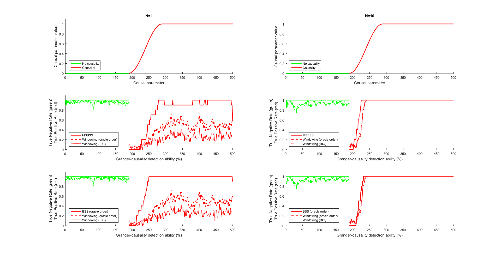
Figure 1: Granger-causality detection ability for order $4$, series length $500$ and causal parameter $1$. Top graphs show the value of the true parameters. Middle graphs display the true positive and true negative rates for the MSBSS model estimation, the windowing estimation with the true model order estimate (oracle) and the windowing estimation with the model order selected based on the BIC criterion. Bottom graphs display the true positive and true negative rates for the BSS model estimation, the windowing estimation with the true model order estimate (oracle) and the windowing estimation with the model order selected based on the BIC criterion.

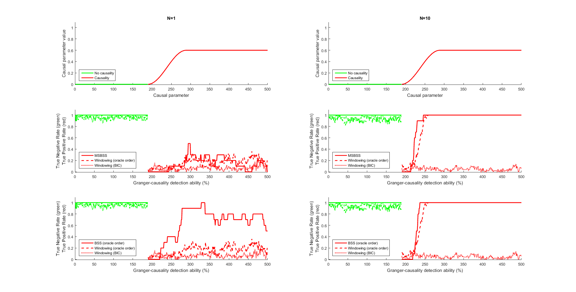
Figure 2: Results for the same settings as Figure 1 except for the causal parameter which is set to $0.6$

Figures 1 and 2 show Granger-causality detection accuracy for a model order $4$, series length of $500$ and causal parameter equal to $1$ and $0.6$ respectively. By construction, the causality arises between times $190-500$, as shown in the two graphs on the top of the figures. For Figure 1, the BSS model performs slightly better than the MSBSS model with $1$ trial and both methods yield very similar results, correctly recovering the underlying directional influences with $10$ trials. One can observe that the causality detection evolves as the causal parameter changes from zero to one. The TPR is indeed gradually increasing as the parameter changes from zero to one, slightly faster for the BSS than for the MSBSS model for $N=1$, and identically for $N=10$. For Figure 2, with such a low causal parameter, the TPR related to the MSBSS model is worse than the one related to the BSS model for $1$ trial, but both method perform very well with $10$ trials although the causal parameter is low.

Figures for Granger-causality detection accuracy related to all other model orders, series lengths and causal parameter values for normal errors are given in Appendix N. Globally, for a causal parameter that equals $1$, the MSBSS and the BSS models show very good Granger-causality detection accuracy in terms of TPR and TNR for $1$ and $10$ trials. The only cases which display poorer results are the causality detection for the MSBSS model with $1$ trial for model order $2$ and series length $500$, $1000$ and $2000$. When the causal parameter value decreases, the causality detection ability decreases as well. Poorer causality detection results are globally observed for a causal parameter from $0.6$ to $0.2$ for $1$ trial and for a causal parameter value of $0.2$ for $10$ trials, especially for the MSBSS model.

Data generated with slowly-varying parameters and non-normal errors

We also simulated data with the same settings as above, except for the observation equation errors which are here multivariate t-distributed with parameters $\nu=5$ and $R=I_{d}\times 0.1$. All graphical results can be found in Appendix N. Globally, the detection accuracy remains satisfactory with data generated with non-normal errors. The Granger-causality detection ability of the proposed methods is therefore robust to this model assumption departure.

Comparison with the windowing approach.

We will now compare our proposed models (BSS and MSBSS) with the windowing approach. The comparison is performed on data generated with slowly-varying parameters with normal errors as explained in Section 6.2. Simulations are performed for model orders $\{1;2;4\}$, series length $500$, number of trials $\{1;10\}$ and causal parameter values $\{1;0.8;0.6;0.4;0.2\}$. Data are fitted using the sliding window methodology proposed in Ding et al. [17]. The overlap parameter between the time-windows is chosen to be equal to $1$ time point and the subjective windows size is chosen to be equal to $15$ time points. The model estimation procedure is performed using the Viera–Morf algorithm implemented in BSMART [15] and GCCA toolboxes [46]. A first estimate was obtained with the true model order (oracle). For a second estimate, the model order selection is performed by considering the mode of the optimal model order calculated in each temporal window based on the Bayesian Information Criterion (BIC) as proposed in the BSMART toolbox [15], in the GCCA toolbox [46] and in the SIFT toolbox [37]. Based on the estimated models, a time-domain Granger-causal $F$ statistic is computed in each temporal window and its significance is assessed through the asymptotic $F$ distribution (see [15] and [46] for further details).

In Figures 1 and 2, the dash and the dot lines represent the results for the windowing approach. For Figure 1, the MSBSS and the BSS models perform much better than the windowing approach with the true model order and with the model order selected based on the BIC criterion for $1$ trial. MSBSS and the BSS models detect the causality faster than the windowing approach with $10$ trials. The TPR is worse for the windowing estimation than for the MSBSS and the BSS models for both $1$ and $10$ trials. For the case with a low causal parameter (Figure 2), the windowing estimation with oracle order performs almost identically as the MSBSS model and performs much worse than the BSS model for $1$ trial. MSBSS and the BSS models detect the causality faster than the windowing approach with oracle order with $10$ trials. The windowing estimation with the model order selected based on the BIC criterion display very poor detection accuracy for $1$ and for $10$ trials.

All other graphical results related to the windowing estimation procedure can be found in Appendix N. Globally, for the simulations with $1$ trial, the model order selection procedure based on the BIC performs well for order $1$ and is inaccurate for orders $2$ and $4$ and the related Granger-causality detection fails. One can observe that the causality detection evolves as the causal parameter changes from zero to the maximal value of the causal coefficient. For the simulations with $1$ trial, the windowing estimate detects the causality pattern globally slower than the MSBSS and the BSS models, whereas the TNR remains almost identical. When the value of the causal parameter decreases, the TPR for the MSBSS model decreases as well and becomes worse than the TPR for the windowing estimate in some cases (e.g., for the causal parameter $0.6$ and model order $1$). The TPR for the BSS model estimate decreases with the value of the causal parameter as well, but its TPR is always better than the TPR for the windowing estimation procedure. When the causal parameter equals $0.2$, however, the MSBSS and BSS model estimates do not detect anything whereas the windowing approach displays a TPR around $5-10$%.

For the simulations with $10$ trials, the model order selection procedure based on the Bayesian Information Criterion performs well overall. Windowing estimate (with model order selected by the BIC and oracle model order) globally detects the causality pattern slower than the MSBSS and the BSS models, whereas the TNR is almost identical everywhere. When the value of the causal parameter decreases, the model order selection procedure based on the BIC performs less well and its TPR degrades even more than the one for the MSBSS and the BSS models (e.g., for order $2$ and causal coefficient $0.4$ and $0.2$ and for order $4$ and causal coefficient $0.6$, $0.4$ and $0.2$).

7 Application

We will now apply the proposed MSBSS model to real iEEG (intracranial electroencephalogram) data recorded during a psychological experimental situation. Brain recordings are localized within the amygdala (AMY) and medial orbito-frontal cortex (mOFC) regions in order to study the dynamics of neuronal processes between these regions in response to emotional prosody exposure. It is known in the literature that the emotional content of the stimulus induces the presence of causal links AMY $\rightarrow$ mOFC and mOFC $\rightarrow$ AMY (Grandjean et al. [23],Grandjean et al. [24],Grandjean and Scherer [22]).

7.1 Results

Here we present the results for one patient and the experimental condition anger. The patient was exposed to short pseudowords pronounced with an angry prosody (Grandjean et al. [23]). The data were acquired with a high resolution of $512$Hz during $2.25$sec. There are $28$ trials available. As high frequency behaviour of data was not of interest, we downsampled the data by a factor of four with an exponential smoother (it is of course vital to process with a smoother that is not based on future values). A MSBSS model was estimated following the procedure described in Section 4. As researchers were already aware about frequency bands where they expect a causal relationship, the number of scales $J_{\text{max}}$ was fixed to $4$ (on the downsampled data), corresponding to four frequency bands respectively around $64$, $32$, $16$ and $8$Hz, plus a smooth that represents the frequency content below $8$Hz with a maximal order per scale $p_{j}$ of $[5,5,3,3,1,1]$. These particular choices for $p_{\text{max}}$ are motivated by the occurrence of the onset of the stimulus at $250$ms. Indeed, due to the use of past values in the model, the estimation procedure starts at time $\max p_{\text{max},j}2^{j}+1$ and we do not want to miss the onset of the stimulus in the model estimation. The model order per scale $p_{j}$ is selected on the whole set of trials.

Based on the MSBSS model, a significant Granger causality from signal 1 to signal 2 at frequency $f$ and at time $t$ means that the energy of signal 1 at frequency $f$ significantly improves the prediction of the value of signal 2 at time $t$.

The testing procedure was performed as follows: we first tested the overall set of causal VAR parameters of interest and then the scale-specific causal VAR parameters ($\widetilde{\varphi_{t}}$) by considering the compatibility in their marginal posterior with the value $\widetilde{\varphi_{t}}=\widetilde{\varphi_{0_{t}}}$, where $\widetilde{\varphi_{0_{t}}}$ is a zero vector of dimension $c$. We computed the coverage of the smallest highest posterior density (HPD) region that contains $\widetilde{\varphi_{0_{t}}}$. We will call the complementary probability of this coverage the significance level.

The results are reported for the two directional causalities AMY $\rightarrow$ mOFC and mOFC $\rightarrow$ AMY. The first line of each graph in Figure 3 represents the results related to the overall statistic and each following line represents the results related to each scale corresponding to the frequency bands respectively around $64$, $32$, $16$ and $8$Hz.

The number of tests provided by the proposed method is basically proportional to the number of time points. To circumvent the multiple testing problem, a solution that seems suitable is the cluster mass test which consists in defining clusters of neighbouring time regions using a permutation scheme to assess its significance. We applied it for the overall testing for each frequency with a threshold corresponding to a level of $.2$ and this procedure controls for the family wise error rate (FWER) [35].

7.1.1 Testing the scale specific causality

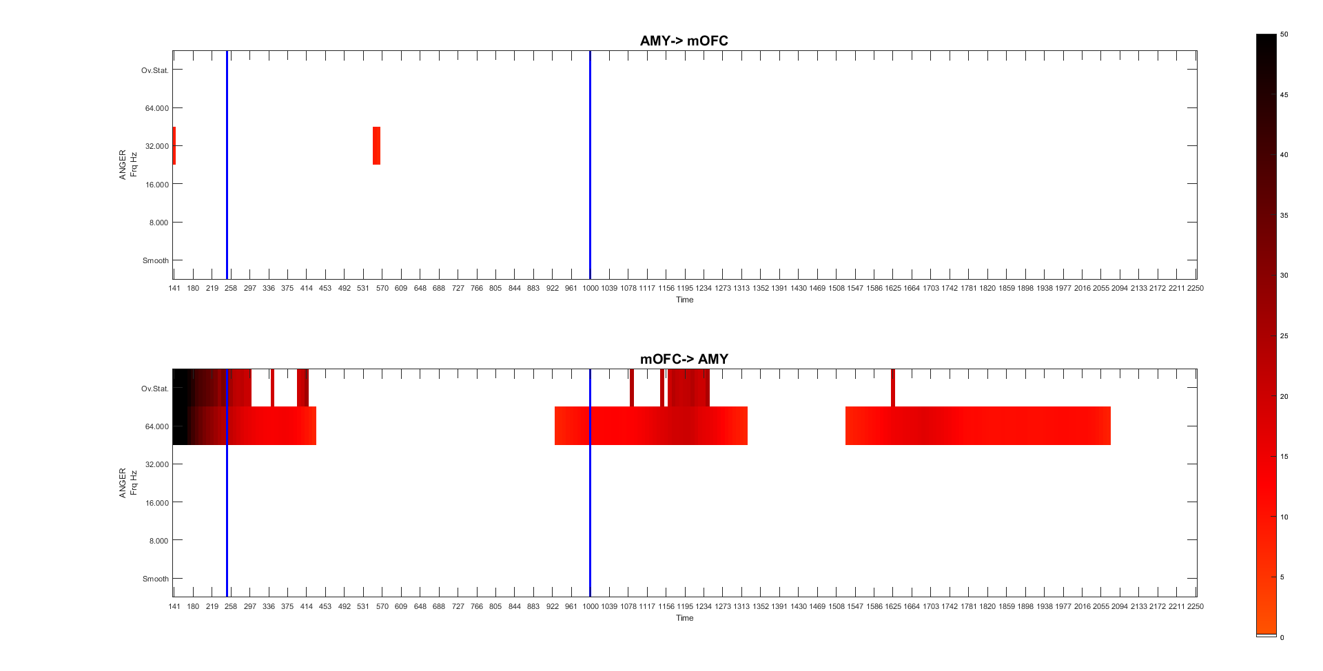
Figure 3: Results of the estimated Granger causality for the two causal links of interest AMY $\rightarrow$ mOFC and mOFC $\rightarrow$ AMY for the overall causality statistic and the scale specific causality statistics. Intensity represents the value of the individual statistic. Only the clusters assessed significant by the cluster mass test are displayed. Vertical lines represent the onset and the offset of the stimulus which occur respectively at $250$ms and $1000$ms. They are displayed for the interpretation of the results but were not provided to the model.

Figure 3 shows the results of the estimated Granger causality for the two causal links of interest AMY $\rightarrow$ mOFC and mOFC $\rightarrow$ AMY. Vertical lines represent the onset and the offset of the stimulus which occur respectively at $250$ms and $1000$ms. They are displayed for the interpretation of the results but were not provided to the model. The estimated model order for each scale plus the smooth is [5 5 3 1 1]. Only the clusters assessed significant by the cluster mass test are displayed and the colors represent the value of the individual statistic. As mentioned in Section 4, the smooth represents the frequency content of the series from the largest scale to the lowest frequency in the signal.

These results give a partial answer to the question of how AMY and mOFC regions are functionally and causally related during the exposure of auditory emotional stimuli. Actually, an initial Granger causality event from mOFC $\rightarrow$ AMY is observed in gamma range ($64$Hz) just before the stimuli onset and during stimulus exposure followed by an AMY $\rightarrow$ mOFC in beta range ($32$Hz) during this same period. At the offset of the stimuli the Granger causality is again from mOFC $\rightarrow$ AMY in gamma range ($64$Hz), this directional Granger causality is sustained during the period after the stimuli presentation. These results are compatible with a known complex cross-talk between these two brain regions during emotional stimulus exposure and the related meaning of such event for the organism. Of course such results should be extended to several patients with similar brain recordings in targeted brain regions and compared to the processing of other emotional stimuli.

8 Conclusion

We derived a time-varying Granger-causality statistic through a Bayesian nonstationary multivariate time series model with dynamic coefficients. While similar models have been proposed [9], one of the main contributions of this article is to provide an assessment of accuracy of the method, and especially an extension to the à trous Haar wavelets transform [41]. This very flexible à trous Haar procedure enables us to capture short- and long-range dependencies between signals with only few parameters to be estimated and allows us to be specific for the frequency in the assessment of causality, which is a main point of interest in the neuroscience community. The central finding of this article is that variational Bayesian estimate of time-varying VAR models enables us to achieve good (if not excellent) accuracy in terms of Granger-causality detection for normal, but also for non-normal errors and that the method performs much better than the commonly used windowing methodology in terms of Granger-causality detection accuracy. This model thus provides a very powerful tool for dynamical spectral causality analysis in a neuroscientific context.

Further points to highlight are the suitability of the model to deal with multiple trial in a fully correct way and the potential extensibility of the model to deal with more than two signals, or two sites of interest.

The choice of the sampling frequency (e.g. for EEG recordings) and the preprocessing steps commonly perform by researchers in neuroscience are two delicate issues for subsequent Granger-causality analysis, because different choices may lead to different Granger-causality results. Due to the multiscale decomposition, the MSBSS model is probably much more robust in this regard, and this would be an interesting topic for further research.

Toolbox and Appendix

An open matlab toolbox called MSGranger is available at the following url: https://www.unige.ch/fapse/mad/services/matlab/msgranger/. Single and multiple trials are implemented and both the Bayesian State Space (BSS) and the multiscale Bayesian state space (MSBSS) models can be used to obtain dynamical and frequency-specific Granger-causalities.

Appendices with all the derivations, Figures referenced in the text, as well as the cluster mass test and data analysed in Section 7 are available in the appendix.

SUPPLEMENTARY MATERIAL

Appendix A Elements of variational Bayes

The most common type of variational Bayesian methodology, known as mean-field approximation uses the Kullback–Leibler distance (KL distance) between $q(.|Z_{1}^{T})$ and $p(.|Z_{1}^{T})$ as a dissimilarity function.

A.0.1 Learning rules

By simple algebra, we will decompose the evidence of the model $p(Z_{1}^{T})$ by inserting the variational density $q$. Using the fact that $p(\varphi_{1}^{T},\Omega_{1}^{b},Z_{1}^{T})=p(\varphi_{1}^{T},\Omega_{1}^{b}|Z_{1}^{T})p(Z_{1}^{T})$, we have

$$\mathrm{KL}\big{(}q(\varphi_{1}^{T},\Omega_{1}^{b}|Z_{1}^{T})\|p(\varphi_{1}^{T},\Omega_{1}^{b}|Z_{1}^{T})\big{)}=\left<\log\frac{q(\varphi_{1}^{T},\Omega_{1}^{b}|Z_{1}^{T})}{p(\varphi_{1}^{T},\Omega_{1}^{b},Z_{1}^{T})}\right>_{q(\varphi_{1}^{T},\Omega_{1}^{b}|Z_{1}^{T})}+\log p(Z_{1}^{T}),$$ (9)

and therefore

$$\log p(Z_{1}^{T}) =\mathrm{KL}\big{(}q(\varphi_{1}^{T},\Omega_{1}^{b}|Z_{1}^{T})\|p(\varphi_{1}^{T},\Omega_{1}^{b}|Z_{1}^{T})\big{)}-\left<\log\frac{q(\varphi_{1}^{T},\Omega_{1}^{b}|Z_{1}^{T})}{p(\varphi_{1}^{T},\Omega_{1}^{b},Z_{1}^{T})}\right>_{q(\varphi_{1}^{T},\Omega_{1}^{b}|Z_{1}^{T})},$$ (10)

where $\left<.\right>$ denotes expectation and its subscript denotes the density used for this expectation. Equation (LABEL:VB_freeNRJ) is the fundamental equation of variational Bayesian methodology. By necessary positiveness of the KL distance, we have obtained a lower bound for the logarithm of the evidence

$$\log p(Z_{1}^{T}) \geq-\left<\log\frac{q(\varphi_{1}^{T},\Omega_{1}^{b}|Z_{1}^{T})}{p(\varphi_{1}^{T},\Omega_{1}^{b},Z_{1}^{T})}\right>_{q(\varphi_{1}^{T},\Omega_{1}^{b}|Z_{1}^{T})}:=\text{F}\big{(}q(\varphi_{1}^{T},\Omega_{1}^{b}|Z_{1}^{T})\big{)},$$ (11)

where $\text{F}\big{(}q(\varphi_{1}^{T},\Omega_{1}^{b}|Z_{1}^{T})\big{)}$ is called the negative free energy. By minimization of the KL distance between $q$ and $p$, we maximize $\text{F}\big{(}q(\varphi_{1}^{T},\Omega_{1}^{b}|Z_{1}^{T})\big{)}$. Furthermore, since the KL distance is equal to zero if and only if the two densities $q(\varphi_{1}^{T},\Omega_{1}^{b}|Z_{1}^{T})$ and $p(\varphi_{1}^{T},\Omega_{1}^{b}|Z_{1}^{T})$ are identical, the functional quantity $\text{F}\Big{(}q(\varphi_{1}^{T},\Omega_{1}^{b}|Z_{1}^{T})\Big{)}$ equals the model evidence if and only if $q(\varphi_{1}^{T},\Omega_{1}^{b}|Z_{1}^{T})$ equals the true target posterior $p(\varphi_{1}^{T},\Omega_{1}^{b}|Z_{1}^{T})$. The aim is thus to find a density $q(\varphi_{1}^{T},\Omega_{1}^{b}|Z_{1}^{T})$ for which the integrals in $\text{F}\Big{(}q(\varphi_{1}^{T},\Omega_{1}^{b}|Z_{1}^{T})\Big{)}$ are tractable and which is close to $p(\varphi_{1}^{T},\Omega_{1}^{b}|Z_{1}^{T})$.

A.0.2 Mean-field approximation

The choice underlying the variational Bayesian methodology, known as mean-field approximation in physics, is to allow the approximating density $q(\varphi_{1}^{T},\Omega_{1}^{b}|Z_{1}^{T})$ to factorize over groups of parameters [see 19, for a comparison between Laplace and variational Bayesian assumptions]. We will suppose here that the approximating density factorizes as

$$q(\varphi_{1}^{T},\Omega_{1}^{b}|Z_{1}^{T})=q(\varphi_{1}^{T}|Z_{1}^{T})\prod_{j=1}^{b}q(\Omega_{j}|Z_{1}^{T}),$$ (12)

and the lower bound for the model evidence can be rewritten based on this factorization as

$$\text{F}\Big{(}q(\varphi_{1}^{T}|Z_{1}^{T}),q(\Omega_{1}|Z_{1}^{T}),\dots,q(\Omega_{b}|Z_{1}^{T})\Big{)}.$$ (13)

Depending on the model at hand, mean field approximation may have minor to major impacts on the resulting inference. For example, if $p(\varphi_{1}^{T},\Omega_{1}^{b}|Z_{1}^{T})$ is such that $\varphi_{1}^{T}$ and $\Omega_{1}^{b}$ have a high degree of dependence, then the restriction $q(\varphi_{1}^{T},\Omega_{1}^{b}|Z_{1}^{T})$ = $q(\varphi_{1}^{T}|Z_{1}^{T})$ $q(\Omega_{1}^{b}|Z_{1}^{T})$ will lead to serious degradation in the resulting inference [38, 49, 6]. The factorization in equation (12) is obviously not unique. For instance, some authors factorize also $\varphi_{1}^{T}$ into $[\varphi_{1},\dots,\varphi_{T}]$ [51].

A.0.3 Variational EM algorithm

With the use of the calculus of variations (hence the name variational Bayes), it can be shown that under assumption (12), the variational distributions $q^{*}(\varphi_{1}^{T}|Z_{1}^{T})$ and $q^{*}(\Omega_{j}|Z_{1}^{T})$, that maximize the functional $\text{F}\Big{(}q(\varphi_{1}^{T}|Z_{1}^{T}),$ $q(\Omega_{1}|Z_{1}^{T}),\dots,q(\Omega_{b}|Z_{1}^{T})\Big{)}$, can be expressed and therefore maximized in an iterative way [6, 18]. First,

$$q^{*}(\varphi_{1}^{T}|Z_{1}^{T})^{(l+1)}\propto\exp\left<\log p(\varphi_{1}^{T}|\Omega_{1}^{k},Z_{1}^{T})\right>_{q(\Omega_{1}^{b}|Z_{1}^{T})}^{(l)},$$ (14)

where superscript $(l)$ denotes the iteration number. The other steps for $m=1,\dots,b$ are

$$q^{*}(\Omega_{m}|Z_{1}^{T})^{(l+1)}\propto\exp\left<\log p(\Omega_{1}^{k}|\varphi_{1}^{T},Z_{1}^{T})\right>_{-\Omega_{m}}^{(l)},$$ (15)

where $\left<.\right>_{-\Omega_{m}}^{(l)}$ is the expectation over all the distributions at iteration ${l}$ except $q(\Omega_{m}|Z_{1}^{T})^{(l)}$. See Beal [6] and Ostwald et al. [39] for all proofs.

The distributions $\exp\left<\log p(\varphi_{1}^{T}|\Omega_{1}^{k},Z_{1}^{T})\right>_{-\varphi_{1}^{T}}^{(l)}$ and $\exp\left<\log p(\Omega_{1}^{k}|\varphi_{1}^{T},Z_{1}^{T})\right>_{-\Omega_{m}}^{(l)}$ are known as full conditionals in the MCMC literature. The mutual dependence of the optimal variational posterior densities in equations (14) and (15) suggest a similarity with Gibbs sampling [8] which involves successive draws from the full conditionals. Mean field approximation indeed leads to tractable solutions in situations where Gibbs sampling is also applicable.

Thus, if we set $q(\varphi_{1}^{T}|Z_{1}^{T})$ equal to $q^{*}(\varphi_{1}^{T}|Z_{1}^{T})$ and $q(\Omega_{m}|Z_{1}^{T})$ equal to $q^{*}(\Omega_{m}|Z_{1}^{T})$, we have maximized the lower bound for the model evidence F under the (12) constraint.

The form of equations (14) and (15) define a circular dependence which explains the use of an iterative algorithm whose convergence can be assessed by monitoring the relative increase of F. This iterative algorithm is known as the variational Bayesian expectation-maximisation algorithm [6]. The result is that the formulas for the sufficient statistics of each unknown distribution $q^{*}(.|Z_{1}^{T})$ can be expressed as a series of equations with mutual dependencies. As discussed in Beal [6] and Cassidy [9], this variational Bayesian EM algorithm reduces to the ordinary frequentist EM algorithm for maximum likelihood estimate [16] if the parameter priors are flat.

A.0.4 Directed acyclic graphs and Markov blanket theory

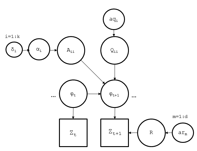
Figure 4: DAG representation of the full model given in Section 3.

The model proposed in Section 2 can be viewed as a hierarchical Bayesian model and hence can be represented as a probabilistic directed acyclic graph (DAG). This DAG representation is very useful for visualising the relationships between hidden variables ($\varphi_{1}^{T}$), parameters ($\Omega_{1}^{b}$) and observations ($Z_{1}^{T}$), each of them being represented as nodes. Typically, square nodes indicate observed variables, round nodes indicate latent random variables and arrows act for conditional dependence. Figure 4 contains the DAG for the full model considered in the present article. Moreover for models having such a structure, the variational Bayesian algorithm benefits from a graphical-related concept hailing from machine learning theory, known as variational message passing [54]. More specifically, the benefits for variational Bayesian models are directly related to the concept of Markov blanket that we will first define.

Definition A.1

The Markov blanket of a node $x_{i}$ in a DAG ($mb(x_{i})$) is defined as the set of its parents, $pa(x_{i})$, children, $ch(x_{i})$, and co-parents, $cop(x_{i})$. Two nodes are defined co-parents if they have at least one child node in common [54].

The point of particular interest for variational Bayesian theory is that the variational sequential update equation for a node $\Omega_{m}$ only depends on expectations over variables in its Markov blanket. It directly follows that equation (15) can be rewritten as

$$q^{*}(\Omega_{m}|Z_{1}^{T})^{(l+1)}\propto\exp\left<\log p(\Omega_{1}^{b}|mb(\Omega_{m}),Z_{1}^{T})\right>_{mb(\Omega_{m})}^{(l)}.$$ (16)

Fox and Roberts [18] show that equation (16) can be rewritten in an even simpler form as

$$\ln q^{*}(\Omega_{m}|Z_{1}^{T})^{(l+1)}= \left<\ln p(\Omega_{m}|pa(\Omega_{m}),Z_{1}^{T})\right>_{pa(\Omega_{m})}^{(l)}+$$ (17)

$$\sum\limits_{ch_{i}\in ch}\left<\ln p(ch_{i}|\Omega_{m},cop(\Omega_{m});ch_{i},Z_{1}^{T})\right>_{ch_{i},cop(\Omega_{m};ch_{i})}^{(l)}+\text{ct}.$$

Equation (16) is much simpler than equation (15). Similar simplifications can be obtained for equation (14).

A.0.5 Conjugate exponential

The optimal form for $q^{*}(\varphi_{1}^{T}|Z_{1}^{T})$ and $q^{*}(\Omega_{1}^{b}|Z_{1}^{T})$ of course depends on the choice of the prior distributions $p(\varphi_{1}^{T})$ and $p(\Omega_{m})$. The analytical form of $q^{*}(.|Z_{1}^{T})$ can be assessed via the following theorem [6].

Theorem A.2

For models with observed variables $Z_{1}^{T}$, hidden variables $\varphi_{1}^{T}$ and parameters $\Omega_{1}^{b}$, the mean field variational Bayesian approximation has the following characteristic: if the complete-data likelihood $p(\varphi_{1}^{T},Z_{1}^{T}|\Omega_{1}^{b})$ is part of the exponential family (in its “natural form”, meaning parametrized by its natural parameter), and if the hidden and parameter prior distributions $p(\varphi_{1}^{T})$ and $p(\Omega_{1}^{b})$ are conjugate to this complete-data likelihood, then the corresponding variational approximate posterior distributions that maximize F, $q^{*}(\varphi_{1}^{T}|Z_{1}^{T})$ and $q^{*}(\Omega_{1}^{b}|Z_{1}^{T})$, are of the same distributional form as the prior distributions $p(\varphi_{1}^{T})$ and $p(\Omega_{1}^{b})$ respectively.

As stated in Beal [6, p. 160], with suitable priors, the state space model with unknown parameters is in the conjugate-exponential family, but the “natural form” parametrization required by Theorem A.2 presents a parameter-to-natural parameter mapping that is non-invertible. We can however use the fact that all the nodes of the model defined in Section 2 are conditionally conjugate, implying that the optimal variational approximate posterior distributions $q^{*}(\varphi_{1}^{T}|Z_{1}^{T})$ and $q^{*}(\Omega_{1}^{b}|Z_{1}^{T})$ will be of the same distributional form as, respectively, the prior distributions $p(\varphi_{1}^{T})$ and $p(\Omega_{1}^{b})$ (a node is said to be conditionally conjugate when its conditional distribution given its Markov blanket (see Definition A.1) is in the same family as its conditional distribution given its parents).

Theorem A.2 moreover ensures that the analytical form of the variational distributions $q^{*}(\Omega_{m}|Z_{1}^{T})^{(l)}$ and $q^{*}(\varphi_{1}^{T}|Z_{1}^{T})^{(l)}$ does not change during iterations. Since this property does not hold for general equations (14) and (15), variational posterior distributions become quickly unmanageable outside the conjugate exponential framework. All proofs of Theorem A.2 and related properties can be found in Beal [6].

A.1 The variational evidence lower bound

In Bayesian analysis, the evidence (or marginal likelihood) provides a natural criterion for model selection by comparing the evidences obtained for the models to be compared. Well-known criteria based on evidence comparison are the Bayesian Information Criterion (BIC) and the Bayes Factor.

As observed in equation (11), the variational Bayesian methodology has the advantage of providing a quantity, the free energy, that is a lower bound for the marginal likelihood of the model and that can be computed efficiently. This leads to a natural criterion for model order selection, which is crucial to estimating our time-varying VAR model, where we have many more variables to estimate than available observations. We can therefore perform model selection by comparing the free-energy quantities computed for each model order $m_{p}$ and select the model that exhibits the highest $\text{F}_{m_{p}}$. This latter comparison supposes that we have placed uniform priors over each model structure $m_{p}$, thereby considering them as equiprobable.

Recalling equations (11), (12) and letting $m_{p}$ be the model estimated for a specific order $p$, the free-energy quantity can be re-expressed as

$$\text{F}_{m_{p}} =\left<\log\frac{p(\varphi_{1}^{T},Z_{1}^{T},\Omega_{1}^{b}|m_{p})}{q(\varphi_{1}^{T},Z_{1}^{T}|m_{p})}\right>_{q(\varphi_{1}^{T},\Omega_{1}^{b}|m_{p})}-\left<\log\frac{q(\Omega_{1}^{b}|Z_{1}^{T},m_{p})}{p(\Omega_{1}^{b}|m_{p})}\right>_{q(\Omega_{1}^{b}|Z_{1}^{T},m_{p})},$$ (18)

where the first right-hand side term is the average log-likelihood over the entire set of parameters and hidden states $[\Omega_{1}^{b};\varphi_{1}^{T}]$ that therefore acts as an accuracy term, and the second right-hand side term is the Kullback–Leibler distance between the prior and the variational posterior distributions for the entire set of parameters $\Omega_{1}^{b}$. Since the Kullback–Leibler distance increases with the number of parameters, this second term acts as a penalty.

The choice of $\text{F}_{m_{p}}$ (instead of $p(Z_{1}^{T})$) as a criterion for model order selection implicitly assumes that the free energy lies at the same distance to the evidence whatever the model order $p$. This seems reasonable, given that the dataset $Z_{1}^{T}$ is the same for all models. A similar procedure for model order selection can be found in Corduneanu and Bishop [14] and Roberts and Penny [42].

It has been shown that in the large sample limit, the free energy becomes equivalent to the Bayesian information criterion (BIC) [2]. This popular model order selection criterion can therefore be seen as a limiting case of the variational Bayesian framework [6, 40].

The specific analytic form of $\text{F}_{m_{p}}$ for our model is derived in Appendix B.

Appendix B Computation of the Free Energy

It is straightforward to re-express the free-energy quantity as

$$\begin{split}\mathbf{F}=&-\left<\log\frac{q(\Omega_{1}^{b}|Z_{1}^{T})}{p(\Omega_{1}^{b})}\right>_{q(\Omega_{1}^{b}|Z_{1}^{T})}-\left<\log q(\varphi_{1}^{T}|Z_{1}^{T})\right>_{q(\varphi_{1}^{T}|Z_{1}^{T})}\\ &+\left<\log p(\varphi_{1}^{T},Z_{1}^{T}|\Omega_{1}^{b},m_{p})\right>_{q(\varphi_{1}^{T},\Omega_{1}^{b}|Z_{1}^{T})},\\ \end{split}$$ (19)

where we omit the conditional dependence to the model $m_{p}$ for notational simplicity. The first term on the r.h.s. of equation (19) represents the Kullback–Leibler divergence between the prior and the variational posterior for the entire set of parameters $\Omega_{1}^{b}$, the second r.h.s. term represents the entropy of the variational posterior distribution of the hidden variables $\varphi_{1}^{T}$ and the third r.h.s. term is the average log-likelihood of the data and hidden state parameters taken over the entire set of parameters $\Omega_{1}^{b}$ and hidden state $\varphi_{1}^{T}$.

Recalling the mean-field factorization assumed in our model as well as the priors distributions set in Section 4, the free-energy quantity takes the explicit form:

$$\begin{split}\mathbf{F}=&-\left<\log\frac{q(A)}{p(A|\mathbf{\alpha)}}\right>_{q(A)}-\left<\log\frac{q(\mathbf{\alpha}|\mathbf{\delta})}{p(\mathbf{\alpha}|\mathbf{\delta}}\right>_{q(\mathbf{\alpha}|\mathbf{\delta})}-\left<\log\frac{q(\mathbf{\delta})}{p(\mathbf{\delta})}\right>_{q(\mathbf{\delta})}\\ &-\left<\log\frac{q(Q|a_{q})}{p(Q|a_{q})}\right>_{q(Q|a_{q})}-\left<\log\frac{q(a_{q})}{p(a_{q})}\right>_{q(a_{q})}\\ &\underbrace{-\left<\log\frac{q(R|\{a_{ri}\}_{i=1}^{d})}{p(R|\{a_{ri}\}_{i=1}^{d})}\right>_{q(R|\{a_{ri}\}_{i=1}^{d})}-\left<\log\frac{q(\{a_{ri}\}_{i=1}^{d})}{p(\{a_{ri}\}_{i=1}^{d})}\right>_{q(\{a_{ri}\}_{i=1}^{d})}}_{\text{term 1}}\\ &\underbrace{-\left<\log q(\varphi_{1}^{T})\right>_{q(\varphi_{1}^{T})}}_{\text{term 2}}\underbrace{+\left<\log p(\varphi_{1}^{T},Z_{1}^{T}|\Omega_{1}^{b})\right>_{q(\varphi_{1}^{T})q(\Omega_{1}^{b})}}_{\text{term 3}},\end{split}$$ (20)

where the conditional dependance of the variational posterior distributions $q(.)$ to the data $Z_{t}$ is now omitted for notational simplicity.

The KL divergences of term 1 have closed form for conjugate exponential distributions and are therefore straightforward to obtain despite their intensive computation. Let us focus on the entropy term that appears in term 2. Following [6], this can be rewriten as

term 2 $$=-\left<\log q(\varphi_{1}^{T})\right>_{q(\varphi_{1}^{T})}=-\left<-\log\Upsilon+\underbrace{\left<\log p(\varphi_{1}^{T},Z_{1}^{T}|\Omega_{1}^{b})\right>_{q(\Omega_{1}^{b})}}_{\text{term 3}}\right>_{q(\varphi_{1}^{T})}.$$ (21)

Term 3 therefore disappears in equation (20) and the quantity $\Upsilon$ becomes

$$\Upsilon =\left<\exp\left<\log p(\varphi_{1}^{T},Z_{1}^{T}|\Omega_{1}^{b})\right>_{q(\Omega_{1}^{b})}\right>_{q(\varphi_{1}^{T})}$$ (22)

$$=\underbrace{\left<\exp\left<\log p(\varphi_{1}^{T}|Z_{1}^{T},\Omega_{1}^{b})\right>_{q(\Omega_{1}^{b})}\right>_{q(\varphi_{1}^{T})}}_{=1}+\left<\exp\left<\log p(Z_{1}^{T}|\Omega_{1}^{b})\right>_{q(\Omega_{1}^{b})}\right>_{q(\varphi_{1}^{T})}.$$

Assuming now that the parameters $\Omega_{1}^{b}$ have a point mass density rather than their variational posterior distribution $q(.)$, the $\Upsilon$ quantity becomes

$$\Upsilon =\left<\exp\left<\log p(Z_{1}^{T}|\Omega_{1}^{b})\right>_{q(\Omega_{1}^{b})}\right>_{q(\varphi_{1}^{T})}=p(Z_{1}^{T}|\bar{R})=p(Z_{1})\prod_{t=2}^{T}p(Z_{t}|Z_{1}^{t-1}).$$ (23)

The quantity $\Upsilon$ can be obtained just after the forward recursion step and therefore amounts to

$$\Upsilon =p(Z_{1})\prod_{t=2}^{T}p(Z_{t}|Z_{1}^{t-1})=\prod_{t=1}^{T}\mathcal{N}_{d}(C_{t}\mu_{t}^{t-1},C_{t}\Sigma_{t}^{t-1}C_{t}^{{}^{\prime}}+R),$$ (24)

where the quantities $\mu_{t}^{t-1}$ and $\Sigma_{t}^{t-1}$ are defined in Appendix D [43].

Appendix C Mean and Fluctuation Theorem

The Mean and Fluctuation Theorem is a decomposition proved by [3]. Using our notation, based on the model and the Conditional distributions defined in Section 2 and the set of unknown parameters $\Omega_{1}^{b}$, the following decomposition of the density $\left<\log p(\varphi_{1}^{T},Z_{1}^{T}|\Omega_{1}^{b})\right>_{q(\Omega_{1}^{b}|Z_{1}^{T})}$ holds

$$\begin{split}\left<\log p(\varphi_{1}^{T},Z_{1}^{T}|\Omega_{1}^{b})\right>_{q(\Omega_{1}^{b}|Z_{1}^{T})}=&\log p(\varphi_{1}^{T},Z_{1}^{T}|\left<\Omega_{1}^{b}\right>)+F_{A,Q}+F_{C_{t},R},\quad\text{where}\\ \log p(\varphi_{1}^{T},Z_{1}^{T}|\left<\Omega_{1}^{b}\right>)\propto&\frac{1}{2}(\varphi_{1}-\mu_{1})\Sigma_{1}^{-1}(\varphi_{1}-\mu_{1})^{{}^{\prime}}\\ &-\frac{1}{2}\sum_{t=2}^{T}(\varphi_{t}-\left<A\right>\varphi_{t-1})Q^{-1}(\varphi_{t}-\left<A\right>\varphi_{t-1})^{{}^{\prime}}\\ &-\frac{1}{2}\sum\limits_{t=1}^{T}(Z_{t}-C_{t}\varphi_{t})R^{-1}(Z_{t}-C_{t}\varphi_{t})^{{}^{\prime}},\\ F_{A,Q}=&-\frac{1}{2}\sum_{t=1}^{T-1}\varphi_{t}^{{}^{\prime}}\big{(}\left<AQ^{-1}A\right>-\left<A\right>\left<Q\right>^{-1}\left<A\right>\big{)}\varphi_{t},\\ F_{C_{t},R}=&-\frac{1}{2}\sum_{t=1}^{T}\varphi_{t}^{{}^{\prime}}\big{(}\left<C_{t}R^{-1}C_{t}\right>-\left<C_{t}\right>\left<R\right>^{-1}\left<C_{t}\right>\big{)}\varphi_{t}.\end{split}$$ (25)

Note that the formulation in [3] considers the matrix $C_{t}$ as time-invariant.

Appendix D Unified Inference Theorem

For the BSS model, recall equation (14), which is a key quantity we want to evaluate

$$q^{*}(\varphi_{1}^{T})^{(t+1)}\propto\exp\left<\log p(\varphi_{1}^{T},\Omega_{1}^{b},Z_{1}^{T})\right>_{q(\Omega_{1}^{b})}^{(t)}\propto\exp\left<\log p(\varphi_{1}^{T}|\Omega_{1}^{b},Z_{1}^{T})\right>_{q(\Omega_{1}^{b})}^{(t)}.$$

In the situation where $\Omega_{1}^{b}$ are random parameters rather than fixed values, Barber and Chiappa [3] propose an elegant solution based on a suitably augmented system of equations that allows to infer $q(\varphi_{1}^{T})$ through classical state space model inference algorithms. The theorem states that the above density can be written as

$$\exp\left<\log p(\varphi_{1}^{T}|\Omega_{1}^{b},Z_{1}^{T})\right>_{q(\Omega_{1}^{b})}=p(\varphi_{1}^{T}|\widetilde{\Omega_{1}^{b}},\widetilde{Z}_{1}^{T}),$$ (26)

where the augmented elements are

$$\begin{split}\widetilde{\Omega}_{1}^{b}=\{\widetilde{A};\widetilde{Q};\widetilde{R}\},\qquad\widetilde{A}=\left<A\right>,\qquad\widetilde{Q}=\left<Q\right>,\qquad\widetilde{R}=\begin{pmatrix}\left<R\right>&0&0\\ 0&I_{k}&0\\ 0&0&I_{d}\end{pmatrix},\\ \widetilde{Z}_{t}=\begin{pmatrix}Z_{t}\\ 0_{k}\\ 0_{d}\end{pmatrix},\qquad\widetilde{C}_{t}=\begin{pmatrix}C_{t}\\ U_{A}\\ U_{C_{t}}\end{pmatrix},\qquad\end{split}$$

and where $U_{A}$ and $U_{C_{t}}$ are defined as the Cholesky decompositions of

$$\begin{split}U_{A}^{{}^{\prime}}U_{A}&=\left<AQ^{-1}A\right>-\left<A\right>\left<Q\right>^{-1}\left<A\right>,\\ U_{C_{t}}^{{}^{\prime}}U_{C_{t}}&=\left<C_{t}R^{-1}C_{t}\right>-\left<C_{t}\right>\left<R\right>^{-1}\left<C_{t}\right>.\end{split}$$

In our specific case, we have that $U_{C_{t}}^{{}^{\prime}}U_{C_{t}}=0$, due to the non-randomness of the matrix $C_{t}$, and so the unique quantity to define is $U_{A}^{{}^{\prime}}U_{A}$. In the case where $A$ and $Q$ are diagonal as defined in Section 3, we have that

$$\begin{split}U_{A}^{{}^{\prime}}U_{A}=&\left<AQ^{-1}A\right>-\left<A\right>\left<Q\right>^{-1}\left<A\right>\\ =&\begin{pmatrix}\left<A_{1,1}q_{1}^{-1}A_{1,1}\right>&0&0\\ \vdots&\ddots&\vdots\\ 0&0&\left<A_{k,k}q_{k}^{-1}A_{k,k}\right>\end{pmatrix}\\ &-\begin{pmatrix}\left<A_{1,1}\right>\left<q_{1}^{-1}\right>\left<A_{1,1}\right>&0&0\\ \vdots&\ddots&\vdots\\ 0&0&\left<A_{k,k}\right>\left<q_{k}^{-1}\right>\left<A_{k,k}\right>\end{pmatrix},\\ =&\begin{pmatrix}\left<A_{1,1}^{2}\right>\left<q_{1}^{-1}\right>&0&0\\ \vdots&\ddots&\vdots\\ 0&0&\left<A_{k,k}^{2}\right>\left<q_{k}^{-1}\right>\end{pmatrix}-\begin{pmatrix}\left<A_{1,1}\right>^{2}\left<q_{1}^{-1}\right>&0&0\\ \vdots&\ddots&\vdots\\ 0&0&\left<A_{k,k}\right>^{2}\left<q_{k}^{-1}\right>\end{pmatrix},\\ =&\begin{pmatrix}\sigma_{A_{1,1}}^{2}\left<q_{1}^{-1}\right>&0&0\\ \vdots&\ddots&\vdots\\ 0&0&\sigma_{A_{k,k}}^{2}\left<q_{k}^{-1}\right>\end{pmatrix},\end{split}$$ (27)

where $\sigma_{A_{i,i}}^{2}$ is the variational posterior variance of the $i$-th entry of the $A$ matrix defined in Section H and $\left<q_{i}^{-1}\right>$ is the variational posterior mean of the $i$-th entry of the inverse variance-covariance matrix $Q^{-1}$ defined in Section J that can be straightforwardly obtained due to the properties of the inverse-gamma and gamma distributions.

For our model, the augmented system of equations then gives

$$\begin{split}\widetilde{Z}_{t}=\begin{pmatrix}Z_{t}\\ 0_{k}\end{pmatrix},\qquad\widetilde{A}=\left<A\right>,\qquad\widetilde{Q}=\left<Q\right>,\qquad\widetilde{C}_{t}=\begin{pmatrix}C_{t}\\ U_{A}\end{pmatrix},\qquad\widetilde{R}=\begin{pmatrix}\left<R\right>&0\\ 0&I_{k}\end{pmatrix},\end{split}$$ (28)

where $U_{A}$ is defined in equation (27). Complete proofs can be found in [3] and [39].

Appendix E E-step: Computation of the Distribution of $\varphi_{1}^{T}$

As discussed in Section A, variational Bayesian algorithms lead to EM-like iterative equations for the optimal variational densities $q^{*}(.|Z_{1}^{T})$. The variational update equation form for the hidden variables $\varphi_{1}^{T}$ was state in equation (14). The derivation of equation (14) can be found in Appendix E. Due to the conjugacy condition discussed in Section A and equation the Conditional distributions stated in Section 2, the variational posterior distribution $q^{*}(\varphi_{1}^{T}|Z_{1}^{T})$ is multivariate Gaussian of dimension $k\times T$. As explained in Beal [6] and Cassidy [9], if the parameters $\Omega_{1}^{b}$ were, as they called, point estimated, equation (14) would be straightforwardly resolved with classical state space model tools.

However in our variational Bayesian scenario, parameters $\Omega_{1}^{b}$ are random variables governed by a specific variational distribution $q(.|Z_{1}^{T})$, and so $\exp\left<\log p(\varphi_{1}^{T}|\Omega_{1}^{b},Z_{1}^{T})\right>_{q(\Omega_{1}^{b}|Z_{1}^{T})}$ has to be computed for each variable with respect to its variational posterior distribution $q(\Omega_{1}^{b}|Z_{1}^{T})$, sequentially for all parameters in the set $\Omega_{1}^{b}$. As described in Beal [6] and Barber and Chiappa [3] and fully explained in Ostwald et al. [39], the simplification in equation (14) no longer holds in this random parameter scenario because

$$\exp\left<\log p(\varphi_{1}^{T}|\Omega_{1}^{b},Z_{1}^{T})\right>_{q(\Omega_{1}^{b}|Z_{1}^{T})}\neq p(\varphi_{1}^{T}|\bar{\Omega}_{1}^{b},Z_{1}^{T}).$$ (29)

The difference between the two terms in equation (29) is evaluated in Barber and Chiappa [3] and its decomposition is known as the mean and fluctuation theorem, reproduced in Appendix C. To nevertheless use standard state space model algorithms to solve $\exp\left<\log p(\varphi_{1}^{T}|\Omega_{1}^{b},Z_{1}^{T})\right>_{q(\Omega_{1}^{b}|Z_{1}^{T})}$ in the variational Bayesian framework, and therefore to capitalize on the vast literature and results that exist on the topic, Barber and Chiappa [3] prove the so-called unified inference theorem recalled in Appendix C. The idea is to reformulate $\exp\left<\log p(\varphi_{1}^{T},\Omega_{1}^{b},Z_{1}^{T})\right>_{q(\Omega_{1}^{b}|Z_{1}^{T})}$ as a standard density $\widetilde{p}(\varphi_{1}^{T},\widetilde{\Omega}_{1}^{b},\widetilde{Z}_{1}^{T})$ with known parameters $\widetilde{\Omega}_{1}^{b}$, by suitably augmenting the first equation in the system defined in Section 2. The classical KRTS smoother algorithms may then be suitably applied to the new density $\widetilde{p}(\varphi_{1}^{T},\widetilde{\Omega}_{1}^{b},\widetilde{Z}_{1}^{T})$, and allows us to derive the target quantity $\widetilde{p}(\varphi_{1}^{T}|\widetilde{\Omega}_{1}^{b},\widetilde{Z}_{1}^{T})$. This finally corresponds to $\exp\left<\log p(\varphi_{1}^{T}|\Omega_{1}^{b},Z_{1}^{T})\right>_{q(\Omega_{1}^{b}|Z_{1}^{T})}$, and by extension to $q^{*}(\varphi_{1}^{T}|Z_{1}^{T})^{(t+1)}$ by equation (14).

The optimal variational posterior distribution for the hidden state sequence $\varphi_{1}^{T}$ is therefore multivariate Gaussian at each time $t$:

$$q^{*}(\varphi_{t}|Z_{1}^{T})=\mathcal{N}_{k}(\varphi_{t}|\mu_{t},\Sigma_{t}),$$ (30)

where the sufficient statistics $\{\mu_{t};\Sigma_{t}\}_{t=1}^{T}$, as well as the cross-moments $\{\mu_{t}\mu_{t-1};\Sigma_{t,t-1}\}_{t=2}^{T}$, are obtained through the KRTS smoother recursive equations applied to the suitable augmented system of equations discussed above.

Forward recursions.

This step implements the recursive equation for $q(\varphi_{t}|Z_{1}^{t})^{(l+1)}$. Let $\mu_{t}^{t}=\mathrm{E}_{q}\{\varphi_{t}|Z_{1}^{t}\}$ , $\Sigma_{t}^{t}=\mathrm{VAR}_{q}\{\varphi_{t}|Z_{1}^{t}\}$, $\mu_{t}^{t-1}=\mathrm{E}_{q}\{\varphi_{t}|Z_{1}^{t-1}\}$ , $\Sigma_{t}^{t-1}=\mathrm{VAR}_{q}\{\varphi_{t}|Z_{1}^{t-1}\}$ and $\left<.\right>$ denotes the expectation with respect to the suitable variational distribution $q(.|Z_{1}^{T})^{(l)}$. These quantities are obtained recursively as

$$\mu_{t}^{t-1} =\left<A\right>\mu_{t-1}^{t-1},$$ (31)

$$\Sigma_{t}^{t-1} =\left<A\right>\Sigma_{t-1}^{t-1}\left<A\right>^{T}+\left<Q\right>,$$

$$\mu_{t}^{t} =\mu_{t}^{t-1}+K_{t}(Z_{t}-C_{t}\mu_{t}^{t-1}),$$

$$\Sigma_{t}^{t} =\Sigma_{t}^{t-1}-K_{t}C_{t}\Sigma_{t}^{t-1},$$

where the Kalman gain $K_{t}$ is given by

$$K_{t} =\Sigma_{t}^{t-1}C_{t}^{{}^{\prime}}(C_{t}\Sigma_{t}^{t-1}C_{t}^{{}^{\prime}}+\left<R\right>)^{-1}.$$ (32)

Backward recursions.

The backward recursions implement the recursive equations for $q(\varphi_{t}|Z_{1}^{T})^{(l+1)}$. Let now $\mu_{t}^{T}=\mathrm{E}_{q}\{\varphi_{t}|Z_{1}^{T}\}$ and $\Sigma_{t}^{T}=\mathrm{VAR}_{q}\{\varphi_{t}|Z_{1}^{T}\}$. These quantities are obtained recursively as

$$J_{t} =\Sigma_{t}^{t}\left<A\right>^{{}^{\prime}}{(\Sigma_{t+1}^{t})}^{-1},$$ (33)

$$\mu_{t}^{T} =\mu_{t}^{t}+J_{t}(\mu_{t+1}^{T}-\left<A\right>\mu_{t}^{t}),$$

$$\Sigma_{t}^{T} =\Sigma_{t}^{t}+J_{t}(\Sigma_{t}^{t}-\Sigma_{t+1}^{t})J_{t}{{}^{\prime}}.$$

We also define the cross-time quantities:

$$M_{1} =\sum\limits_{t=2}^{T}\Sigma_{t}^{T}+\mu_{t}^{T}{\mu_{t}^{T}}^{{}^{\prime}},$$ (34)

$$M_{2} =\sum\limits_{t=1}^{T-1}\Sigma_{t}^{T}+\mu_{t}^{T}{\mu_{t}^{T}}^{{}^{\prime}},$$

$$M_{3} =\sum\limits_{t=2}^{T}\Sigma_{t,t-1}^{T}+\mu_{t}^{T}{\mu_{t-1}^{T}}^{{}^{\prime}},\qquad\text{where}$$

$$\Sigma_{t,t-1}^{T} =\Sigma_{t}^{t}J_{t-1}^{T}+(\Sigma_{t+1,t}^{T}-\left<A\right>\Sigma_{t}^{t})J_{t-1}^{T}.$$

This last element represents $\text{cov}_{q}(\varphi_{t},\varphi_{t-1}|Z_{1}^{T})$.

Appendix F M-step: Computation of the Distribution of $\delta$

We will derive here the update equation for $\mathbf{\delta}$ in the case where $\{\alpha_{i}\}_{i=1}^{k}$ is different for each $\{A_{i,i}\}_{i=1}^{k}$ diagonal entry of $A$. Extension to the situation where $\delta$ is a unique parameter related to a unique variance parameter $\alpha$ is straightforward.

Recalling the prior form for $\mathbf{\delta}$ defined in Section 3 as well as equation (15), the optimal form for the variational posterior $q^{*}(\mathbf{\delta}|Z_{1}^{T})$ becomes:

$$\begin{split}\begin{aligned} \log q^{*}(\mathbf{\delta}|Z_{1}^{T})^{(l+1)}=\sum_{i=1}^{k}\log q^{*}(\delta_{i}|Z_{1}^{T})^{(l+1)}=\underbrace{\sum_{i=1}^{k}\log p(\delta_{i})}_{\text{term 1}}+\underbrace{\sum_{i=1}^{k}\left<\log p(\alpha_{i}|\delta_{i})\right>_{q(\alpha_{i})^{l}}}_{\text{term 2}}+\text{ct},\end{aligned}\end{split}$$ (35)

where throughout this Supplementary Material, ct will denote the normalization constant for the given density or log-density. Recalling equation $p(\alpha_{i}|\delta_{i})$, we have that

$$\begin{split}\begin{aligned} \text{term 1}&=\sum_{i=1}^{k}(-\kappa_{p_{i}}-1)\log\delta_{i}-\delta_{i}^{-1}\beta_{p_{i}}+\text{ct},\end{aligned}\end{split}$$ (36)

and

$$\begin{split}\begin{aligned} \text{term 2}&=\sum_{i=1}^{k}-c_{p_{i}}\log\,\delta_{i}-\delta_{i}^{-1}\left<\alpha_{i}^{-1}\right>+\text{ct}.\end{aligned}\end{split}$$ (37)

The variational posterior for each element $\{\delta_{i}\}_{i=1}^{k}$ is therefore an inverse-gamma distribution with shape and scale parameters $\{\kappa_{i};\beta_{i}\}$ defined as:

$$\begin{split}\begin{aligned} \kappa_{i}&=\kappa_{p_{i}}+c_{p_{i}},\\ \beta_{i}&=\beta_{p_{i}}+\left<\alpha_{i}^{-1}\right>.\end{aligned}\end{split}$$ (38)

Appendix G M-step: Computation of the Distribution of $\alpha$

We will derive here the update equation for $\mathbf{\alpha}$ in the situation where $A$ is diagonal. Extension to the situation where $A$ is full is straightforward.

Recalling the prior form for each $\{\alpha_{i}\}_{i=1}^{k}$ defined in Section 3 as well as equation (15), the optimal form for the variational posterior $q^{*}(\alpha_{i}|\delta_{i},Z_{1}^{T})$ becomes:

$$\begin{split}\begin{aligned} \log q^{*}(\alpha|\delta,Z_{1}^{T})^{(l+1)}=&\sum_{i=1}^{k}\log q^{*}(\alpha_{i}|\delta_{i},Z_{1}^{T})^{(l+1)}\\ =&\underbrace{\sum_{i=1}^{k}\left<\log p(\alpha_{i}|\delta_{i})\right>_{q(\delta_{i})^{(l)}}}_{\text{term 1}}+\underbrace{\sum_{i=1}^{k}\left<\log p(a_{i}|\alpha_{i})\right>_{q(a_{i})^{(l)}}}_{\text{term 2}}+\text{ct},\end{aligned}\end{split}$$ (39)

where all terms not depending on $\mathbf{\alpha}$ are put in the constant term ct. Let us consider the two terms separately. Under the prior specified for $p(\alpha_{i}|\delta_{i})$, term 1 simply equals

$$\begin{split}\begin{aligned} \text{term 1}=\sum_{i=1}^{k}(-c_{p_{i}}-1)\log\alpha_{i}-\alpha_{i}^{-1}\left<\delta_{i}^{-1}\right>+\text{ct}.\end{aligned}\end{split}$$ (40)

Recalling equation for $p(\alpha_{i}|\delta_{i})$, term 2 can be rewritten as

$$\begin{split}\begin{aligned} \text{term 2}&=-\sum\limits_{i=1}^{k}\frac{1}{2}\log\alpha_{i}-\frac{\alpha_{i}^{-1}}{2}\sum\limits_{i=1}^{k}\left<(A_{ii}-m_{A_{ii}})^{2}\right>+\text{ct}\\ &=-\sum\limits_{i=1}^{k}\frac{1}{2}\log\alpha_{i}-\frac{\alpha_{i}^{-1}}{2}\sum\limits_{i=1}^{k}(\left<A_{ii}^{2}\right>+m_{A_{ii}}^{2}-2m_{A_{ii}}\left<A_{ii}\right>)^{2}+\text{ct}\\ &=-\sum\limits_{i=1}^{k}\frac{1}{2}\log\alpha_{i}-\frac{\alpha_{i}^{-1}}{2}\sum\limits_{i=1}^{k}(\theta_{i}+(\psi_{i}\theta_{i})^{2}+m_{A_{ii}}^{2}-2m_{A_{ii}}\psi_{i}\theta_{i})+\text{ct}.\end{aligned}\end{split}$$ (41)

The whole expression for $q^{*}(\mathbf{\alpha}|\mathbf{\delta},Z_{1}^{T})^{(l+1)}$ then becomes

$$\begin{split}\begin{aligned} q^{*}(\mathbf{\alpha}|\mathbf{\delta},Z_{1}^{T})^{(l+1)}=&\sum_{i=1}^{k}\log q^{*}(\alpha_{i}|\delta_{i},Z_{1}^{T})\\ =&\sum_{i=1}^{k}(-c_{p_{i}}-1)\log\alpha_{i}-\alpha_{i}^{-1}\left<\delta_{i}^{-1}\right>-\frac{1}{2}\log\alpha_{i}\\ &-\alpha_{i}^{-1}\frac{(\theta_{i}+(\psi_{i}\theta_{i})^{2}+m_{A_{ii}}^{2}-2m_{A_{ii}}\psi_{i}\theta_{i})}{2}\big{]}+\text{ct},\end{aligned}\end{split}$$ (42)

and so the variational posterior for each element $\{\alpha_{i}\}_{i=1}^{k}$ is an inverse-gamma distribution with respectively $\{c_{i};b_{i}\}$ shape and scale parameters defined as:

$$\begin{split}\begin{aligned} c_{i}&=c_{p_{i}}+\frac{1}{2},\\ b_{i}&=\left<\delta_{i}^{-1}\right>+\frac{(\theta_{i}+(\psi_{i}\theta_{i})^{2}+m_{A_{ii}}^{2}-2m_{A_{ii}}\psi_{i}\theta_{i})}{2}.\end{aligned}\end{split}$$ (43)

Appendix H M-step: Computation of the Distribution of A

The optimal form for the variational posterior $q^{*}(A|\alpha,\delta,Z_{1}^{T})$ is:

$$\begin{split}\begin{aligned} \log q^{*}(A|\alpha,\delta,Z_{1}^{T})^{(l+1)}=&\underbrace{\left<\log p(A|\alpha)\right>_{q(\varphi_{1}^{T})^{(l)},q(Q)^{(l)},q(\alpha)^{(l)}}}_{\text{term 1}}\\ &+\underbrace{\sum\limits_{t=2}^{T}\left<\log p(\varphi_{t}|\varphi_{t-1},A,Q)\right>_{q(\varphi_{1}^{T})^{(l)},q(Q)^{(l)},q(\alpha)^{(l)}}}_{\text{term 2}}+\text{ct},\end{aligned}\end{split}$$ (44)

where all terms not depending on $A$ are stacked in the constant term ct and the conditional dependence on the data $Z_{1}^{T}$ is dropped for sake of brevity. Let us consider the two terms separately. The development of term 2 is the same whatever the form for $A$ (full, diagonal or proportional to identity). It becomes

$$\begin{split}\begin{aligned} \text{term 2}&=\sum\limits_{t=2}^{T}\left<\log p(\varphi_{t}|\varphi_{t-1},Q,\alpha)\right>_{{q(\varphi_{1}^{T})^{(l)},q(Q)^{(l)}}}+\text{ct}\\ &=\sum\limits_{t=2}^{T}\left<\underbrace{\frac{1}{2}\log|Q|}_{\longrightarrow\text{ct}}-\frac{1}{2}\mathrm{Tr}[(\varphi_{t}-A\varphi_{t-1})(\varphi_{t}-A\varphi_{t-1})^{{}^{\prime}}Q]\right>_{q(\varphi_{1}^{T})^{(l)},q(Q)^{(l)}}+\text{ct}\\ &=\sum\limits_{t=2}^{T}\left<-\frac{1}{2}\mathrm{Tr}\big{[}(\varphi_{t}\varphi_{t}^{{}^{\prime}}-2A\varphi_{t-1}\varphi_{t}^{{}^{\prime}}+A\varphi_{t-1}\varphi_{t-1}^{{}^{\prime}}A^{{}^{\prime}})Q\big{]}\right>_{q(\varphi_{1}^{T})^{(l)},q(Q)^{(l)}}+\text{ct}\\ &=-\frac{1}{2}\mathrm{Tr}\left<\big{[}\underbrace{\sum\limits_{t=2}^{T}\left<\varphi_{t}\varphi_{t}^{{}^{\prime}}\right>}_{\longrightarrow\text{ct}}-2A\underbrace{\sum\limits_{t=2}^{T}\left<\varphi_{t-1}\varphi_{t}^{{}^{\prime}}\right>}_{=M_{3}\eqref{M_123}}+A\underbrace{\sum\limits_{t=2}^{T}\left<\varphi_{t-1}\varphi_{t-1}^{{}^{\prime}}\right>}_{=M_{2}\eqref{M_123}}A^{{}^{\prime}})Q\big{]}\right>_{q(Q)^{(l)}}+\text{ct}.\end{aligned}\end{split}$$ (45)

We can now rewrite (45) in term 2 of equation (44):

$$\begin{split}\begin{aligned} \text{term 2}&=-\frac{1}{2}\left<\mathrm{Tr}\big{[}-2AM_{3}Q+AM_{2}A^{{}^{\prime}}Q\big{]}\right>_{q(Q)^{(l)}}+\text{ct}\\ &=-\frac{1}{2}\mathrm{Tr}\big{[}-2AM_{3}\left<Q\right>+AM_{2}A^{{}^{\prime}}\left<Q\right>\big{]}+\text{ct}.\end{aligned}\end{split}$$ (46)

If we suppose the matrix $A$ diagonal, as implied by the prior form $p(A|\mathbf{\alpha})$ as well as equation (15), term 1 in equation (44) is straightforward:

$$\begin{split}\begin{aligned} \text{term 1}&=\sum\limits_{i=1}^{k}\left<\log p(A_{ii}|\alpha_{i})\right>_{q(\alpha_{i})^{(l)}}&=-\frac{\left<\alpha_{i}^{-1}\right>}{2}\sum\limits_{i=1}^{k}(A_{ii}-m_{A_{ii}})^{2}+\text{ct}.\end{aligned}\end{split}$$ (47)

The full expression then gives:

$$\begin{split}\begin{aligned} \log q^{*}(A|\alpha,\delta,Z_{1}^{T})^{(l+1)}=&-\frac{1}{2}\big{[}\sum\limits_{i=1}^{k}\left<\alpha_{i}^{-1}\right>(A_{ii}-m_{A_{ii}})^{2}\\ &+\mathrm{Tr}\{-AM_{3}\left<Q\right>-M_{3}A^{{}^{\prime}}\left<Q\right>+AM_{2}A^{{}^{\prime}}\left<Q\right>\}\big{]}+\text{ct}\\ =&-\frac{1}{2}\sum\limits_{i=1}^{k}\big{[}\left<\alpha_{i}^{-1}\right>(A_{ii}^{2}+m_{A_{ii}}^{2}-2A_{ii}m_{A_{ii}})-2A_{ii}M_{3_{i,i}}\left<Q_{ii}\right>\\ &+A_{ii}M_{2_{i,i}}A_{ii}\left<Q_{ii}\right>\big{]}+\text{ct}\\ =&-\frac{1}{2}\sum\limits_{i=1}^{k}\big{[}-2A_{ii}\underbrace{(\left<\alpha_{i}^{-1}\right>m_{A_{ii}}+M_{3_{i,i}}\left<q_{i}\right>)}_{:=\psi_{i}}\\ &+A_{ii}^{2}\underbrace{(\left<Q_{ii}\right>M_{2_{i,i}}+\left<\alpha_{i}^{-1}\right>)}_{:={\theta_{i}}^{-1}}+\underbrace{\left<\alpha_{i}^{-1}\right>m_{A_{ii}}^{2}}_{\longrightarrow\text{ct}}]+\text{ct}\\ =&-\frac{1}{2}\sum\limits_{i=1}^{k}\big{[}-2A_{ii}\psi_{i}{\theta_{i}}{\theta_{i}}^{-1}+A_{ii}^{2}{\theta_{i}}^{-1}\big{]}+\text{ct}.\end{aligned}\end{split}$$ (48)

Therefore

$$\begin{split}\begin{aligned} \log q^{*}(A|\alpha,\delta,Z_{1}^{T})&=\sum\limits_{i=1}^{k}\log q^{*}(A_{ii}|\alpha,\delta,Z_{1}^{T}),\\ \text{with}\qquad&q^{*}(A_{ii}|Z_{1}^{T})=\mathcal{N}_{1}(A_{ii}|\psi_{i}{\theta_{i}},{\theta_{i}}),\\ \text{where}\qquad&\theta_{i}=(\left<Q_{ii}\right>M_{2_{i,i}}+\left<\alpha_{i}^{-1}\right>)^{-1}\qquad\text{and}\\ \qquad&\psi_{i}=\left<\alpha_{i}^{-1}\right>m_{a}+M_{3_{i,i}}\left<Q_{ii}\right>.\end{aligned}\end{split}$$ (49)

Appendix I M-step: Computation of the Distribution of $a_{q}$

We will derive here the update equation for $a_{q}$ in the situation where the parameter $Q_{ii}$ is unique. Extension to the situation where $\{a_{q_{i}}\}_{i=1}^{k}$ is related to different $\{Q_{ii}\}_{i=1}^{k}$ is straightforward. Recalling the prior form for $a_{q}$ in Section 2 as well as equation (15), the optimal form for the variational posterior $q^{*}(a_{q}|Z_{1}^{T})$ becomes:

$$\begin{split}\begin{aligned} \log q^{*}(a_{q}|Z_{1}^{T})^{(l+1)}=\underbrace{\log p(a_{q})}_{\text{term 1}}+\underbrace{\left<\log p(Q_{ii}|a_{q})\right>_{q(Q_{ii})^{(l+1)}}}_{\text{term 2}}+\text{ct}.\end{aligned}\end{split}$$ (50)

Recalling the equation for $p(\alpha_{i}|\delta_{i})$, we have that

$$\begin{split}\begin{aligned} \text{term 1}&=(-a_{qp}-1)\log\,a_{q}-a_{q}^{-1}b_{qp}+\text{ct}\end{aligned}\end{split}$$ (51)

and

$$\begin{split}\begin{aligned} \text{term 2}&=-n_{p}\log a_{q}-a_{q}^{-1}\left<q^{-1}\right>+\text{ct}.\end{aligned}\end{split}$$ (52)

The variational posterior $\log q^{*}(a_{q}|Z_{1}^{T})$ is therefore an inverse-gamma distribution with shape and scale parameters $\{a_{qq};b_{qq}\}$

$$\begin{split}\begin{aligned} a_{qq}&=a_{qp}+n_{p},\\ b_{qq}&=b_{qp}+\left<q^{-1}\right>.\end{aligned}\end{split}$$ (53)

Appendix J M-step: Computation of the Distribution of $Q$

If the matrix $Q$ is proportional to identity, i.e. with only one element $Q_{ii}$, the optimal variational form for the posterior $q^{*}(Q|a_{q})$ becomes:

$$\log q^{*}(Q|a_{q})^{(l+1)}=\underbrace{\log p(Q_{ii}|a_{q})}_{\text{term 1}}+\underbrace{\sum\limits_{t=2}^{T}\left<\log p(\varphi_{t}|A\varphi_{t-1})\right>_{q(A)^{(l)},q(\varphi_{1}^{T})^{(l)}}}_{\text{term 2}}+\text{ct},$$ (54)

where all terms not depending on $Q$ are included in the constant term. Recalling the equation of $p(Q_{ii}|a_{q})$, we have that

$$\begin{split}\begin{aligned} \text{term 1}=(-n_{p}-1)\log Q_{ii}-Q_{ii}^{-1}\left<a_{q}^{-1}\right>+\text{ct},\end{aligned}\end{split}$$ (55)

and

$$\begin{split}\begin{aligned} \text{term 2}=&-\frac{T-1}{2}\log|Q|-\frac{1}{2}\sum\limits_{t=2}^{T}\left<\mathrm{Tr}\big{[}(\varphi_{t}-A\varphi_{t-1})(\varphi_{t}-A\varphi_{t-1})^{{}^{\prime}}Q^{-1}\big{]}\right>_{q(\varphi_{t},\varphi_{t-1})^{(l)},q(A)^{(l)}}\\ &+\text{ct}\\ =&-\frac{T-1}{2}\log|Q|\\ &-\frac{1}{2}\left<\mathrm{Tr}\big{[}\sum\limits_{t=2}^{T}\varphi_{t}\varphi_{t}^{{}^{\prime}}Q^{-1}-2\sum\limits_{t=2}^{T}\varphi_{t}\varphi_{t-1}^{{}^{\prime}}A^{{}^{\prime}}Q^{-1}+A\sum\limits_{t=2}^{T}\varphi_{t-1}\varphi_{t-1}^{{}^{\prime}}A^{{}^{\prime}}Q^{-1}\big{]}\right>_{q(\varphi_{t},\varphi_{t-1})^{(l)},q(A)^{(l)}}\\ &+\text{ct}\\ =&-\frac{T-1}{2}\log|Q|\\ &-\frac{1}{2}\left<\mathrm{Tr}\big{[}\left<\sum\limits_{t=2}^{T}\varphi_{t}\varphi_{t}^{{}^{\prime}}\right>Q^{-1}-2\left<\sum\limits_{t=2}^{T}\varphi_{t}\varphi_{t-1}^{{}^{\prime}}\right>A^{{}^{\prime}}Q^{-1}+A\left<\sum\limits_{t=2}^{T}\varphi_{t-1}\varphi_{t-1}^{{}^{\prime}}\right>A^{{}^{\prime}}Q^{-1}\big{]}\right>_{q(A)^{(l)}}\\ &+\text{ct}\\ =&-k\frac{T-1}{2}\log q-\frac{1}{2}\sum\limits_{i=1}^{k}\big{[}M_{1_{i,i}}-2M_{3_{i,i}}\left<a_{i}\right>+M_{2_{i,i}}\left<a_{i}^{2}\right>\big{]}Q_{ii}^{-1}+\text{ct}\\ =&-k\frac{T-1}{2}\log Q_{ii}-\frac{1}{2}\underbrace{\sum\limits_{i=1}^{k}\big{[}M_{1_{i,i}}-2M_{3_{i,i}}\psi_{i}\theta_{i}+M_{2_{i,i}}[(\psi_{i}\theta_{i})^{2}+\theta_{i}^{2}]\big{]}}_{:=\Gamma}Q_{ii}^{-1}+\text{ct}.\end{aligned}\end{split}$$ (56)

The whole expression for $q^{*}(Q_{ii}|a_{q})$ can the be rewritten as

$$\begin{split}\begin{aligned} \log q^{*}(Q_{ii}|a_{q})=(-n_{p}-1)\log Q_{ii}-Q_{ii}^{-1}\left<a_{q}^{-1}\right>-k\frac{T-1}{2}\log Q_{ii}-Q_{ii}^{-1}\frac{\Gamma}{2}+\text{ct}.\\ \end{aligned}\end{split}$$ (57)

The variational posterior distribution $q^{*}(Q_{ii}|a_{q})$ is therefore gamma with shape and scale parameters

$$\begin{split}n&=n_{p}+k\frac{T-1}{2},\\ d&=\left<a_{q}^{-1}\right>+\frac{\Gamma}{2},\end{split}$$ (58)

where $\Gamma=\sum\limits_{i=1}^{k}\big{[}M_{1_{i,i}}-2M_{3_{i,i}}\psi_{i}\theta_{i}+M_{2_{i,i}}[(\psi_{i}\theta_{i})^{2}+\theta_{i}^{2}]\big{]}$ and $\{\theta_{i};\psi_{i}\}$ are defined in equation (49).

Appendix K M-step: Computation of the Distribution of $a_{r}$

We will derive here the update equation for the parameters $\{a_{r_{i}}\}_{i=1}^{d}$. Recalling the prior form for $\{a_{r_{i}}\}_{i=1}^{d}$ defined in Section 3 and equation (15), the optimal form for the variational posterior $q^{*}(\{a_{r_{i}}\}_{i=1}^{d})$ becomes:

$$\begin{split}\begin{aligned} \log q^{*}(\{a_{r_{i}}\}_{i=1}^{d})^{(l+1)}=\underbrace{\log p(\{a_{r_{i}}\}_{i=1}^{d})}_{\text{term 1}}+\underbrace{\left<\log p(R|\{a_{r_{i}}\}_{i=1}^{d})\right>_{q(R)^{(l)}}}_{\text{term 2}}+\text{ct}.\end{aligned}\end{split}$$ (59)

Recalling equation for $p(R|a_{r_{1}},\dots,a_{r_{d}})$, we have that

$$\begin{split}\begin{aligned} \text{term 1}&=\sum_{i=1}^{d}(-a_{pr}-1)\log a_{r_{i}}-\sum_{i=1}^{d}a_{r_{i}}^{-1}b_{pr}+\text{ct},\end{aligned}\end{split}$$ (60)

and

$$\begin{split}\begin{aligned} \text{term 2}&=\frac{r_{p}}{2}\log|B_{p}|-\frac{1}{2}\mathrm{Tr}[B_{p}\left<R^{-1}\right>]+\text{ct},\qquad\text{where}\quad B_{p}=2\nu\,\text{diag}[\frac{1}{a_{r_{1}}}...\frac{1}{a_{r_{d}}}].\end{aligned}\end{split}$$ (61)

We therefore have

$$\begin{split}\begin{aligned} \text{term 2}&=\frac{r_{p}}{2}\log|2\nu\,\text{diag}[\frac{1}{a_{r_{1}}}...\frac{1}{a_{r_{d}}}]|-\frac{1}{2}\mathrm{Tr}\,[2\nu\,\text{diag}[\frac{1}{a_{r_{1}}}...\frac{1}{a_{r_{d}}}]\left<R^{-1}\right>\,]+\text{ct}\\ &=-\frac{r_{p}}{2}\sum_{i=1}^{d}\log a_{r_{i}}-\nu\sum_{i=1}^{d}a_{r_{i}}^{-1}\left<R^{-1}_{\{i,i\}}\right>+\text{ct}.\end{aligned}\end{split}$$ (62)

And then regrouping term 1 and term 2 yield to the inverse-gamma distribution for the variational posterior $\log q^{*}(a_{q}|Z_{1}^{T})$ with shape and scale parameters $\{a_{qr};b_{qr}\}$ defined as

$$\begin{split}\begin{aligned} a_{qr}&=a_{pr}+\frac{r_{p}}{2},\\ b_{qr}&=b_{pr}+\nu\left<R^{-1}_{\{i,i\}}\right>.\end{aligned}\end{split}$$ (63)

Appendix L M-step: Computation of the Distribution of $R$

Recalling the prior form for $R$, $p(R|a_{r_{1}},\dots,a_{r_{d}})$, and equation (15), the optimal form for the variational posterior $q^{*}(R|\{a_{r_{i}}\}_{i=1}^{d},Z_{1}^{T})$ is

$$\begin{split}\begin{aligned} \log q^{*}(R|\{a_{r_{i}}\}_{i=1}^{d})^{(l+1)}=&\underbrace{\left<\log p(R|\{a_{r_{i}}\}_{i=1}^{d})\right>_{q(a_{r})}}_{\text{term 1}}+\underbrace{\sum\limits_{t=1}^{T}\left<\log p(Z_{t}|C_{t}\varphi_{t})\right>_{q(\varphi_{1}^{T})^{(l)}}}_{\text{term 2}}+\text{ct},\end{aligned}\end{split}$$ (64)

where all terms not depending on $R$ are included in the constant term ct. Let us consider first the term 1. As the prior for $R$ defined in Section 3 is inverse-Wishart, term 1 becomes

$$\begin{split}\begin{aligned} \text{term 1}=&-\frac{r_{p}+d+1}{2}\log|R|-\frac{1}{2}\rm{Tr}(\left<B_{p}\right>R^{-1})+\text{ct}\\ =&-\frac{r_{p}+d+1}{2}\log|R|-\frac{1}{2}\rm{Tr}(2\nu\,\text{diag}[\frac{1}{\left<a_{r_{1}}\right>}...\frac{1}{\left<a_{r_{d}}\right>}]R^{-1})+\text{ct},\end{aligned}\end{split}$$ (65)

Let us now consider term 2:

$$\begin{split}\begin{aligned} \text{term 2}&=\sum\limits_{t=1}^{T}\left<\log p(Z_{t}|C_{t}\varphi_{t})\right>_{q(\varphi_{1}^{T})^{(l)}}+\text{ct}\\ &=-\frac{T}{2}\log|R|-\frac{1}{2}\sum\limits_{t=1}^{T}\mathrm{Tr}\big{[}\left<(Z_{t}-C_{t}\varphi_{t}){(Z_{t}-C_{t}\varphi_{t})}^{{}^{\prime}}\right>R^{-1}\big{]}+\text{ct}\\ &=-\frac{T}{2}\log|R|-\frac{1}{2}\sum\limits_{t=1}^{T}\mathrm{Tr}\big{[}\left<(Z_{t}Z_{t}^{{}^{\prime}}-2C_{t}\varphi_{t}Z_{t}^{{}^{\prime}}+C_{t}Z_{t}Z_{t}^{{}^{\prime}}C_{t}^{{}^{\prime}})\right>R^{-1}\big{]}+\text{ct}\\ &=-\frac{T}{2}\log|R|-\frac{1}{2}\mathrm{Tr}\sum\limits_{t=1}^{T}[(Z_{t}-C_{t}\mu_{t}){(Z_{t}-C_{t}\mu_{t})}^{{}^{\prime}}+C_{t}\Sigma_{t}C_{t}^{{}^{\prime}}]R^{-1}+\text{ct}.\\ \end{aligned}\end{split}$$ (66)

Assembling terms 1 and 2 in equations (65) and (66) yields to

$$\begin{split}\log q^{*}(R|\{a_{r_{i}}\}_{i=1}^{d},Z_{1}^{T})^{(l+1)}=&-\frac{r_{p}+d+1}{2}\log|R|-\frac{1}{2}\rm{Tr}(\left<B_{p}\right>R^{-1})-{\frac{T}{2}}\log|R|\\ &-\frac{1}{2}\mathrm{Tr}\underbrace{\sum\limits_{t=1}^{T}[(Z_{t}-C_{t}\mu_{t}){(Z_{t}-C_{t}\mu_{t})}^{{}^{\prime}}+C_{t}\Sigma_{t}C_{t}^{{}^{\prime}}]}_{:=B}R^{-1}+\text{ct},\end{split}$$ (67)

and then

$$\begin{split}\begin{aligned} \log q^{*}(R|\{a_{r_{i}}\}_{i=1}^{d},Z_{1}^{T})=\mathcal{IW}_{d}(R|r_{p}+T,\left<B_{p}\right>+B).\end{aligned}\end{split}$$ (68)

Appendix M Multiple trials

The model can be modified to deal with $N$ conditionally independent sequences $\{{Z_{1}^{T}}_{(j)}\}_{j=1}^{N}$ which are supposed to have the same hidden state. This reflects the case that arises during an event-related experimental paradigm, where many trials on the same condition are measured.

In Beal [6] and Cassidy [9], this extension is solved by first estimating the necessary sufficient statistics for each sequence independently in the E-step, and then by averaging these statistics to get only one set of sufficient statistics, which is representative of the entire set of independent sequences before performing the M-step. However this approach does not take into account the complex dependence of the variational posterior $q(\varphi_{1}^{T}|\{{Z_{1}^{T}}_{(j)}\}_{j=1}^{N})$ on the whole dataset $\{{Z_{1}^{T}}_{(j)}\}_{j=1}^{N}$. We can however write and solve the full evidence of all the data if we rewrite

$$\left\{\begin{aligned} \varphi_{t+1}=A\varphi_{t}+w_{t}\qquad&w_{t}\sim{\mathcal{N}_{k}(0,Q)}\\ \mathbf{Z}_{t}=\mathbf{C}_{t}\varphi_{t}+v_{t}\qquad&v_{t}\sim{\mathcal{N}_{d}(0,\mathbf{R})}\\ \end{aligned}\right.\quad\text{where}\begin{cases}\varphi_{t}=&\operatorname{vec}{[\vartheta_{1(t)},\vartheta_{2(t)},..,\vartheta_{p(t)}]}^{\prime},\\ \mathbf{Z}_{t}=&(Y_{t(1)}\ldots Y_{t(N)}X_{t(1)}\ldots X_{t(N)})^{{}^{\prime}}\\ \mathbf{C}_{t}\varphi_{t}=&\sum\limits_{j=1}^{p}\vartheta_{j(t)}(Y_{t-j(1)}\ldots Y_{t-j(N)}\\ &X_{t-j(1)}\ldots X_{t-j(N)})^{{}^{\prime}},\\ \mathbf{R}=&\text{diag}(R_{1}\ldots R_{N})^{{}^{\prime}},\end{cases}$$ (69)

where $\mathbf{R}$ is block diagonal of dimensions $d^{2}N\times d^{2}N$ with each diagonal element $R_{j}$ being identically distributed. The state equation remains the same as in model defined in Section 2. We can observe in model (69) that the time-varying parameter vectors $\{\varphi_{t}\}_{t=1}^{T}$ are unique, taking into account the whole dataset $\{{Z_{1}^{T}}_{(j)}\}_{j=1}^{N}$. The evidence of the complete model can be rewritten as

$$\begin{split}p(\{{Z_{1}^{T}}_{(j)}\}_{j=1}^{N},\varphi_{1}^{T},\Omega_{1}^{b})=&p({Z_{1}^{T}}_{(j)}\}_{j=1}^{N},\varphi_{1}^{T},\{A_{ii}\}_{i=1}^{k}\{\alpha_{i}\}_{i=1}^{k},\{\delta_{i}\}_{i=1}^{k},Q_{i,i},a_{q},\mathbf{R},\{a_{r_{i}}\}_{i=1}^{d})\\ =&\prod_{j=1}^{N}\prod_{i=1}^{T}p(Z_{t}(j)|C_{t}(j),\varphi_{t},R_{j})p(\varphi_{1})\prod_{i=2}^{T}p(\varphi_{t}|A,\varphi_{t-1},Q)\prod_{i=1}^{k}p(A_{ii}|\alpha_{i})\\ &\times\prod_{i=1}^{k}p(\alpha_{i}|\delta_{i})\prod_{i=1}^{k}p(\delta_{i})p(Q_{i,i}|a_{q})p(a_{q})p(R_{j}|\{a_{r_{i}}\}_{i=1}^{d})\prod_{i=1}^{d}p(a_{r_{i}}).\end{split}$$ (70)

All the computations done so far can easily be adapted to this new setting. The variational posterior distributions relative to model (69) are now conditional on the whole dataset $\{{Z_{1}^{T}}_{(j)}\}_{j=1}^{N}$. A detailed derivation of the model and related variational posterior distributions with multiple trials can be founded in Section M.

In the DAG depicted in Figure 4, we can see that conditional dependence on the observed variables $Z$ is present only for nodes $\{\varphi_{1}^{T};Z_{1}^{T};\mathbf{R};a_{r}\}$. For the hidden variables, the variational E-step KRTS algorithm can be run on the whole state space system (69) and the resulting variational posterior density will therefore be conditional on the whole dataset $q(\varphi_{1}^{T}|\{{Z_{1}^{T}}_{(j)}\}_{j=1}^{N})$. In Appendix E, the update equations remain the same, except for the Kalman gain in equation (32) which becomes

$$K_{t}=\Sigma_{t}^{t-1}C_{t}^{{}^{\prime}}(C_{t}\Sigma_{t}^{t-1}C_{t}^{{}^{\prime}}+\left<\mathbf{R}\right>)^{-1}.$$ (71)

Looking at the update equations for the $a_{r}$ parameter in Appendix K, we see that for multiple sequences equation (59) becomes

$$\begin{split}\begin{aligned} \log q^{*}(\{a_{r_{i}}\}_{i=1}^{d})^{(l+1)}=\underbrace{\log p(\{a_{r_{i}}\}_{i=1}^{d})}_{\text{term 1}}+\underbrace{\sum\limits_{j=1}^{N}\left<\log p(R_{j}|\{a_{r_{i}}\}_{i=1}^{d})\right>_{q(R_{j})^{(l)}}}_{\text{term 2}}+\text{ct},\end{aligned}\end{split}$$ (72)

where ct denotes the normalization constant for the given density. Therefore equation (62) can be rewritten as

$$\begin{split}\begin{aligned} \text{term 2}&=-\frac{r_{p}}{2}\sum\limits_{j=1}^{N}\sum_{i=1}^{d}\log a_{r_{i}}-\nu\ \sum\limits_{j=1}^{N}\sum_{i=1}^{d}a_{r_{i}}^{-1}\left<R^{-1}_{j\{i,i\}}\right>+\text{ct}.\end{aligned}\end{split}$$ (73)

The resulting shape and scale parameters for $q^{*}(a_{r_{i}})^{(l+1)}$ therefore become

$$\begin{split}a_{qr}&=a_{pr}+\frac{r_{p}N}{2},\\ b_{qr}&=b_{pr}+\nu\sum\limits_{j=1}^{N}\left<R^{-1}_{j\{i,i\}}\right>,\quad\text{where}\quad\left<R^{-1}_{j\{i,i\}}\right>=r\left<B_{j}^{-1}\right>.\end{split}$$ (74)

Looking at the update equations for the $R$ matrix in Appendix L, we see that for multiple sequences, equation (64) becomes

$$\begin{split}\begin{aligned} \log q^{*}(\mathbf{R}|\{a_{r_{i}}\}_{i=1}^{d})^{(l+1)}=&\sum\limits_{j=1}^{N}\log q^{*}(R_{j}|\{a_{r_{i}}\}_{i=1}^{d})^{(l+1)}\\ =&\sum\limits_{j=1}^{N}\underbrace{\left<\log p(R_{j}|\{a_{r_{i}}\}_{i=1}^{d})\right>_{q(a_{r})}}_{\text{term 1}}\\ &+\underbrace{\sum\limits_{j=1}^{N}\sum\limits_{t=1}^{T}\left<\log p(Z_{t}(j)|C_{t}(j)\varphi_{t})\right>_{q(\varphi_{1}^{T})^{(l)}}}_{\text{term 2}}+\text{ct},\end{aligned}\end{split}$$ (75)

where each block-diagonal entry $R_{j}$ is conditional on a unique dataset $\{{Z_{1}^{T}}_{(j)}\}$, and will therefore present the same properties as the unique $R$ matrix in Appendix L. The resulting parameters for the variational posterior inverse-Wishart distribution
$q^{*}(R_{j}|\{a_{r_{i}}\}_{i=1}^{d})^{(l+1)}$ can therefore be rewritten as

$$\begin{split}B_{j}&=2\,\nu\,\text{diag}[\frac{1}{\left<a_{r_{1}}\right>},\dots,\frac{1}{\left<a_{r_{d}}\right>}]+\sum\limits_{t=1}^{T}[(Z_{t}-C_{t}\mu_{t}){(Z_{t}-C_{t}\mu_{t})+C_{t}\Sigma_{t}C_{t}^{{}^{\prime}}}^{{}^{\prime}}R],\\ r&=r_{p}+T.\end{split}$$ (76)

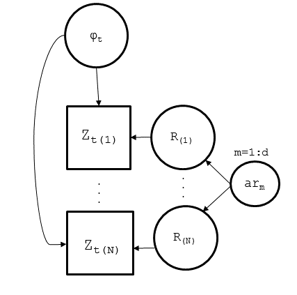
Figure 5: Part of the DAG representation of the full model given in Figure 4 that is modified to account for multiple trials.

Appendix N Granger-Causality Detection Results

N.1 Data generated with slowly-varying parameters and normal errors

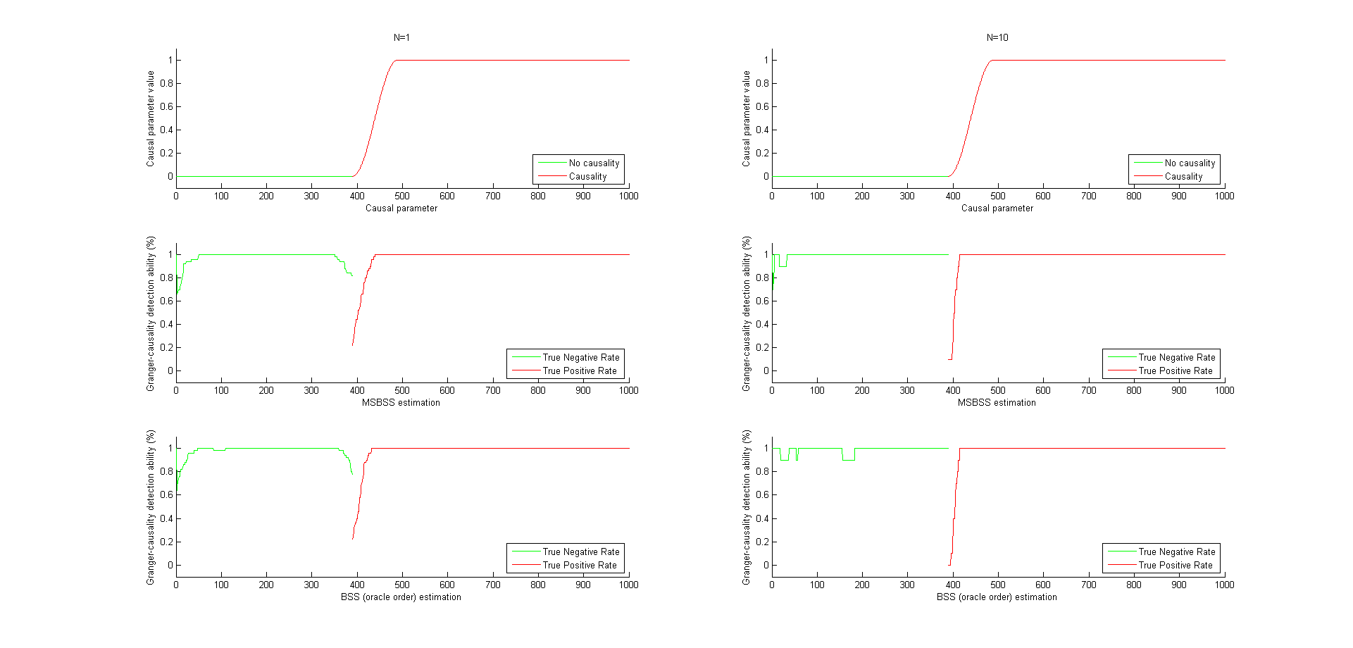
Figure 6: Granger-causality detection ability for order $1$, series length $1000$ and causal parameter $1$.

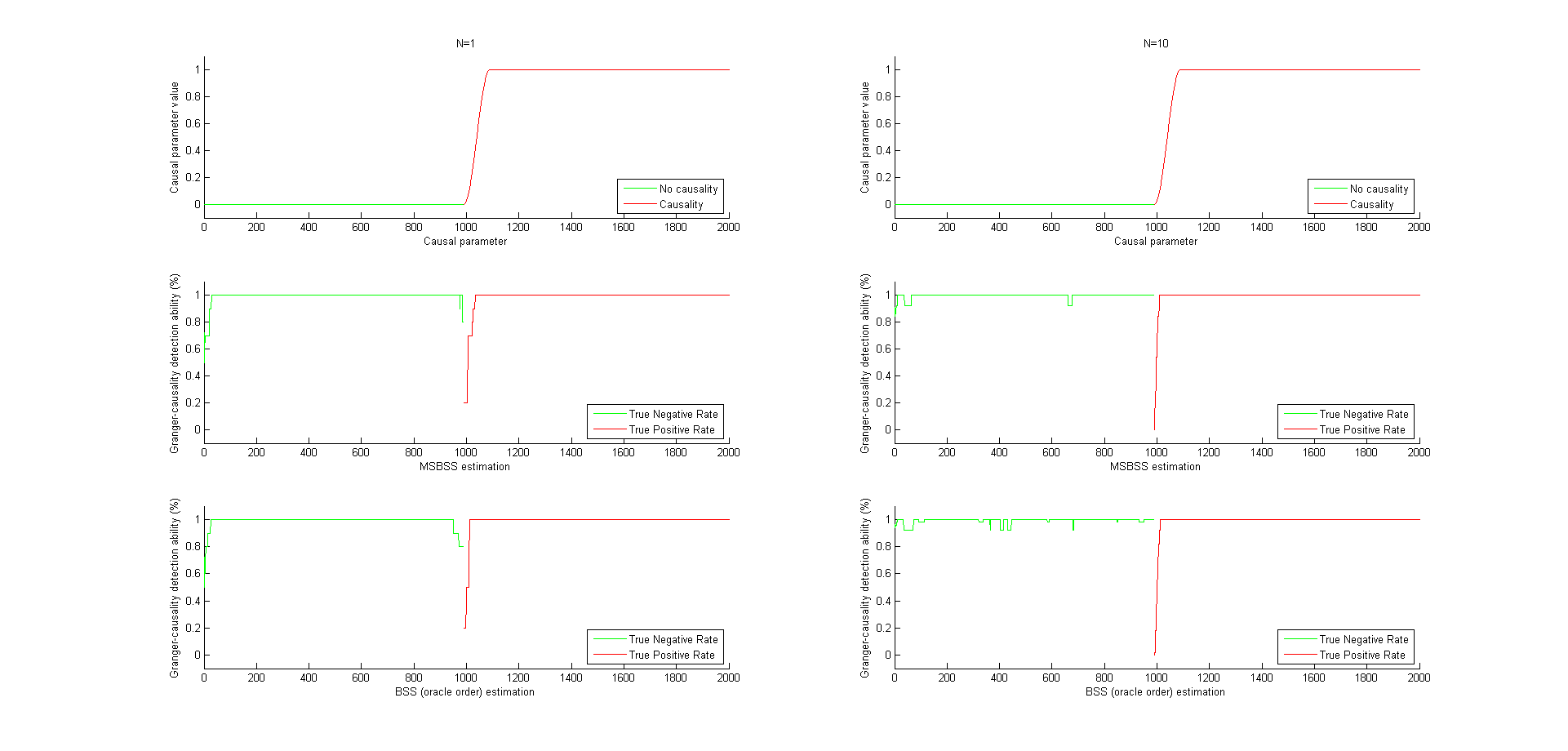
Figure 7: Granger-causality detection ability for order $1$, series length $2000$ and causal parameter $1$.

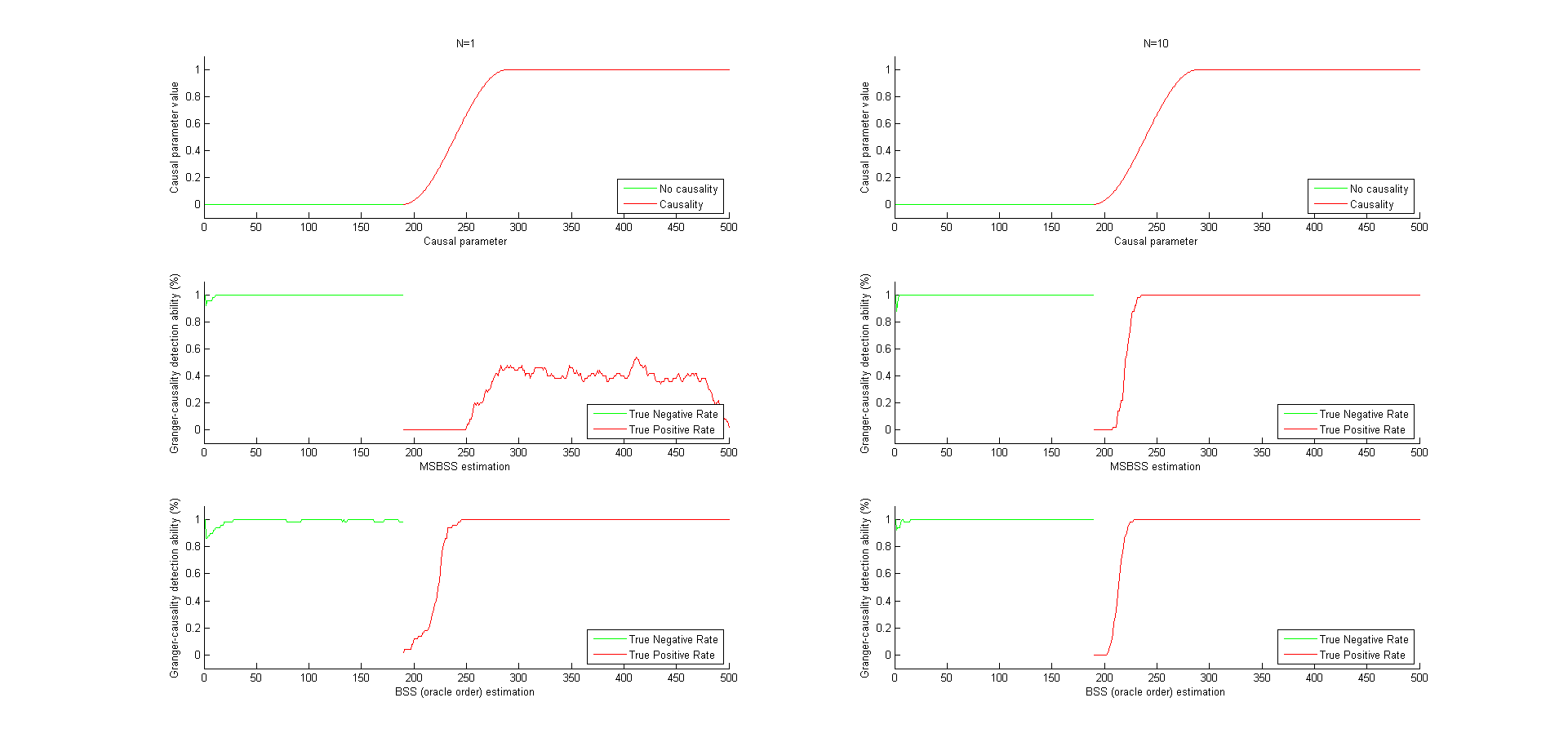
Figure 8: Granger-causality detection ability for order $2$, series length $500$ and causal parameter $1$.

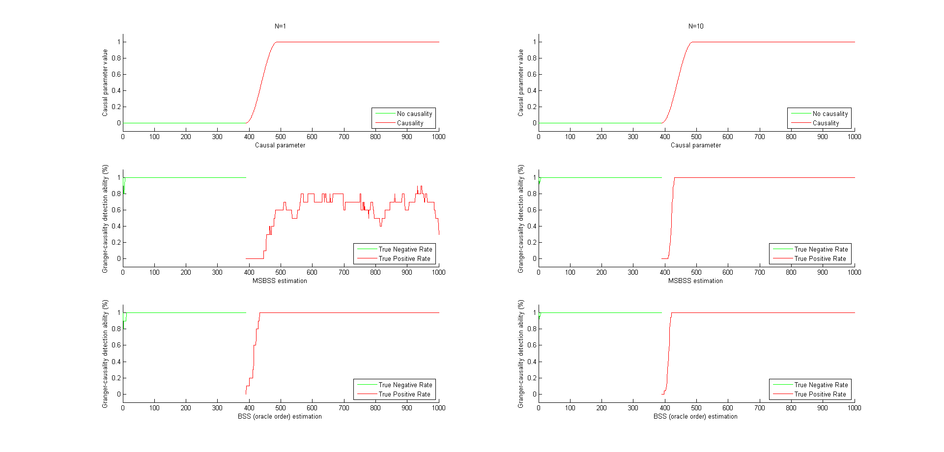
Figure 9: Granger-causality detection ability for order $2$, series length $1000$ and causal parameter $1$.

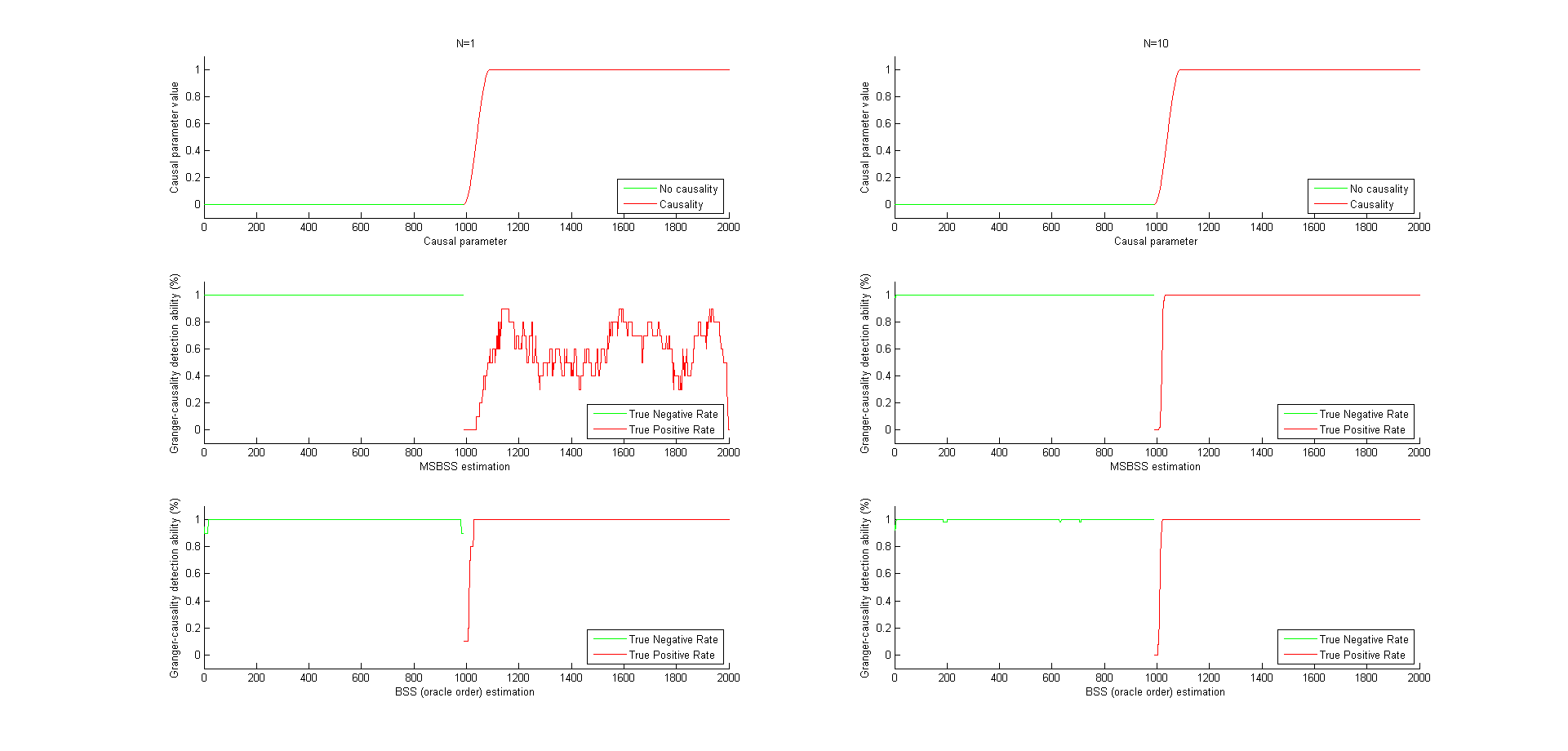
Figure 10: Granger-causality detection ability for order $2$, series length $2000$ and causal parameter $1$.

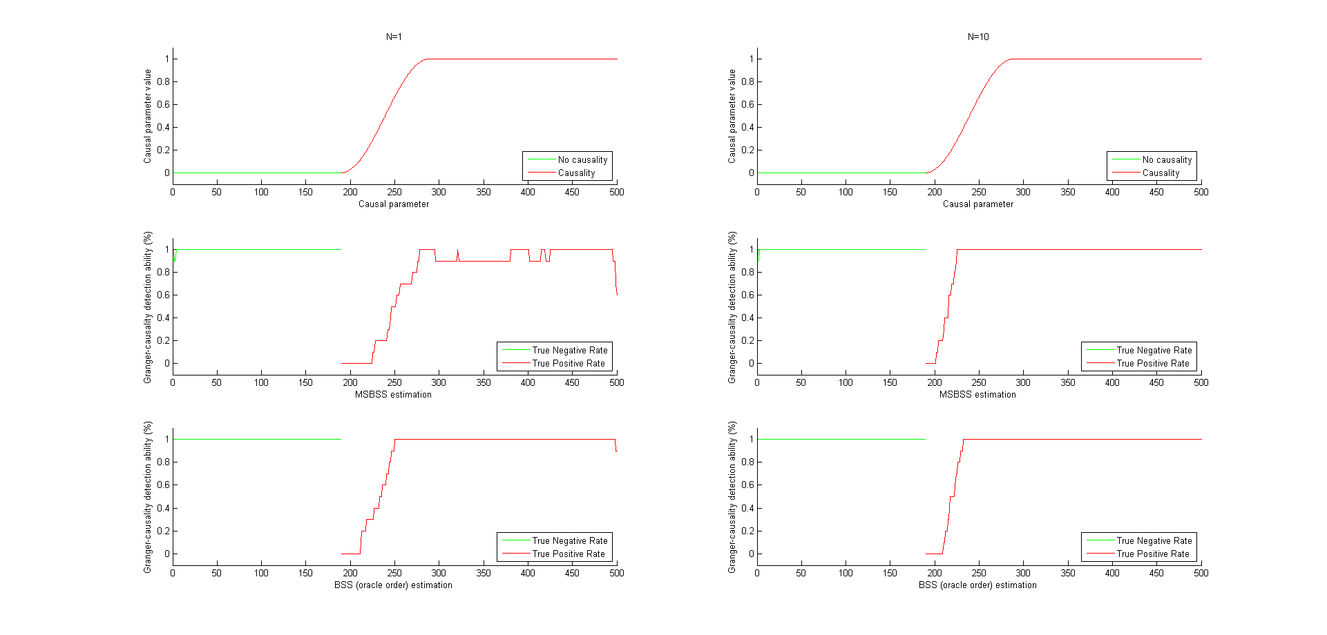
Figure 11: Granger-causality detection ability for order $4$, series length $500$ and causal parameter $1$.

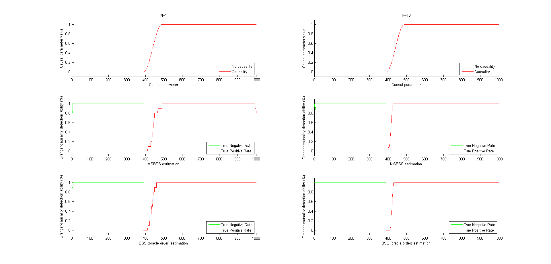
Figure 12: Granger-causality detection ability for order $4$, series length $1000$ and causal parameter $1$.

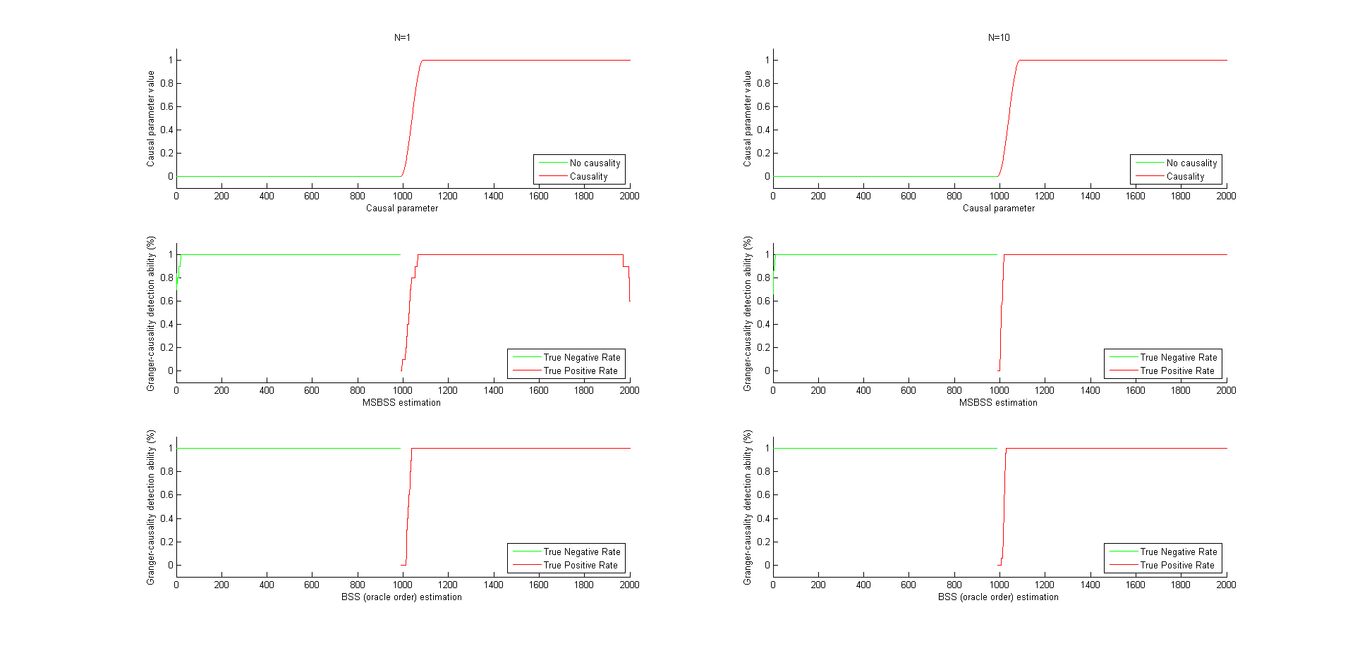
Figure 13: Granger-causality detection ability for order $4$, series length $2000$ and causal parameter $1$.

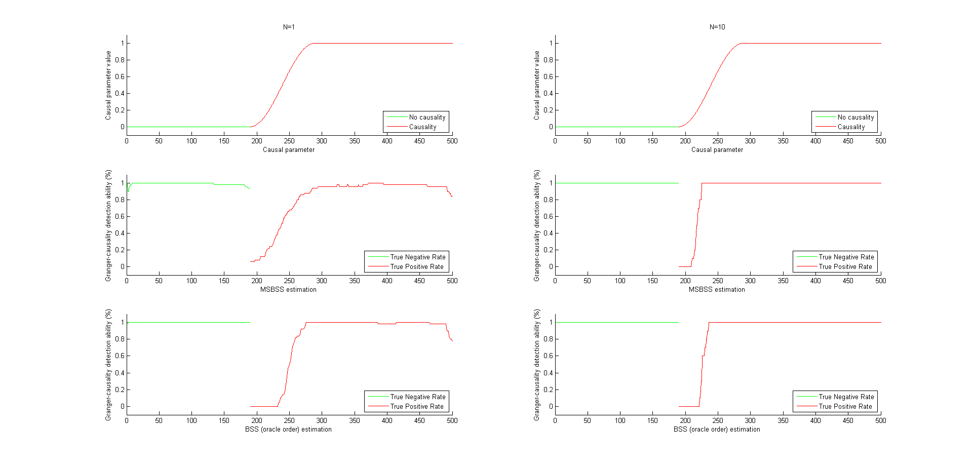
Figure 14: Granger-causality detection ability for order $8$, series length $500$ and causal parameter $1$.

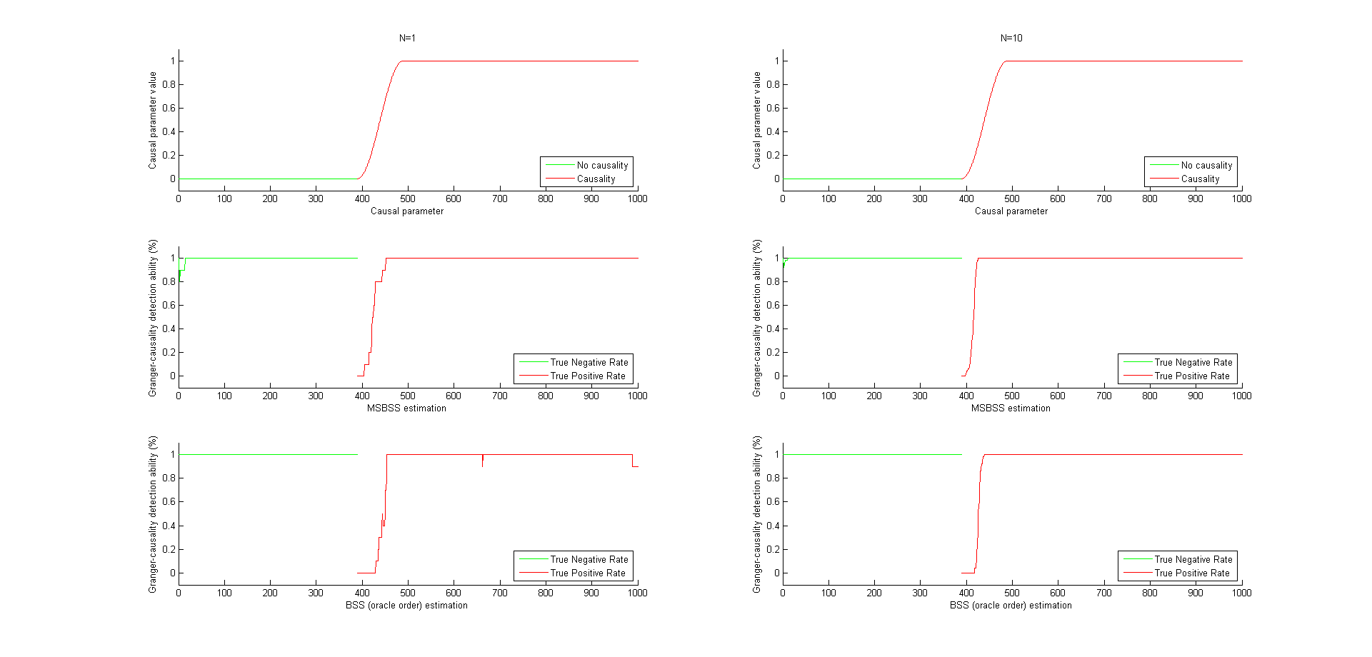
Figure 15: Granger-causality detection ability for order $8$, series length $1000$ and causal parameter $1$.

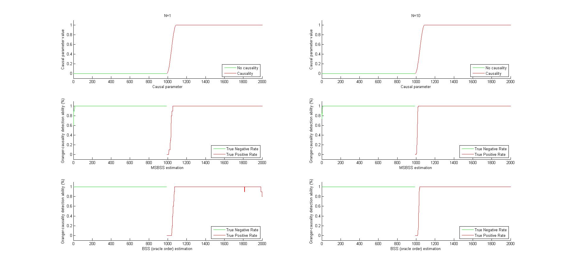
Figure 16: Granger-causality detection ability for order $8$, series length $2000$ and causal parameter $1$.

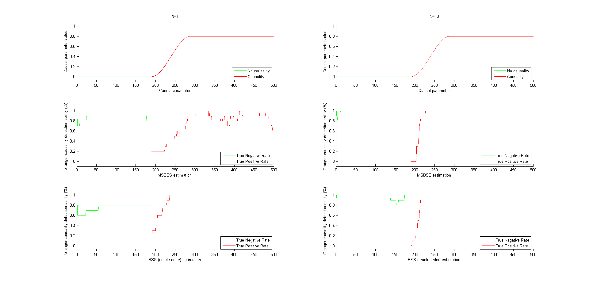
Figure 17: Granger-causality detection ability for order $1$, series length $500$ and causal parameter $0.8$.

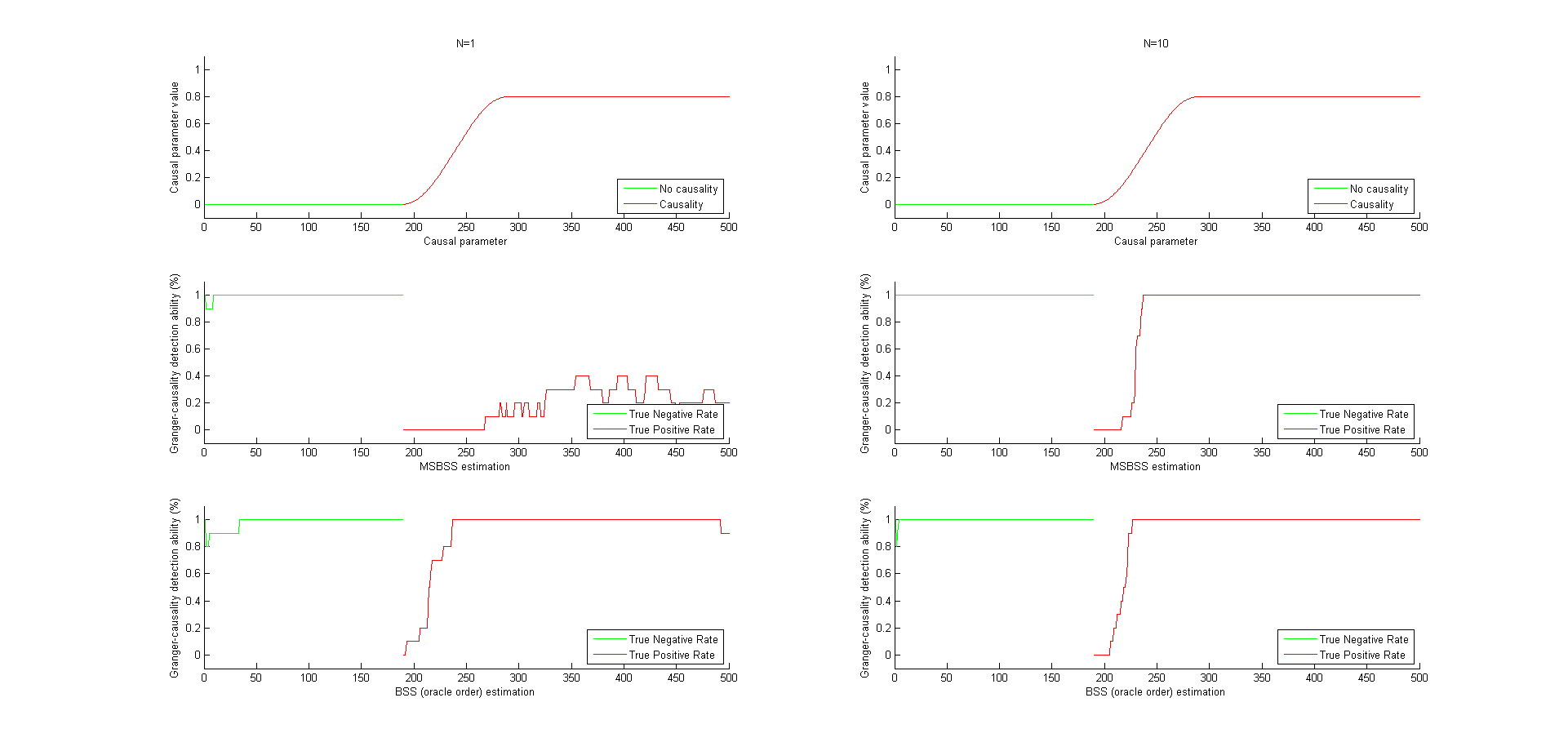
Figure 18: Granger-causality detection ability for order $2$, series length $500$ and causal parameter $0.8$.

Figure 19: Granger-causality detection ability for order $4$, series length $500$ and causal parameter $0.8$.

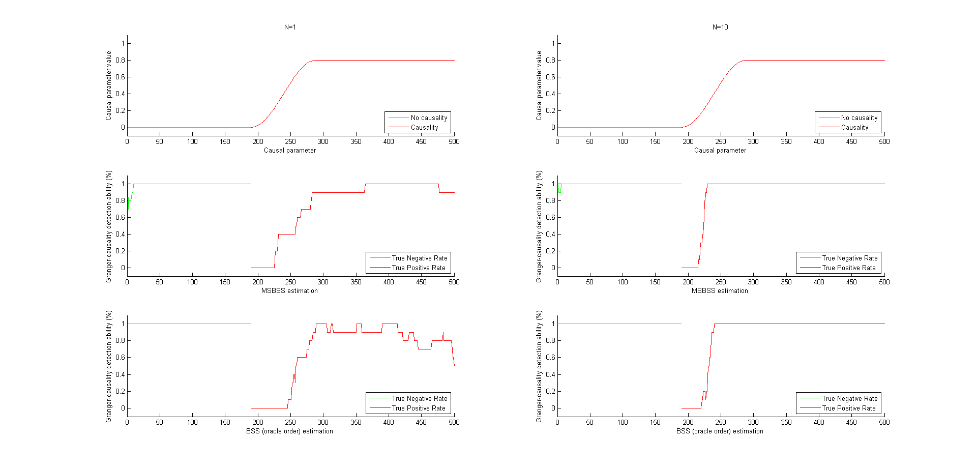
Figure 20: Granger-causality detection ability for order $8$, series length $500$ and causal parameter $0.8$.

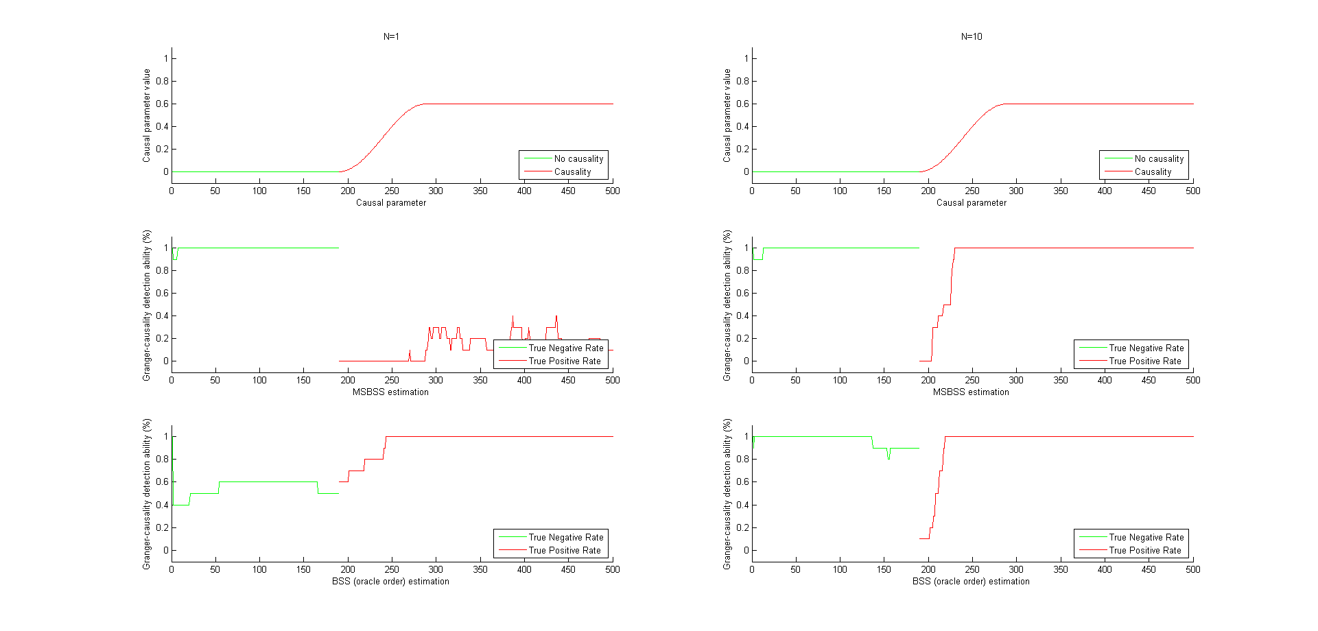
Figure 21: Granger-causality detection ability for order $1$, series length $500$ and causal parameter $0.6$.

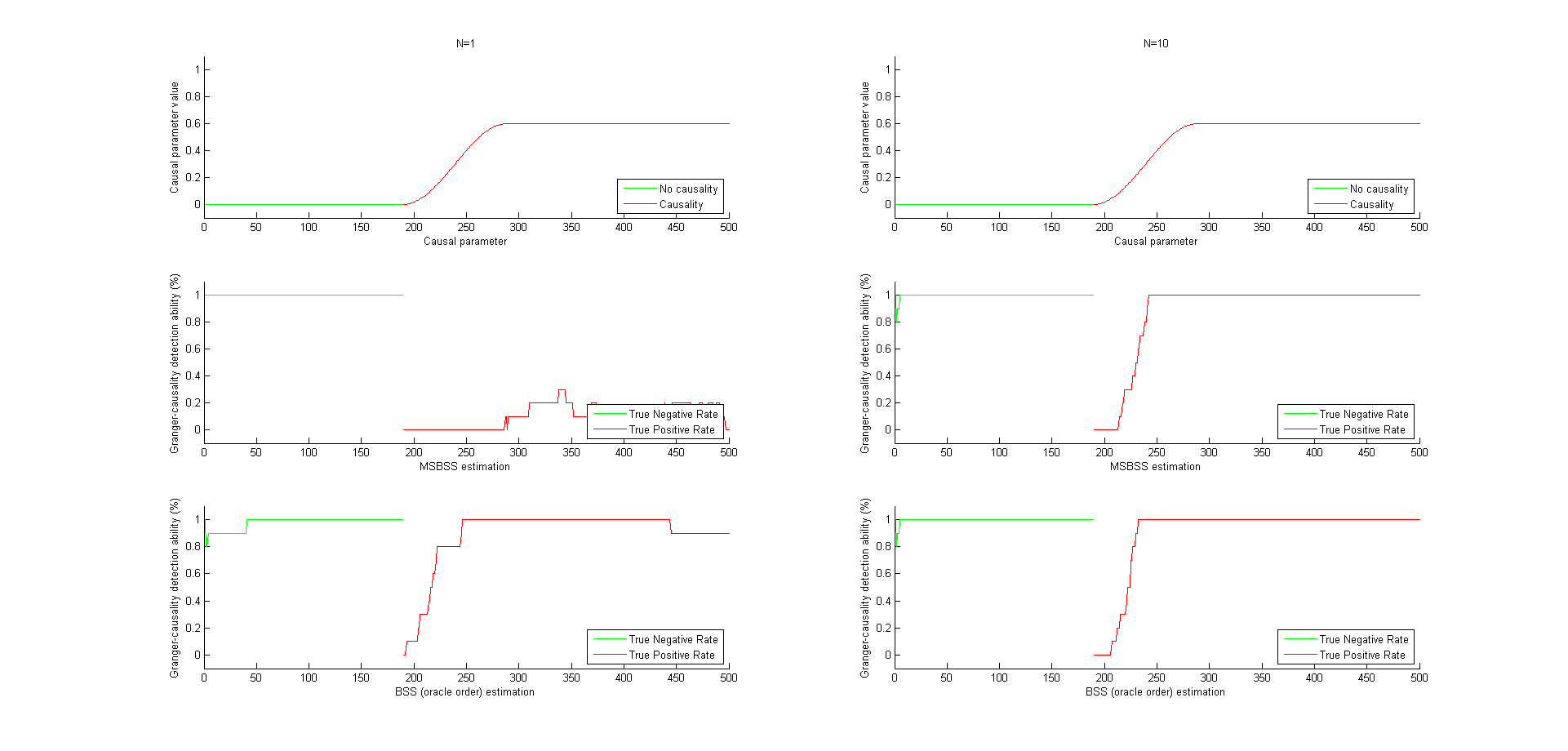
Figure 22: Granger-causality detection ability for order $2$, series length $500$ and causal parameter $0.6$.

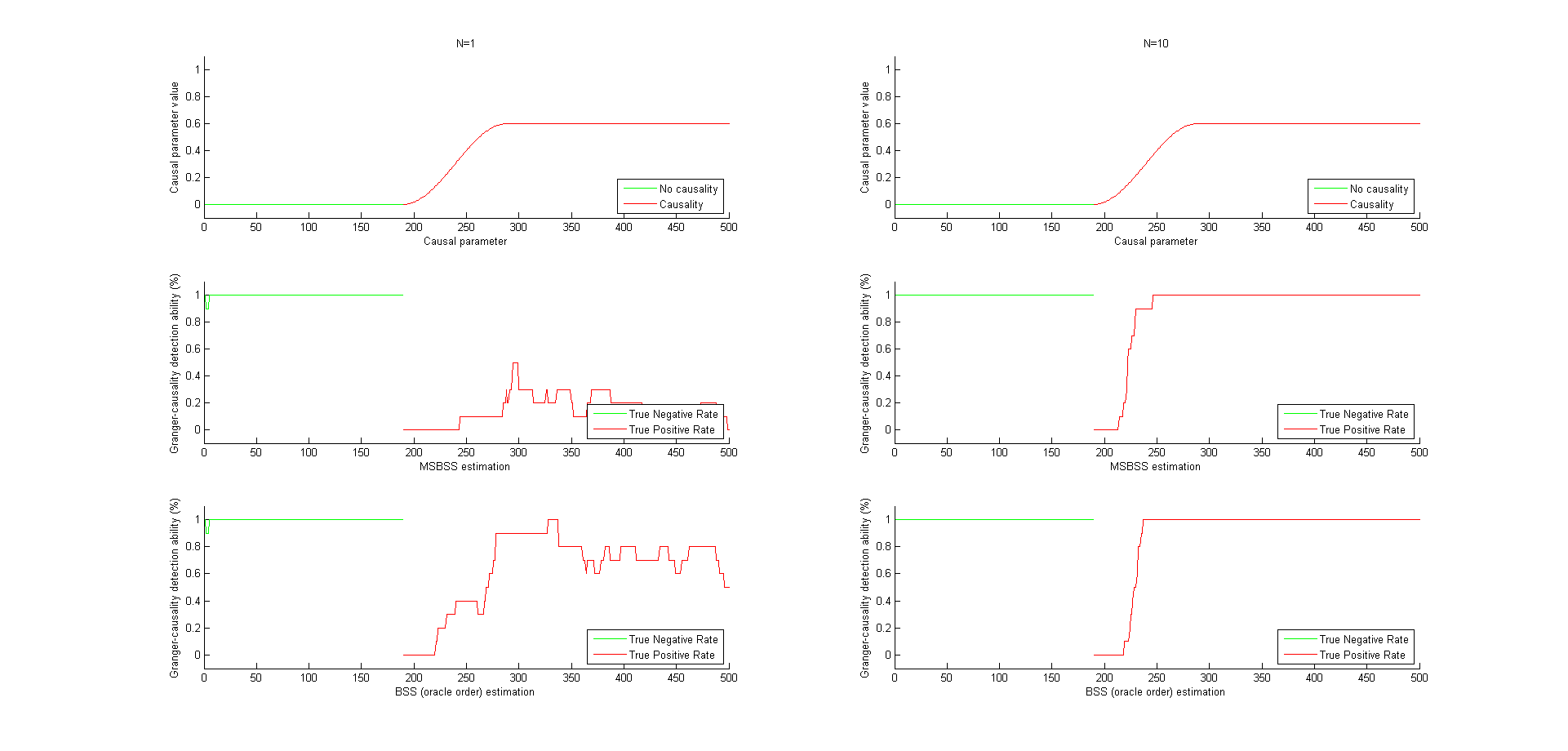
Figure 23: Granger-causality detection ability for order $4$, series length $500$ and causal parameter $0.6$.

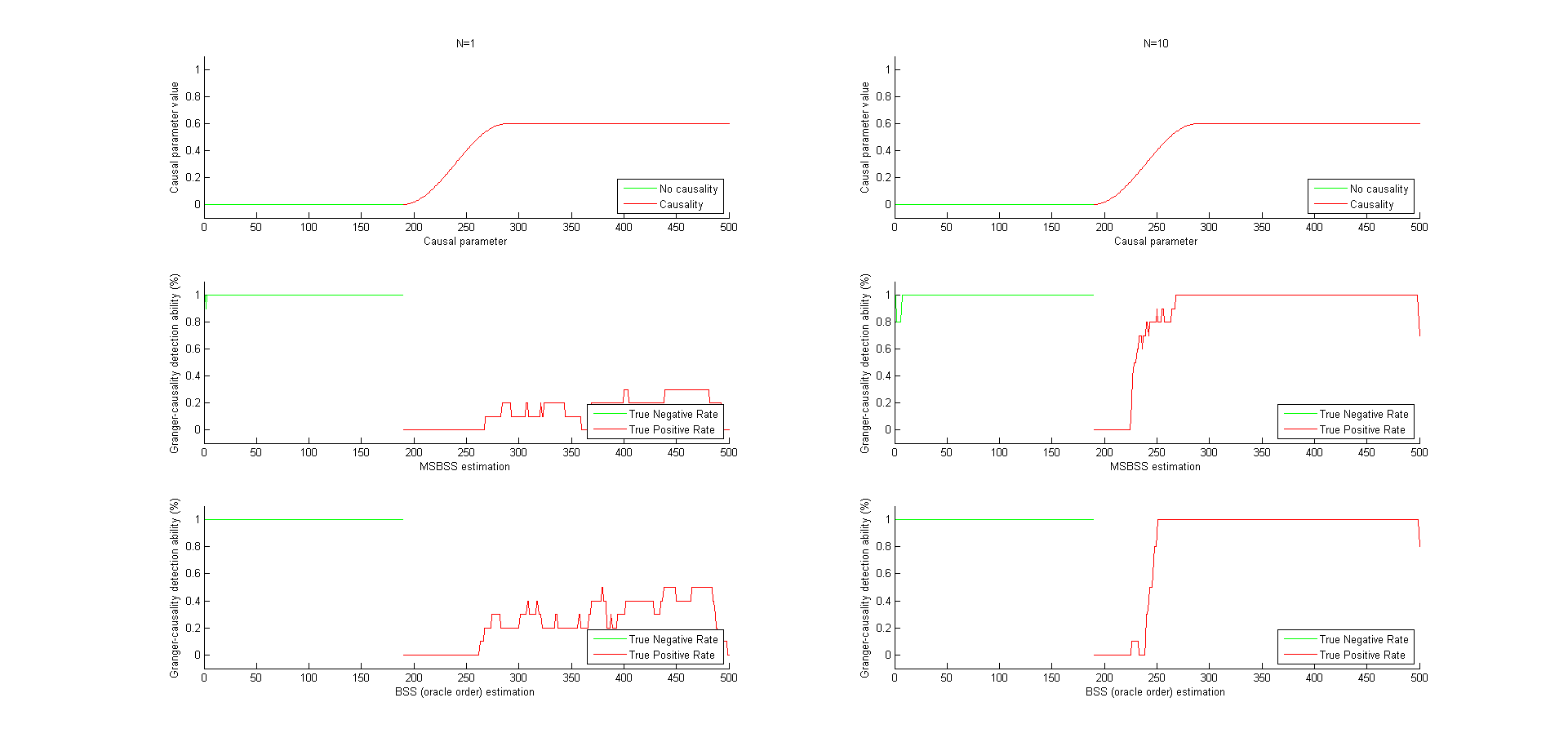
Figure 24: Granger-causality detection ability for order $8$, series length $500$ and causal parameter $0.6$.

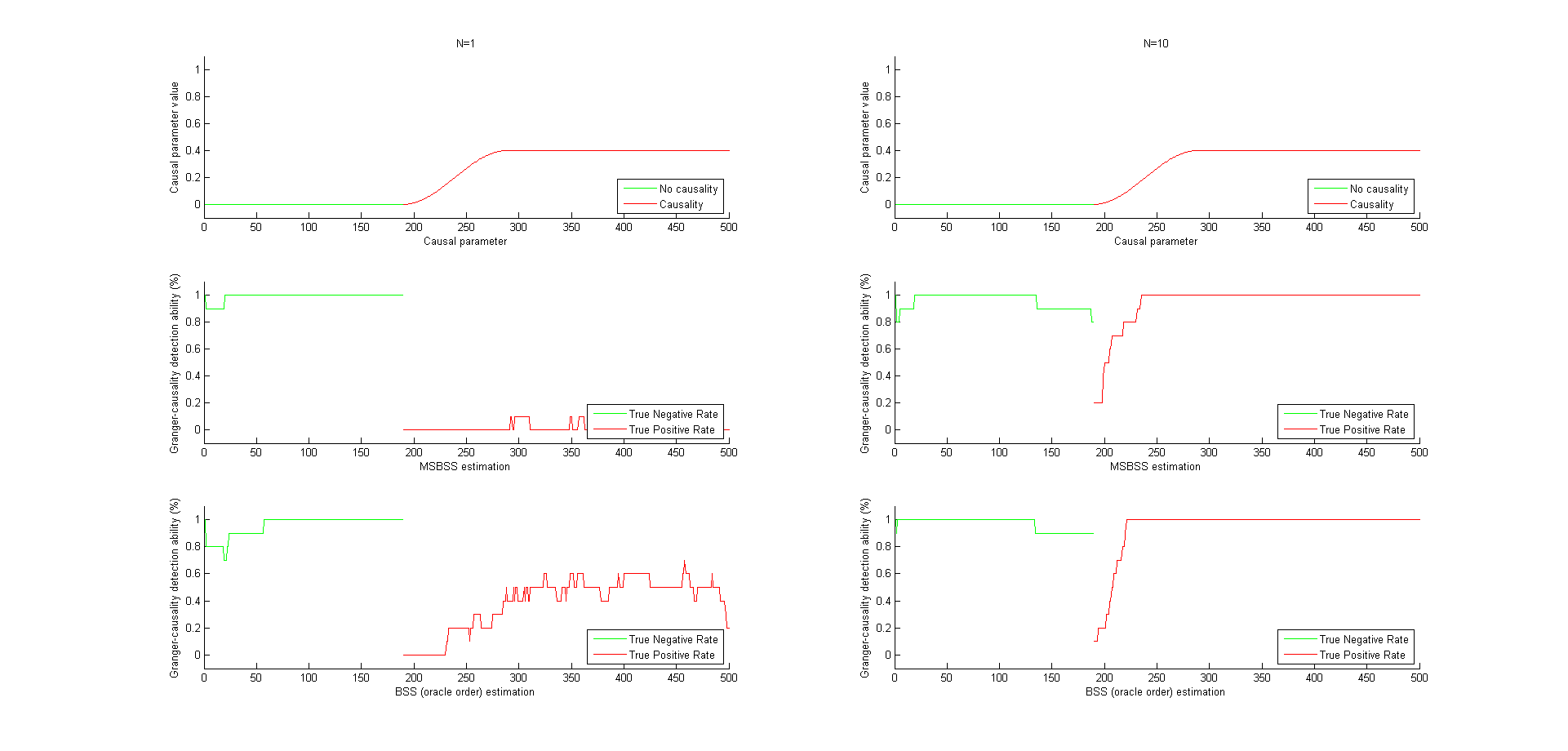
Figure 25: Granger-causality detection ability for order $1$, series length $500$ and causal parameter $0.4$.

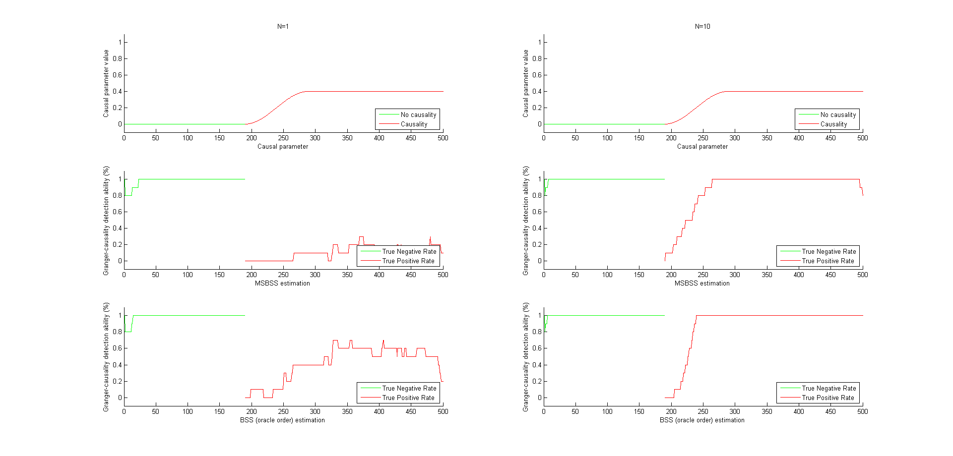
Figure 26: Granger-causality detection ability for order $2$, series length $500$ and causal parameter $0.4$.

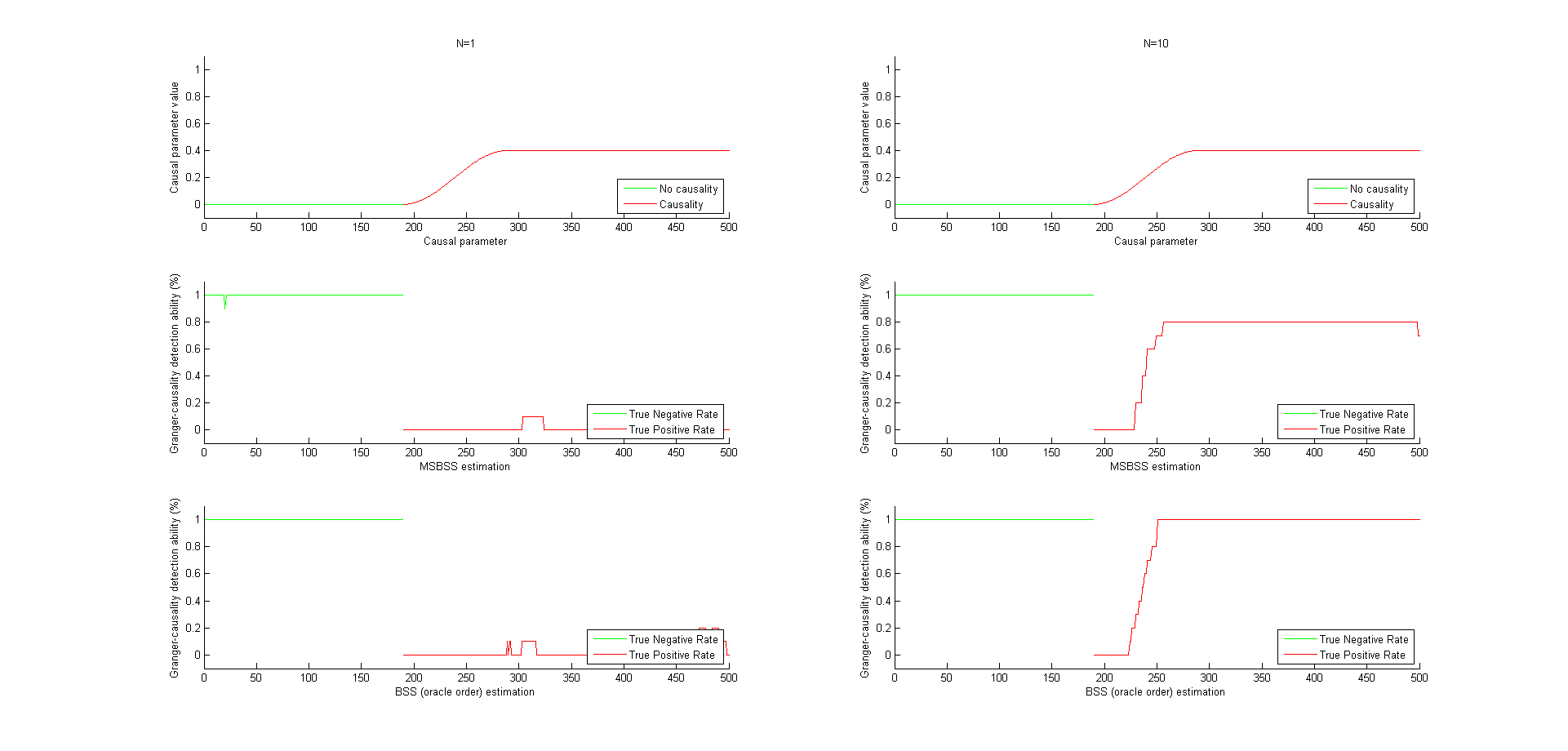
Figure 27: Granger-causality detection ability for order $4$, series length $500$ and causal parameter $0.4$.

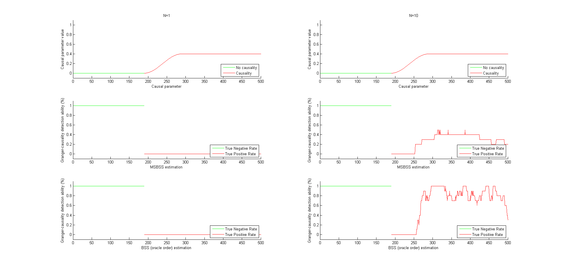
Figure 28: Granger-causality detection ability for order $8$, series length $500$ and causal parameter $0.4$.

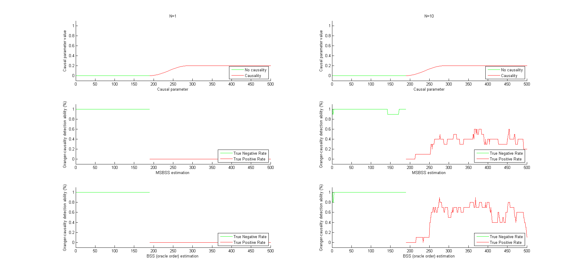
Figure 29: Granger-causality detection ability for order $2$, series length $500$ and causal parameter $0.2$.

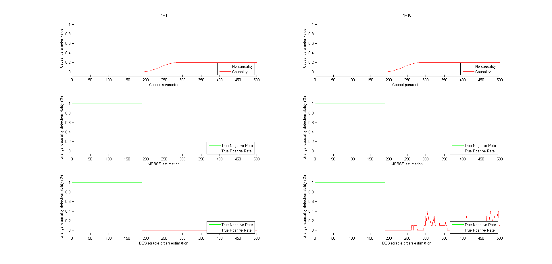
Figure 30: Granger-causality detection ability for order $4$, series length $500$ and causal parameter $0.2$.

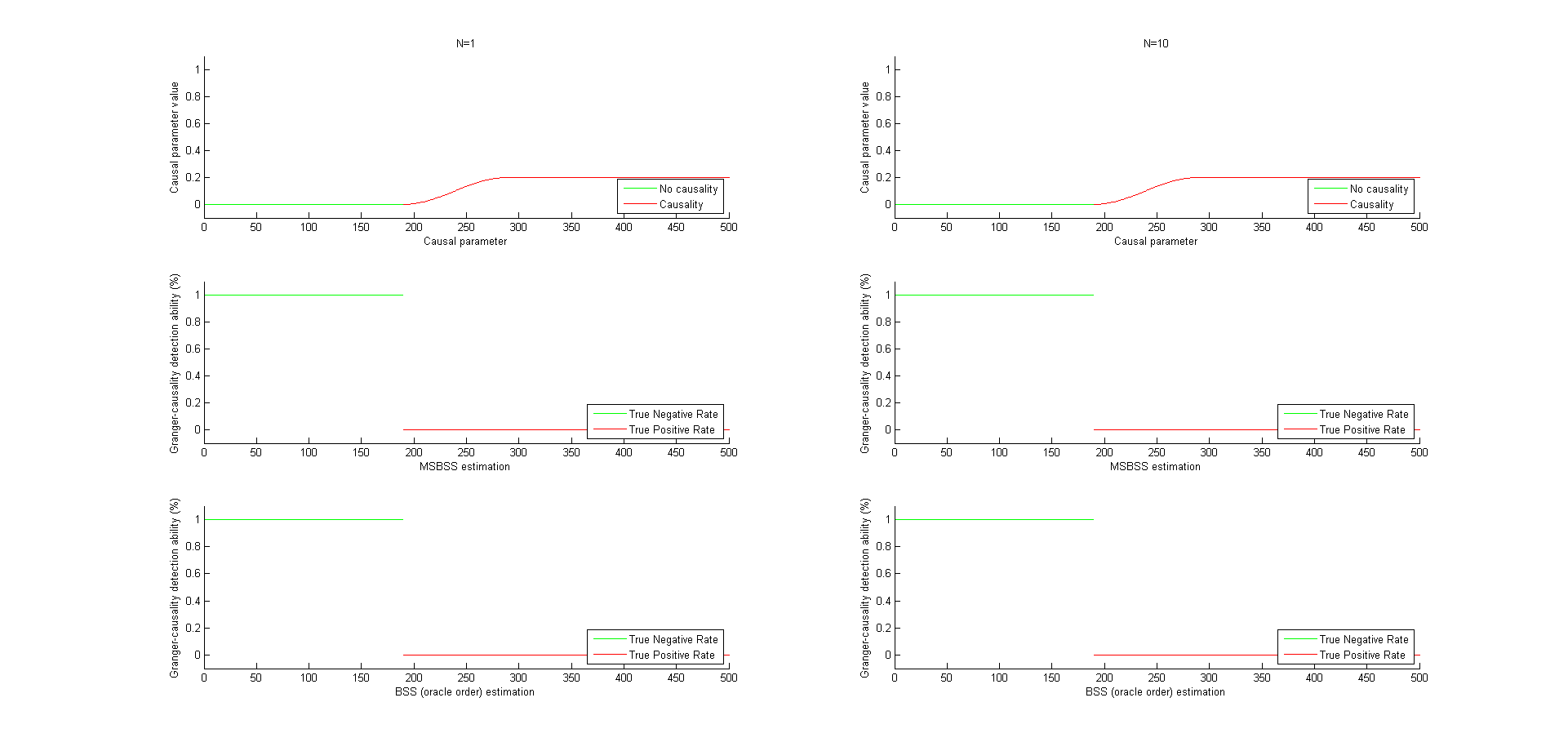
Figure 31: Granger-causality detection ability for order $8$, series length $500$ and causal parameter $0.2$.

N.2 Data generated with slowly-varying parameters and non-normal errors

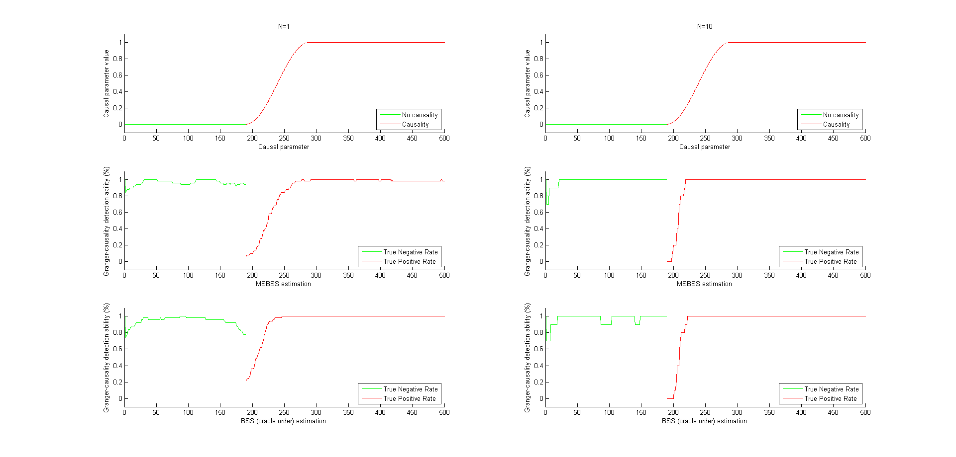
Figure 32: Granger-causality detection ability for a non-normal error simulation of order $1$, series length $500$ and causal parameter $1$.

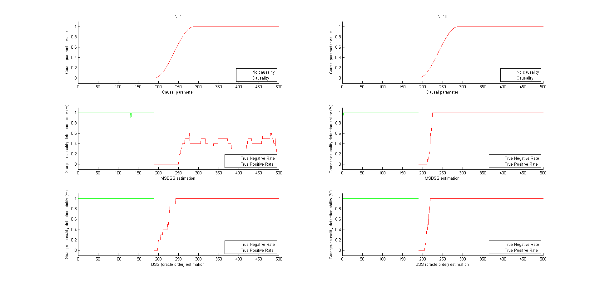
Figure 33: Granger-causality detection ability for a non-normal error simulation of order $2$ and series length $500$ and causal parameter $1$.

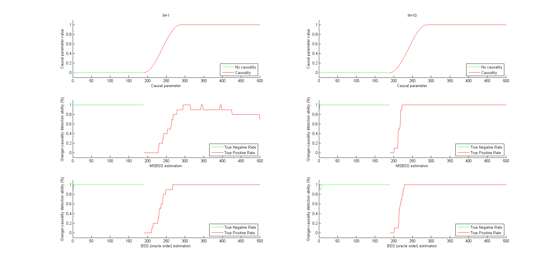
Figure 34: Granger-causality detection ability for a non-normal error simulation of order $4$ and series length $500$ and causal parameter $1$.

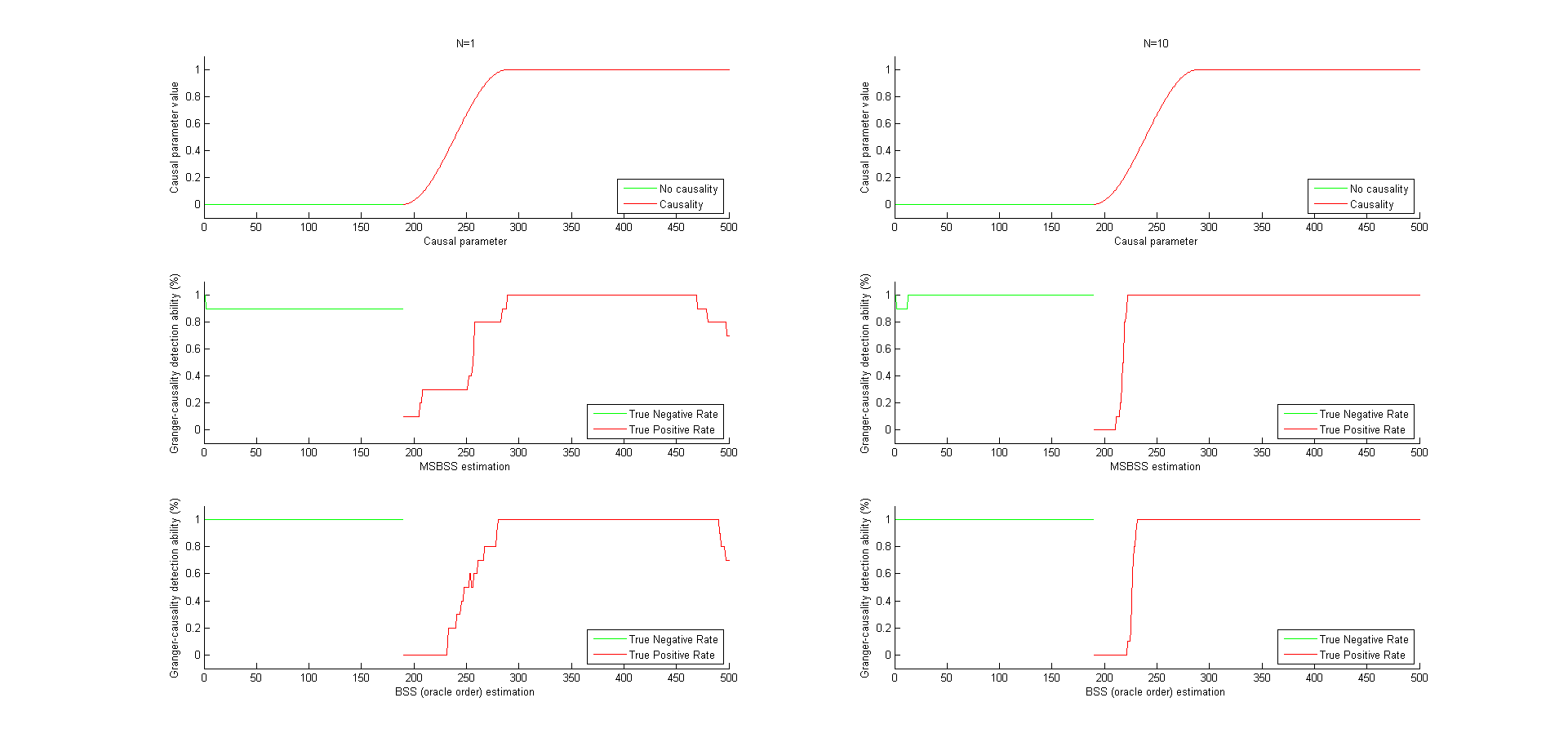
Figure 35: Granger-causality detection ability for a non-normal error simulation of order $8$ and series length $500$ and causal parameter $1$.

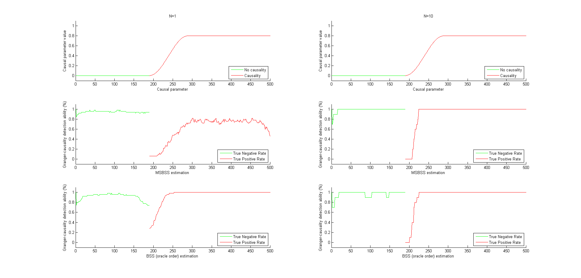
Figure 36: Granger-causality detection ability for a non-normal error simulation of order $1$ and series length $500$ and causal parameter $0.8$.

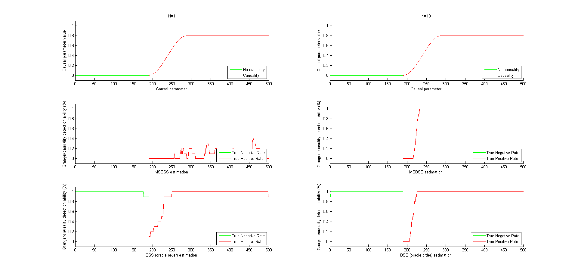
Figure 37: Granger-causality detection ability for a non-normal error simulation of order $2$ and series length $500$ and causal parameter $0.8$.

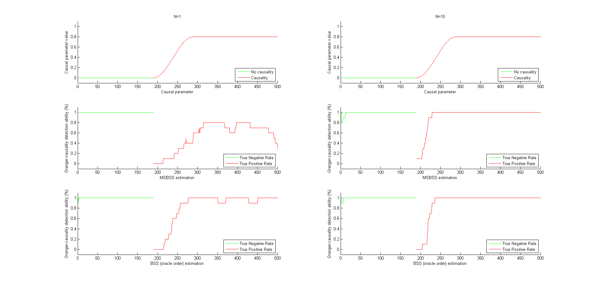
Figure 38: Granger-causality detection ability for a non-normal error simulation of order $4$ and series length $500$ and causal parameter $0.8$.

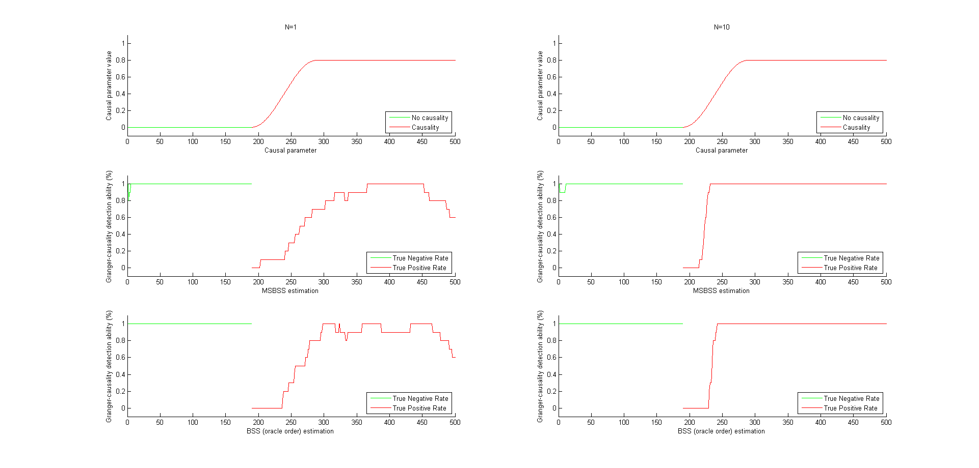
Figure 39: Granger-causality detection ability for a non-normal error simulation of order $8$ and series length $500$ and causal parameter $0.8$.

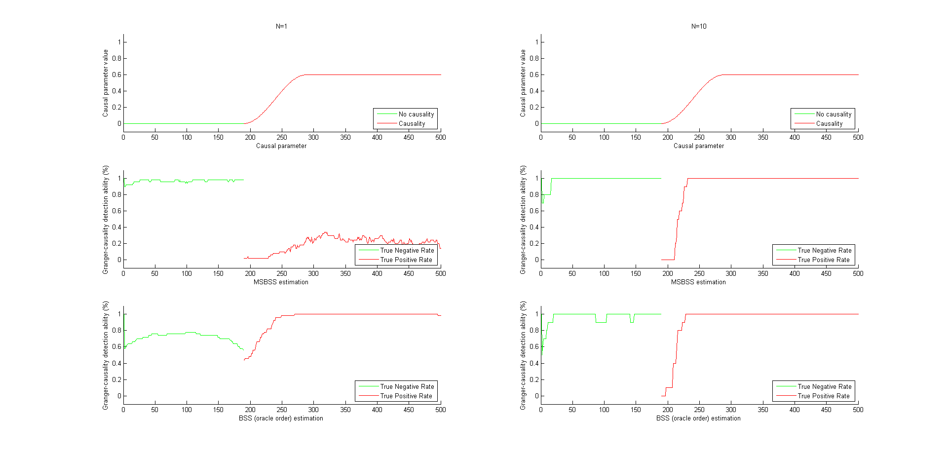
Figure 40: Granger-causality detection ability for a non-normal error simulation of order $1$ and series length $500$ and causal parameter $0.6$.

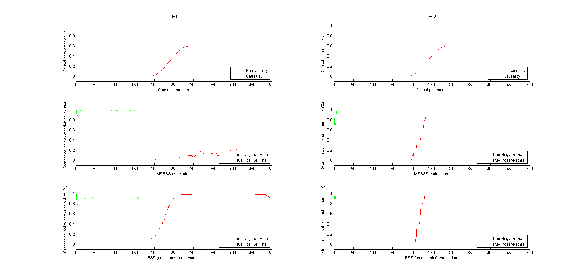
Figure 41: Granger-causality detection ability for a non-normal error simulation of order $2$ and series length $500$ and causal parameter $0.6$.

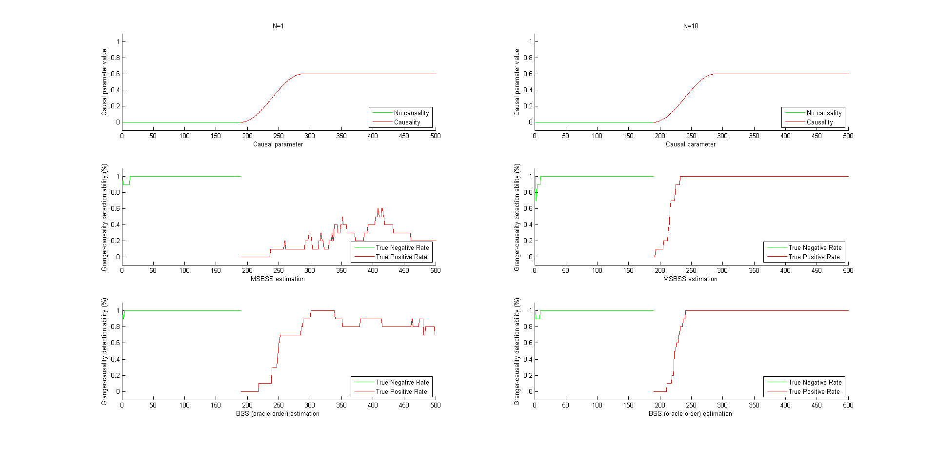
Figure 42: Granger-causality detection ability for a non-normal error simulation of order $4$ and series length $500$ and causal parameter $0.6$.

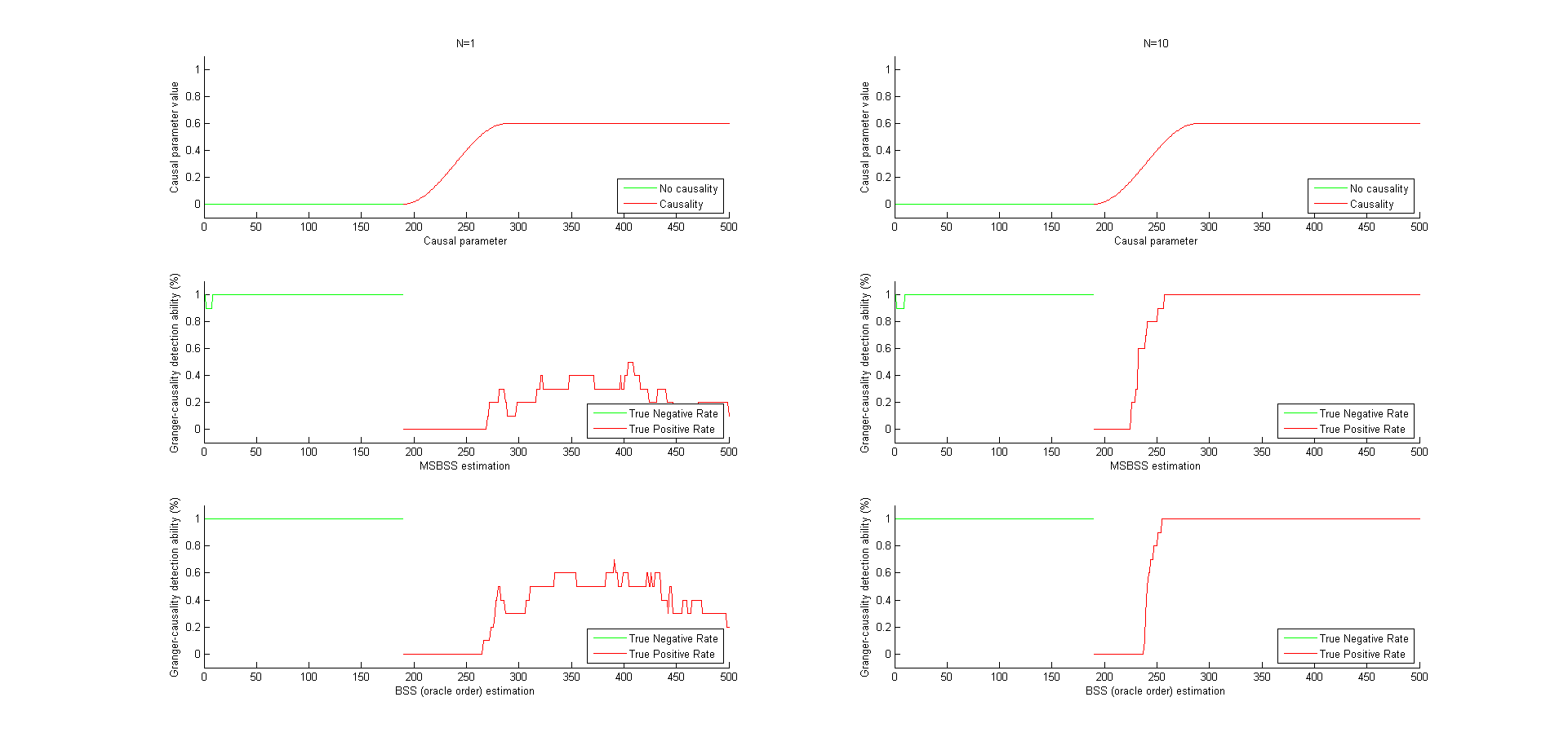
Figure 43: Granger-causality detection ability for a non-normal error simulation of order $8$ and series length $500$ and causal parameter $0.6$.

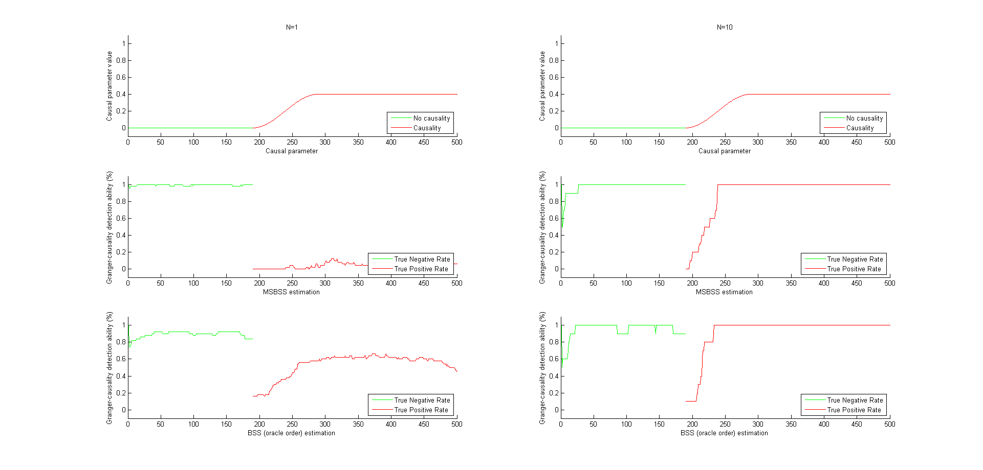
Figure 44: Granger-causality detection ability for a non-normal error simulation of order $1$, series length $500$ and causal parameter $0.4$.

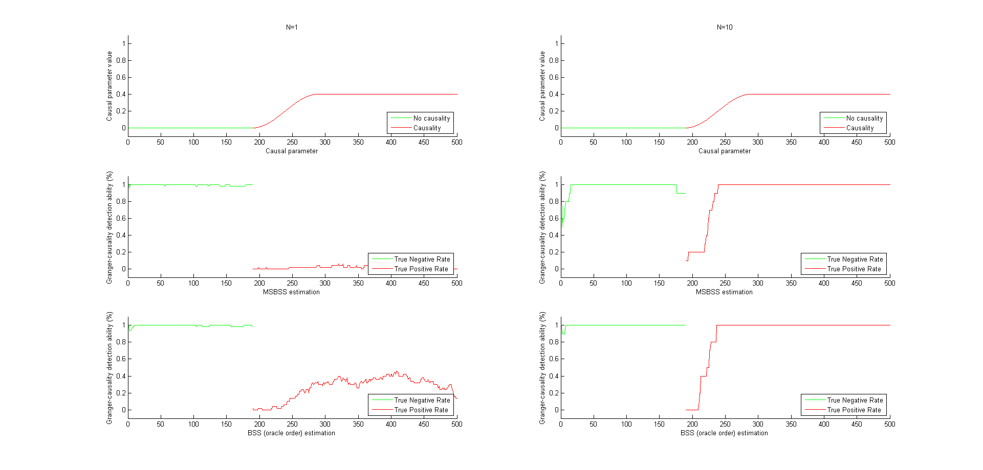
Figure 45: Granger-causality detection ability for a non-normal error simulation of order $2$ and series length $500$ and causal parameter $0.4$.

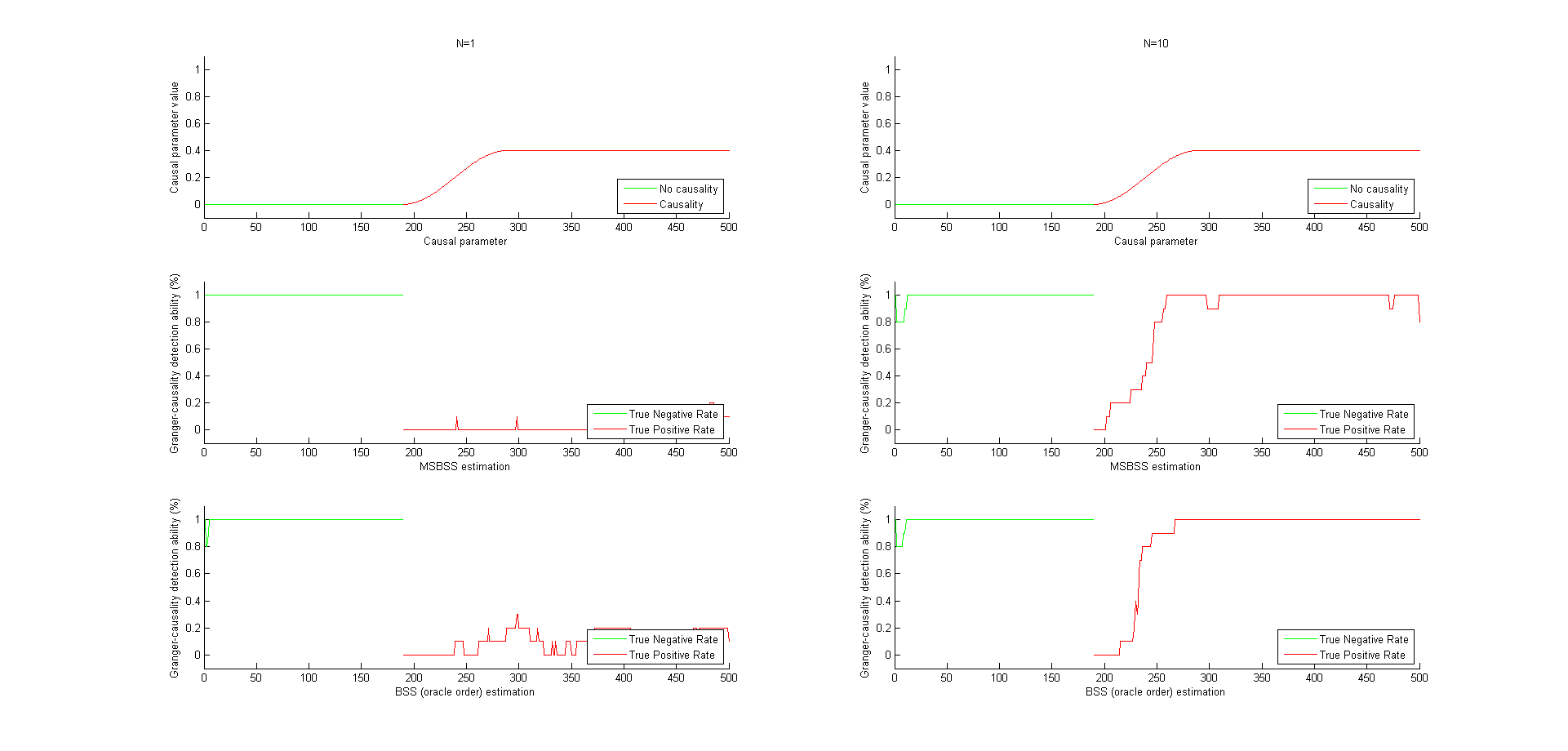
Figure 46: Granger-causality detection ability for a non-normal error simulation of order $4$ and series length $500$ and causal parameter $0.4$.

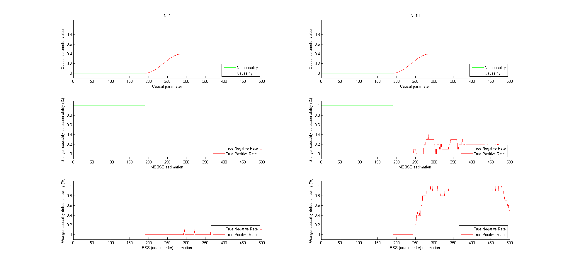
Figure 47: Granger-causality detection ability for a non-normal error simulation of order $8$ and series length $500$ and causal parameter $0.4$.

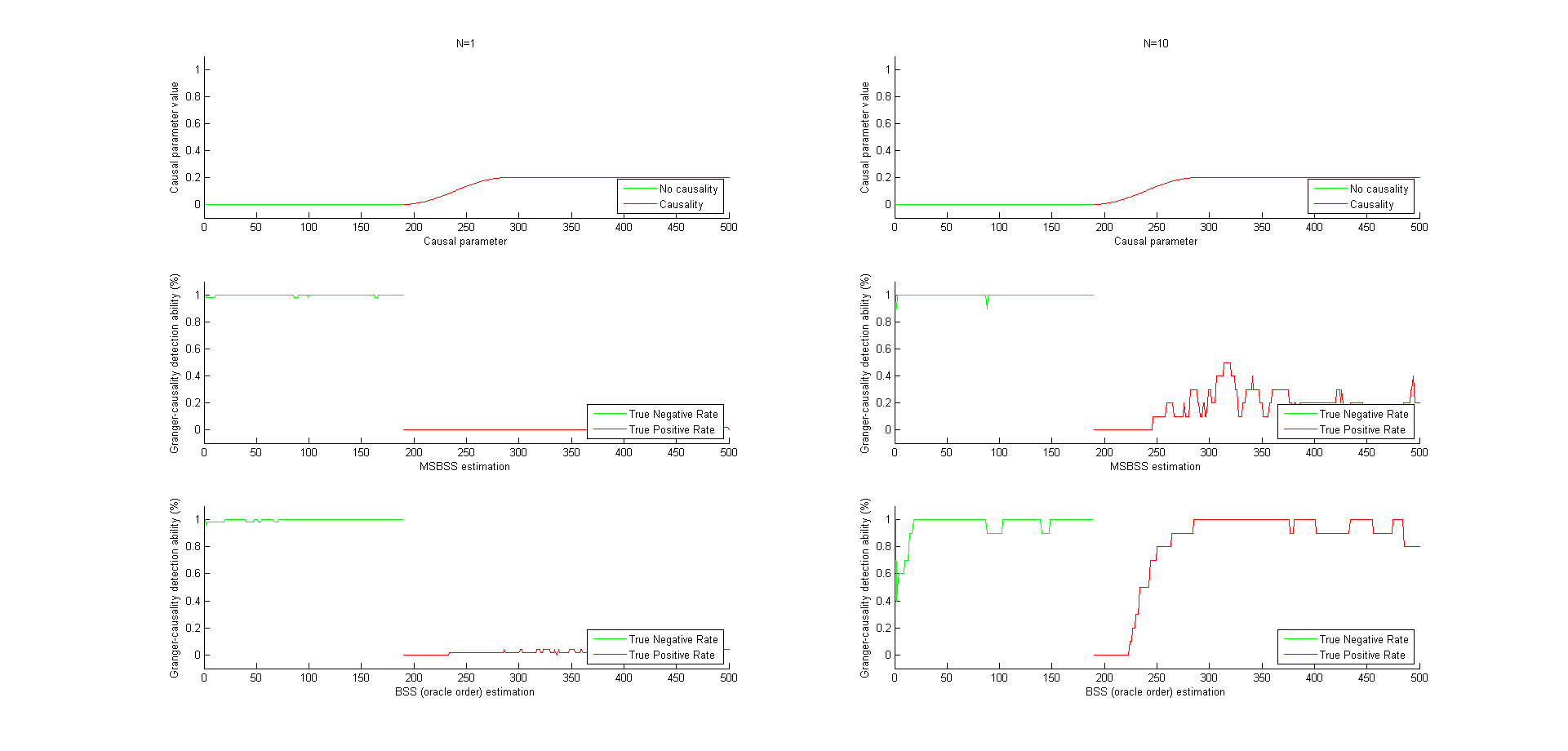
Figure 48: Granger-causality detection ability for a non-normal error simulation of order $1$ and series length $500$ and causal parameter $0.2$.

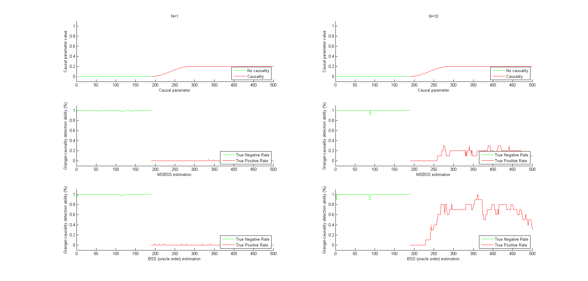
Figure 49: Granger-causality detection ability for a non-normal error simulation of order $2$ and series length $500$ and causal parameter $0.2$.

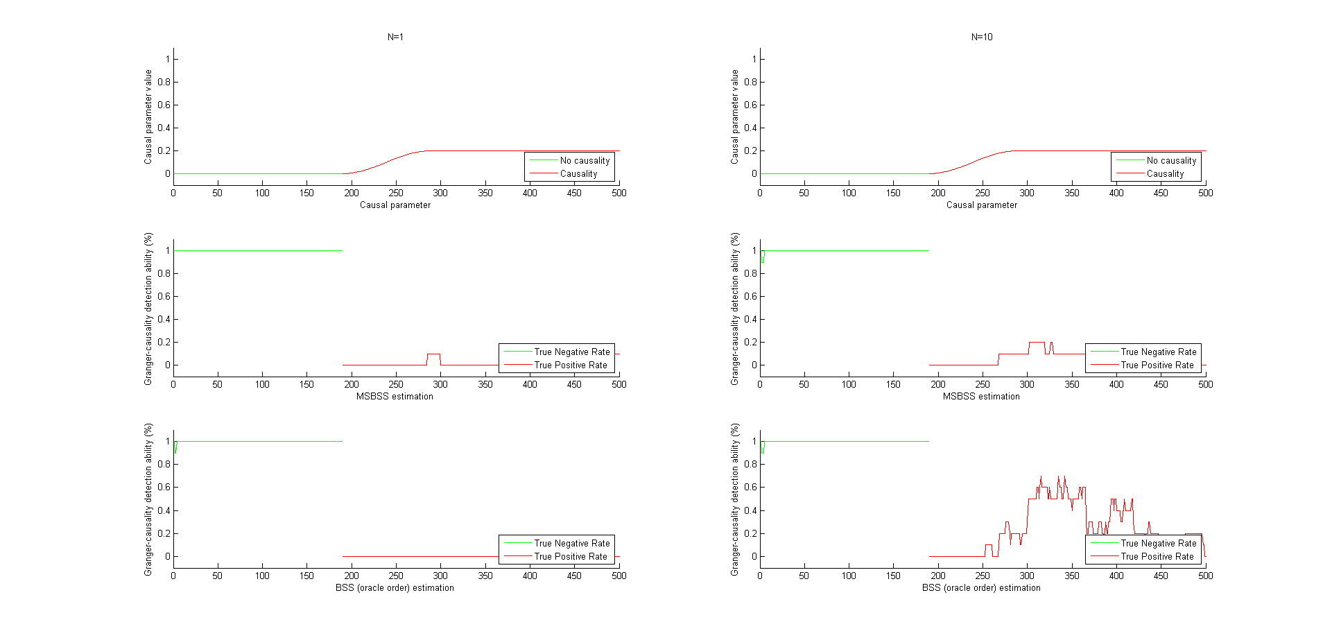
Figure 50: Granger-causality detection ability for a non-normal error simulation of order $4$ and series length $500$ and causal parameter $0.2$.

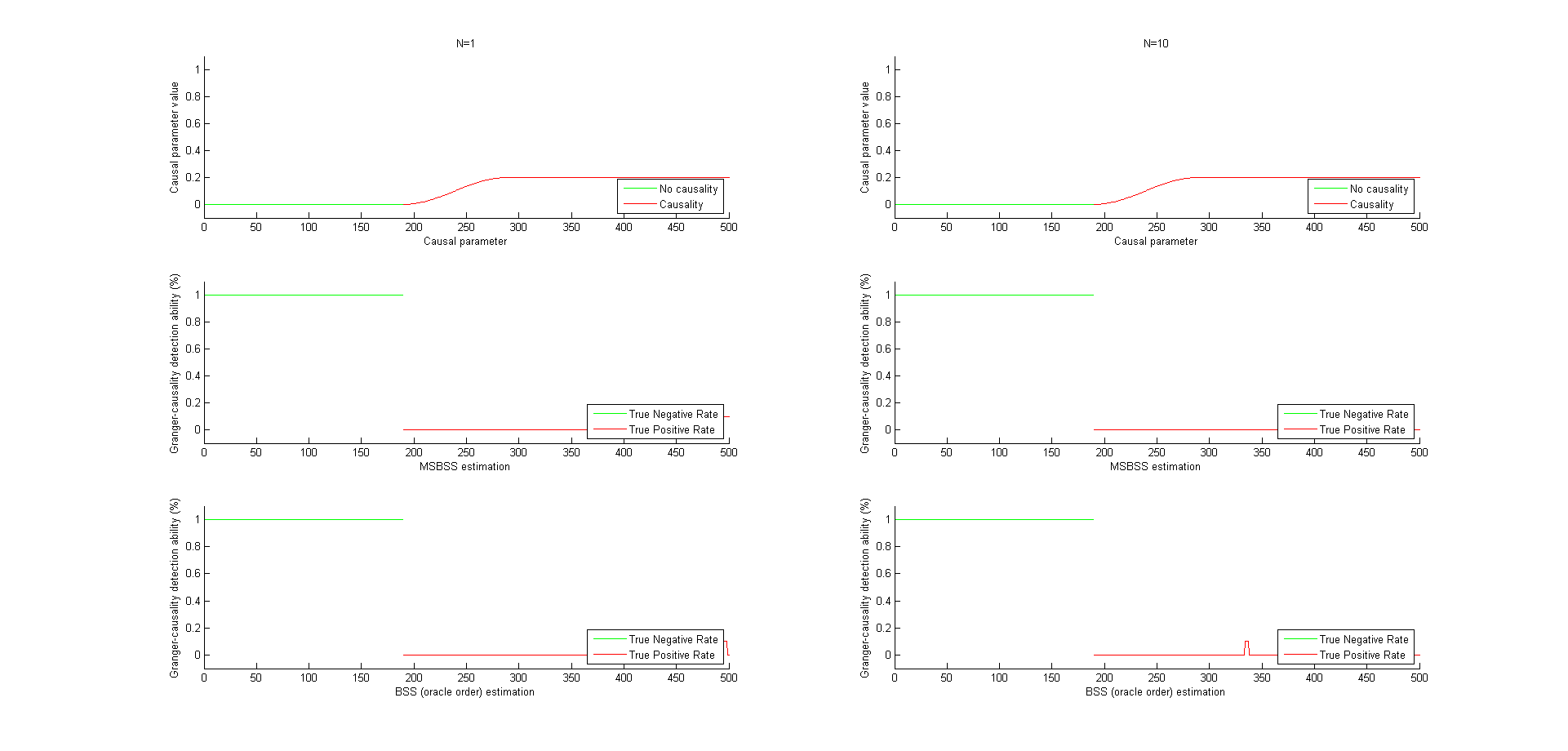
Figure 51: Granger-causality detection ability for a non-normal error simulation of order $8$ and series length $500$ and causal parameter $0.2$.

N.3 Windowing estimation procedure

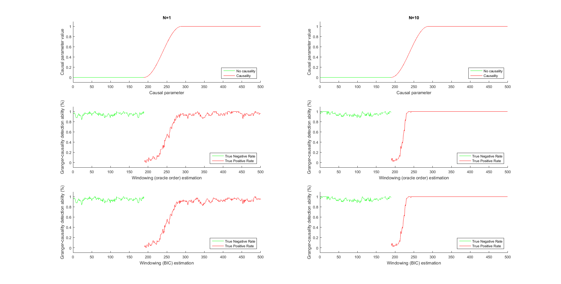
Figure 52: Granger-causality detection ability for a windowing estimation procedure with a model order $1$, series length $500$ and causal parameter $1$. The middle graphs show the results for the true model order estimate (oracle) and the bottom graphs those for the model order selected based on the BIC criterion.

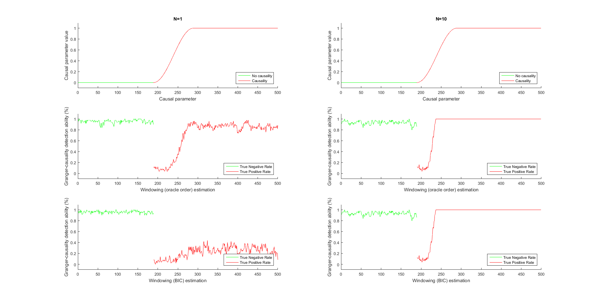
Figure 53: Granger-causality detection ability for a windowing estimation procedure with a model order $2$ and series length $500$ and causal parameter $1$.

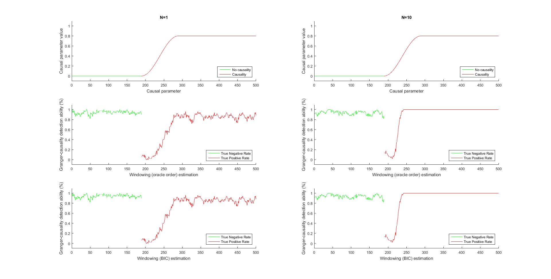
Figure 54: Granger-causality detection ability for a windowing estimation procedure with a model order $1$ and series length $500$ and causal parameter $0.8$.

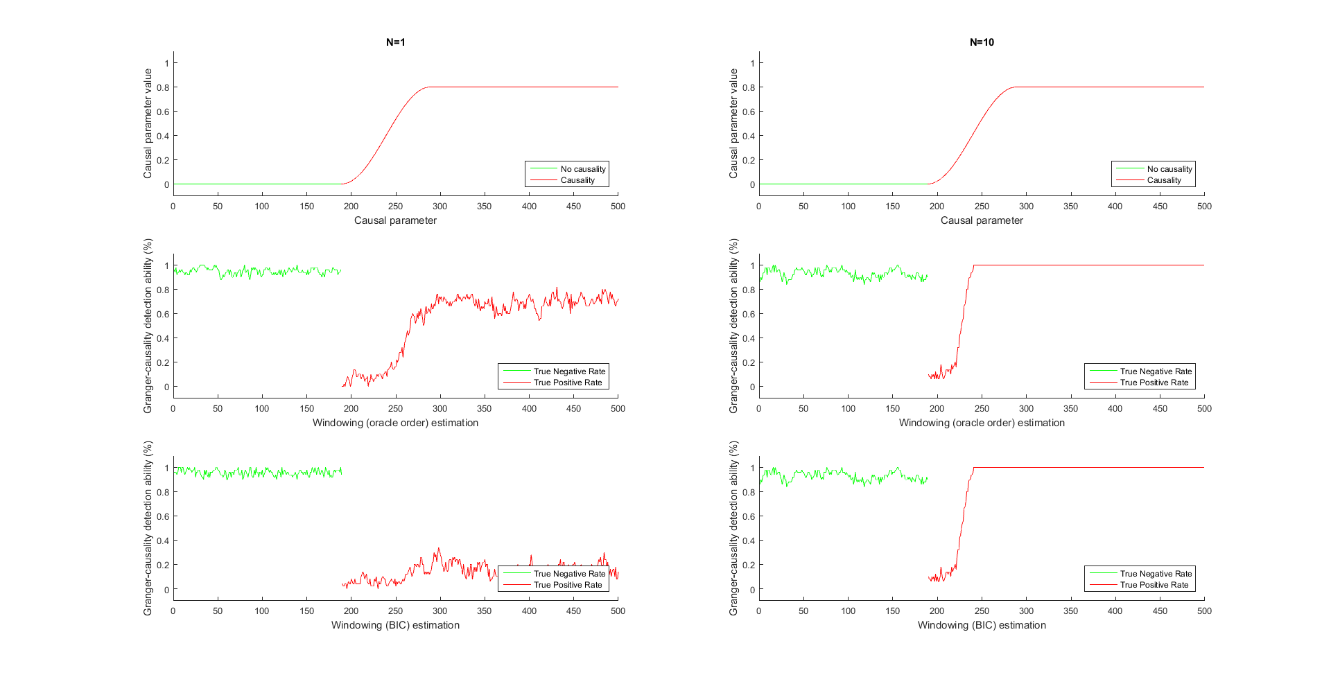
Figure 55: Granger-causality detection ability for a windowing estimation procedure with a model order $2$ and series length $500$ and causal parameter $0.8$.

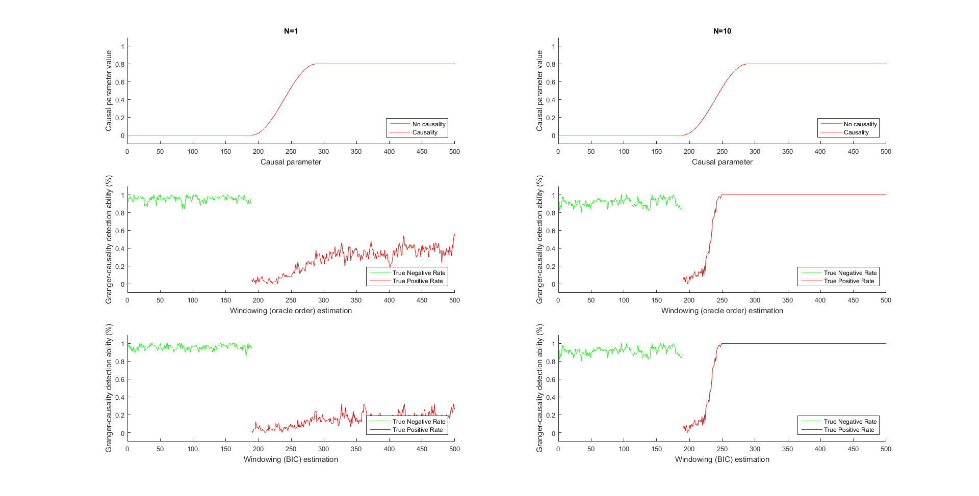
Figure 56: Granger-causality detection ability for a windowing estimation procedure with a model order $4$ and series length $500$ and causal parameter $0.8$.

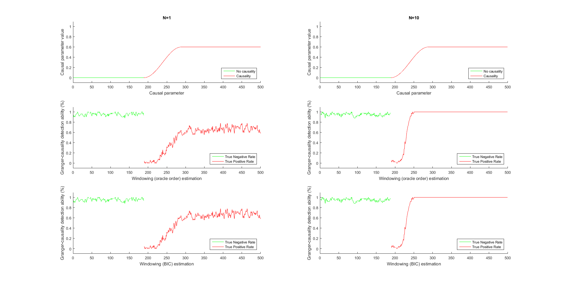
Figure 57: Granger-causality detection ability for a windowing estimation procedure with a model order $1$ and series length $500$ and causal parameter $0.6$.

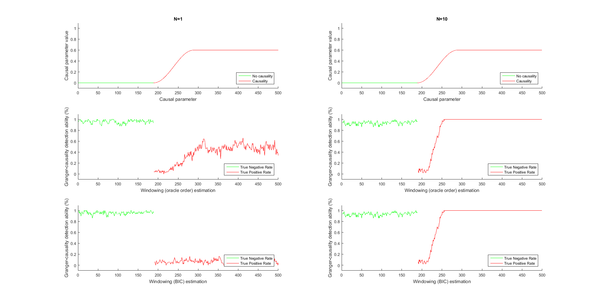
Figure 58: Granger-causality detection ability for a windowing estimation procedure with a model order $2$ and series length $500$ and causal parameter $0.6$.

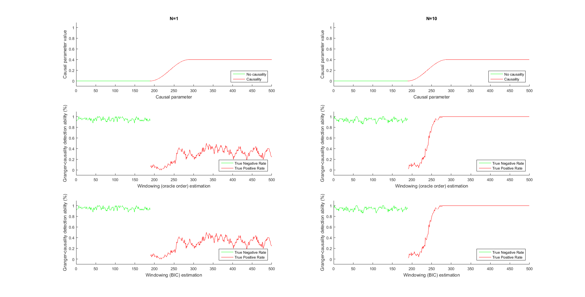
Figure 59: Granger-causality detection ability for a windowing estimation procedure with a model order $1$ and series length $500$ and causal parameter $0.4$.

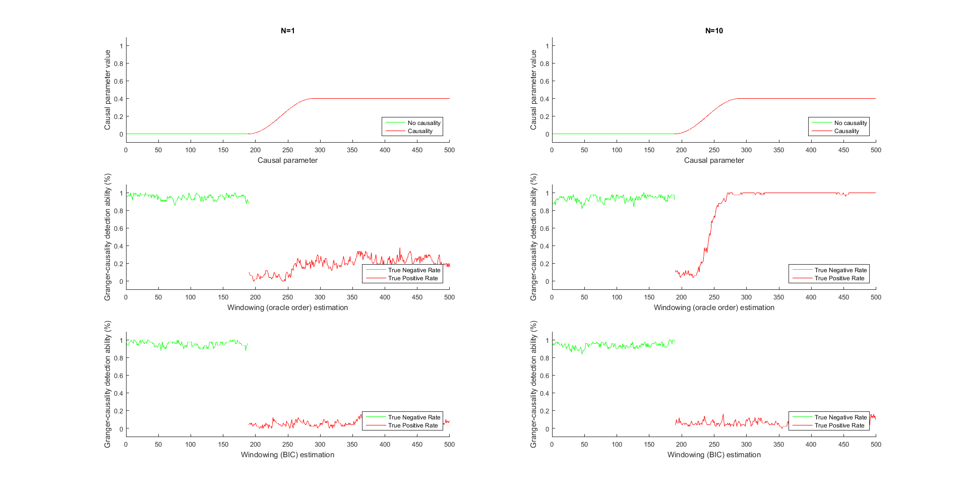
Figure 60: Granger-causality detection ability for a windowing estimation procedure with a model order $2$ and series length $500$ and causal parameter $0.4$.

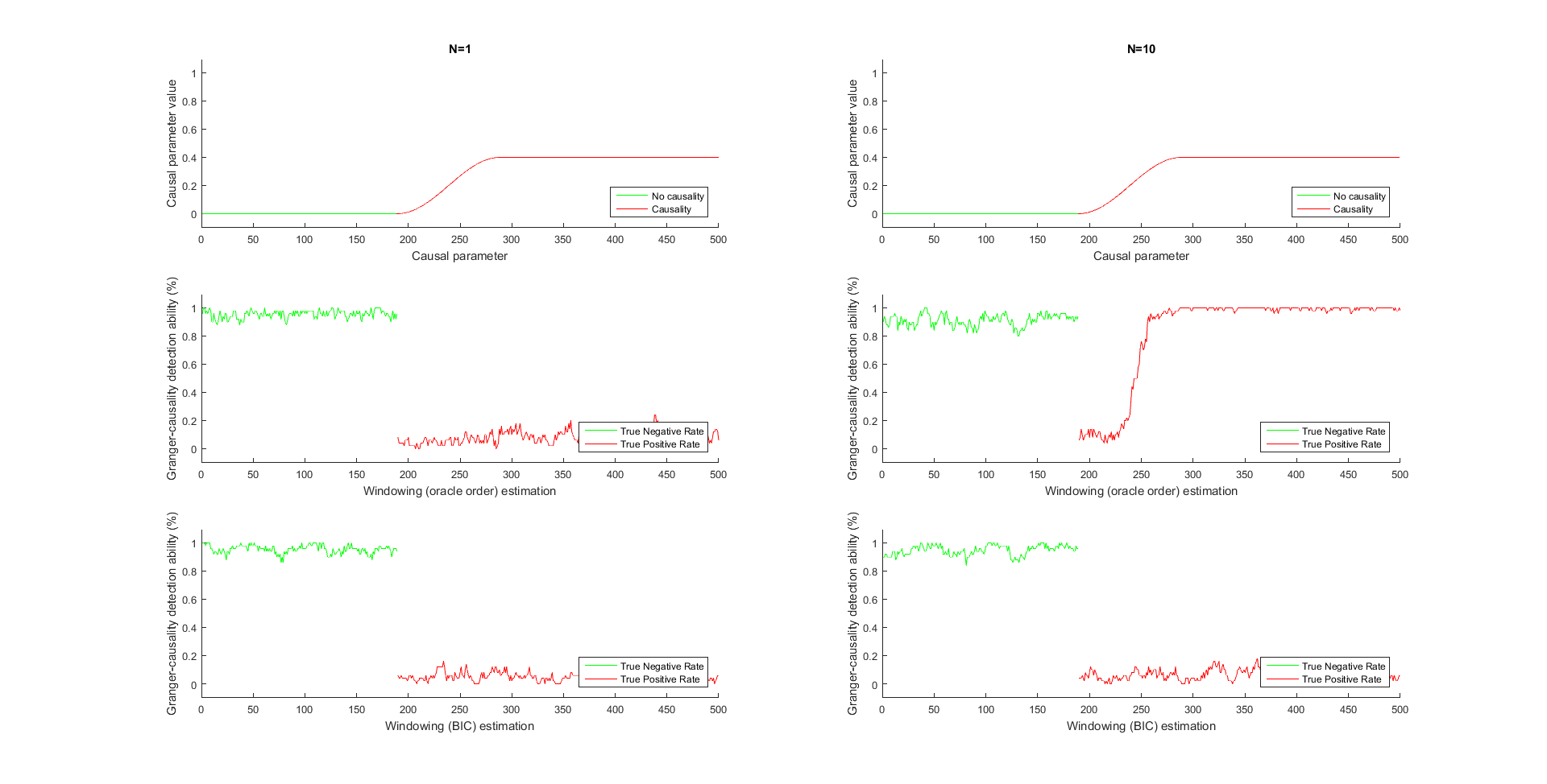
Figure 61: Granger-causality detection ability for a windowing estimation procedure with a model order $4$ and series length $500$ and causal parameter $0.4$.

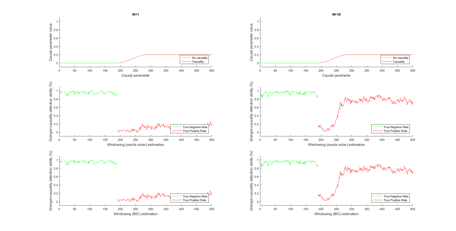
Figure 62: Granger-causality detection ability for a windowing estimation procedure with a model order $1$ and series length $500$ and causal parameter $0.2$.

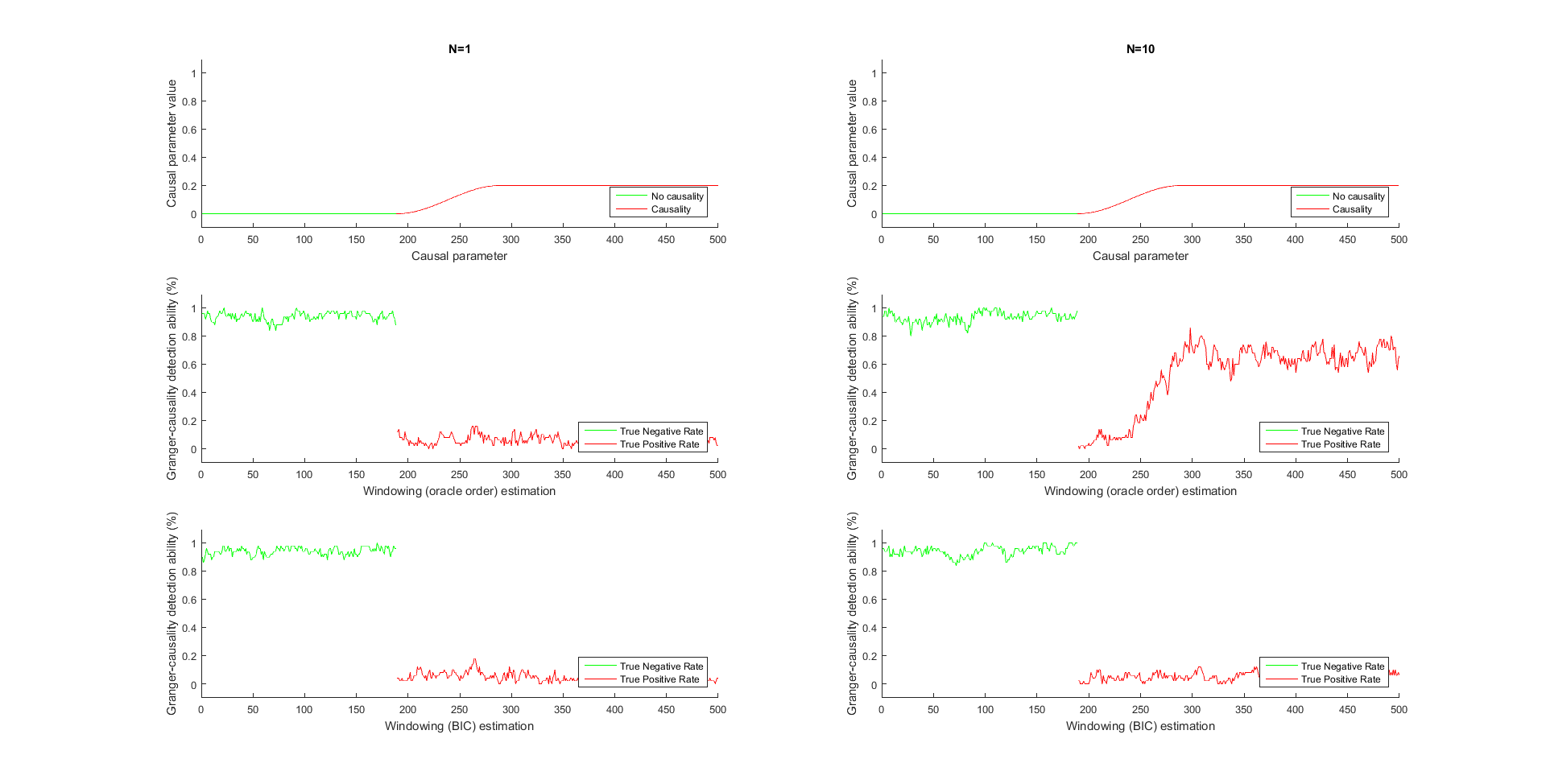
Figure 63: Granger-causality detection ability for a windowing estimation procedure with a model order $2$ and series length $500$ and causal parameter $0.2$.

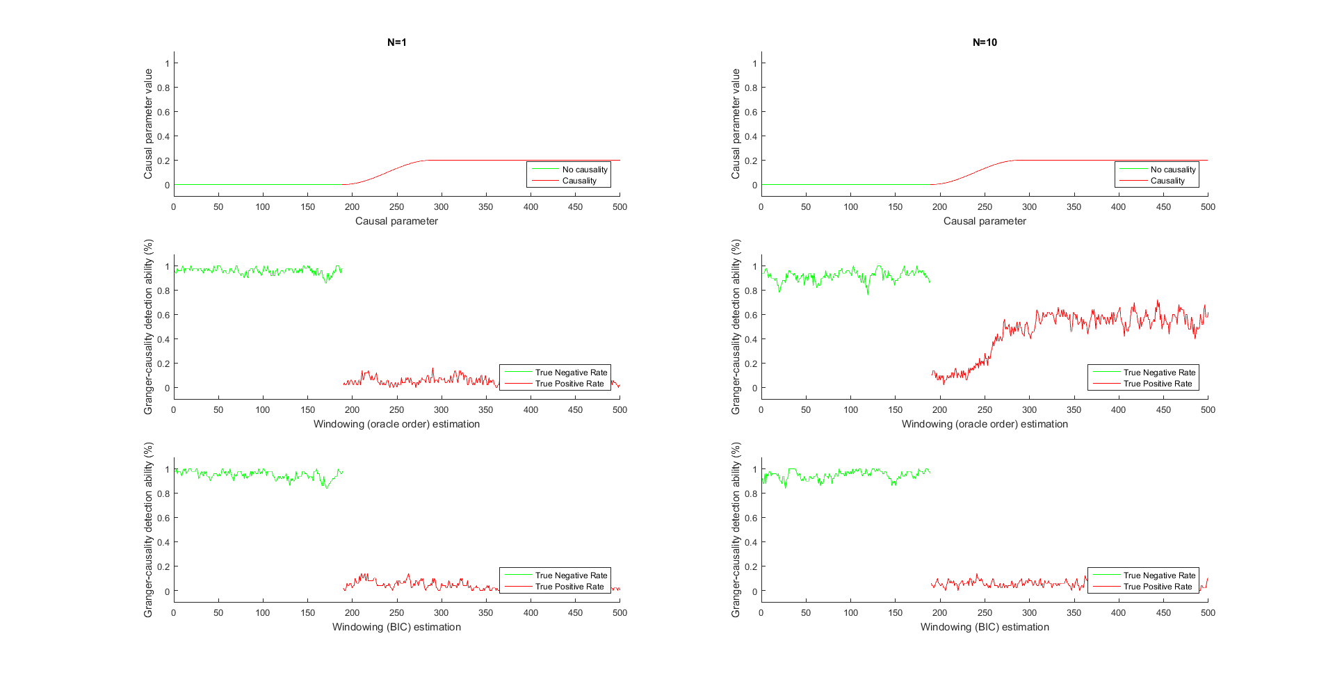
Figure 64: Granger-causality detection ability for a windowing estimation procedure with a model order $4$ and series length $500$ and causal parameter $0.2$.

References

- Arnold et al. [1998] M. Arnold, X. H. R. Milner, H. Witte, R. Bauer, and C. Braun. Adaptive AR modeling of nonstationary time series by means of Kalman filtering. IEEE Transactions on Biomedical Engineering, 45(5):553–562, 1998.
- Attias [1999] H. Attias. Inferring Parameters and Structure of Latent Variable Models by Variational Bayes. In Proceedings of the Fifteenth Conference on Uncertainty in Artificial Intelligence, UAI’99, pages 21–30, San Francisco, 1999. Morgan Kaufmann. ISBN 1-55860-614-9. URL http://dl.acm.org/citation.cfm?id=2073796.2073799.
- Barber and Chiappa [2007] D. Barber and S. Chiappa. Unified Inference for Variational Bayesian Linear Gaussian State-Space Models. In B.Schölkopf, J.C.Platt, and T.Hofmann, editors, Advances in Neural Information Processing Systems 19 (NIPS 2006), pages 81–88. MIT Press, 2007.
- Barnett and Seth [2015] L. Barnett and A. K. Seth. Granger causality for state-space models. Physical Review E, 91(4):040101, 2015. doi: 10.1103/PhysRevE.91.040101.
- Barnett and Seth [2017] L. Barnett and A. K. Seth. Detectability of Granger causality for subsampled continuous-time neurophysiological processes. Journal of Neuroscience Methods, 275:93–121, 2017. ISSN 01650270. doi: 10.1016/j.jneumeth.2016.10.016.
- Beal [2003] M. Beal. Variational Algorithms for Approximate Bayesian Inference. PhD thesis, Gatsby Computational Neuroscience Unit, University College London, London, 2003.
- Box and Tiao [1973] G. E. P. Box and G. C. Tiao. Bayesian Inference in Statistical Analysis. Addison-Wesley, Reading, Massachusetts, 1973.
- Casella and George [1992] G. Casella and E. I. George. Explaining the Gibbs sampler. The American Statistician, 46(3):167–174, 1992.
- Cassidy [2002] W. Cassidy, M.J. Penny. Bayesian nonstationary autoregressive models for biomedical signal analysis. IEEE Transactions on Biomedical Engineering, 49(10):1142–1152, 2002.
- Cekic [2010] S. Cekic. Lien entre activité neuronale des sites cérébraux de l’amygdale et du cortex orbito-frontal en réponse à une prosodie émotionnelle: investigation par la Granger-causalité. Master Thesis, University of Geneva, 2010.
- Cekic [2015] S. Cekic. Time-frequency Granger causality with application to nonstationary brain signals. PhD Thesis, University of Geneva, https://archive-ouverte.unige.ch/unige:78968, 2015.
- Cekic et al. [2018] S. Cekic, D. Grandjean, and O. Renaud. Time, Frequency and Time-Varying Granger-Causality Measures in Neuroscience. Statistics in Medicine, 2018. doi: 10.1002/sim.7621.
- Chen [2005] L. Chen. Vector time-varying autoregressive (TVAR) models and their application to downburst wind speeds. PhD thesis, Texas Tech University, 2005.
- Corduneanu and Bishop [2001] A. Corduneanu and C. M. Bishop. Variational Bayesian model selection for mixture distributions. In Artificial intelligence and Statistics, volume 2001, pages 27–34. Morgan Kaufmann Waltham, MA, 2001.
- Cui et al. [2008] J. Cui, L. Xu, S. L. Bressler, M. Ding, and H. Liang. BSMART: A Matlab/C toolbox for analysis of multichannel neural time series. Neural Networks, 21(8):1094–1104, 2008. doi: 10.1016/j.neunet.2008.05.007.
- Dempster et al. [1977] A. P. Dempster, N. M. Laird, and D. B. Rubin. Maximum Likelihood from Incomplete Data via the EM Algorithm (with Discussion). Journal of the Royal Statistical Society. Series B (Methodological), 39(1):1–38, 1977.
- Ding et al. [2000] M. Ding, S. L. Bressler, W. Yang, and H. Liang. Short-window spectral analysis of cortical event-related potentials by adaptive multivariate autoregressive modeling: data preprocessing, model validation, and variability assessment. Biological Cybernetics, 83(1):35–45, 2000.
- Fox and Roberts [2012] C. W. Fox and S. J. Roberts. A tutorial on variational Bayesian inference. Artificial Intelligence Review, 38(2):85–95, 2012.
- Friston et al. [2007] K. Friston, J. Mattout, N. Trujillo-Barreto, J. Ashburner, and W. Penny. Variational free energy and the Laplace approximation. NeuroImage, 34(1):220–234, 2007. doi: 16/j.neuroimage.2006.08.035.
- Gelman [2006] A. Gelman. Prior distributions for variance parameters in hierarchical models (comment on article by Browne and Draper). Bayesian Analysis, 1(3):515–534, 2006. doi: 10.1214/06-BA117A.
- Ghahramani and Beal [2001] Z. Ghahramani and M. J. Beal. Propagation Algorithms for Variational Bayesian Learning. Advances in Neural Information Processing Systems, 13:507–513, 2001. URL http://citeseer.ist.psu.edu/viewdoc/summary?doi=10.1.1.16.7228.
- Grandjean and Scherer [2008] D. Grandjean and K. R. Scherer. Unpacking the cognitive architecture of emotion processes. Emotion, 8(3):341–351, 2008.
- Grandjean et al. [2005] D. Grandjean, D. Sander, G. Pourtois, S. Schwartz, M. L. Seghier, K. R. Scherer, and P. Vuilleumier. The voices of wrath: brain responses to angry prosody in meaningless speech. Nature Neuroscience, 8(2):145–146, 2005.
- Grandjean et al. [2006] D. Grandjean, T. Bänziger, and K. R. Scherer. Intonation as an interface between language and affect. Progress in brain research, 156:235–247, 2006.
- Granger [1969] C. W. J. Granger. Investigating Causal Relations by Econometric Models and Cross-spectral Methods. Econometrica, 37(3):424–438, 1969. URL http://www.jstor.org/stable/1912791.
- Hamilton [1994] J. D. Hamilton. Time Series Analysis, volume 2. Princeton University Press, 1994.
- Hesse et al. [2003] W. Hesse, E. Möller, M. Arnold, and B. Schack. The use of time-variant EEG Granger causality for inspecting directed interdependencies of neural assemblies. Journal of Neuroscience Methods, 124(1):27–44, 2003. ISSN 0165-0270.
- Huang et al. [2013] A. Huang, M. P. Wand, et al. Simple marginally noninformative prior distributions for covariance matrices. Bayesian Analysis, 8(2):439–452, 2013.
- Kalman [1960] R. E. Kalman. A new approach to linear filtering and prediction problems. Journal of Basic Engineering, 82(1):35–45, 1960.
- Kalman and Bucy [1961] R. E. Kalman and R. S. Bucy. New Results in Linear Filtering and Prediction Theory. Journal of Basic Engineering, 83(1):95–108, 1961. ISSN 0098-2202. doi: 10.1115/1.3658902.
- Kim and Press [1994] H. J. Kim and S. J. Press. Bayesian hypothesis testing of equality of normal covariance matrices, volume 24 of Lecture Notes–Monograph Series, pages 323–330. Institute of Mathematical Statistics, Hayward, CA, 1994. doi: 10.1214/lnms/1215463805.
- Lin et al. [2009] F.-H. Lin, K. Hara, V. Solo, M. Vangel, J. W. Belliveau, S. M. Stufflebeam, and M. S. Hämäläinen. Dynamic Granger-Geweke causality modeling with application to interictal spike propagation. Human Brain Mapping, 30(6):1877–1886, 2009.
- Luessi et al. [2014] M. Luessi, S. D. Babacan, R. Molina, J. R. Booth, and A. K. Katsaggelos. Variational Bayesian causal connectivity analysis for fMRI. Frontiers in Neuroinformatics, 8:45, 2014. doi: 10.3389/fninf.2014.00045.
- Lütkepohl [2005] H. Lütkepohl. New Introduction to Multiple Time Series Analysis. Cambridge University Press, 2005.
- Maris and Oostenveld [2007] E. Maris and R. Oostenveld. Nonparametric statistical testing of EEG- and MEG-data. Journal of Neuroscience Methods, 164(1):177–190, 2007.
- Menictas and Wand [2013] M. Menictas and M. P. Wand. Variational inference for marginal longitudinal semiparametric regression. Stat, 2(1):61–71, 2013.
- Mullen et al. [2010] T. Mullen, A. Delorme, C. Kothe, and S. Makeig. An Electrophysiological Information Flow Toolbox for EEGLAB. Biol. Cybern, 83:35–45, 2010.
- Ormerod and Wand [2010] J. T. Ormerod and M. P. Wand. Explaining Variational Approximations. The American Statistician, 64(2):140–153, 2010. ISSN 0003-1305. doi: 10.1198/tast.2010.09058.
- Ostwald et al. [2014] D. Ostwald, E. Kirilina, L. Starke, and F. Blankenburg. A tutorial on variational Bayes for latent linear stochastic time-series models. Journal of Mathematical Psychology, 60:1–19, 2014.
- Penny [2012] W. D. Penny. Comparing dynamic causal models using AIC, BIC and free energy. NeuroImage, 59(1):319–330, 2012.
- Renaud et al. [2003] O. Renaud, J.-L. Starck, and F. Murtagh. Prediction Based on a Multiscale Decomposition. International Journal of Wavelets, Multiresolution and Information Processing, 1(2):217–232, 2003.
- Roberts and Penny [2002] S. J. Roberts and W. D. Penny. Variational Bayes for generalized autoregressive models. IEEE Transactions on Signal Processing, 50(9):2245–2257, 2002.
- Särkkä [2013] S. Särkkä. Bayesian Filtering and Smoothing. Cambridge University Press, Cambridge, UK, 2013.
- Schlögl [2000] A. Schlögl. The electroencephalogram and the adapdative autoregressive model: theory and applications. PhD thesis, University of Graz, Graz, 2000.
- Schlögl et al. [2000] A. Schlögl, S. Roberts, and G. Pfurtscheller. A criterion for adaptive autoregressive models. In Proceedings of the 22nd IEEE International Conference on Engineering in Medicine and Biology, pages 1581–1582, 2000.
- Seth [2010] A. K. Seth. A MATLAB toolbox for Granger causal connectivity analysis. Journal of Neuroscience Methods, 186(2):262–273, 2010.
- Shumway and Stoffer [1982] R. H. Shumway and D. S. Stoffer. An approach to time series smoothing and forecasting using the EM algorithm. Journal of Time Series Analysis, 3(4):253–264, 1982.
- Solo [2016] V. Solo. State-Space Analysis of Granger-Geweke Causality Measures with Application to fMRI. Neural computation, 28(5):914–949, 2016. ISSN 0899-7667. doi: 10.1162/NECO˙a˙00828.
- Titterington [2004] D. M. Titterington. Bayesian Methods for Neural Networks and Related Models. Statistical Science, 19(1):128–139, 2004. URL http://www.jstor.org/stable/4144378.
- Wand et al. [2011] M. P. Wand, J. T. Ormerod, S. A. Padoan, and R. Fuhrwirth. Mean Field Variational Bayes for Elaborate Distributions. Bayesian Analysis, 6(4):847–900, 2011. URL http://dx.doi.org/10.1214/11-BA631.
- Wang and Titterington [2004] B. Wang and D. M. Titterington. Lack of consistency of mean field and variational Bayes approximations for state space models. Neural Processing Letters, 20(3):151–170, 2004.
- West and Harrison [1997] M. West and P. J. Harrison. Bayesian Forecasting & Dynamic Models. Springer, New York, 1997.
- Wiener [1956] N. Wiener. The Theory of Prediction, chapter 8, pages 165–183. McGraw-Hill, New York, 1956.
- Winn et al. [2005] J. Winn, C. M. Bishop, and T. Jaakkola. Variational Message Passing. Journal of Machine Learning Research, 6(4):661–694, 2005. URL http://search.ebscohost.com/login.aspx?direct=true&db=buh&AN=18003399&site=ehost-live.