Evolution of force networks in dense granular matter close to jamming

Abstract

When dense granular systems are exposed to external forcing, they evolve on the time scale that is typically related to the externally imposed one (shear or compression rate, for example). This evolution could be characterized by observing temporal evolution of contact networks. However, it is not immediately clear whether the force networks, defined on contact networks by considering force interactions between the particles, evolve on a similar time scale. To analyze the evolution of these networks, we carry out discrete element simulations of a system of soft frictional disks exposed to compression that leads to jamming. By using the tools of computational topology, we show that close to jamming transition, the force networks evolve on the time scale which is much faster than the externally imposed one. The presentation will discuss the factors that determine this fast time scale.

1 Introduction

The interaction between particles that build dense granular matter (DGM) is characterized by the presence of a force network, mesoscopic structure that spontaneously form as a granular system is exposed to shear or compression. These networks are crucial for understanding the static and dynamic properties of DGM, and have been recently studied extensively, using the tools that vary from statistical methods peters05 ; tordesillas_pre10 ; tordesillas_bob_pre12 to network type of analysis daniels_pre12 ; herrera_pre11 ; walker_pre12 and application of topological methods arevalo_pre10 ; arevalo_pre13 ; epl12 ; pre13 ; physicaD14 ; pre14 .

Force networks exhibit complicated time dependent structures. Earlier approaches, used to analyze these structures, usually involved rather arbitrary choices of the force thresholds and often depended on ad hoc descriptions of the structures. To avoid these problems we define the force network physicaD14 as a collection of sets $\{X_{\theta}\}_{\theta\in\mathbb{R}}$ such that for $\theta\geq 0$ the set $X_{\theta}$ is the part of the contact network on which the force interactions between the particles exceed the value $\theta$. In the series of papers epl12 ; pre13 ; physicaD14 ; pre14 , we make use of an algebraic topological technique that rigorously describes geometric structures of the sets $\{X_{\theta}\}_{\theta\in\mathbb{R}}$ over all force levels $\theta$. This approach provides a quantitative description of the force networks. Moreover, it allows us to define a concept of distance between force networks, so we can quantitatively compare them.

In pre14 we focused on comparing force networks in simulated granular systems built from soft, possibly inelastic and/or frictional particles exposed to steady slow compression. In that work we found that force networks’ evolution was characterized by large distances between consecutively sampled states of the systems that were approaching jamming transition from below, and the evolution was much smoother for jammed systems. In particular close to jamming transition, we found rather dramatic evolution of the force networks in all considered systems (frictional or not, with elastic or inelastic particles).

The following unexpected findings obtained in pre14 motivate the present peper. Distances between force networks at consecutive states of the system sampled at the rate used in pre14 are comparable to the distances between force networks at the same packing fraction obtained from different realizations, see Figure 1. Sec. 2 provides a brief description of the plotted quantities while more in depth discussion of the figure is presented in Sec. 3. This result suggests that force networks evolve on a time scale that is much faster than the inverse sampling rate and therefore, the main topic of the present paper is the analysis of the system on extremely fast time scales. Furthermore, we discuss how the time scale characterizing evolution of force networks depend on two externally imposed time scales: the slow one imposed by external driving (compression in the case considered here) and the fast one imposed by the temporal discretization used in our simulations. We show that variation of these two scales provides further insight into the mechanisms governing force network evolution.

2 Methods

Here we give a brief overview of the techniques used; the reader is referred to pre14 for more detailed description of the protocol and definitions of various quantities. We consider a square domain in two spatial dimensions exposed to slow compression by the moving walls. The particles are polydisperse, soft, inelastic disks interacting by normal and tangential forces, with the latter ones modeled by Cundall-Strack type of interaction cundall79 . All quantities are expressed using the average particle diameter, $d$, as the length scale, the binary particle collision time $\tau_{c}=\pi\sqrt{d/(2gk_{n})}$ as the time scale, and the average particle mass, $m$, as the mass scale. Here $k_{n}$ (in units of ${mg/d}$) is the spring constant used for modeling (linear) repulsion force between colliding particles, and $g$ is gravity (used only for the purpose of scaling). For the initial configuration, particles ($\approx 2000$) are placed on a square lattice and given random initial velocities. Except if specified differently, the walls move at a uniform inward velocity $v_{c}=2.5\cdot 10^{-5}$. We integrate Newton’s equations of motion for both the translational and rotational degrees of freedom using a $4$th order predictor-corrector method with time step $\delta t={1/50}$.

We use persistent homology edelsbrunner:harer to quantitatively describe the structure of force networks. Briefly, each network is represented by two persistence diagrams that quantify the changes in geometry of the sets $X_{\theta}$ for all force levels $\theta$. The $\beta_{0}$ ($\beta_{1}$) persistence diagram encodes the appearance and disappearance of connected components (loops) by recording all values at which a connected component (loop) appears in a set $X_{\theta}$ and all values of the force level at which the corresponding connected component (loop) disappears. For a rather brief discussion of persistence, we refer the reader to pre14 and for a more in-depth presentation to physicaD14 . There are different types of well defined distances between the persistence diagrams. Each of these distances measures differences between the force levels at which distinct topological features appear and disappear. In particular, the distance between two $\beta_{0}$ persistence diagrams corresponding to different force networks measures differences between the force values at which distinct connected components/clusters are formed and merged together. In a loose sense, this corresponds to measuring differences between the force chains. The results reported in this paper do not depend on the particular choice of the distance and thus, for brevity, we will focus only on the so called Wasserstain distance, $d_{W^{1}}$, between the $\beta_{0}$ persistence diagrams (see physicaD14 for a detailed definition).

3 Results

We start by recalling the results obtained for slow sampling rate of approximately $100$ samples covering the packing fraction range $[0.63,0.9]$. Since the evolution of force networks varies from realization to realization, and the distances between considered states of the system may be rather noisy, we considered the averages over a large number ($20$) of realizations pre14 . Figure 1 shows that the distances between two consecutive states of a given realization are comparable to the distances between two states resulting from different realizations. This suggests that the memory of the system is lost on the time scale faster than the one defined by the slow sampling rate.

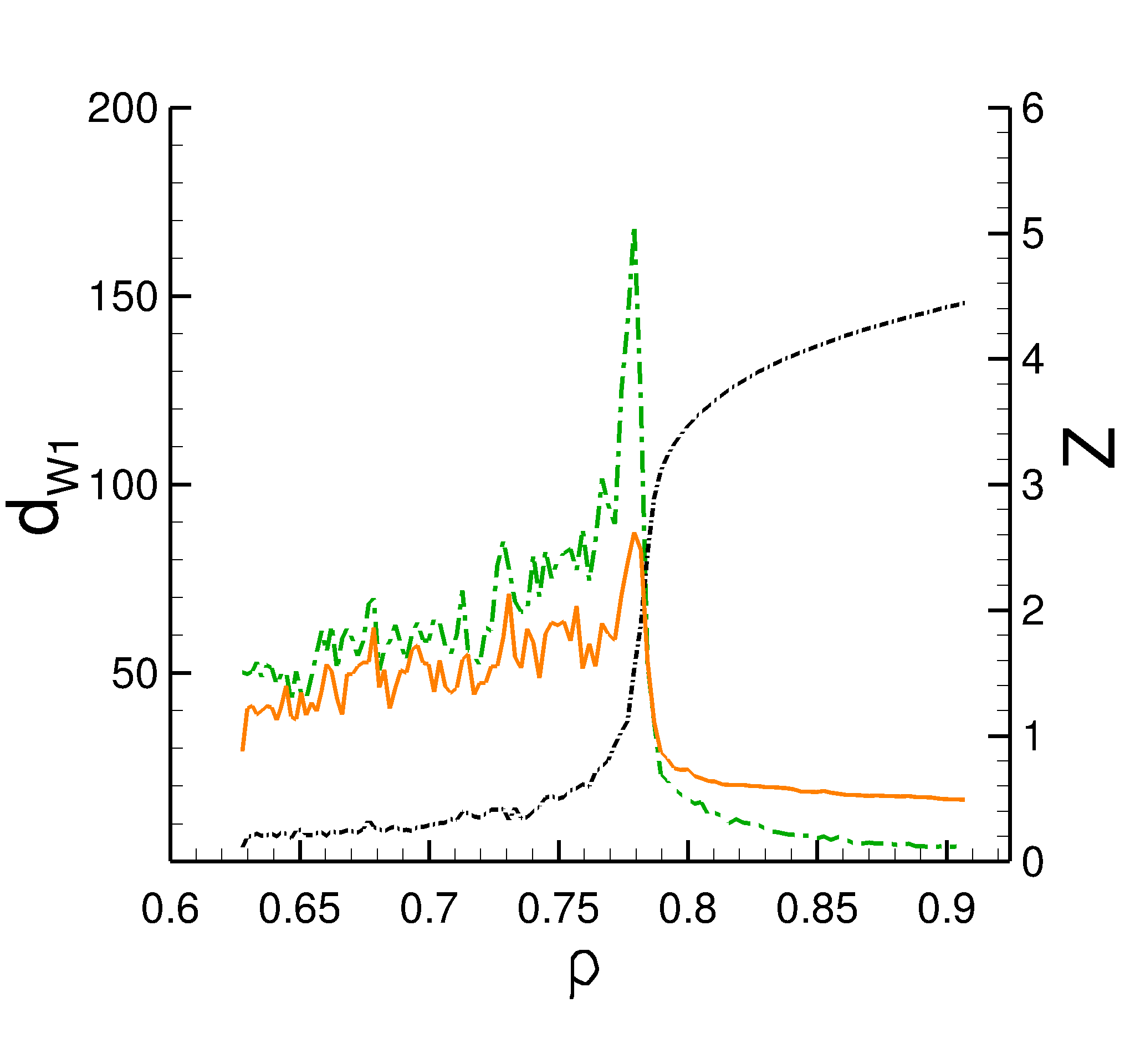
Figure 1: Wasserstein distance, $d_{W^{1}}$, measuring differences between force networks. The dash-dotted (green) line shows the distances of the networks averaged over $20$ realization and the solid (orange) line shows the distances between different realizations. The dotted (black) line shows the number of contacts, $Z$; the rapid rise is a sign of jamming transition.

To proceed, we consider much faster sampling rates. We also focus on presenting and analyzing the results from a single realization, since averaging the results over realizations obscures part of the information about force network evolution in a given system. Figure 2 shows $d_{W^{1}}$ distance for four sampling rates $r_{1},r_{10},r_{100}$ and $r_{1000}$; here the index of a rate corresponds to the number of computational steps of duration $\delta t$ between two consecutive sample points. The difference in the packing fraction, $\rho$, between two consecutive states sampled at the rate $r_{i}$ is $\Delta\rho=i\cdot\delta\rho$ where $\delta\rho\approx 4\cdot 10^{-8}$ is the change of $\rho$ during one computational step. Note that $r_{1}$ corresponds to the fastest possible sampling rate, at which the state of the system is recorded at every time step. First, we note that, as expected, for faster sampling rates, there is a large number of points such that the distance is very small, suggesting that the force networks do not evolve much during a significant portion of the data shown. However, contrary to expectations, there is an increase of the peaks’ sizes as the sampling rate is increased from $r_{1000}$ to $r_{100}$ and $r_{10}$, followed by a gentle decrease as the rate is increased from $r_{10}$ to $r_{1}$. This essentially means that one needs to sample at the rate comparable to $r_{10}$ (at which the peaks in $d_{W^{1}}$ distance are the largest) to capture the corresponding large events present in networks’ evolution. In turn, this implies that large changes between the force networks occur on the time scales shorter than $\tau_{c}$ (capturing the system evolution with the sampling rate given by $1/\tau_{c}$ would correspond to $r_{50}$).

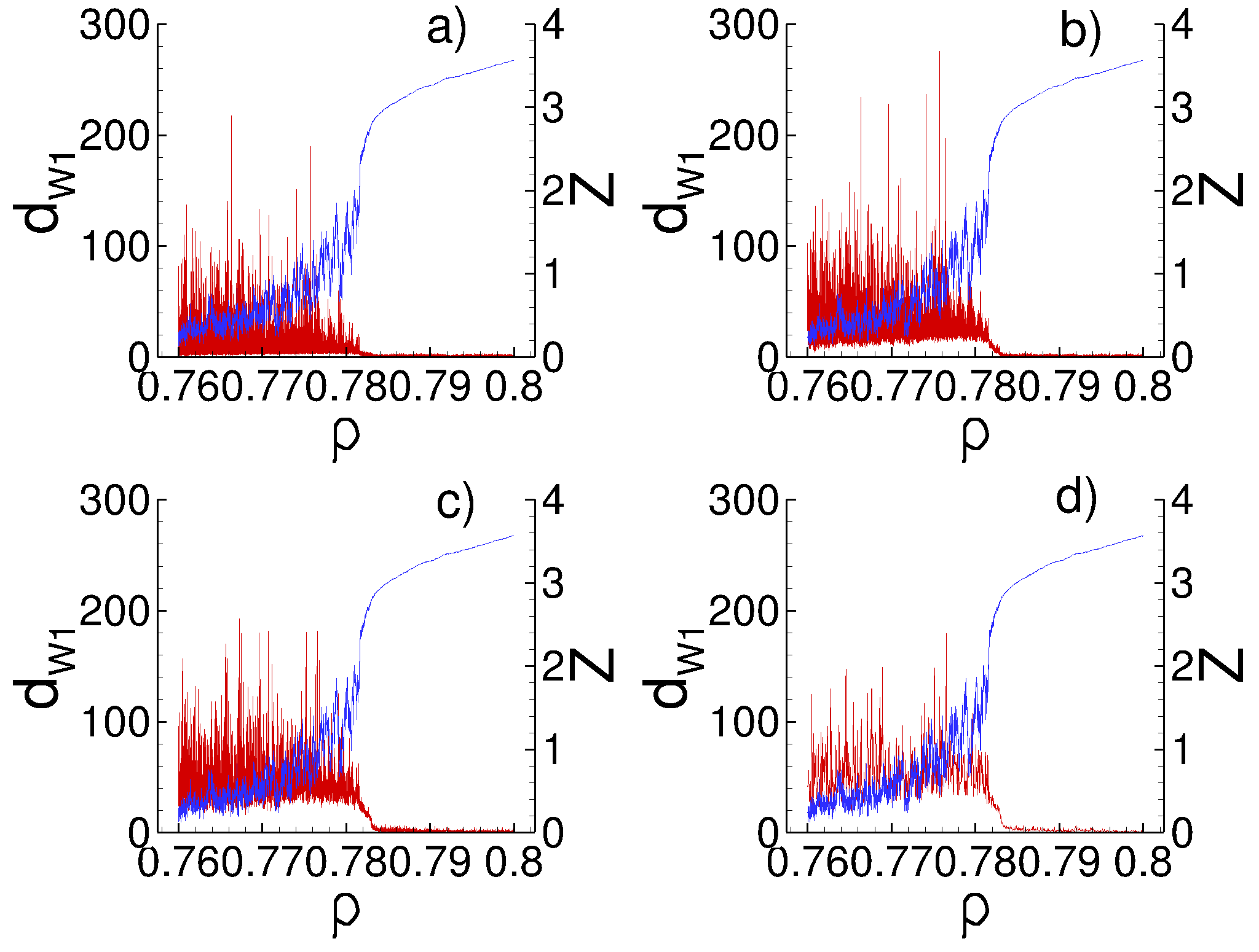
Figure 2: Wasserstein distance $d_{W^{1}}$ (red) between $\beta_{0}$ persistence diagrams computed for different sampling rates: a) $r_{1}$ b) $r_{10}$, c) $r_{100}$ and d) $r_{1000}$. The number of contacts between particles, $Z$ is shown in blue.

The number of data points shown in Fig. 2 is large; e.g., Fig. 2a shows about $10^{6}$ data points. Since it is impractical to work with such a large number of data points, we proceed by carrying out a running average of the data shown in Fig. 2, and then proceed with considering a subset of the data extracted from the region very close to the jamming transition (that occurs at $\rho\approx 0.78$ for the present system). Figure 3 shows the running averages for $d_{W^{1}}$ distance. The averaging interval is given by $10^{4}\delta\rho\approx 4\cdot 10^{-4}$. This averaging interval corresponds to the averaging time of about $200\tau_{c}$ which for a common granular system may range between a $\mu$sec and a msec. The actual number of points used for computing varies from $10^{4}$ for the fastest sampling rate $r_{1}$ to $10$ for the slowest sampling rate $r_{1000}$.

Before jamming transition a typical distance between consecutive states grows as the sampling rate decreases, but at a rate that is typically much slower than expected. Note that the consecutive sampling rates differ by one order of magnitude. However, the differences between averaged distances is one order of magnitude only for the sampling rates $r_{1}$ and $r_{10}$ and becomes significantly smaller for slower sampling; the results are actually overlapping for $r_{100}$ and $r_{1000}$. This finding suggests, consistently with the results shown in Fig. 2, that the time scale on which force networks evolve is comparable to $\tau_{c}$ or even shorter.

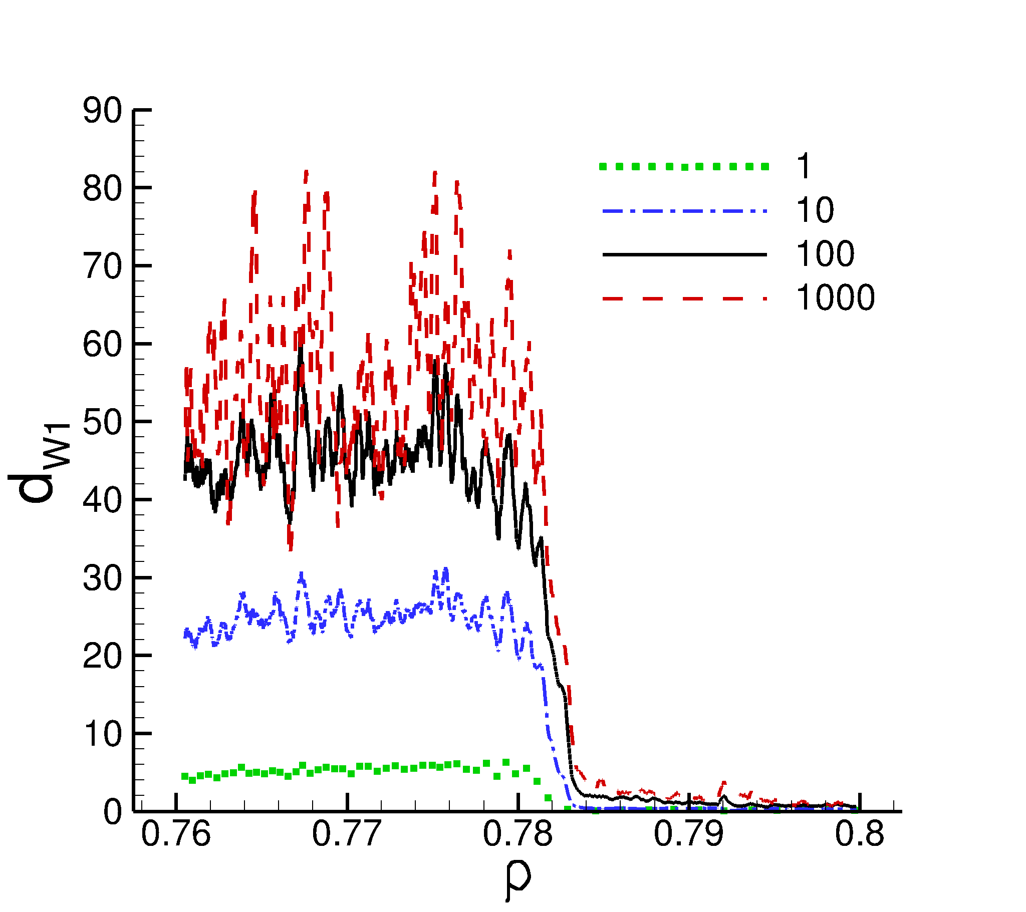
Figure 3: Running average of $d_{W^{1}}$-distances over $10^{4}\delta\rho$. The curves correspond to the sampling rate used to compute the distances shown in Fig. 2.

The fast time scale on which force networks evolve raises new questions. Recall that $\delta t$ is the time interval needed for information about possible interactions to travel across a particle and hence $\delta t$ is related to the speed of sound, $v_{s}$, in the material. In particular, the approximate speed of sound, determined by the numerical time step, is given (in physical units) by $d/({\delta t\tau_{c}})$, and therefore, information about the features present in force networks that evolve on the time scale given by $\delta t$ essentially propagates by the speed of sound. Thus, it is natural to ask whether the results may be influenced by $\delta t$.

Figure 4 shows an influence of decreasing $\delta t$ on $d_{W^{1}}$ distance in a small interval based at $\rho\approx 0.78$. Consequences of decreasing the $\delta t$ are two fold. On one hand, as $\delta t$ decreases, on average $d_{W^{1}}$ decreases (the number of points at which $d_{W^{1}}$ is very small increases as $\delta t$ decreases). On the other hand, we notice that the peaks’ heights do not necessarily decrease with $\delta t$, and more importantly, the peaks still relax on the scale corresponding to $\delta t$: for smaller $\delta t$’s, the peaks relax faster (see the insets in Fig. 4). This finding is consistent with the general discussion above regarding the relevance of the speed of sound, and is showing clearly that in the considered system the force networks evolve on the time scale determined by the speed of sound in the material.

Another question to ask is related to the influence of the compression speed, $v_{c}$, which defines a slow time scale in the problem. As $v_{c}$ is reduced, one may expect that the distance between the consecutive states of the system becomes smaller. As we show next, such trend is indeed observed in our results.

Figure 5 shows $d_{W^{1}}$ distance at the same $\rho$ as in Fig. 4, but now for four (decreasing) $v_{c}$’s. We see that, indeed, on average $d_{W^{1}}$ decreases as $v_{c}$ is decreased, meaning that there are many $\delta t$ intervals when the force networks essentially do not evolve. However, the height of the peaks does not necessarily decrease with $v_{c}$; we even find examples of larger peaks for slower compression. This finding can be understood by realizing that as the system is compressed slower, the particles have higher chance to rearrange, leading in some cases to large changes in the force network and increased distances between the consecutive states.

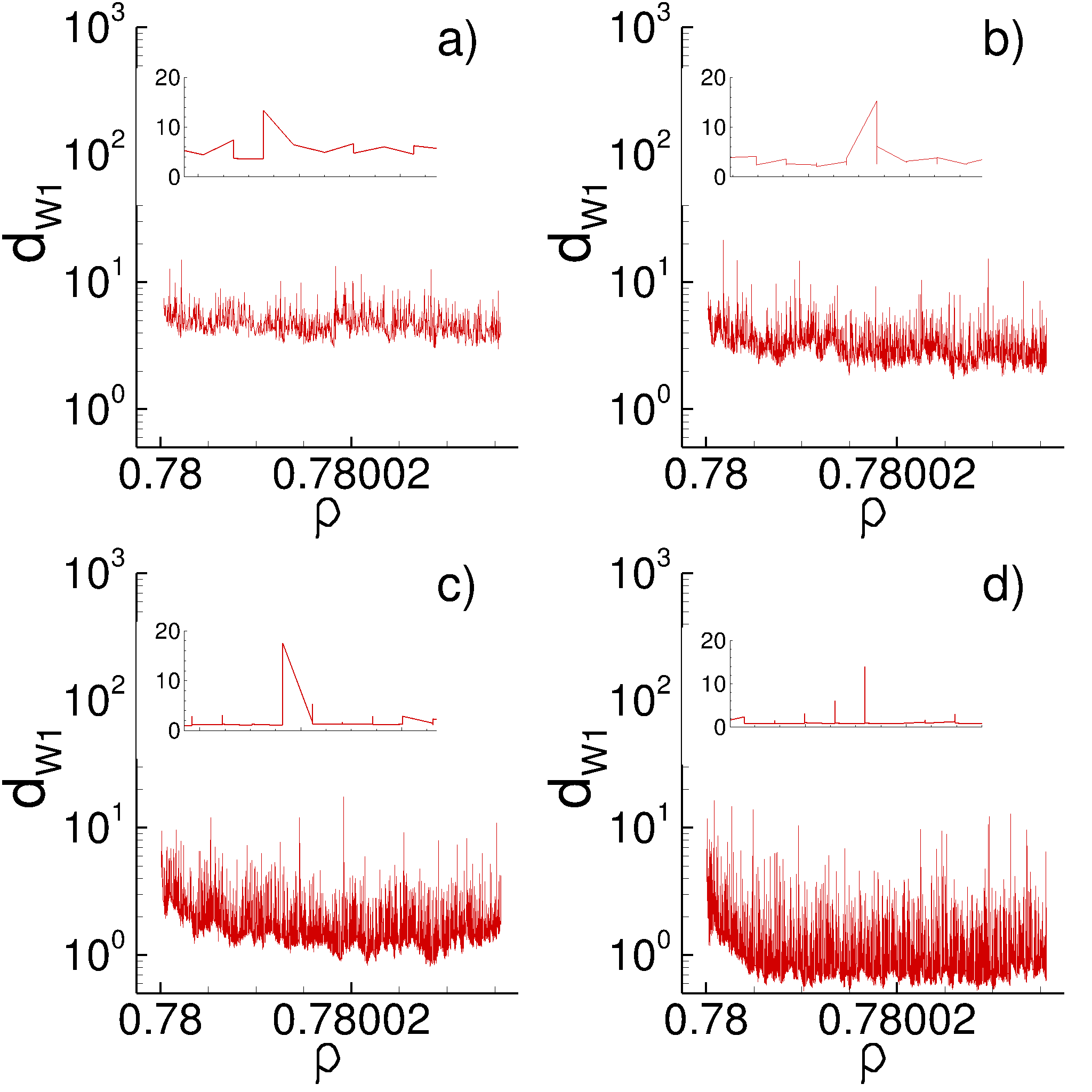
Figure 4: $d_{W^{1}}$ distance between $\beta_{0}$ persistence diagrams corresponding to the consecutive force networks (one computational time step apart) for $\rho\approx 0.78$ as $\delta t$ is reduced, with the part a) using the reference value $\delta t=1/50$, and the parts b), c), d) using $\delta t/2$, $\delta t/4$, and $\delta t/8$, respectively. The insets show the distances for few consecutive time steps, with the shown range of $5\times 10^{-7}$. The compression speed, $v_{c}$, is kept fixed.

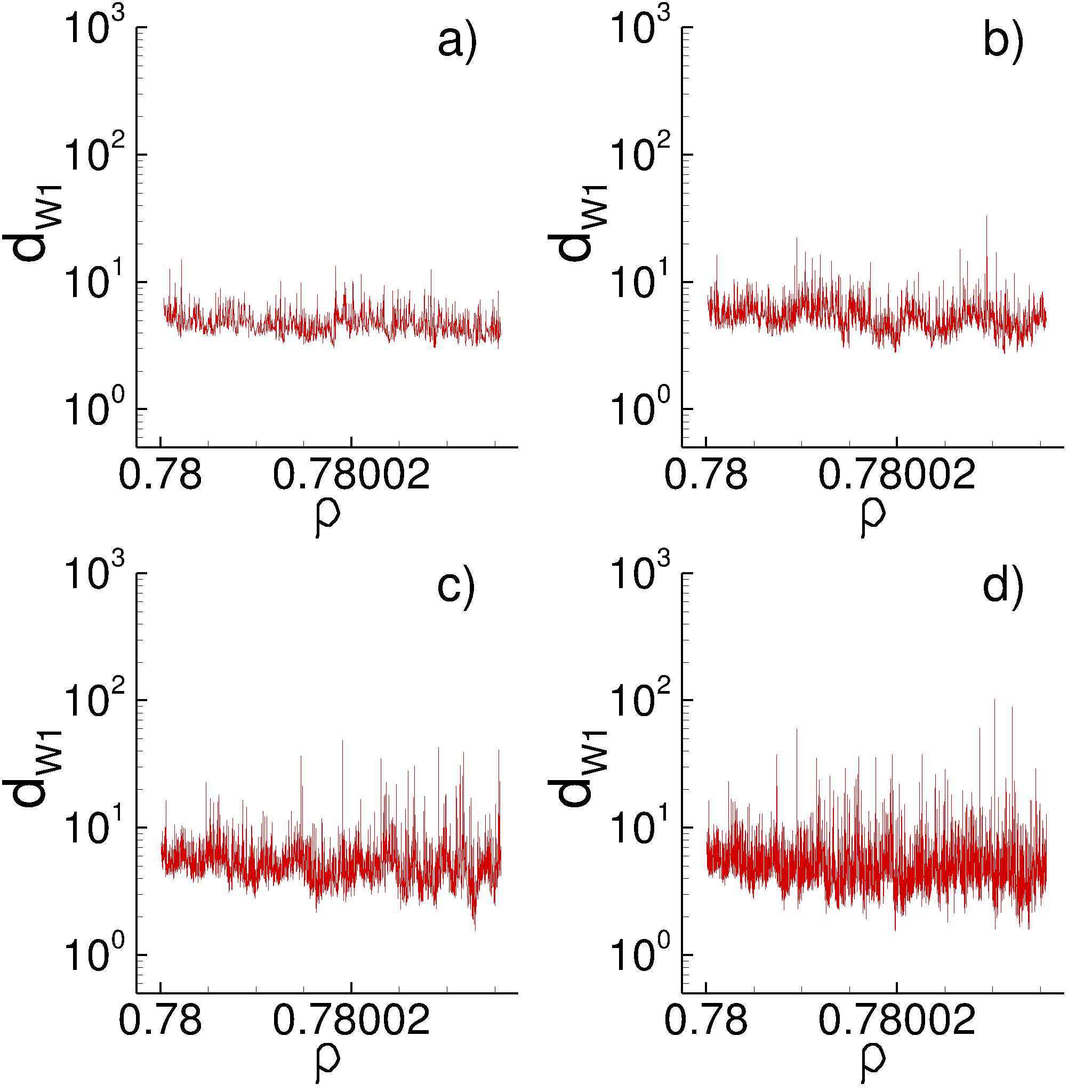
Figure 5: $d_{W^{1}}$ distance between $\beta_{0}$ persistence diagrams corresponding to the consecutive force networks (one $\delta t$ apart) for $\rho\approx 0.78$ as the compression speed is reduced, with the part a) using the reference value, $v_{c}$, and the parts b), c), and d) using $v_{c}/2$, $v_{c}/4$ and $v_{c}/8$, respectively. $\delta t$ is kept fixed.

4 Conclusions

The force networks are found to evolve on the time scale that is much faster than the one introduced by externally imposed driving. As a consequence, an analysis of dynamics of force networks based on slow sampling rates may provide incomplete information about the networks’ evolution, since slow sampling may miss large events that occur on faster time scales. In particular, we find that the time scale on which evolution occurs is specified by $d/v_{s}$, where $d$ is a typical particle diameter and $v_{s}$ the speed of sound in the material. It will be of interest to see to which degree such behavior can be seen in experimental systems. Furthermore, it should be noted that in the present work we focus on the systems very close to jamming transition; it remains to be seen whether such fast evolution as uncovered here may be seen further away from jamming, and/or for different type of external forcing.

The reported results rely on the use of computational homology that allows us to quantify the differences between force networks as a granular system evolves. One particular strength of the computational homology approach is that it is system-independent and can be applied to any system, independently of the physical properties of the considered system, such as the type of interaction between the particles, or the number of dimensions of the physical space in which they live. Therefore, natural next step will be to consider particulate systems characterized by different physical properties (friction, polydispersity, cohesion, shape) or different geometry (2D versus 3D). Furthermore, the approach can be as well applied to experimental systems, such as those built from photoelastic particles, where detailed information about the force networks is available. Further analyses of such systems will be the subject of our future works.

References

- (1) J. Peters, M. Muthuswamy, J. Wibowo, A. Tordesillas, Phys. Rev. E 72, 041307 (2005)
- (2) A. Tordesillas, D.M. Walker, Q. Lin, Phys. Rev. E 81, 011302 (2010)
- (3) A. Tordesillas, D.M. Walker, G. Froyland, J. Zhang, R. Behringer, Phys. Rev. E 86, 011306 (2012)
- (4) D.S. Bassett, E.T. Owens, K.E. Daniels, M.A. Porter, Phys. Rev. E 86, 041306 (2012)
- (5) M. Herrera, S. McCarthy, S. Sotterbeck, E. Cephas, W. Losert, M. Girvan, Phys. Rev. E 83, 061303 (2011)
- (6) D. Walker, A. Tordesillas, Phys. Rev. E 85, 011304 (2012)
- (7) R. Arévalo, I. Zuriguel, D. Maza, Phys. Rev. E 81, 041302 (2010)
- (8) R. Arévalo, L.A. Pugnaloni, I. Zuriguel, D. Maza, Phys. Rev. E 87, 022203 (2013)
- (9) L. Kondic, A. Goullet, C. O’Hern, M. Kramár, K. Mischaikow, R. Behringer, Europhys. Lett. 97, 54001 (2012)
- (10) M. Kramár, A. Goullet, L. Kondic, K. Mischaikow, Phys. Rev. E 87, 042207 (2013)
- (11) M. Kramár, A. Goullet, L. Kondic, K. Mischaikow, Physica D 283, 37 (2014)
- (12) M. Kramár, A. Goullet, L. Kondic, K. Mischaikow, Phys. Rev. E 90, 052203 (2014)
- (13) P.A. Cundall, O.D.L. Strack, Géotechnique 29, 47 (1979)
- (14) H. Edelsbrunner, J.L. Harer, Computational topology (AMS, Providence, RI, 2010)