An optimal FFT-based anisotropic power spectrum estimator

Abstract

Measurements of line-of-sight dependent clustering via the galaxy power spectrum’s multipole moments constitute a powerful tool for testing theoretical models in large-scale structure. Recent work shows that this measurement, including a moving line-of-sight, can be accelerated using Fast Fourier Transforms (FFTs) by decomposing the Legendre polynomials into products of Cartesian vectors. Here, we present a faster, optimal means of using FFTs for this measurement. We avoid redundancy present in the Cartesian decomposition by using a spherical harmonic decomposition of the Legendre polynomials. Consequently, our method is substantially faster: a given multipole of order $\ell$ requires only $2\ell+1$ FFTs rather than the $(\ell+1)(\ell+2)/2$ FFTs of the Cartesian approach. For the hexadecapole ($\ell=4$), this translates to $40\%$ fewer FFTs, with increased savings for higher $\ell$. The reduction in wall-clock time enables the calculation of finely-binned wedges in $P(k,\mu)$, obtained by computing multipoles up to a large $\ell_{\rm max}$ and combining them. This transformation has a number of advantages. We demonstrate that by using non-uniform bins in $\mu$, we can isolate plane-of-sky (angular) systematics to a narrow bin at $\mu\simeq 0$ while eliminating the contamination from all other bins. We also show that the covariance matrix of clustering wedges binned uniformly in $\mu$ becomes ill-conditioned when combining multipoles up to large values of $\ell_{\rm max}$, but that the problem can be avoided with non-uniform binning. As an example, we present results using $\ell_{\rm max}=16$, for which our procedure requires a factor of 3.4 fewer FFTs than the Cartesian method, while removing the first $\mu$ bin leads only to a 7% increase in statistical error on $f\sigma_{8}$, as compared to a 54% increase with $\ell_{\rm max}=4$.

1 Introduction

The clustering of galaxies on the largest scales contains a significant amount of cosmological information. The Baryon Acoustic Oscillation (BAO) feature on scales of $\sim 100\;{\rm Mpc}/h$ can be used as a standard ruler to gauge the Universe’s expansion history and infer properties of dark energy (e.g., [1, 2]). First detected in the 2-point correlation function (2PCF) by [3, 4] and more recently in the 3-point function (3PCF) by [5], the BAO signal has provided percent-level measurements of the Hubble parameter $H(z)$ and angular diameter distance $D_{a}(z)$ [6]. These analyses have measured both the characteristic BAO peak in configuration space [7, 8] and the analogous wiggles in Fourier space [9, 10]. Beyond the BAO, and on even larger scales, these clustering statistics also contain signatures of primordial non-Gaussianity, the deviation from Gaussian Random Field initial conditions in the early Universe [11, 12].

Additional information can be extracted from these statistics by measuring the broadband clustering as a function of the angle to the line-of-sight (LOS). Although the underlying distribution of galaxies is assumed to be homogeneous and isotropic, observational effects such as the Alcock-Paczynski (AP; [13]) effect and redshift-space distortions (RSD; [14]) introduce anisotropy into the measured clustering when a fiducial distance-redshift relation is used to translate redshifts into comoving coordinates. In particular, anisotropy around the line-of-sight is introduced by RSD because an object’s redshift, used to infer the LOS coordinate, is sensitive to its peculiar velocity. Because this velocity is sourced by the large-scale gravity field, RSD measurements allow constraints on the growth rate of structure and can provide tests of General Relativity (e.g., [15]). For galaxy pairs, RSD depend on the angle cosine $\mu$ between the pair separation $\vec{s}$ and the line-of-sight $\hat{n}$. The clustering is typically measured as multipole moments of the 2-point correlation function, which gives the excess of pairs above random, or of the power spectrum, its Fourier space analog. The Legendre polynomials form a complete basis and are equivalent to expanding in powers of $\mu$. Parity demands that only even multipoles are non-zero. In linear theory, RSD generate only $\ell=0,2,$ and $4$ moments of the anisotropic power spectrum [14] or correlation function [16].

For wide-field galaxy surveys, only angle-averaged clustering, i.e., the monopole, can be measured accurately under the assumption of a single LOS to the entire survey. Under this assumption, it is straightforward to measure the clustering using a Fast Fourier Transform (FFT). What is more challenging is to define a clustering estimator for the higher-order multipoles that uses a line-of-sight that rotates to follow each galaxy pair’s spatial or Fourier-space separation. Including the observer as a third vertex, the galaxy pair maps to a triangle, and more accurate line-of-sight choices are the angle bisector of this triangle or the vector from the observer to the separation midpoint. Less accurate but still better than a single LOS is taking the LOS to be the vector from observer to a single pair member, as first used in [17, 18]. This latter method, often referred to as the local plane-parallel approximation, differs from angle bisector and midpoint methods at $\mathcal{O}(\theta^{2})$, where $\theta$ is the angle the pair subtends; bisector and midpoint methods also differ from each other at $\mathcal{O}(\theta^{2})$ [19]. For the current generation of surveys, these wide-angle effects are not a significant source of error [20, 21] but could become important for future surveys, especially for studies which focus primarily on large-scales, i.e., primordial non-Gaussianity analyses. To address this, slight generalizations of the local plane parallel estimates for the multipoles can be combined to form the midpoint and bisector-based estimates [19].

Recently, [22] and [23] showed that by using products of Cartesian coordinates as building blocks for the Legendre polynomials, one could evaluate the local plane-parallel method of [17] using FFTs, providing an enormous speed-up over the summation-based estimator. Around the same time, [24] demonstrated that FFTs could also be used for the anisotropic 2PCF by exploiting the spherical harmonic addition theorem to decompose the Legendre polynomials into spherical harmonics. In this work, we show that this spherical harmonic approach can also be used for the power spectrum multipoles. Importantly, the spherical harmonics are orthogonal to each other, whereas the Cartesian vectors used by [22, 23] are not. Thus, the [22, 23] implementation involves redundancy, requiring $(\ell+1)(\ell+2)/2=\mathcal{O}(\ell^{2})$ FFTs per multipole rather than the $2\ell+1=\mathcal{O}(\ell)$ FFTs needed by our method. We emphasize that our algorithm scales linearly with $\ell$ whereas these previous works scaled with its square.

The additional speed-up provided by our implementation is not only useful for computing higher-order multipoles more quickly but also for the processing of a large number of mock catalogs for estimating covariance matrices. For example, the covariance matrix estimation of [6] required evaluating clustering statistics for 3 separate redshift bins and 1000 mock catalogs. Furthermore, the calculation of higher-order multipoles is also useful for analyzing the clustering in wedges of $\mu$ [25, 26]. While there is little measurable signal in multipoles above the $\ell=4$ hexadecapole, we show that the measurement of multipoles up to a large $\ell_{\rm max}$ allows the use of narrow $\mu$ bins. It also reduces the correlations between separate $\mu$ bins, allowing for easier theoretical modeling of the covariance of the clustering estimator. The use of narrow $\mu$ wedges becomes advantageous when measuring clustering contaminated by systematics in the plane of the sky, as is often the case for galaxy surveys, i.e., [27]. Such a transverse systematic will contaminate all multipoles, but we demonstrate that the contamination can be effectively isolated to a narrow bin around $\mu\simeq 0$ when using wedges, with the width of the $\mu\simeq 0$ bin scaling as $(\ell_{\rm max}/2+1)^{-1}$. Non-uniform binning in $\mu$ can be chosen such that any artifacts of the systematic are eliminated for all bins beyond the first $\mu\simeq 0$ bin.

The paper is laid out as follows. In §2.1, we first present the improved estimator of the power spectrum multipoles using a spherical harmonic expansion and demonstrate that it significantly outperforms the Cartesian decomposition method. This enables us to efficiently measure higher-order multipoles and then transform them into power spectrum wedges as shown in §2.2. We then discuss our implementation of the estimators in the publicly available large-scale structure analysis software nbodykit in §2.3. In §3, we develop a simple model for a systematic signal in the transverse ($\mu=0$) direction and present a simple method to mitigate the contamination with a non-uniform binning scheme. We discuss the impact of survey window function on this method in §3.3. We show in §4.1 that the higher multipoles de-correlate the wedges even though they do not add additional signal. This means that one can reduce the information loss due to removal of the localized contamination by measuring more multipoles (§4.2). Finally, we conclude in §5.

2 Estimators

2.1 Multipoles

We begin by defining the weighted galaxy density field [28],

$$F(\mathbf{r})=\frac{w(\mathbf{r})}{I^{1/2}}\left[n(\mathbf{r})-\alpha n_{s}(\mathbf{r})\right],$$ (2.1)

where $n$ and $n_{s}$ are the observed number density field for the galaxy catalog and synthetic catalog of random objects, respectively. The random catalog defines the expected mean density of the survey and also accounts for the angular mask and radial selection function. It contains no cosmological clustering signal. We allow for a general weighting scheme $w(\mathbf{r})$. The factor $\alpha$ normalizes the synthetic catalog to the number density of the galaxies. The field $F(\mathbf{r})$ is normalized by the factor of $I$, defined as $I\equiv\int d\mathbf{r}\;w^{2}\bar{n}^{2}(\mathbf{r})$. The estimator for the multipole moments of the power spectrum is [28, 17]

$$\widehat{P}_{\ell}(k)=\frac{2\ell+1}{I}\int\frac{d\Omega_{k}}{4\pi}\left[\int\mathrm{d}\mathbf{r}_{1}\int\mathrm{d}\mathbf{r}_{2}\ F(\mathbf{r}_{1})F(\mathbf{r}_{2})e^{i\mathbf{k}\cdot(\mathbf{r}_{1}-\mathbf{r}_{2})}\mathcal{L}_{\ell}(\mathbf{\hat{k}}\cdot\mathbf{\hat{r}}_{h})-P_{\ell}^{\rm noise}(\mathbf{k})\right],$$ (2.2)

where $\Omega_{k}$ represents the solid angle in Fourier space, $\mathbf{r}_{h}\equiv(\mathbf{r}_{1}+\mathbf{r}_{2})/2$ is the line-of-sight to the mid-point of the pair of objects, and $\mathcal{L}_{\ell}$ is the Legendre polynomial of order $\ell$. The shot noise $P_{\ell}^{\rm noise}$ is

$$P_{\ell}^{\rm noise}(\mathbf{k})=(1+\alpha)\int\mathrm{d}\mathbf{r}\ \bar{n}(\mathbf{r})w^{2}(\mathbf{r})\mathcal{L}_{\ell}(\mathbf{\hat{k}}\cdot\mathbf{\hat{r}}),$$ (2.3)

and we assume that $P_{\ell}^{\rm noise}=0$ for $\ell>0$, as it is negligible relative to $\widehat{P}_{\ell}$. We then approximate the line-of-sight to the pair of objects with the line-of-sight to a single pair member, as $\mathcal{L}_{\ell}(\mathbf{\hat{k}}\cdot\mathbf{\hat{r}}_{h})\simeq\mathcal{L}_{\ell}(\mathbf{\hat{k}}\cdot\mathbf{\hat{r}}_{2})$. This approximation renders the integrals in equation 2.2 separable, yielding the so-called “Yamamoto estimator” [17, 29]

$$\widehat{P}_{\ell}^{\rm yama}=\frac{2\ell+1}{I}\int\frac{\mathrm{d}\Omega_{k}}{4\pi}\left[\int\mathrm{d}\mathbf{r}_{1}\ F(\mathbf{r}_{1})e^{i\mathbf{k}\cdot\mathbf{r}_{1}}\int\mathrm{d}\mathbf{r}_{2}\ F(\mathbf{r}_{2})e^{-i\mathbf{k}\cdot\mathbf{r}_{2}}\mathcal{L}_{\ell}(\mathbf{\hat{k}}\cdot\mathbf{\hat{r}}_{2})-P_{\ell}^{\rm noise}(\mathbf{k})\right].$$ (2.4)

This approximate line-of-sight remains reasonably accurate over the typical range of scales considered in wide-field galaxy surveys, although it will eventually break down on very large scales [21, 20, 24].

Recently, [22] and [23] presented similar algorithms to accelerate the evaluation of equation 2.4 for the monopole, quadrupole, and hexadecapole ($\ell=0,2,4$) using FFTs. By decomposing the dot product $\mathbf{\hat{k}}\cdot\mathbf{\hat{r}}$ into its Cartesian components, they show that equation 2.4 for a given $\ell$ can be expressed as a sum over the Fourier transforms of the density field $F(\mathbf{r})$ weighted by products of Cartesian vectors. The $N\mathrm{log}N$ scaling of the FFT algorithm allows speed-ups of several orders of magnitude as compared to the naive summation implementation of equation 2.4. The implementation of [22, 23] requires $(\ell+1)(\ell+2)/2$ FFTs to evaluate each $\hat{P}_{\ell}$, meaning $1+6+15=22$ FFTs for $\ell=0,2$, and $4$.

Rather than using a Cartesian decomposition, we use the spherical harmonic addition theorem (e.g. [30], equation (16.57)) to factor the Legendre polynomial into a product of spherical harmonics each depending on only a single unit vector:

$$\mathcal{L}_{\ell}(\mathbf{\hat{r}}_{1}\cdot\mathbf{\hat{r}}_{2})=\frac{4\pi}{2\ell+1}\sum_{m=-\ell}^{\ell}Y_{\ell m}(\mathbf{\hat{r}}_{1})Y_{\ell m}^{\star}(\mathbf{\hat{r}}_{2}).$$ (2.5)

This approach has recently been used by [24] to accelerate measuring the anisotropic 2PCF with the single-pair-member LOS estimator, as well as to accelerate the measurement of the 3PCF both with direct evaluations of the spherical harmonics [31] and using FFTs [24]. [32] further explores the use of spherical harmonics for the anisotropic 3PCF.

Using equation 2.5, the multipole estimator becomes

$$\widehat{P}_{\ell}(k)=\frac{2\ell+1}{I}\int\frac{\mathrm{d}\Omega_{k}}{4\pi}F_{0}(\mathbf{k})F_{\ell}(-\mathbf{k}),$$ (2.6)

with

$$F_{\ell}(\mathbf{k}) \equiv\int\mathrm{d}\mathbf{r}\ F(\mathbf{r})e^{i\mathbf{k}\cdot\mathbf{r}}\mathcal{L}_{\ell}(\mathbf{\hat{k}}\cdot\mathbf{\hat{r}}),$$

$$=\frac{4\pi}{2\ell+1}\sum_{m=-\ell}^{\ell}Y_{\ell m}(\mathbf{\hat{k}})\int\mathrm{d}\mathbf{r}\ F(\mathbf{r})Y_{\ell m}^{*}(\mathbf{\hat{r}})e^{i\mathbf{k}\cdot\mathbf{r}}.$$ (2.7)

The sum over $m$ in equation 2.1 contains $2\ell+1$ terms, each of which can be computed using a FFT. Similar to [22] and [23], we find that the multipole moments can be expressed as a sum of Fourier transforms of the weighted density field. The critical difference, however, is that by expanding the Legendre polynomial in terms of the orthonormal spherical harmonic basis we avoid redundant terms entering the summation for each multipole. For the purposes of memory efficiency, we evaluate equation 2.1 using a real-to-complex FFT and use the real form of the spherical harmonics, given by

$$Y_{\ell m}(\theta,\phi)\equiv\begin{cases}\sqrt{\cfrac{2\ell+1}{2\pi}\cfrac{(\ell-m)!}{(\ell+m)!}}\,\mathcal{L}_{\ell}^{m}(\cos\theta)\cos m\phi&\quad m>0\\ \sqrt{\cfrac{2\ell+1}{4\pi}}\,\mathcal{L}_{\ell}^{m}(\cos\theta)&\quad m=0\\ \sqrt{\cfrac{2\ell+1}{2\pi}\cfrac{(\ell-|m|)!}{(\ell+|m|)!}}\,\mathcal{L}_{\ell}^{|m|}(\cos\theta)\sin|m|\phi&\quad m<0,\end{cases}$$ (2.8)

where $\mathcal{L}_{\ell}^{m}$ is the associated Legendre polynomial. The spherical harmonics can be expressed in terms of Cartesian vectors using equation 2.8 and the usual relations to transform from spherical to Cartesian coordinates. Thus, equations 2.6 and  2.1, combined with the spherical harmonic expressions in equation 2.8, enable computation of the multipole moments of the density field for arbitrary $\ell$.

To compute each multipole, our implementation requires only $2\ell+1$ FFTs, as compared to $(\ell+1)(\ell+2)/2$ when using the Cartesian decomposition of [22, 23]. Often, we are concerned with computing all even-$\ell$ multipoles up to a given $\ell_{\rm max}$. For this case, our implementation requires a total of $(\ell_{\rm max}+2)(\ell_{\rm max}+1)/2\sim\mathcal{O}(\ell_{\rm max}^{2})$ FFTs, as compared to the total of $(\ell_{\rm max}+2)(\ell_{\rm max}+4)(2\ell_{\rm max}+3)/24\sim\mathcal{O}(\ell_{\rm max}^{3})$ for the Cartesian expansion. For example, for 9 multipoles ($\ell_{\rm max}=16$), our approach offers a factor of $525/153\simeq 3.4$ improvement.

2.2 Wedges

The power spectrum can be expressed in terms of the multipole basis used in section 2.1 as

$$P(k,\mu)=\sum_{\ell=0}^{\infty}P_{\ell}(k)\mathcal{L}_{\ell}(\mu),$$ (2.9)

where the power spectrum is parametrized by the amplitude $k$ and the cosine of the angle to the line-of-sight $\mu$. In linear theory [14], only the $\ell=0,2,4$ multipoles contribute to the sum in equation 2.9, but nonlinear evolution generates non-zero moments for multipoles with $\ell>4$, albeit with diminishing importance as $\ell$ increases. In practice, we must truncate the sum in equation 2.9 at some $\ell_{\rm max}$. Thus, we define our estimator for clustering wedges, averaged over discrete $k$ and $\mu$ bins, as

$$\widehat{P}(k_{i},\mu_{m})\equiv\sum_{\ell=0}^{\ell_{\rm max}}\widehat{P}_{\ell}(k)\bar{\mathcal{L}}_{\ell}(\mu_{m},\mu_{m+1}),$$ (2.10)

where the multipole estimator $\widehat{P}_{\ell}$ can be evaluated using the implementation described in the previous section, and we have defined the mean Legendre polynomial across a wedge ranging from $\mu_{m}$ to $\mu_{m+1}$ as

$$\bar{\mathcal{L}}_{\ell}(\mu_{m},\mu_{m+1})=\frac{1}{\mu_{m+1}-\mu_{m}}\int_{\mu_{m}}^{\mu_{m+1}}\mathrm{d}\mu\;\mathcal{L}_{\ell}(\mu).$$ (2.11)

Here and throughout this paper, hat denotes an estimator and subscripted $k$ and $\mu$ indicate binned quantities. We assume uniform wavenumber bins and use $k_{i}$ to denote the center of the $i^{\rm th}$ bin. We allow for non-uniform bins in $\mu$, labeling the $m^{\rm th}$ wedge with $\mu_{m}$ to denote a bin ranging from $[\mu_{m},\mu_{m+1}]$.

2.3 Implementation

We implement the multipole and wedge estimators as presented in sections 2.1 and 2.2 as part of the publicly available software toolkit nbodykit [33]. Our implementation is fully parallelized with Message Passing Interface (MPI) and uses a Python binding [34] of the PFFT software by [35] to compute FFTs in parallel. We use the symbolic manipulation functionality available in the sympy Python package [36] to compute the spherical harmonic expressions in equation 2.8 in terms of Cartesian vectors. This allows the user to specify the desired multipoles at runtime, enabling the code to be used to compute multipoles of arbitrary $\ell$. Testing and development of the code was performed on the Cray XC-40 system Cori at the National Energy Research Supercomputing Center (NERSC), and the code exhibits strong scaling, with a roughly linear reduction in wall-clock time as the number of available processors increases. When computing all even multipoles up to $\ell_{\rm max}=16$ (requiring in total 153 FFTs), our implementation takes roughly 90 seconds using 64 processors on Cori.

For the results presented in this work, we place the galaxies and random objects on a Cartesian grid using the Triangular Shaped Cloud (TSC) prescription to compute the density field $F(\mathbf{r})$ of equation 2.1. We use the interlaced grid technique of [37] to limit the effects of aliasing, and we correct for any artifacts of the TSC gridding using the correction factor of [38]. The interlacing scheme allows computation of the FFTs on a $512^{3}$ grid with accuracy comparable to the results when using a $1024^{3}$ grid, but with a wall-clock time that is $\sim 8\times$ smaller. When using interlacing, the catalog of galaxies is interpolated on to two meshes separated by half of the size of a grid cell. We sum these two density fields in Fourier space and inverse Fourier Transform back to configuration space. We then apply the spherical harmonic weightings of equation 2.8 to this combined density field and proceed with computing the terms in equation 2.1. The speed-up provided by interlacing is particularly powerful when computing large $\ell$ multipoles. When combined with TSC interpolation, we are able to measure power spectra up to the Nyquist frequency at $k\simeq 0.4\ h\mathrm{Mpc}^{-1}$ with fractional errors at the level of $10^{-3}$ [37].

3 Isolating transverse $\mu=0$ systematics

As discussed above, cosmological information in the linear regime is limited to $\ell_{\rm max}=4$, so one may question the value of algorithms that go to $\ell_{\rm max}>4$. One reason is that in the nonlinear regime higher-order multipoles are generated, and their information can be used to constrain nonlinear RSD models. Another motivation is measurement contamination from systematics that are predominantly localized to some part of a clustering wedge. In this section, we present a method to isolate and potentially remove systematics from our clustering estimators, assuming that the systematic signal is dominant in the plane of the sky (i.e., angular), which is a common issue for galaxy surveys. The contamination in this case is confined to predominantly transverse $\mu=0$ modes. We consider a toy model for the process of fiber assignment, a common issue for galaxy surveys where the physical process of assigning galaxy targets to spectrograph fibers leads to incomplete target selection and creates a systematic signal that must be accounted for. Our discussion is particularly relevant for the Dark Energy Spectrograph Instrument (DESI; [39]), as the process of fiber assignment has recently been shown in [27] to introduce a largely transverse systematic signal.

3.1 A toy model for fiber assignment

We model the effect of a plane-of-the-sky systematic by suppressing the observed power spectrum by a Dirac delta function at $\mu=0$, as

$$P^{\rm obs}(k,\mu)=P(k,\mu)-P_{c}(k)\delta_{\mathrm{D}}(\mu),$$ (3.1)

where $\delta_{\mathrm{D}}$ denotes a one-dimensional Dirac delta function, and $P_{c}(k)$ is the power spectrum of the contamination signal and describes the amplitude of the clustering suppression. Here, $P(k,\mu)$ is the true anisotropic power spectrum in the absence of systematics. In purely linear theory, $P(k,\mu)$ would be fully described by its $\ell=0,2,$ and $4$ multipoles [14].

The contamination signal is localized in $\mu$ but affects all observed multipoles, evident from the Legendre expansion of the Dirac delta function,

$$\delta_{\ell}=\frac{2\ell+1}{2}\int_{-1}^{1}\mathrm{d}\mu\ \mathcal{L}_{\ell}(\mu)\delta_{\mathrm{D}}(\mu)=\frac{2\ell+1}{2}\mathcal{L}_{\ell}(0).$$ (3.2)

In practice, we use only a finite number of multipoles, up to a desired $\ell_{\rm max}$, to reconstruct the two-dimensional power spectrum $P(k,\mu)$. We can define an estimator for the true power spectrum in the presence of a transverse systematic as

$$\widehat{P}(k,\mu) =\widehat{P}^{\rm obs}(k,\mu)+P_{c}(k)\sum_{\ell=0}^{\ell_{\rm max}}\frac{2\ell+1}{2}\mathcal{L}_{\ell}(0)\mathcal{L}_{\ell}(\mu),$$

$$=\sum_{\ell=0}^{\ell_{\rm max}}\widehat{P}_{\ell}(k)\mathcal{L}_{\ell}(\mu)+P_{c}(k)\frac{\ell_{\rm max}+1}{2}\mathcal{L}_{\ell_{\rm max}+1}(0)\frac{\mathcal{L}_{\ell_{\rm max}+1}(\mu)}{\mu},$$ (3.3)

where our estimator for the observed power $\widehat{P}^{\rm obs}$ uses the measured multipoles $\widehat{P}_{\ell}$ up to $\ell_{\rm max}$, and we have used the Christoffel summation formula ([40] equation 8.915.1),

$$\sum_{\ell=0}^{\ell_{\rm max}}(2\ell+1)\mathcal{L}_{\ell}(x)\mathcal{L}_{\ell}(y)=\frac{\ell_{\rm max}+1}{y-x}\left[\mathcal{L}_{\ell_{\rm max}}(x)\mathcal{L}_{\ell_{\rm max}+1}(y)-\mathcal{L}_{\ell_{\rm max}}(y)\mathcal{L}_{\ell_{\rm max}+1}(x)\right],$$ (3.4)

with $x=0$ and $y=\mu$. Equation 3.1 demonstrates that the $\mu=0$ contamination leaks into $\mu>0$ modes because of the finite number of multipoles used to reconstruct $P(k,\mu)$ and that the angular dependence of this leakage is characterized by $\mathcal{L}_{\ell_{\rm max}+1}(\mu)/\mu$. We can describe the response of this leakage to the systematic signal as

$$R(\mu)\equiv\frac{\widehat{P}^{\rm obs}(k,\mu)-\widehat{P}(k,\mu)}{P_{c}(k)}=-\frac{\ell_{\rm max}+1}{2\mu}\mathcal{L}_{\ell_{\rm max}}(0)\mathcal{L}_{\ell_{\rm max}+1}(\mu).$$ (3.5)

We show this response for various $\ell_{\rm max}$ values in figure 1. While there is minimal signal in large $\ell$ multipoles, we can see from this figure that the utility of measuring higher-order multipoles is that it enables sharper reconstruction of the angular dependence of the contaminating signal. By increasing $\ell_{\rm max}$ we are able to increasingly localize the contamination around $\mu=0$, with a width scaling as $\ell_{\rm max}^{-1}$.

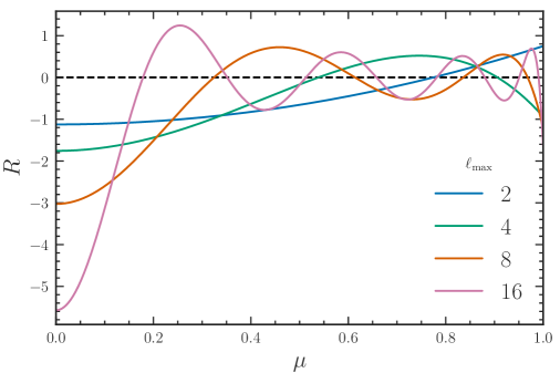
Figure 1: The leakage of a transverse $\mu=0$ systematic into $\mu>0$ power as a function of the maximum multipole used to reconstruct the observed power $P(k,\mu)$. We plot the response of this error, as given in equation 3.5. As multipoles are measured to larger $\ell_{\rm max}$, the contamination is better isolated around the origin, $\mu=0$.

The oscillatory structure of the response in figure 1 suggests that we can employ a non-uniform binning in $\mu$ for our wedge estimator of section 2.2 in order to localize the effect of the systematic to the first bin and cancel out the contamination in each of the other bins. If we desire to have as many wedge bins as number of observed multipoles (measuring even multipoles up to $\ell_{\rm max}$), then there will be $\ell_{\rm max}/2$ non-contaminated bins. The edges of these bins can be computed from the response in equation 3.5 as

$$\int_{\mu_{i}}^{\mu_{i+1}}d\mu\ \frac{\mathcal{L}_{\ell_{\rm max}+1}(\mu)}{\mu}\equiv 0,\quad i=1,2,\ldots,\ell_{\rm max}/2,$$ (3.6)

where $\mu_{i}$ specifies the left edge of the $i^{\rm th}$ bin, and we have assumed a total of $N_{\mu}=\ell_{\rm max}/2+1$ bins. By construction, we have $\mu_{0}=0$ and $\mu_{\ell_{\rm max}/2+1}=1$. In this notation, the only contaminated bin is the first, ranging from $\mu_{0}<\mu<\mu_{1}$. We show the non-uniform binning for $\ell_{\rm max}=4$ and $\ell_{\rm max}=16$ as the shaded regions in the left panel of figure 2. Generically, the $\mu$ wedges first become wider and then significantly narrower ranging from $\mu=0$ to $\mu=1$. We also show the width of the first, contaminated bin, $\mu_{1}-\mu_{0}$, in the right panel. The edge of the first bin closely follows the result in the uniform case, $\mu_{1}-\mu_{0}=(\ell_{\rm max}/2+1)^{-1}$. Larger $\ell_{\rm max}$ values clearly enable better isolation of the systematic signal in a narrow first bin, and in turn, create a larger $\mu$ range absent of any systematics.

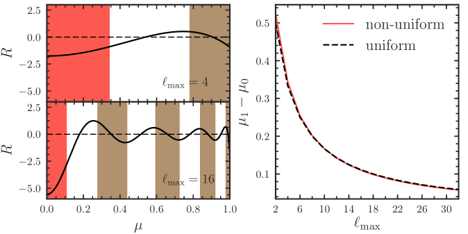
Figure 2: Left: the leakage of a transverse $\mu=0$ systematic into $\mu>0$ power (black) for $\ell_{\rm max}=4$ (top) and $\ell_{\rm max}=16$ (bottom). We show the appropriate non-uniform binning (shaded) that cancels the systematic in all but the first bin (red, shaded). Right: the width of the first $\mu\simeq 0$ bin, given by $\mu_{1}-\mu_{0}$, for the cases of non-uniform (red) and uniform (black, dashed) bins.

3.2 Verification with simulations

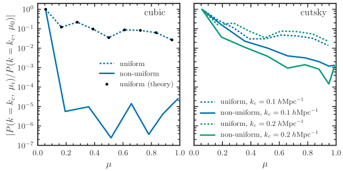
Figure 3: The amplitude of a contaminating spike in 9 $P(k,\mu)$ wedges relative to its amplitude in the first $\mu$ bin for cubic simulation boxes (left) and for cutsky mock catalogs with the BOSS DR12 selection function imposed (right). Wedges are computed from even multipoles up to $\ell_{\rm max}=16$. The mock catalogs contain uniformly clustered objects with a density field modulated via a sinusoidal function in the plane of the sky, causing a large systematic spike in Fourier space at $k=k_{c}$. We show results for both uniform $\mu$ binning (dotted) and the non-uniform (solid) scheme discussed in §3.1.

We verify the utility of the non-uniform binning scheme discussed in §3.1 using simulated density fields. We generate uniformly clustered catalogs of discrete objects and simulate an example systematic signal by modulating the amplitude of the density field in the plane of the sky. We use a sinusoidal function for this modulation, which creates a large contaminating spike in Fourier space at a specific wavenumber, $k=k_{c}$. We perform this test for both periodic boxes and for mock catalogs where the geometry of the DR12 BOSS CMASS sample has been imposed [6, 41]. We denote these latter mocks as cutsky mocks. For the cubic boxes, we simply choose the $z$ axis of the box to be the line-of-sight and modulate the amplitude of the density field in the ($x$,$y$) plane. For the cutsky mocks, which provide the angular and redshift coordinates of objects, we apply the sinusoidal variation as a function of right ascension and declination. We perform these tests for 50 cubic boxes of side length $L_{\rm box}=2600\;h^{-1}\mathrm{Mpc}$ and for 84 cutsky catalogs and compute the average results to reduce noise.

We now compare our simulated results with the theoretical expectations from section 3.1. Because the catalogs are uniformly clustered, the true signal is a constant shot noise that we can subtract from the results. We measure the clustering wedges in both uniform and non-uniform bins and compare the amplitude of the contaminating spike at $k=k_{c}$ for each wedge relative to its amplitude in the first $\mu$ bin. The wedges are computed using even multipoles up to $\ell_{\rm max}=16$, which results in 9 $\mu$ wedges. The left panel of figure 3 shows the results for the cubic boxes. We obtain near-perfect cancellation of the systematic when using non-uniform bins, isolating the contamination to only the first bin at $\mu\simeq 0$. On the other hand, all wedges remain contaminated when using a uniform binning scheme. These results for uniform binning also agree well with our theoretical expectation (shown as black points), given the response in equation 3.5.

The removal of the systematic contamination using the cutsky catalogs, shown in the right panel of figure 3, is not as prominent as in the cubic case. However, the non-uniform binning does reduce the amplitude of the systematic for all wedges, as compared to the uniform scheme, and this reduction is as large as an order of magnitude for most bins. We perform two separate tests for the cutsky mocks, introducing systematic spikes at $k_{c}=0.1\;h\mathrm{Mpc}^{-1}$ and at $k_{c}=0.2\;h\mathrm{Mpc}^{-1}$. We find varying levels of success in eliminating the systematic for these two cases, suggesting some unaccounted for $k$-dependence in the optimal binning scheme. It is likely that the survey geometry, which is not present in the cubic case, complicates the simple model discussed in section 3.1. In the cutsky case, the estimator measures the power spectrum convolved with the window function. In particular, the systematic signal is also convolved with the window function, which mixes $k$ and $\mu$ modes and invalidates our simple modeling assumptions in equation 3.1. We expect the window function to be isotropic and have less influence on small scales (large $k$); this is the trend we find in our results, as we find better cancellation of the systematic in the case of $k_{c}=0.2\;h\mathrm{Mpc}^{-1}$. We explore the effects of the window function on our non-uniform binning scheme in more detail in the next section.

3.3 A toy model for window function effects

Here, we outline a toy model to provide a qualitative understanding of the window function’s impact on systematic removal. We show that the window function couples to the transverse systematic, effectively re-normalizing all of its coefficients in the Legendre basis and thus implying a different choice of non-uniform bin boundaries relative to the window-free case for systematic elimination.

We model the window function as a spherical top-hat in configuration space with radius $R$, so that

$$w(\mathbf{k};R)=\frac{3j_{1}(kR)}{kR},$$ (3.7)

where $j_{1}$ is the spherical Bessel function of order one. The observed systematic is then convolved with the square of the window function as

$$P_{c}^{\rm win}(k,\mu)=\left\{w^{2}(k^{\prime})\star P_{c}(k^{\prime})\delta_{\mathrm{D}}(\mu)\right\}(\mathbf{k}),$$ (3.8)

where star denotes convolution. We note that $P_{c}^{\rm win}(k,\mu)$ remains a function only of $|\mathbf{k}|$ and $\mu$ if the window function is isotropic, as in our toy model. We may evaluate this convolution using the Convolution Theorem, which gives

$$\left\{w^{2}(k^{\prime})\star P_{c}(k^{\prime})\delta_{\mathrm{D}}(\mu)\right\}(k,\mu) =$$

$$\operatorname{FT}\left\{\operatorname{FT}^{-1}\{w^{2}(k^{\prime})\}(r)\;\operatorname{FT}^{-1}\{P_{c}(k^{\prime})\delta_{\mathrm{D}}(\mu)\}(r)\right\}(k,\mu).$$ (3.9)

We first evaluate the inverse Fourier transform (FT) of $w^{2}(k)$. Applying the Convolution Theorem, the desired inverse FT is the convolution of two spherical top-hats, each of radius $R$ with centers separated by $r$. The overlap integral is given by the volume $V_{\rm lens}(r;R)$ of the spherical lens enclosed by both spheres when they are separated by $r$ [42],

$$V_{\rm lens}(r;R)=\frac{\pi}{12}(4R+r)(2R-r)^{2}.$$ (3.10)

This result gives the first term inside the outer curly brackets in equation 3.3. We now seek the second term, the inverse FT of the systematic. Writing the Delta function using its Legendre expansion (equation 3.2) and then expanding the Legendre polynomials into spherical harmonics using the spherical harmonic addition theorem, we find

$$P_{c}(k^{\prime})\delta_{\mathrm{D}}(\mu)=P_{c}(k^{\prime})\sum_{\ell=0}^{\infty}\delta_{\ell}\frac{4\pi}{2\ell+1}\sum_{m=-\ell}^{\ell}Y_{\ell m}(\mathbf{\hat{k}}^{\prime})Y_{\ell m}^{*}(\mathbf{\hat{n}}),$$ (3.11)

where $\delta_{\ell}$ is defined in equation 3.2. The inverse FT can then be obtained by expanding the relevant exponential via the plane wave expansion into spherical Bessel functions and spherical harmonics (e.g., [30], equation 16.52) and invoking orthogonality, leading to

$$\operatorname{FT}^{-1}\left\{P_{c}(k^{\prime})\delta_{\mathrm{D}}(\mu)\right\}(r)=\sum_{\ell=0}^{\infty}S_{\ell}(r)\mathcal{L}_{\ell}(\mu),$$ (3.12)

where $\mu=\mathbf{\hat{r}}\cdot\mathbf{\hat{n}}$ and

$$S_{\ell}(r)=\int\frac{k^{\prime 2}\mathrm{d}k^{\prime}}{2\pi^{2}}j_{\ell}(k^{\prime}r)P_{c}(k^{\prime}).$$ (3.13)

We now have both terms in the outer curly brackets of equation 3.3 and simply require their product’s Fourier transform to obtain $P_{c}^{\rm win}(k,\mu)$, the systematic observed in the presence of the window function.

Expanding the Legendre polynomials of equation 3.12 into spherical harmonics using the addition theorem, again expanding the exponential via the plane wave expansion, and invoking orthogonality, we find

$$P_{c}^{\rm win}(k,\mu)=\sum_{\ell=0}^{\infty}\mathcal{L}_{\ell}(\mu)\delta_{\ell}\int r^{2}\mathrm{d}r\;V_{\rm lens}(r;R)S_{\ell}(r)j_{\ell}(kr).$$ (3.14)

We pause to examine the limit where $R\to\infty$ and hence $V_{\rm lens}(r;R)$ is independent of $r$ and can be taken outside the integral; this corresponds to a boundary-free survey. In this limit, the integral over $r$ can be performed by substituting equation 3.13 and invoking the orthogonality relation for spherical Bessel functions and we recover that $P_{c}^{\rm win}(k,\mu)\to P_{c}(k)\delta_{\mathrm{D}}(\mu)$.

We see that in general, in the presence of an isotropic window function, the coefficients of the Legendre expansion of $P_{c}(k,\mu)$ change and are no longer given by the simple relation $\delta_{\ell}=(2\ell+1)/2\;\mathcal{L}_{\ell}(0)$. Importantly, they now have $k$-dependence, as the window function mixes the purely isotropic systematic amplitude $P_{c}(k)$ with the $\mu$-dependent Delta function. The non-uniform wedge boundaries of the previous section were set by the condition that for a given wedge, the sum of averaged Legendre polynomials weighted by the Delta function’s coefficients would vanish. Here, we see that changing these coefficients simply means this criterion is satisfied for a different non-uniform binning scheme.

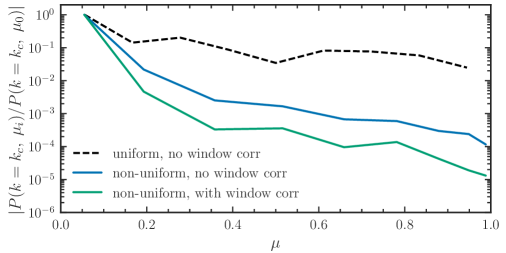
Figure 4: The amplitude of a systematic spike in 9 $P(k,\mu)$ wedges for a uniform clustering field with a toy-model selection function imposed as described in §3.3. When using a non-uniform binning scheme and accounting for window function effects, we can increase the success of the systematic removal by roughly an order of magnitude.

We use simulations to examine the effectiveness of our non-uniform binning scheme in the presence of this toy model window function. We apply a spherical top-hat window function of radius $R=780\;h^{-1}\mathrm{Mpc}$ to a uniformly clustered density field in a cubic box of side length $L_{\mathrm{box}}=2600\;h^{-1}\mathrm{Mpc}$. As in previous sections, we model the systematic with a sinusoidal modulation of the density field in the $(x,y)$ plane, assuming the $z$ axis represents the line-of-sight. This modulation generates a spike in Fourier space at $k=k_{c}$, corresponding to the wavelength of the modulation. We once again use the measured multipoles to estimate wedges in non-uniform bins, and compare the results with and without accounting for the window function corrections in equation 3.14. We present this comparison in figure 4, which shows that by accounting for the window function, an additional order of magnitude reduction in the systematic signal can be achieved in all but the first $\mu$ wedge. As in previous sections, we find that a uniform $\mu$ binning scheme performs worse than our non-uniform scheme, even when ignoring window function effects.

4 Statistical properties

In this section, we explore the covariance properties of the wedge estimator as a function of $\ell_{\rm max}$ and use a Fisher matrix formalism to describe the effect on the derived parameter constraints when using our non-uniform binning approach to mitigate systematics.

4.1 Covariance

Under the assumption of purely Gaussian statistics, the covariance of the power spectrum $P(k,\mu)$ averaged in bins of $k$ and $\mu$ is [26]

$$\operatorname{Cov}\bigl{[}P(k_{i},\mu_{m}),P(k_{j},\mu_{n})\bigr{]}=\delta_{ij}\delta_{mn}\frac{2}{N_{k_{i}}\Delta\mu_{m}}\!\int\!\frac{4\pi k^{2}\mathrm{d}k}{V_{k_{i}}}\frac{\mathrm{d}\mu}{\Delta\mu_{m}}\,\bigl{[}P(k,\mu)+\bar{n}^{-1}\bigr{]}^{2},$$ (4.1)

where the number density of the sample considered is $\bar{n}$, the volume of the shell in $k$-space is $V_{k_{i}}=4\pi[(k_{i}+\Delta k/2)^{3}-(k_{i}-\Delta k/2)^{3}]/3$, and the number of modes in the $i^{\rm th}$ $k$ bin is $N_{k_{i}}=4\pi k_{i}^{2}\Delta kV_{s}/(2\pi)^{3}$, where $V_{s}$ is the volume of the sample considered. Under the assumption of Gaussian statistics, different clustering wedges are not correlated, as reflected by the Kronecker delta factor $\delta_{mn}$ in equation 4.1.

The computationally-efficient estimator presented in this work does not directly measure the quantity $P(k_{i},\mu_{m})$ that enters into equation 4.1. Rather, we reconstruct power spectrum wedges from a finite set of measured multipoles, up to a specified $\ell_{\rm max}$. Thus, the relevant quantity is the covariance of the multipoles averaged in $k$ bins, which is given by

$$\operatorname{Cov}\bigl{[}\widehat{P}_{\ell}(k_{i}),\widehat{P}_{\ell^{\prime}}(k_{j})\bigr{]}=\delta_{ij}(2\ell+1)(2\ell^{\prime}+1)\frac{2}{N_{k_{i}}}\!\int\!\mathrm{d}\mu\frac{2\pi k^{2}\mathrm{d}k}{V_{k_{i}}}\,\mathcal{L}_{\ell}(\mu)\mathcal{L}_{\ell^{\prime}}(\mu)\bigl{[}P(k,\mu)+\bar{n}^{-1}\bigr{]}^{2},$$ (4.2)

where we see multipoles of different $\ell$ are correlated. From this covariance we can compute the covariance of the wedge estimator in equation 2.10 as

$$\operatorname{Cov}\bigl{[}\widehat{P}(k_{i},\mu_{m}),\widehat{P}(k_{j},\mu_{n})\bigr{]}=\sum_{\ell=0}^{\ell_{\rm max}}\sum_{\ell^{\prime}=0}^{\ell_{\rm max}}\bar{\mathcal{L}}_{\ell}(\mu_{m})\bar{\mathcal{L}}_{\ell^{\prime}}(\mu_{n})\operatorname{Cov}\bigl{[}\widehat{P}_{\ell}(k_{i}),\widehat{P}_{\ell^{\prime}}(k_{j})\bigr{]},$$ (4.3)

where the mean Legendre polynomial across a wedge is given by equation 2.11.

The wedge covariance in equation 4.3 is difficult to further simplify analytically, but before comparing to simulations, we can make further progress using the simplifying assumption of linear theory. In this case, we can use the Kaiser model [14]

$$P(k,\mu)=(1+\beta\mu^{2})^{2}b_{1}^{2}P_{\textrm{r}}(k),$$ (4.4)

where $\beta=f/b_{1}$ is the usual redshift-space distortion parameter, $b_{1}$ is the linear bias parameter, $P_{\textrm{r}}(k)$ is the linear theory real-space power spectrum, and $f$ is the logarithmic growth rate [14]. Now, we can separate the scale and angular dependence in equation 4.3. We leave the scale dependence implicit in our notation to focus on the angular subspace in order to improve clarity. With these assumptions, the wedge covariance becomes

$$\widehat{C}_{mn} \equiv\operatorname{Cov}\bigl{[}\widehat{P}(\mu_{m}),\widehat{P}(\mu_{n})\bigr{]}=\frac{2\gamma_{mn}}{N_{k_{i}}}\overline{P_{\textrm{r}}^{2}},$$ (4.5)

where

$$\overline{P_{\textrm{r}}^{2}}\equiv\int\!\frac{4\pi k^{2}\mathrm{d}k}{V_{k_{i}}}\,P_{\textrm{r}}^{2}(k),$$ (4.6)

and

$$\gamma_{mn}\equiv\sum_{\ell=0}^{\ell_{\rm max}}\sum_{\ell^{\prime}0}^{\ell_{\rm max}}(2\ell+1)(2\ell^{\prime}+1)\bar{\mathcal{L}}_{\ell}(\mu_{m})\bar{\mathcal{L}}_{\ell^{\prime}}(\mu_{n})\int\!\frac{\mathrm{d}\mu}{2}\mathcal{L}_{\ell}(\mu)\mathcal{L}_{\ell^{\prime}}(\mu)(1+\beta\mu^{2})^{4}.$$ (4.7)

From these equations, we see that in the simple Kaiser model, the correlation coefficient between between wedges $\mu_{m}$ and $\mu_{n}$, defined as $\rho_{mn}=\widehat{C}_{mn}/(\widehat{C}_{mm}\widehat{C}_{nn})^{1/2}$ is independent of scale with the amplitude proportional to the quantity $\gamma_{mn}$.

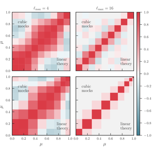
Figure 5: The correlation matrix between $\mu$ wedges measured from cubic box simulations (upper triangle) as compared to linear theory (lower triangle), when using uniform (top row) and non-uniform (bottom row) $\mu$ bins. For 9 $\mu$ wedges, we show results using $\ell_{\rm max}=4$ (left column) and $\ell_{\rm max}=16$ to estimate the wedges from the corresponding multipoles. We find excellent agreement between linear theory and the results measured from simulations.

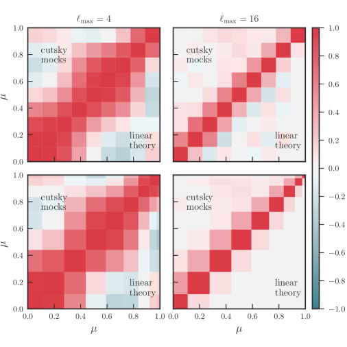
Figure 6: The correlation matrix between $\mu$ wedges measured from realistic cutsky mock catalogs (upper triangle) as compared to linear theory (lower triangle), when using uniform (top row) and non-uniform (bottom row) $\mu$ bins. For 9 $\mu$ wedges, we show results using $\ell_{\rm max}=4$ (left column) and $\ell_{\rm max}=16$ to estimate the wedges from the corresponding multipoles. While there are discrepancies introduced by the window function in comparison to the linear theory expectation, the general trends remain consistent with the periodic box results.

We first compare our simple theoretical modeling to the wedge covariance measured from 990 independent Quick Particle Mesh (QPM) periodic simulations [43] at a redshift of $z=0.55$ and with a box size of $L_{\rm box}=2560\;h^{-1}\mathrm{Mpc}$. These simulations were designed to mimic the clustering of the BOSS CMASS sample, with a linear bias of $b_{1}\sim 2$ at $z\sim 0.5$. We estimate the clustering wedges using the measured multipoles up to a specified $\ell_{\rm max}$ and use the 990 realizations to estimate the covariance of the wedges. We show the resulting correlation matrix between separate $\mu$ wedges in figure 5 and compare to the linear Kaiser result from equation 4.7. We perform this comparison using both non-uniform (bottom row) and uniform (top row) binning schemes, as well as for $\ell_{\rm max}=4$ (left column) and $\ell_{\rm max}=16$ (right column). In all cases, the number of wedges is fixed to $N_{\mu}=9$. We find excellent agreement between a simple Kaiser model with $\beta=0.35$ and the simulation results. As expected, we find the wedges to be significantly more correlated when using only three multipoles to reconstruct nine $\mu$ wedges, as is the case for $\ell_{\rm max}=4$, than when using nine measured multipoles, as for $\ell_{\rm max}=16$. Furthermore, in the case of $\ell_{\rm max}=16$, we find that our non-uniform binning scheme achieves a significantly more diagonal covariance matrix between wedges, as seen in the right column of figure 5. As the matrix becomes more diagonal, the covariance is better approximated by the Gaussian case, where the clustering wedges are fully independent.

We also compare our Kaiser modeling to a set of cutsky mock catalogs that include selection function effects, although we do not expect the simulation results to be well-described by this theoretical model in this case. We use a set of 84 mock catalogs which mimic the radial and angular selection functions of the BOSS DR12 CMASS sample [41, 6]. They model the true geometry, volume, and redshift distribution of the CMASS sample and were constructed from a set of seven independent, periodic box $N$-body simulations with the same cosmology and a side length of $L_{\mathrm{box}}=2600\ h^{-1}\mathrm{Mpc}$. Each of the 84 mock catalogs is an independent realization, and the clustering of these cutsky catalogs is very similar overall to the BOSS CMASS sample at $z\sim 0.5$. As was done for the cubic box simulations, we compare simulation and theory for the correlation matrix for nine $\mu$ wedges using $\ell_{\rm max}=4$ and $\ell_{\rm max}=16$. These results are presented in figure 6. As expected, the cutsky simulation results are not as well-described by the Kaiser model as in the cubic case due to window function effects. However, the general trends in the covariance are similar for the cutsky case as for the cubic case. Importantly, we once again find that using a higher $\ell_{\rm max}$ at fixed $N_{\mu}$ de-correlates the wedges and that the covariance is more diagonal when using our non-uniform binning scheme.

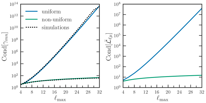
Figure 7: Left: the condition number of the covariance matrix $\gamma_{mn}$, assuming a linear Kaiser model with $\beta=0.35$, as compared to the result computed from the 990 QPM simulations (black). The simulation results have been re-normalized to match the theoretical condition number at $\ell_{\rm max}=4$. Right: the condition number of the matrix specifying the mean Legendre polynomial across each $\mu$ wedge $\bar{L}_{\ell\mu}$ (right), as given by (2.11). We see that the wedge covariance matrix becomes ill-conditioned for large $\ell_{\rm max}$ values when using a uniform binning scheme, driven by the fact that the transformation matrix $\bar{\mathcal{L}}_{\mu\ell}$ also becomes ill-conditioned.

An additional disadvantage of using bins uniform in $\mu$ is that the wedge covariance matrix quickly becomes ill-conditioned for high $\ell_{\rm max}$. This can be seen in figure 7, where the left panel shows the condition number of the $\gamma_{mn}$ matrix as a function of $\ell_{\rm max}$ for both uniform and non-uniform bins. Here, the condition number of a matrix M is defined as the ratio of its smallest to largest singular values, computed using Singular Value Decomposition (SVD) (e.g., [44]). The SVD of a matrix is defined as $\mathbf{M}=\mathbf{U}\mathbf{\Sigma}\mathbf{V}^{T}$, where $\mathbf{\Sigma}$ is a diagonal matrix with the singular values along the diagonal. We find similar trends for the condition number of the covariance matrix for our theoretical results assuming a linear Kaiser model with $\beta=0.35$ and for results computed from the 990 QPM boxes. Both uniform and non-uniform binning result in a reasonable condition number for $\ell_{\rm max}=4$, but the matrix in the uniform case becomes increasingly singular as $\ell_{\rm max}$ increases. In such a case, the inversion of the covariance, which is a necessary step of any likelihood analysis, becomes numerically unstable. This behavior at large $\ell_{\rm max}$ is largely driven by the $\bar{\mathcal{L}}_{\ell\mu}$ matrix, which defines the contribution of a multipole of order $\ell$ to a given $\mu$ wedge. The condition number of this matrix is shown in the right panel of figure 7, and its behavior mirrors that of the full covariance matrix.

The functional form of $\mathcal{L}_{\ell}(\mu)$ can provide some insight into the large condition number of the covariance matrix when using uniformly spaced bins. The Legendre polynomial of order $\ell$ oscillates around zero, and the frequency of the oscillation increases with increasing $\mu$. For large $\ell_{\rm max}$, there exist bins at $\mu\sim 1$ where the Legendre polynomial exhibits a positive/negative symmetry across the bin, and thus, the average value cancels very nearly to zero. This presents problems in equation 2.10, where our measured multipoles are weighted by the mean Legendre polynomial. These issues are mitigated by our non-uniform bins, which were constructed such that the width of the bins decreases as a function of $\mu$, just as the Legendre polynomials oscillate more quickly. Thus, the bin cancellation is mostly avoided when non-uniform bins are used and the condition number of the resulting covariance matrix remains stable, even at large $\ell_{\rm max}$. Such a binning scheme becomes appealing for clustering analyses, even if systematic mitigation is not the primary goal.

4.2 Fisher information

We can evaluate the information content of our wedge estimator as a function of $\ell_{\rm max}$ using the Fisher matrix formalism. As in section 4.1, we assume a simple linear Kaiser model (equation 4.4), where the parameter vector of interest is $\mathbf{p}=(b_{1}\sigma_{8},f\sigma_{8})$. For clarity, we also suppress the $k$ indexing here, as the $\mu$ and $k$ dependence of the covariance is fully separable for the Kaiser model. Assuming a Gaussian likelihood function for the clustering wedge observables, we can express the Fisher matrix as

$$F_{ij}=\sum_{m=0}^{N_{\mu}-1}\sum_{n=0}^{N_{\mu}-1}\frac{\partial P(\mu_{m})}{\partial p_{i}}\widehat{C}_{mn}^{-1}\frac{\partial P(\mu_{n})}{\partial p_{j}},$$ (4.8)

where $N_{\mu}$ is the number of (non-uniform) $\mu$ bins, $P(\mu_{n})$ is the theoretical Kaiser model averaged over the $\mu_{n}$ wedge, and the covariance between the measured wedges $\widehat{C}_{mn}$ is given by equation 4.5. We can also use this formalism to quantify the cost of removing the first $\mu$ bin when using our non-uniform binning scheme. In this case, the Fisher matrix is given by

$$F^{\mu\not\simeq 0}_{ij}=\sum_{m=1}^{N_{\mu}-1}\sum_{n=1}^{N_{\mu}-1}\frac{\partial P(\mu_{m})}{\partial p_{i}}\widehat{C}_{mn}^{-1}\frac{\partial P(\mu_{n})}{\partial p_{j}},$$ (4.9)

where we have explicitly removed the contribution from the $\mu_{0}$ wedge to the double sum in this equation.

We show the Fisher information for the auto-correlations of $b_{1}\sigma_{8}$ and $f\sigma_{8}$, as well as their cross correlation, as a function of $\ell_{\rm max}$ in figure 8. Results are computed for the non-uniform $\mu$ binning scheme presented in section 3.1, assuming a value of $\beta=f/b_{1}=0.35$ for the Kaiser model. The left panel shows the information content when using all $\mu$ bins, and as expected, the information content saturates at $\ell_{\rm max}=4$ because only the $\ell=0,2,$ and $4$ multipoles are non-zero in the Kaiser model. In the right panel of this figure, we show the Fisher information when we exclude the first $\mu$ bin from the analysis. In this case, the information on $b_{1}\sigma_{8}$ is partially lost, approximately proportional to the width of the missing wedge. However, the information on $f\sigma_{8}$ remains relatively unaffected by the missing wedge. The first wedge at $\mu\simeq 0$ is a prominent source of information on the amplitude of the power spectrum, as parametrized by $b_{1}\sigma_{8}$, but contains little information on the $\mu$ dependence of the clustering.

The inverse of the Fisher matrix provides an estimate of the marginalized error on a given parameter, such that the error on the parameter $A$ is given by $\sigma_{A}=(F^{-1})_{AA}^{1/2}$. Thus, we can use the Fisher formalism to evaluate the change in the parameter uncertainties when excluding the first $\mu\simeq 0$ wedge in the presence of a transverse systematic. We show this fractional change for $b_{1}\sigma_{8}$ and $f\sigma_{8}$ as a function of $\ell_{\rm max}$ in figure 9, and we find the loss of constraining power drops rapidly with $\ell_{\rm max}$. For $\ell_{\rm max}=16$, we find $\sim 7$% and $\sim 13$% increases in the uncertainties on $f\sigma_{8}$ and $b_{1}\sigma_{8}$, respectively, as compared to $\sim 54$% and $\sim 92$% for $\ell_{\rm max}=4$. With a reasonably large choice for $\ell_{\rm max}$, we can exclude the contaminated $\mu\simeq 0$ bin with only marginal losses for the parameter constraints of interest.

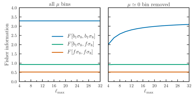
Figure 8: The Fisher information for the parameter vector $\mathbf{p}=(b_{1}\sigma_{8},f\sigma_{8})$ for our wedge estimator using non-uniform $\mu$ bins, in the case of the linear theory Kaiser model. We show results as a function of the maximum multipole used to reconstruct the clustering wedges, as well as the case when using all $\mu$ bins (left) and when excluding the first $\mu$ bin (right). A linear Kaiser model with $\beta=0.35$ has been assumed.

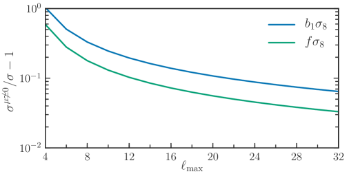
Figure 9: The fractional change in the uncertainties in $b_{1}\sigma_{8}$ and $f\sigma_{8}$ when using non-uniform $\mu$ wedges and excluding the first $\mu\simeq 0$ wedge from the analysis, as determined from the Fisher matrix. A linear Kaiser model with $\beta=0.35$ has been assumed.

5 Conclusions

In this work, we have presented an optimal estimator for the anisotropic power spectrum multipoles that is valid in the local plane-parallel approximation. Our implementation eliminates redundancy present in previous algorithms [22, 23]. These works rely on a Cartesian decomposition of the Legendre basis to write the power spectrum estimator of [17] using Fast Fourier Transforms. We improve upon them by using a spherical harmonic decomposition of the Legendre polynomials, motivated by the approach of [24] for the anisotropic 2PCF. The method presented here is substantially faster than previous anisotropic power spectrum algorithms and renders calculation of multipoles to high $\ell_{\rm max}$ computationally feasible. For a given multipole of order $\ell$, our method requires only $2\ell+1$ FFTs rather than the $(\ell+1)(\ell+2)/2$ FFTs of the Cartesian approach. For the highest $\ell_{\rm max}$ used in this work, $\ell_{\rm max}=16$, our approach is $\sim 3.4\times$ faster than previous works, using 153 FFTs as opposed to 525.

Our estimator’s significant reduction in wall-clock time allows construction of finely-binned wedges in $P(k,\mu)$ by combining multipoles up to high $\ell_{\rm max}$. We show that narrow $\mu$ bins are particularly advantageous for mitigating the effects of systematic contamination in the plane of the sky, as is often the case for galaxy surveys (e.g., [27]). In the presence of such an angular systematic signal, we show that a non-uniform binning scheme in $\mu$ can effectively isolate the contamination to the first $\mu\simeq 0$ wedge and that the systematic contributions to all other bins can be eliminated. We have verified the effectiveness of our non-uniform bins on both periodic simulations and realistic mock catalogs that have a survey selection function. We have demonstrated with a toy model that a survey selection function mixes the $k$ and $\mu$ dependence of the systematic signal, introducing $k$-dependence into the optimal non-uniform wedge boundaries. However, the systematic signal can still be reduced even when ignoring these effects. When analyzing galaxy survey data, knowledge of the window function and realistic simulations can be used to choose the optimal binning to reduce transverse systematics.

We have also explored the statistical properties of the wedge estimator as a function of the maximum measured multipole $\ell_{\rm max}$. We show using linear theory that the covariance of the wedge estimator quickly becomes ill-conditioned for large $\ell_{\rm max}$ when using uniform bins, and we verify this finding with simulations. Consequently, when using uniform bins the covariance inversion is numerically unstable, creating a significant barrier for any likelihood analysis. On the other hand, the non-uniform binning scheme described in this work remains well-conditioned for all $\ell_{\rm max}$ values, enabling its inversion and use in model fitting. We also show that at a fixed number of $\mu$ wedges, using larger values of $\ell_{\rm max}$ de-correlates separate wedges, and that the covariance matrix of wedges using non-uniform bins is more diagonal than in the uniform case. With a Fisher analysis assuming linear theory, we have demonstrated that the uncertainty on $f\sigma_{8}$ inflates by $\sim 7$% with $\ell_{\rm max}=16$ when excluding the first $\mu$ wedge, assuming it is fully contaminated by systematics, as compared to a 54% increase with $\ell_{\rm max}=4$. Even larger choices for $\ell_{\rm max}$ can further reduce this increase and should be explored in more detail for future RSD analyses in the presence of transverse (angular) systematics.

We note that similar techniques as those presented in this paper can be applied to clustering wedges in configuration space. However, the choice of optimal non-uniform bins to remove systematics is further complicated for a correlation function analysis, as the systematic signal is no longer localized to $\mu=0$. Importantly, the optimal binning choice becomes a function of both the separation perpendicular and parallel to the line-of-sight, $r_{\perp}$ and $r_{\parallel}$, which introduces additional modeling complexity. Similar techniques in configuration space should be further explored to assess their effectiveness at minimizing the effects of angular systematics.

Finally, we also point out that, as shown in [19] for the anisotropic 2PCF, slight generalizations of the local plane parallel multipole estimates can be combined to yield the separation midpoint or angle bisector method-based multipoles. This point is important because it enables midpoint and bisector-based multipoles to be obtained by FFTs. As the relevant geometry for anisotropic clustering is the same in Fourier space and configuration space, combining [19] with the results of this work will enable estimation of midpoint or bisector-based multipoles to very high $\ell_{\rm max}$ with FFTs, relevant for properly handling wide-angle effects in next-generation surveys.

The improvements to the power spectrum estimator presented in this work will prove valuable for next generation redshift surveys such as DESI [39, 45, 46] and Euclid [47] both for the data measurement and for the covariance estimation, which requires analyzing a large number of mock catalogs. Given these surveys’ large volumes and consequent high statistical precision, an unprecedented level of systematics control is required. The non-uniform clustering wedges described in this work will be important in this regard for DESI (recently described in [27]). In the future, these methods should be developed and further tested on realistic end-to-end simulations of upcoming surveys.

References

- [1] C. Wagner, V. Müller and M. Steinmetz, Constraining dark energy via baryon acoustic oscillations in the (an)isotropic light-cone power spectrum, A&A 487 (Aug., 2008) 63–74, [0705.0354].
- [2] M. Shoji, D. Jeong and E. Komatsu, Extracting Angular Diameter Distance and Expansion Rate of the Universe From Two-Dimensional Galaxy Power Spectrum at High Redshifts: Baryon Acoustic Oscillation Fitting Versus Full Modeling, ApJ 693 (Mar., 2009) 1404–1416, [0805.4238].
- [3] D. J. Eisenstein, I. Zehavi, D. W. Hogg, R. Scoccimarro, M. R. Blanton, R. C. Nichol et al., Detection of the Baryon Acoustic Peak in the Large-Scale Correlation Function of SDSS Luminous Red Galaxies, ApJ 633 (Nov., 2005) 560–574, [astro-ph/0501171].
- [4] S. Cole, W. J. Percival, J. A. Peacock, P. Norberg, C. M. Baugh, C. S. Frenk et al., The 2dF Galaxy Redshift Survey: power-spectrum analysis of the final data set and cosmological implications, MNRAS 362 (Sept., 2005) 505–534, [arXiv:astro-ph/0501174].
- [5] Z. Slepian, D. J. Eisenstein, J. R. Brownstein, C.-H. Chuang, H. Gil-Marín, S. Ho et al., Detection of Baryon Acoustic Oscillation Features in the Large-Scale 3-Point Correlation Function of SDSS BOSS DR12 CMASS Galaxies, ArXiv e-prints (July, 2016) , [1607.06097].
- [6] S. Alam, M. Ata, S. Bailey, F. Beutler, D. Bizyaev, J. A. Blazek et al., The clustering of galaxies in the completed SDSS-III Baryon Oscillation Spectroscopic Survey: cosmological analysis of the DR12 galaxy sample, ArXiv e-prints (July, 2016) , [1607.03155].
- [7] A. J. Ross, F. Beutler, C.-H. Chuang, M. Pellejero-Ibanez, H.-J. Seo, M. Vargas-Magaña et al., The clustering of galaxies in the completed SDSS-III Baryon Oscillation Spectroscopic Survey: observational systematics and baryon acoustic oscillations in the correlation function, MNRAS 464 (Jan., 2017) 1168–1191, [1607.03145].
- [8] M. Vargas-Magaña, S. Ho, S. Fromenteau and A. J. Cuesta, The clustering of galaxies in the SDSS-III Baryon Oscillation Spectroscopic Survey: Effect of smoothing of density field on reconstruction and anisotropic BAO analysis., MNRAS (Jan., 2017) .
- [9] F. Beutler, H.-J. Seo, A. J. Ross, P. McDonald, S. Saito, A. S. Bolton et al., The clustering of galaxies in the completed SDSS-III Baryon Oscillation Spectroscopic Survey: baryon acoustic oscillations in the Fourier space, MNRAS 464 (Jan., 2017) 3409–3430, [1607.03149].
- [10] H. Gil-Marín, W. J. Percival, A. J. Cuesta, J. R. Brownstein, C.-H. Chuang, S. Ho et al., The clustering of galaxies in the SDSS-III Baryon Oscillation Spectroscopic Survey: BAO measurement from the LOS-dependent power spectrum of DR12 BOSS galaxies, MNRAS 460 (Aug., 2016) 4210–4219, [1509.06373].
- [11] P. Creminelli, A. Nicolis, L. Senatore, M. Tegmark and M. Zaldarriaga, Limits on non-Gaussianities from WMAP data, Journal of Cosmology and Astro-Particle Physics 5 (May, 2006) 4–+, [arXiv:astro-ph/0509029].
- [12] V. Desjacques and U. Seljak, Primordial non-Gaussianity from the large-scale structure, Classical and Quantum Gravity 27 (June, 2010) 124011, [1003.5020].
- [13] C. Alcock and B. Paczynski, An evolution free test for non-zero cosmological constant, Nature 281 (Oct., 1979) 358–+.
- [14] N. Kaiser, Clustering in real space and in redshift space, MNRAS 227 (July, 1987) 1–21.
- [15] L. Guzzo, M. Pierleoni, B. Meneux, E. Branchini, O. Le Fèvre, C. Marinoni et al., A test of the nature of cosmic acceleration using galaxy redshift distortions, Nature 451 (Jan., 2008) 541–544, [arXiv:0802.1944].
- [16] A. J. S. Hamilton, Measuring Omega and the real correlation function from the redshift correlation function, ApJ 385 (Jan., 1992) L5–L8.
- [17] K. Yamamoto, M. Nakamichi, A. Kamino, B. A. Bassett and H. Nishioka, A Measurement of the Quadrupole Power Spectrum in the Clustering of the 2dF QSO Survey, PASJ 58 (Feb., 2006) 93–102, [astro-ph/0505115].
- [18] C. Blake, S. Brough, M. Colless, C. Contreras, W. Couch, S. Croom et al., The WiggleZ Dark Energy Survey: the growth rate of cosmic structure since redshift z=0.9, MNRAS 415 (Aug., 2011) 2876–2891, [1104.2948].
- [19] Z. Slepian and D. J. Eisenstein, A new look at lines of sight: using Fourier methods for the wide-angle anisotropic 2-point correlation function, ArXiv e-prints (Oct., 2015) , [1510.04809].
- [20] L. Samushia, E. Branchini and W. J. Percival, Geometric biases in power-spectrum measurements, MNRAS 452 (Oct., 2015) 3704–3709, [1504.02135].
- [21] J. Yoo and U. Seljak, Wide-angle effects in future galaxy surveys, MNRAS 447 (Feb., 2015) 1789–1805, [1308.1093].
- [22] D. Bianchi, H. Gil-Marín, R. Ruggeri and W. J. Percival, Measuring line-of-sight-dependent Fourier-space clustering using FFTs, MNRAS 453 (Oct., 2015) L11–L15, [1505.05341].
- [23] R. Scoccimarro, Fast estimators for redshift-space clustering, Phys. Rev. D 92 (Oct., 2015) 083532, [1506.02729].
- [24] Z. Slepian and D. J. Eisenstein, Accelerating the two-point and three-point galaxy correlation functions using Fourier transforms, MNRAS 455 (Jan., 2016) L31–L35, [1506.04746].
- [25] E. A. Kazin, A. G. Sánchez and M. R. Blanton, Improving measurements of H(z) and DA (z) by analysing clustering anisotropies, MNRAS 419 (Feb., 2012) 3223–3243, [1105.2037].
- [26] J. N. Grieb, A. G. Sánchez, S. Salazar-Albornoz and C. Dalla Vecchia, Gaussian covariance matrices for anisotropic galaxy clustering measurements, MNRAS 457 (Apr., 2016) 1577–1592, [1509.04293].
- [27] L. Pinol, R. N. Cahn, N. Hand, U. Seljak and M. White, Imprint of desi fiber assignment on the anisotropic power spectrum of emission line galaxies, J. Cosmology Astropart. Phys 2017 (2017) 008, [1611.05007].
- [28] H. A. Feldman, N. Kaiser and J. A. Peacock, Power-spectrum analysis of three-dimensional redshift surveys, ApJ 426 (May, 1994) 23–37, [arXiv:astro-ph/9304022].
- [29] F. Beutler, S. Saito, H.-J. Seo, J. Brinkmann, K. S. Dawson, D. J. Eisenstein et al., The clustering of galaxies in the SDSS-III Baryon Oscillation Spectroscopic Survey: testing gravity with redshift space distortions using the power spectrum multipoles, MNRAS 443 (Sept., 2014) 1065–1089, [1312.4611].
- [30] G. B. Arfken, H. J. Weber and F. E. Harris, Mathematical Methods for Physicists (Seventh Edition). Academic Press, Boston, seventh edition ed., 2013.
- [31] Z. Slepian and D. J. Eisenstein, Computing the three-point correlation function of galaxies in O(N^2) time, MNRAS 454 (Dec., 2015) 4142–4158, [1506.02040].
- [32] Z. Slepian and D. Eisenstein, A practical computational method for the anisotropic three-point correlation function, .
- [33] N. Hand and Y. Feng, nbodykit: a massively parallel large-scale structure toolkit, .
- [34] Y. Feng, “pfft-python: a python binding of pfft.” https://github.com/rainwoodman/pfft-python, 2015-2017.
- [35] M. Pippig, Pfft: An extension of fftw to massively parallel architectures, SIAM Journal on Scientific Computing 35 (2013) C213–C236.
- [36] T. S. D. Team, “sympy: a python library for symbolic mathematics.” http://www.sympy.org, 2016-2017.
- [37] E. Sefusatti, M. Crocce, R. Scoccimarro and H. M. P. Couchman, Accurate estimators of correlation functions in Fourier space, MNRAS 460 (Aug., 2016) 3624–3636, [1512.07295].
- [38] Y. P. Jing, Correcting for the Alias Effect When Measuring the Power Spectrum Using a Fast Fourier Transform, ApJ 620 (Feb., 2005) 559–563, [astro-ph/0409240].
- [39] M. Levi, C. Bebek, T. Beers, R. Blum, R. Cahn, D. Eisenstein et al., The DESI Experiment, a whitepaper for Snowmass 2013, ArXiv e-prints (Aug., 2013) , [1308.0847].
- [40] I. Gradshteyn and I. Ryzhik, Table of Integrals, Series, and Products. Academic Press, Boston, seventh edition ed., 2007.
- [41] B. Reid, S. Ho, N. Padmanabhan, W. J. Percival, J. Tinker, R. Tojeiro et al., SDSS-III Baryon Oscillation Spectroscopic Survey Data Release 12: galaxy target selection and large-scale structure catalogues, MNRAS 455 (Jan., 2016) 1553–1573, [1509.06529].
- [42] E. W. Weisstein, “Sphere-sphere intersection.” http://mathworld.wolfram.com/Sphere-SphereIntersection.html, 2017.
- [43] M. White, J. L. Tinker and C. K. McBride, Mock galaxy catalogues using the quick particle mesh method, MNRAS 437 (Jan., 2014) 2594–2606, [1309.5532].
- [44] W. H. Press, S. A. Teukolsky, W. T. Vetterling and B. P. Flannery, Numerical recipes in C. The art of scientific computing. Cambridge: University Press, —c1992, 2nd ed., 1992.
- [45] DESI Collaboration, A. Aghamousa, J. Aguilar, S. Ahlen, S. Alam, L. E. Allen et al., The desi experiment part i: Science,targeting, and survey design, ArXiv e-prints (oct, 2016) , [1611.00036].
- [46] DESI Collaboration, A. Aghamousa, J. Aguilar, S. Ahlen, S. Alam, L. E. Allen et al., The desi experiment part ii: Instrument design, ArXiv e-prints (oct, 2016) , [1611.00037].
- [47] R. Laureijs, J. Amiaux, S. Arduini, J. . Auguères, J. Brinchmann, R. Cole et al., Euclid Definition Study Report, ArXiv e-prints (Oct., 2011) , [1110.3193].