Variable projection methods for an optimized dynamic mode decomposition

Abstract

The dynamic mode decomposition (DMD) has become a leading tool for data-driven modeling of dynamical systems, providing a regression framework for fitting linear dynamical models to time-series measurement data. We present a simple algorithm for computing an optimized version of the DMD for data which may be collected at unevenly spaced sample times. By making use of the variable projection method for nonlinear least squares problems, the algorithm is capable of solving the underlying nonlinear optimization problem efficiently. We explore the performance of the algorithm with some numerical examples for synthetic and real data from dynamical systems and find that the resulting decomposition displays less bias in the presence of noise than standard DMD algorithms. Because of the flexibility of the algorithm, we also present some interesting new options for DMD-based analysis.

37M02, 65P02, 49M02

1 Introduction

Suppose that ${\mathbf{z}}_{j}\in\mathbb{C}^{n}$ are snapshots of a dynamical system $\dot{{\mathbf{z}}}(t)={\mathbf{f}}({\mathbf{z}}(t))$ at equispaced times $t_{j}=j\Delta t$. Let ${\mathbf{A}}$ be the best fit linear operator which maps each ${\mathbf{z}}_{j}$ to ${\mathbf{z}}_{j+1}$. The dynamic mode decomposition (DMD) is defined as the set of eigenvector, eigenvalue pairs of ${\mathbf{A}}$. The DMD is then a way of decomposing the data into dominant modes, each with an associated frequency of oscillation and rate of growth/decay. This is an alternative decomposition to the proper orthogonal decomposition (POD): whereas the DMD provides dynamical information about the system but the modes are not orthogonal, the POD provides orthogonal modes but no dynamical information. As such, the DMD is an enabling data-driven modeling strategy since it provides a best-fit, linear characterization of a nonlinear dynamical system from data alone.

The DMD has its roots in the fluid dynamics community, where it was applied to the analysis of numerical simulations and experimental data of fluid flows [32, 36]. Over the past decade, its popularity has grown and it has been applied as a diagnostic tool, as a means of model order reduction, and as a component of optimal controller design for a variety of dynamical systems. The DMD also has connections to the Koopman spectral analysis of nonlinear dynamical systems, a line of inquiry which has been pursued in, inter alia, [32, 5, 24, 38]. In particular, the DMD shows promise as a tool for the analysis of general nonlinear systems. We will not stress this aspect here but rather focus on the DMD as an algorithm for approximating data by a linear system.

A well-studied pitfall of the DMD is that the computed eigenvalues are biased by the presence of sensor noise [17, 9]. Intuitively, this is a result of the fact that the standard algorithms treat the data pairwise, i.e. snapshot to snapshot rather than as a whole, and favor one direction (forward in time). In [9], Dawson et al. present several methods for debiasing within the standard DMD framework. These methods have the advantage that they can be computed with essentially the same set of robust and fast tools as the standard DMD.

As an alternative, the optimized DMD of [8] treats all of the snapshots of the data at once. This avoids much of the bias of the original DMD but requires the solution of a (potentially) large nonlinear optimization problem. It is believed that the “nonconvexity of the optimization [required for the optimized DMD] potentially limits its utility” [9] but the results of this paper suggest that the optimized DMD should be the DMD algorithm of choice in many settings. We will present some efficient algorithms for computing the optimized DMD and discuss its properties.

The primary computational tool at the heart of these algorithms is the variable projection method [14]. To apply variable projection, the DMD is rephrased as a problem in exponential data fitting (specifically, inverse differential equations), an area of research which has been extensively developed and has many applications [13, 29]. The variable projection method leverages the special structure of the exponential data fitting problem, so that many of the unknowns may be eliminated from the optimization. An additional benefit of these tools is that the snapshots of data no longer need to be taken at regular intervals, i.e. the sample times do not need to be equispaced. We suggest a pair of algorithms, each a modified version of the original algorithm of [13], for computing the optimized DMD and an initialization scheme based on the standard DMD.

The rest of this paper is organized as follows. In Section 2, we present some of the relevant preliminaries of variable projection and the DMD. In Section 3, we present the definition, algorithms, and an initialization scheme for the optimized DMD. In Section 4, we demonstrate the low inherent bias of the algorithm in the presence of noise on some simple examples and present some applications of the method to both synthetic and real data sets, some with snapshots whose sample times are unevenly spaced. The final section contains some concluding thoughts and ideas for further research.

2 Preliminaries

2.1 Notation

Throughout this paper we use mostly standard notation, with some MATLAB style notation for convenience. Matrices are typically denoted by bold, capital letters and vectors by bold, lower-case. Let ${\mathbf{A}}$ and ${\mathbf{B}}$ be matrices and ${\mathbf{v}}$ a vector of length $m$. Then

• $v_{i}$ denotes the $i$th entry of ${\mathbf{v}}$;

• $A_{i,j}$ denotes the entry in the $i$th row and $j$th column of ${\mathbf{A}}$;

• ${\mathbf{v}}_{i}$ denotes the $i$th vector in a sequence of vectors;

• $\bar{{\mathbf{A}}}$ denotes the entrywise complex conjugate of ${\mathbf{A}}$;

• ${\mathbf{A}}^{\intercal}$ denotes the transpose of ${\mathbf{A}}$, which satisfies $A^{\intercal}_{i,j}=A_{j,i}$;

• ${\mathbf{A}}^{*}$ denotes the complex conjugate transpose of ${\mathbf{A}}$, which satisfies ${\mathbf{A}}^{*}=\bar{{\mathbf{A}}^{\intercal}}$;

• ${\mathbf{A}}^{\dagger}$ denotes the Moore-Penrose pseudoinverse of ${\mathbf{A}}$, which satisfies ${\mathbf{A}}{\mathbf{A}}^{\dagger}{\mathbf{A}}={\mathbf{A}}$, ${\mathbf{A}}^{\dagger}{\mathbf{A}}{\mathbf{A}}^{\dagger}={\mathbf{A}}^{\dagger}$, $({\mathbf{A}}{\mathbf{A}}^{\dagger})^{*}={\mathbf{A}}{\mathbf{A}}^{\dagger}$, and $({\mathbf{A}}^{\dagger}{\mathbf{A}})^{*}={\mathbf{A}}^{\dagger}{\mathbf{A}}$;

• ${\mathbf{A}}(i_{1}:i_{2},j_{1}:j_{2})$ denotes the submatrix corresponding to the $i_{1}$th through $i_{2}$th rows and $j_{1}$th through $j_{2}$th columns of ${\mathbf{A}}$.

• ${\mathbf{A}}(:,j)$ denotes the vector given by the $j$th column of ${\mathbf{A}}$;

• ${\mathbf{A}}(:)$ denotes the vector which results by stacking all of the columns of ${\mathbf{A}}$, taken in order;

• ${\mathbf{A}}=\mbox{diag}({\mathbf{v}})$ denotes the square matrix of size $m\times m$ which satisfies $A_{i,i}=v_{i}$ and $A_{i,j}=0$ for $i\neq j$;

• and ${\mathbf{A}}\otimes{\mathbf{B}}$ denotes the Kronecker of ${\mathbf{A}}$ and ${\mathbf{B}}$, e.g. if ${\mathbf{A}}$ is $2\times 2$ then

  (1) $${\mathbf{A}}\otimes{\mathbf{B}}=\begin{pmatrix}A_{1,1}{\mathbf{B}}&A_{1,2}{\mathbf{B}}\\ A_{2,1}{\mathbf{B}}&A_{2,2}{\mathbf{B}}\end{pmatrix}\;.$$

2.2 Variable projection

In this section, we will review some details of the classical variable projection algorithms [14, 20, 13, 12, 27] which are relevant to the optimized DMD and our implementation of the method. We also include a brief coda concerning modern advances in the variable projection framework.

2.2.1 Nonlinear least squares

The variable projection algorithm was originally conceived for the solution of separable nonlinear least squares problems. The vector version of a separable least squares problem is of the form

(2) $$\mbox{minimize}\|{\mathbf{\boldsymbol{\eta}}}-{\boldsymbol{\Phi}}({\boldsymbol{\alpha}}){\boldsymbol{\beta}}\|_{2}\qquad\mbox{ over }{\boldsymbol{\alpha}}\in\mathbb{C}^{k},{\boldsymbol{\beta}}\in\mathbb{C}^{l}\;,$$

where ${\mathbf{\boldsymbol{\eta}}}\in\mathbb{C}^{m}$, ${\boldsymbol{\Phi}}({\boldsymbol{\alpha}})\in\mathbb{C}^{m\times l}$, and $m>l$. A typical example of such a problem is the approximation of a function $\eta(t)$ by a linear combination of $l$ nonlinear functions $\phi_{j}({\boldsymbol{\alpha}},t)$ with coefficients $\beta_{j}$. In this case, we set $\eta_{i}=\eta(t_{i})$ and $\Phi({\boldsymbol{\alpha}})_{i,j}=\phi_{j}({\boldsymbol{\alpha}},t_{i})$ for $m$ sample times $t_{i}$. Here, and in the remainder of the paper, the dependence of ${\boldsymbol{\Phi}}({\boldsymbol{\alpha}})$ on the times $t_{i}$ is implicit.

The key to the variable projection algorithm is the following observation: for a fixed ${\boldsymbol{\alpha}}$, the ${\boldsymbol{\beta}}$ which minimizes $\|{\boldsymbol{\eta}}-{\boldsymbol{\Phi}}({\boldsymbol{\alpha}}){\boldsymbol{\beta}}\|_{2}$ is given by ${\boldsymbol{\beta}}={\boldsymbol{\Phi}}({\boldsymbol{\alpha}})^{\dagger}{\boldsymbol{\eta}}$. With this observation, we can rewrite the minimization problem Eq. 2 in terms of ${\boldsymbol{\alpha}}$ alone, solve for the minimizer $\hat{{\boldsymbol{\alpha}}}$, and recover the coefficients ${\boldsymbol{\beta}}$ corresponding to this minimizer via $\hat{{\boldsymbol{\beta}}}={\boldsymbol{\Phi}}(\hat{{\boldsymbol{\alpha}}})^{\dagger}{\boldsymbol{\eta}}$. It is clear that the minimization problem in ${\boldsymbol{\alpha}}$ alone is equivalent to

(3) $$\mbox{minimize}\dfrac{1}{2}\|{\boldsymbol{\eta}}-{\boldsymbol{\Phi}}({\boldsymbol{\alpha}}){\boldsymbol{\Phi}}({\boldsymbol{\alpha}})^{\dagger}{\boldsymbol{\eta}}\|_{2}^{2}\qquad\mbox{ over }{\boldsymbol{\alpha}}\in\mathbb{C}^{k}\;,$$

where we have squared the error and rescaled for notational convenience.

Typically [20, 13, 12, 27], the Levenberg-Marquardt algorithm [22, 23] is used for the solution of the new minimization problem Eq. 3. This is an iterative procedure for solving Eq. 3, which produces a sequence of vectors ${\boldsymbol{\alpha}}_{i}$ which should converge to a nearby (local) minimizer. Let

(4) $${\boldsymbol{\rho}}({\boldsymbol{\alpha}})={\boldsymbol{\eta}}-{\boldsymbol{\Phi}}({\boldsymbol{\alpha}}){\boldsymbol{\Phi}}({\boldsymbol{\alpha}})^{\dagger}{\boldsymbol{\eta}}$$

denote the residual. We will use ${\boldsymbol{\delta}}_{i}$ to denote the update to ${\boldsymbol{\alpha}}_{i}$, so that ${\boldsymbol{\alpha}}_{i+1}={\boldsymbol{\alpha}}_{i}-{\boldsymbol{\delta}}_{i}$ and assume that a parameter $\nu_{i}$ is specified at each iteration. The Levenberg-Marquardt update is defined to be the solution of

(5) $$\mbox{minimize}\left\|\begin{pmatrix}{\mathbf{J}}({\boldsymbol{\alpha}}_{i})\\ \nu_{i}{\mathbf{M}}({\boldsymbol{\alpha}}_{i})\end{pmatrix}{\boldsymbol{\delta}}_{i}-\begin{pmatrix}{\boldsymbol{\rho}}({\boldsymbol{\alpha}}_{i})\\ 0\end{pmatrix}\right\|_{2}^{2}\qquad\mbox{ over }{\boldsymbol{\delta}}_{i}\in\mathbb{C}^{k}\;,$$

where ${\mathbf{J}}({\boldsymbol{\alpha}}_{i})$ is the Jacobian of ${\boldsymbol{\rho}}({\boldsymbol{\alpha}})$ evaluated at ${\boldsymbol{\alpha}}_{i}$ and ${\mathbf{M}}({\boldsymbol{\alpha}}_{i})$ is a diagonal matrix of scalings such that $M({\boldsymbol{\alpha}}_{i})_{jj}=\|{\mathbf{J}}({\boldsymbol{\alpha}}_{i})(:,j)\|_{2}$. Typically the parameter $\nu_{i}$ is chosen as part of a trust-region method, i.e. $\nu_{i}$ is increased until a step is found so that the new ${\boldsymbol{\alpha}}_{i+1}$ results in a smaller residual. When possible, the parameter $\nu_{i}$ is reduced so that the update is more like a standard Gauss-Newton update, which results in a fast convergence rate. Ruhe and Wedin [35] showed that when superlinear convergence occurs for Gauss-Newton applied to the original problem Eq. 2, then it also occurs for the projected problem Eq. 3. See [23, 28] for more detail on choosing $\nu_{i}$ and the overall structure of the Levenberg-Marquardt method.

In order to apply this method, we must have an expression for the Jacobian of ${\boldsymbol{\rho}}({\boldsymbol{\alpha}})$. Typically, the derivatives of ${\boldsymbol{\Phi}}$ with respect to ${\boldsymbol{\alpha}}$ are known analytically, e.g. they are simple to obtain in the case that $\phi_{j}({\boldsymbol{\alpha}},t)=\exp(\alpha_{j}t)$. We therefore assume that these derivatives are available. In the following, we will leave out the dependence of the matrices on ${\boldsymbol{\alpha}}$ in order to simplify the notation. Let ${\mathbb{P}}_{\Phi}$ denote the orthogonal projection onto the columns of ${\boldsymbol{\Phi}}$, i.e. ${\mathbb{P}}_{\Phi}={\boldsymbol{\Phi}}{\boldsymbol{\Phi}}^{\dagger}$, and ${\mathbb{P}}_{\Phi}^{\perp}$ denote the projection onto the complement of the column space of ${\boldsymbol{\Phi}}$, i.e. ${\mathbb{P}}_{\Phi}^{\perp}={\mathbf{I}}-{\boldsymbol{\Phi}}{\boldsymbol{\Phi}}^{\dagger}$. Note that ${\boldsymbol{\rho}}={\mathbb{P}}_{\Phi}^{\perp}{\boldsymbol{\eta}}$. From Lemma 4.1 of [14], we have

(6) $${\mathbf{J}}(:,j)=\frac{\partial{\boldsymbol{\rho}}}{\partial\alpha_{j}}=-\left({\mathbb{P}}_{\Phi}^{\perp}\dfrac{\partial{\boldsymbol{\Phi}}}{\partial\alpha_{j}}{\boldsymbol{\Phi}}^{\dagger}+\left({\mathbb{P}}_{\Phi}^{\perp}\dfrac{\partial{\boldsymbol{\Phi}}}{\partial\alpha_{j}}{\boldsymbol{\Phi}}^{\dagger}\right)^{*}\right){\boldsymbol{\eta}}\;.$$

Kaufman [20] recommends the approximation

(7) $${\mathbf{J}}(:,j)=\frac{\partial{\boldsymbol{\rho}}}{\partial\alpha_{j}}\approx-{\mathbb{P}}_{\Phi}^{\perp}\dfrac{\partial{\boldsymbol{\Phi}}}{\partial\alpha_{j}}{\boldsymbol{\Phi}}^{\dagger}{\boldsymbol{\eta}}\;,$$

which is accurate for small residuals. This approximation is used in [13] and there is some debate over whether this approximation to the Jacobian is superior to the full expression, see, inter alia, [26, 27]. In our MATLAB implementation [4], we have used the full expression.

All of the terms in the above expression can be computed by making use of the singular value decomposition (SVD) of ${\boldsymbol{\Phi}}$. Let $q$ be the rank of ${\boldsymbol{\Phi}}$. The (reduced) SVD of a matrix ${\boldsymbol{\Phi}}$ provides three matrices ${\mathbf{U}}$, ${\boldsymbol{\Sigma}}$, and ${\mathbf{V}}$ such that ${\boldsymbol{\Phi}}={\mathbf{U}}{\boldsymbol{\Sigma}}{\mathbf{V}}^{*}$, ${\mathbf{U}}\in\mathbb{C}^{m\times q}$ and ${\mathbf{V}}\in\mathbb{C}^{l\times q}$ have orthonormal columns, and ${\boldsymbol{\Sigma}}\in\mathbb{R}^{q\times q}$ is diagonal with nonnegative entries. Given the SVD of ${\boldsymbol{\Phi}}$, we have that

(8) $${\mathbb{P}}_{\Phi}^{\perp}\dfrac{\partial{\boldsymbol{\Phi}}}{\partial\alpha_{j}}{\boldsymbol{\Phi}}^{\dagger}{\boldsymbol{\eta}}=({\mathbf{I}}-{\mathbf{U}}{\mathbf{U}}^{*})\dfrac{\partial{\boldsymbol{\Phi}}}{\partial\alpha_{j}}{\boldsymbol{\beta}}\;,$$

where we have solved for ${\boldsymbol{\beta}}$ using ${\boldsymbol{\beta}}={\mathbf{V}}{\boldsymbol{\Sigma}}^{-1}{\mathbf{U}}^{*}{\boldsymbol{\eta}}$, and

(9) $$\left({\mathbb{P}}_{\Phi}^{\perp}\dfrac{\partial{\boldsymbol{\Phi}}}{\partial\alpha_{j}}{\boldsymbol{\Phi}}^{\dagger}\right)^{*}{\boldsymbol{\eta}}={\mathbf{U}}{\boldsymbol{\Sigma}}^{-1}{\mathbf{V}}^{*}\dfrac{\partial{\boldsymbol{\Phi}}}{\partial\alpha_{j}}^{*}{\boldsymbol{\rho}}\;,$$

where we have used the fact that $({\mathbb{P}}_{\Phi}^{\perp})^{*}{\boldsymbol{\eta}}={\mathbb{P}}_{\Phi}^{\perp}{\boldsymbol{\eta}}={\boldsymbol{\rho}}$.

2.2.2 Variable projection for multiple right hand sides

One of the primary innovations of [13] was the extension of the variable projection method developed above to the case of multiple right hand sides, i.e. to the problem

(10) $$\mbox{minimize}\|{\mathbf{H}}-{\boldsymbol{\Phi}}({\boldsymbol{\alpha}}){\mathbf{B}}\|_{F}\qquad\mbox{ over }{\boldsymbol{\alpha}}\in\mathbb{C}^{k},{\mathbf{B}}\in\mathbb{C}^{l\times n}\;,$$

where ${\mathbf{H}}\in\mathbb{C}^{m\times n}$, ${\boldsymbol{\Phi}}({\boldsymbol{\alpha}})\in\mathbb{C}^{m\times l}$, and $m>l$. A typical example of such a problem is the approximation of $n$ functions $\eta_{p}(t)$, each by a linear combination of $l$ nonlinear functions $\phi_{j}({\boldsymbol{\alpha}},t)$ with coefficients $B_{j,p}$. In this case, we have $H_{i,p}=\eta_{p}(t_{i})$ and $\Phi({\boldsymbol{\alpha}})_{i,j}$ is as before, ${\Phi}({\boldsymbol{\alpha}})_{i,j}=\phi_{j}({\boldsymbol{\alpha}},t_{i})$. We note that the vector of parameters ${\boldsymbol{\alpha}}$ is the same for each function $\eta_{p}$, so that the problem is coupled.

This problem can be solved efficiently using ideas similar to those outlined for the case of a single right hand side above. In order to use the same language as for the vector case, we need to reshape problem Eq. 10. Let ${\boldsymbol{\eta}}={\mathbf{H}}(:)$ and ${\boldsymbol{\beta}}={\mathbf{B}}(:)$. Then Eq. 10 is equivalent to

(11) $$\mbox{minimize}\|{\boldsymbol{\eta}}-{\mathbf{I}}_{n}\otimes{\boldsymbol{\Phi}}({\boldsymbol{\alpha}}){\boldsymbol{\beta}}\|_{2}\qquad\mbox{ over }{\boldsymbol{\alpha}}\in\mathbb{C}^{k},{\boldsymbol{\beta}}\in\mathbb{C}^{ln}\;.$$

For a given ${\boldsymbol{\alpha}}$, the matrix ${\mathbf{B}}$ is given by ${\boldsymbol{\Phi}}^{\dagger}{\mathbf{H}}$ so that the computation of ${\boldsymbol{\beta}}$ can be done in blocked form. Likewise, the computation of ${\boldsymbol{\rho}}$ can be blocked. Let ${\mathbf{P}}={\mathbf{H}}-{\boldsymbol{\Phi}}{\mathbf{B}}$. Then ${\boldsymbol{\rho}}={\mathbf{P}}(:)$. Importantly, the formation of the Jacobian can also be blocked. If we set

(12) $${\mathbf{J}}^{\operatorname{mat}}_{j}=-\left({\mathbb{P}}_{\Phi}^{\perp}\dfrac{\partial{\boldsymbol{\Phi}}}{\partial\alpha_{j}}{\boldsymbol{\Phi}}^{\dagger}+\left({\mathbb{P}}_{\Phi}^{\perp}\dfrac{\partial{\boldsymbol{\Phi}}}{\partial\alpha_{j}}{\boldsymbol{\Phi}}^{\dagger}\right)^{*}\right){\mathbf{H}}\;,$$

then ${\mathbf{J}}(:,j)={\mathbf{J}}^{\operatorname{mat}}_{j}(:)$. As above, if the SVD of ${\boldsymbol{\Phi}}$ is computed, we may write

(13) $${\mathbb{P}}_{\Phi}^{\perp}\dfrac{\partial{\boldsymbol{\Phi}}}{\partial\alpha_{j}}{\boldsymbol{\Phi}}^{\dagger}{\mathbf{H}}=({\mathbf{I}}-{\mathbf{U}}{\mathbf{U}}^{*})\dfrac{\partial{\boldsymbol{\Phi}}}{\partial\alpha_{j}}{\mathbf{B}}\;,$$

where we have solved for ${\mathbf{B}}$ using ${\mathbf{B}}={\mathbf{V}}{\boldsymbol{\Sigma}}^{-1}{\mathbf{U}}^{*}{\mathbf{H}}$, and

(14) $$\left({\mathbb{P}}_{\Phi}^{\perp}\dfrac{\partial{\boldsymbol{\Phi}}}{\partial\alpha_{j}}{\boldsymbol{\Phi}}^{\dagger}\right)^{*}{\mathbf{H}}={\mathbf{U}}{\boldsymbol{\Sigma}}^{-1}{\mathbf{V}}^{*}\dfrac{\partial{\boldsymbol{\Phi}}}{\partial\alpha_{j}}^{*}{\mathbf{P}}\;,$$

where we have used the fact that $({\mathbb{P}}_{\Phi}^{\perp})^{*}{\mathbf{H}}={\mathbb{P}}_{\Phi}^{\perp}{\mathbf{H}}={\mathbf{P}}$.

Because this is the version of the variable projection algorithm used for the computations in this paper, we will briefly discuss its computational cost. The matrices of partial derivatives of ${\boldsymbol{\Phi}}$, i.e.

$${\mathbf{D}}_{j}=\dfrac{\partial{\boldsymbol{\Phi}}}{\partial\alpha_{j}}\;,$$

are often sparse in applications. As this is the case in our application, we will make the simplifying assumption that these matrices have one nonzero column. In our implementation, these matrices are stored in MATLAB sparse matrix format, though there are possibly more efficient ways to leverage the sparsity, see [27] for an example. In what follows, we assume that MATLAB handling of sparse matrix-matrix multiplication is optimal in the sense of operation count. Another simplifying assumption we make is that $l=k$ and that ${\boldsymbol{\Phi}}$ is full rank, i.e. $q=k$.

Each iteration of the algorithm is dominated by the cost of forming the Jacobian, ${\mathbf{J}}$, and solving for the update, ${\boldsymbol{\delta}}$. We have that ${\mathbf{J}}\in\mathbb{C}^{mn\times k}$ and ${\mathbf{M}}\in\mathbb{C}^{k\times k}$ so that the solve for ${\boldsymbol{\delta}}$ is $\mathcal{O}(k^{2}mn)$ using standard linear least squares methods, e.g. a QR factorization. We will consider the cost of computing ${\mathbf{J}}$ in four steps:

1. the cost of the SVD of ${\boldsymbol{\Phi}}$,

2. forming ${\mathbf{B}}$ and ${\mathbf{P}}$,

3. applying formula Eq. 13,

4. and applying formula Eq. 14.
   

For step 1, the SVD of ${\boldsymbol{\Phi}}$ costs $\mathcal{O}(k^{2}m)$ to compute with standard methods. In step 2, ${\mathbf{B}}$ and ${\mathbf{P}}$ are formed via matrix-matrix multiplications which are $\mathcal{O}(kmn)$. Note that steps 1 and 2 are computed once.

In step 3, the order of operations is more important. We rewrite Eq. 13 as

(15) $${\mathbb{P}}_{\Phi}^{\perp}\dfrac{\partial{\boldsymbol{\Phi}}}{\partial\alpha_{j}}{\boldsymbol{\Phi}}^{\dagger}{\mathbf{H}}=\left({\mathbf{D}}_{j}-{\mathbf{U}}\left({\mathbf{U}}*{\mathbf{D}}_{j}\right)\right){\mathbf{B}}\;,$$

where the parentheses determine the order of the matrix multiplications. Forming ${\mathbf{U}}^{*}{\mathbf{D}}_{j}$ costs $\mathcal{O}(km)$ and is itself sparse with one nonzero column. The cost of forming ${\mathbf{U}}({\mathbf{U}}^{*}{\mathbf{D}}_{j})$ is then again $\mathcal{O}(km)$ and is sparse with one nonzero column. Finally, ${\mathbf{D}}_{j}-{\mathbf{U}}({\mathbf{U}}^{*}{\mathbf{D}}_{j})$ is still sparse with one nonzero column so that the last multiplication giving $({\mathbf{D}}_{j}-{\mathbf{U}}({\mathbf{U}}^{*}{\mathbf{D}}_{j})){\mathbf{B}}$ costs $\mathcal{O}(mn)$. Repeating these calculations for each column is then $\mathcal{O}(k^{2}m+kmn)$ in total.

In step 4, the order of operations are again important. We rewrite Eq. 14 as

(16) $$\left({\mathbb{P}}_{\Phi}^{\perp}\dfrac{\partial{\boldsymbol{\Phi}}}{\partial\alpha_{j}}{\boldsymbol{\Phi}}^{\dagger}\right)^{*}{\mathbf{H}}={\mathbf{U}}({\boldsymbol{\Sigma}}^{-1}({\mathbf{V}}^{*}({\mathbf{D}}_{j}^{*}{\mathbf{P}})))\;.$$

Because ${\mathbf{D}}_{j}^{*}$ has one nonzero row, forming ${\mathbf{D}}_{j}^{*}{\mathbf{P}}$ is $\mathcal{O}(mn)$ and the result has one nonzero row. Similarly, it then costs $\mathcal{O}(kn)$ to form ${\mathbf{V}}^{*}({\mathbf{D}}_{j}^{*}{\mathbf{P}})$ but the result is a full matrix of size $k\times n$. The product ${\boldsymbol{\Sigma}}^{-1}({\mathbf{V}}^{*}({\mathbf{D}}_{j}^{*}{\mathbf{P}}))$ simply scales the rows, which costs $\mathcal{O}(kn)$. Finally, forming ${\mathbf{U}}({\boldsymbol{\Sigma}}^{-1}({\mathbf{V}}^{*}({\mathbf{D}}_{j}^{*}{\mathbf{P}})))$ is a dense matrix-matrix multiplication which costs $\mathcal{O}(kmn)$. Repeating these calculations for each column is then $\mathcal{O}(k^{2}n+k^{2}mn)$ in total. This unfavorable scaling, when compared with that of step 3, is part of the appeal of using the approximation Eq. 7.

In the discussion of the optimized DMD, we will take for granted the existence of an algorithm for solving Eq. 10. See, for instance, the original Fortran implementation (follow the URL in [13]). We have also prepared a MATLAB implementation for the computations in this manuscript [4].

2.2.3 Inverse differential equations

In [13], it is observed that the inverse differential equations problem can be phrased as a nonlinear least squares problem with multiple right hand sides. Suppose that ${\mathbf{z}}(t)\in\mathbb{C}^{n}$ is the solution of

(17) $$\dot{{\mathbf{z}}}(t)={\mathbf{A}}{\mathbf{z}}(t)\;,$$

with the initial condition ${\mathbf{z}}(0)={\mathbf{z}}_{0}$. The solution of this problem is known analytically,

(18) $${\mathbf{z}}(t)=e^{{\mathbf{A}}t}{\mathbf{z}}_{0}\;,$$

where we have used the matrix exponential. The inverse linear differential equations problem is to find ${\mathbf{A}}$ given ${\mathbf{z}}(t_{i})$ for $m\geq n$ sample times $t_{i}$. Note that this problem is the natural extension of the DMD to data with arbitrary sample times.

If we assume that ${\mathbf{A}}$ is diagonalizable, we can write

(19) $${\mathbf{z}}(t)=e^{{\mathbf{A}}t}{\mathbf{z}}_{0}=e^{{\mathbf{S}}{\boldsymbol{\Lambda}}t{\mathbf{S}}^{-1}}{\mathbf{z}}_{0}={\mathbf{S}}e^{{\boldsymbol{\Lambda}}t}{\mathbf{S}}^{-1}{\mathbf{z}}_{0}\;,$$

where ${\mathbf{A}}={\mathbf{S}}{\boldsymbol{\Lambda}}{\mathbf{S}}^{-1}$ and ${\boldsymbol{\Lambda}}$ is diagonal. Let the diagonal values of ${\boldsymbol{\Lambda}}$ be given by ${\alpha}_{1},\ldots,{\alpha}_{k}$ and define nonlinear basis functions by $\phi_{j}({\boldsymbol{\alpha}},t)=\exp({\alpha_{j}t})$. If we let ${\boldsymbol{\Phi}}({\boldsymbol{\alpha}})$ and ${\mathbf{H}}$ be defined as above, with $\eta_{p}(t_{i})={z}_{p}(t_{i})$, then

(20) $${\mathbf{H}}={\boldsymbol{\Phi}}({\boldsymbol{\alpha}}){\mathbf{B}}\;,$$

where

(21) $${B}_{i,j}={S}_{j,i}({\mathbf{S}}^{-1}{\mathbf{z}}_{0})_{i}\;$$

are the entries of ${\mathbf{B}}$. Therefore, the inverse differential equations problem can be solved by first solving

(22) $$\mbox{minimize}\|{\mathbf{H}}-{\boldsymbol{\Phi}}({\boldsymbol{\alpha}}){\mathbf{B}}\|_{F}\qquad\mbox{ over }{\boldsymbol{\alpha}}\in\mathbb{C}^{n},{\mathbf{B}}\in\mathbb{C}^{n\times n}\;.$$

Note that $k=l=n$ in this application. The matrix ${\mathbf{A}}$ can then be recovered by observing that the $i$th column of ${\mathbf{B}}^{\intercal}$ is an eigenvector of ${\mathbf{A}}$ corresponding to the eigenvalue ${\alpha}_{i}$.

Remark 2.1.

We note that the variable projection framework also applies immediately to the case that $n>l$, i.e. to the case of fitting an $l$ dimensional linear system to data in a higher dimensional space. The first algorithm presented in Section 3 is the direct result of this observation.

Remark 2.2.

When ${\boldsymbol{\alpha}}$ contains confluent (or nearly confluent) eigenvalues, the matrix ${\boldsymbol{\Phi}}({\boldsymbol{\alpha}})$ will not be full rank (or nearly not full rank). For the case that ${\mathbf{A}}$ truly has confluent (or nearly confluent) eigenvalues, the algorithm will suffer near the solution. In particular, it is difficult to try to approximate dynamics arising from a system with a non-diagonalizable matrix ${\mathbf{A}}$ using exponentials alone. For the purposes of generalizing this method to a larger class of ODE systems, the decomposition proposed as part of “Method 18” in [25] for computing the matrix exponential of a matrix ${\mathbf{C}}$ offers an interesting alternative. In Method 18, ${\mathbf{C}}$ is decomposed as ${\mathbf{C}}={\mathbf{S}}{\mathbf{B}}{\mathbf{S}}^{-1}$, where the matrix ${\mathbf{B}}$ is block-diagonal, with each block upper-triangular. Intuitively, the blocks are selected so that nearly-confluent eigenvalues are grouped together and the condition number of ${\mathbf{S}}$ is kept manageable. If we allow ${\boldsymbol{\Lambda}}$ to be block-diagonal with upper-triangular blocks, then the algorithm for inverse linear systems above could accommodate all matrices. In this case, we may have that $k>l$ and the software will be significantly more complicated. This is the subject of ongoing research and progress will be reported at a later date.

2.2.4 Modern variable projection

The idea at the core of variable projection, reducing the number of unknowns in a minimization problem by exploiting special structure, is not limited in application to unconstrained nonlinear least squares problems. We will not attempt a review of this broad subject here but will point to the applications of [27, 7, 2, 37] for a sense of the types of problems which can be approached. Among the applications are exponential data fitting with constraints, blind deconvolution, and multiple kernel learning. Because of this flexibility, we believe that rephrasing the DMD as a problem in the variable projection framework will provide opportunities for extensions of the DMD, including constrained and robust versions.

In the recent paper [1], Aravkin et al. develop a variable projection method for an interesting variation on the exponential fitting problem. Let ${\boldsymbol{\Phi}}({\boldsymbol{\alpha}})\in\mathbb{C}^{m\times k}$ be made up of columns of exponentials, i.e. $\phi_{j}({\boldsymbol{\alpha}},t)=\exp({\alpha_{j}t})$, as in the previous section and consider a single stream of data ${\boldsymbol{\eta}}\in\mathbb{C}^{m}$. The appropriate number, $k$, of different exponentials to use to approximate the data may be difficult to ascertain a priori. Instead of choosing the correct number ahead of time, one can choose a large $k$ and augment the standard nonlinear least squares problem with a sparsity prior, resulting in the problem

(23) $$\mbox{minimize }f({\boldsymbol{\alpha}},{\boldsymbol{\beta}})=\|{\boldsymbol{\eta}}-{\boldsymbol{\Phi}}({\boldsymbol{\alpha}}){\boldsymbol{\beta}}\|_{2}^{2}+\|{\boldsymbol{\beta}}\|_{1}\mbox{ over }{\boldsymbol{\alpha}}\in\mathbb{C}^{k},{\boldsymbol{\beta}}\in\mathbb{C}^{k}\;.$$

For a fixed ${\boldsymbol{\alpha}}$, the problem in ${\boldsymbol{\beta}}$ alone can be solved using any suitable least absolute shrinkage and selection operator (LASSO) algorithm. In [1], the function

(24) $$\tilde{f}({\boldsymbol{\alpha}})=\min_{\boldsymbol{\beta}}f({\boldsymbol{\alpha}},{\boldsymbol{\beta}})$$

is shown to be differentiable under suitable conditions and a formula for the gradient is derived. This can then be used to solve for the minimizer of $\tilde{f}$ with a nonlinear optimization routine.

The DMD and optimized DMD face similar issues when it comes to determining the appropriate rank $r$. Extending the above idea to the DMD setting is work in progress and will be reported at a later date.

2.3 The DMD

In this section, we will provide some details of the DMD algorithm and discuss its computation and properties, using the notation and definitions of [38].

2.3.1 Exact DMD

The exact DMD is defined for pairs of data $\{({\mathbf{x}}_{1},{\mathbf{y}}_{1}),\ldots,({\mathbf{x}}_{m},{\mathbf{y}}_{m})\}$ which we assume satisfy ${\mathbf{y}}_{j}={\mathbf{A}}{\mathbf{x}}_{j}$, for some matrix ${\mathbf{A}}$. Typically, the pairs are assumed to be given by equispaced snapshots of some dynamical system ${\mathbf{z}}(t)$, i.e. ${\mathbf{x}}_{j}={\mathbf{z}}((j-1)\Delta t)$ and ${\mathbf{y}}_{j}={\mathbf{z}}(j\Delta t)$, but they are not required to be of this form. For most data sets, the matrix ${\mathbf{A}}$ is not determined fully by the snapshots. Therefore, we define the matrix ${\mathbf{A}}$ from the data in a least- squares sense. In particular, we set

(25) $${\mathbf{A}}={\mathbf{Y}}{\mathbf{X}}^{\dagger}\;,$$

where ${\mathbf{X}}^{\dagger}$ is the pseudo-inverse of ${\mathbf{X}}$. The matrix ${\mathbf{A}}$ above is the minimizer of $\|{\mathbf{A}}{\mathbf{X}}-{\mathbf{Y}}\|_{F}$ in the case that ${\mathbf{A}}{\mathbf{X}}={\mathbf{Y}}$ is over-determined and the minimum norm ($\|{\mathbf{A}}\|_{F}$) solution of ${\mathbf{A}}{\mathbf{X}}={\mathbf{Y}}$ in the case that the equation is under-determined [38] ($\|\cdot\|_{F}$ denotes the standard Frobenius norm). We may say that ${\mathbf{A}}$ is the best fit linear system mapping ${\mathbf{X}}$ to ${\mathbf{Y}}$ or, in the typical application, the best fit linear map which advances ${\mathbf{z}}(t)$ to ${\mathbf{z}}(t+\Delta t)$ (this map is sometimes referred to as a forward propagator).

The dynamic mode decomposition is then defined to be the set of eigenvectors and eigenvalues of ${\mathbf{A}}$. Algorithm 1 provides a robust method for computing these values [38].

Algorithm 1 Exact DMD [38]

1. Define matrices ${\mathbf{X}}$ and ${\mathbf{Y}}$ from the data:

   (26) $${\mathbf{X}}=\left({\mathbf{x}}_{1},\ldots,{\mathbf{x}}_{m}\right)\;,\qquad{\mathbf{Y}}=\left({\mathbf{y}}_{1},\ldots,{\mathbf{y}}_{m}\right)\;.$$

2. Take the (reduced) SVD of the matrix ${\mathbf{X}}$, i.e. compute ${\mathbf{U}}$, ${\boldsymbol{\Sigma}}$, and ${\mathbf{V}}$ such that

   (27) $${\mathbf{X}}={\mathbf{U}}{\boldsymbol{\Sigma}}{\mathbf{V}}^{*}\;,$$

   where ${\mathbf{U}}\in\mathbb{C}^{n\times r}$, ${\boldsymbol{\Sigma}}\in\mathbb{C}^{r\times r}$, and ${\mathbf{V}}\in\mathbb{C}^{m\times r}$, with $r$ the rank of ${\mathbf{X}}$.

3. Let $\tilde{{\mathbf{A}}}$ be defined by

   (28) $$\tilde{{\mathbf{A}}}={\mathbf{U}}^{*}{\mathbf{Y}}{\mathbf{V}}{\boldsymbol{\Sigma}}^{-1}\;.$$

4. Compute the eigendecomposition of $\tilde{{\mathbf{A}}}$, giving a set of $r$ vectors, ${\mathbf{w}}$, and eigenvalues, $\lambda$, such that

   (29) $$\tilde{{\mathbf{A}}}{\mathbf{w}}=\lambda{\mathbf{w}}\;.$$

5. For each pair $(w,\lambda)$, we have a DMD eigenvalue, $\lambda$ itself, and a DMD mode defined by

   (30) $${\boldsymbol{\varphi}}=\dfrac{1}{\lambda}{\mathbf{Y}}{\mathbf{V}}{\boldsymbol{\Sigma}}^{-1}{\mathbf{w}}\;.$$

Remark 2.3.

We note that, as a mathematical matter, the matrix $\tilde{{\mathbf{A}}}$ defined in Eq. 28 may not have an eigendecomposition. In this case, the Jordan decomposition may be substituted for the eigendecomposition and the modes which correspond to a single Jordan block would be considered interacting modes. The Jordan decomposition, however, presents severe numerical difficulties [15] and its computation should be avoided. For a matrix without an eigendecomposition, standard eigenvalue decomposition algorithms will likely return a result but the matrix of eigenvectors may be ill-conditioned. While there are some obvious alternative decompositions in this case, it is unclear which is the best alternative. The Schur decomposition is stable and would provide an orthogonal set of DMD modes but all modes would interact. The block-diagonal Schur decomposition described in remark 2.2 could again provide an interesting alternative decomposition.

Remark 2.4.

In our implementation of the exact DMD (for the computations in Section 4), we use a different normalization than that in the definition of the DMD modes Eq. 30. We set

(31) $${\boldsymbol{\varphi}}=\dfrac{1}{\|{\mathbf{Y}}{\mathbf{V}}{\boldsymbol{\Sigma}}^{-1}{\mathbf{w}}\|_{2}}{\mathbf{Y}}{\mathbf{V}}{\boldsymbol{\Sigma}}^{-1}{\mathbf{w}}$$

so that the DMD modes have unit norm.

2.3.2 Low rank structure and the DMD

When computing the DMD using algorithm 1, the SVD of the data is typically truncated to avoid fitting dynamics to the lowest energy modes, which may be corrupted by noise. The decision of where and how to truncate can have a significant effect on the resulting DMD modes and eigenvalues and can vary depending on the needs of a given application. We will focus here on so-called hard-thresholding, where the largest $r$ singular values are maintained and the rest are set to zero.

For certain applications in optimized control, the low energy modes of a system have been found to be important for balanced input-output models [31, 34, 33, 18]. The data in these settings typically comes from numerical simulations, which are generally less polluted with noise than measured data. In this case, it may be reasonable to choose a large $r$ for the hard threshold.

For applications with significant measurement error (or other sources of error), the question of how best to truncate is difficult to answer. Often, a heuristic choice is made, e.g. looking for “elbows” in the singular value decomposition of the data or keeping singular values up to a certain percentage of the nuclear norm (so that the sum of the $r$ singular values which are kept is at least a certain percentage of the sum of all singular values).

In the case that the measurement error is additive white noise, the recent work of Gavish and Donoho, [11], suggests an algorithmic choice for the truncation. When the standard deviation of the noise is known, there is an analytical formula for the optimal cut-off [11]. More realistically, the noise level must be estimated and an alternative formula based on the median singular value of the data is available [11]. This has the disadvantage that at least half of the singular values must be computed, which may be expensive for large data sets.

Following up on the last point, when only a modest number of singular values and vectors out of the total are required, randomized methods for computing the SVD can significantly reduce the cost over computing the full SVD. Such methods are based on applying the data matrix to a small set of random vectors ($r+p$ random vectors with $p\approx 15$ are used to compute $r$ singular values and singular vectors) and then computing a SVD of reduced size. Randomized methods of this flavor are becoming increasingly important in data analysis and dense linear algebra, see [16] for a review. For an application in the DMD setting, see [10].

2.3.3 System reconstruction in the DMD basis

Let ${\mathbf{z}}_{j}={\mathbf{z}}(j\Delta t)$ be snapshots of a system, ${\mathbf{X}}=({\mathbf{z}}_{0},{\mathbf{z}}_{1},\ldots,{\mathbf{z}}_{m})$, and $({\boldsymbol{\varphi}}_{i},\lambda_{i})$ be $r$ DMD mode-eigenvalue pairs computed via algorithm 1, with the ${\boldsymbol{\varphi}}$ normalized as in remark 2.4. In many applications, it is of interest to reconstruct the system, i.e. to compute coefficients ${b}_{i}$ so that

(32) $${\mathbf{z}}_{j}\approx\sum_{i=1}^{r}{b}_{i}{\boldsymbol{\varphi}}_{i}\lambda_{i}^{j}\;.$$

For example, it is then possible to extrapolate a guess as to the future state of the system using the formula

(33) $${\mathbf{z}}(t)\approx\sum_{i=1}^{r}b_{i}{\boldsymbol{\varphi}}_{i}e^{\log(\lambda_{i})t/\Delta t}\;.$$

The expression Eq. 32 suggests the following minimization problem for the coefficients

(34) $$\mbox{minimize}\ \left\|{\mathbf{X}}-\begin{pmatrix}|&|&\\ {\boldsymbol{\varphi}}_{1}&{\boldsymbol{\varphi}}_{2}&\cdots\\ |&|&\end{pmatrix}\mbox{diag}({\mathbf{b}})\begin{pmatrix}1&\lambda_{1}&\cdots&\lambda_{1}^{m}\\ 1&\lambda_{2}&\cdots&\lambda_{2}^{m}\\ \vdots&\vdots&\ddots&\vdots\end{pmatrix}\right\|_{F}\mbox{ over }{\mathbf{b}}\in\mathbb{C}^{r}\;.$$

The problem Eq. 34 may be solved with linear-algebraic methods, see [19] for details. For efficiency, the coefficients may be computed based on the first snapshot alone [21], i.e. setting ${\mathbf{b}}$ as the solution of

(35) $$\mbox{minimize}\ \left\|{\mathbf{z}}_{0}-\begin{pmatrix}|&|&\\ {\boldsymbol{\varphi}}_{1}&{\boldsymbol{\varphi}}_{2}&\cdots\\ |&|&\end{pmatrix}{\mathbf{b}}\right\|_{2}\mbox{ over }{\mathbf{b}}\in\mathbb{C}^{r}\;,$$

which can be computed using standard linear least squares methods. In many settings, the coefficients recovered in this manner will be of sufficient accuracy.

The sparsity-promoting DMD method of [19] minimizes an objective function similar to that of problem Eq. 34, but augmented with a sparsity prior, i.e. the problem

(36) $$\mbox{minimize}\ \left\|{\mathbf{X}}-\begin{pmatrix}|&|&\\ {\boldsymbol{\varphi}}_{1}&{\boldsymbol{\varphi}}_{2}&\cdots\\ |&|&\end{pmatrix}\mbox{diag}({\mathbf{b}})\begin{pmatrix}1&\lambda_{1}&\cdots&\lambda_{1}^{m}\\ 1&\lambda_{2}&\cdots&\lambda_{2}^{m}\\ \vdots&\vdots&\ddots&\vdots\end{pmatrix}\right\|_{F}\,+\gamma\|{\mathbf{b}}\|_{1}\mbox{ over }{\mathbf{b}}\in\mathbb{C}^{r}\;,$$

where $\gamma$ is a parameter chosen to control the number of nonzero terms in ${\mathbf{b}}$. This results in a parsimonious representation.

If the goal is the best reconstruction possible for the given time dynamics, then it seems that the DMD modes as returned by the exact DMD may be ignored. A high-quality reconstruction is given by

(37) $${\mathbf{z}}(t)\approx\sum_{i=1}^{r}{\boldsymbol{\psi}}_{i}e^{\log(\lambda_{i})t/\Delta t}\;,$$

where the ${\boldsymbol{\psi}}_{i}$ solve

(38) $$\mbox{minimize}\ \left\|{\mathbf{X}}-\begin{pmatrix}|&|&\\ {\boldsymbol{\psi}}_{1}&{\boldsymbol{\psi}}_{2}&\cdots\\ |&|&\end{pmatrix}\begin{pmatrix}1&\lambda_{1}&\cdots&\lambda_{1}^{m}\\ 1&\lambda_{2}&\cdots&\lambda_{2}^{m}\\ \vdots&\vdots&\ddots&\vdots\end{pmatrix}\right\|_{F}\mbox{ over }{\boldsymbol{\psi}}_{1},\ldots,{\boldsymbol{\psi}}_{r}\in\mathbb{C}^{n}\;$$

and are computable with standard linear least squares methods. This does not result in a parsimonious representation, as in [19], but the fit will be optimal.

Remark 2.5.

Upon examining equation Eq. 33, it is clear that the dynamic mode decomposition is purely a method of fitting exponentials to data. This is equivalent to recovering the eigendecomposition of the underlying linear system in the case that that linear system is diagonalizable. In the case that there are transient dynamics which are not captured by a purely diagonal system, the extensions mentioned in remarks 2.2 and 2.3 provide an alternative. Of course, exponentials with similar exponents can mimic terms of the form $t\exp(\alpha t)$, but there may be lots of cancellation in the intermediate calculations.

2.3.4 Bias of the DMD

The papers [17, 9] deal with the question of bias in the computed DMD modes and eigenvalues when data is corrupted by sensor noise. In the case of additive white noise in the measurements, there are formulas for the bias associated with the exact DMD algorithm [9]. If $m$ is the number of snapshots and $n$ is the dimension of the system, the bias will be the dominant component of the DMD error whenever $\sqrt{m}R_{STN}>\sqrt{n}$, where $R_{STN}$ is the signal-to-noise ratio. For the purpose of avoiding this pitfall, there are a number of alternative, debiased algorithms. We’ll present two of them here: the fbDMD (forward-backward DMD) and tlsDMD (total least-squares DMD).

Let ${\mathbf{X}}$ and ${\mathbf{Y}}$ be as in the exact DMD and let ${\mathbf{U}}_{X}{\boldsymbol{\Sigma}}_{X}{\mathbf{V}}^{*}_{X}={\mathbf{X}}$ and ${\mathbf{U}}_{Y}{\boldsymbol{\Sigma}}_{Y}{\mathbf{V}}^{*}_{Y}={\mathbf{Y}}$ be (reduced) SVDs of these matrices. The debiased algorithms will follow the steps of the exact DMD and will only differ in the definition of $\tilde{{\mathbf{A}}}$.

Intuitively, the fbDMD method can be thought of as a correction to the one-directional preference of the exact DMD. We define two matrices

(39) $$\tilde{{\mathbf{A}}}_{f}={\mathbf{U}}_{X}^{*}{\mathbf{Y}}{\mathbf{V}}_{X}{\boldsymbol{\Sigma}}_{X}^{-1}$$

and

(40) $$\tilde{{\mathbf{A}}}_{b}={\mathbf{U}}_{Y}^{*}{\mathbf{X}}{\mathbf{V}}_{Y}{\boldsymbol{\Sigma}}_{Y}^{-1}$$

which represent forward and backward propagators for the data in the same manner as the exact DMD. The matrix given by

(41) $$\tilde{{\mathbf{A}}}=\left(\tilde{{\mathbf{A}}}_{f}\tilde{{\mathbf{A}}}_{b}^{-1}\right)^{1/2}$$

is then a debiased estimate of the forward propagator [9].

Because of the nonuniqueness of the square root, some care must be taken in the calculation of $\tilde{{\mathbf{A}}}$. In particular, the eigenvalues of $\tilde{{\mathbf{A}}}$ are only determined up to a factor of $\pm 1$ by the square root. Dawson et al. recommend choosing the square root which is closest to $\tilde{{\mathbf{A}}}_{f}$ in norm. Naïvely this is a $\mathcal{O}(2^{r})$ calculation, where $r$ is the number of eigenvalues, and it is unclear how to improve on this scaling.

The tlsDMD method attempts to correct for the fact that noise on ${\mathbf{X}}$ and noise on ${\mathbf{Y}}$ are not treated in the same way by the exact DMD. First, we project ${\mathbf{X}}$ and ${\mathbf{Y}}$ onto $r<m/2$ POD modes, obtaining $\tilde{{\mathbf{X}}}$ and $\tilde{{\mathbf{Y}}}$. We define

(42) $${\mathbf{Z}}=\begin{pmatrix}\tilde{{\mathbf{X}}}\\ \tilde{{\mathbf{Y}}}\end{pmatrix}\;$$

and compute its (reduced) SVD, ${\mathbf{U}}_{Z}{\boldsymbol{\Sigma}}_{Z}{\mathbf{V}}_{Z}^{*}={\mathbf{Z}}$. Let ${\mathbf{U}}_{11}={\mathbf{U}}_{Z}(1:r,1:r)$ and ${\mathbf{U}}_{21}={\mathbf{U}}_{Z}(r+1:2r,1:r)$. Then the matrix given by

(43) $$\tilde{{\mathbf{A}}}={\mathbf{U}}_{21}{\mathbf{U}}_{11}^{-1}$$

is a debiased estimate of the forward propagator [9]. This definition is distinct from but similar in spirit to the definition of [17].

Remark 2.6.

We note that, as described above, the forward-backward DMD is somewhat approximate in that $\tilde{{\mathbf{A}}}_{f}$ and $\tilde{{\mathbf{A}}}_{b}$ are representations of the underlying operator which are projected onto different subspaces. Let ${\mathbf{A}}$ denote the underlying linear operator and ${\mathbf{S}}_{f}={\mathbf{Y}}{\mathbf{V}}_{X}{\boldsymbol{\Sigma}}_{X}^{-1}$ and ${\mathbf{S}}_{b}={\mathbf{X}}{\mathbf{V}}_{Y}{\boldsymbol{\Sigma}}_{Y}^{-1}$. Then ${\mathbf{A}}_{f}={\mathbf{S}}_{f}\tilde{{\mathbf{A}}}_{f}{\mathbf{S}}_{f}^{\dagger}$ and ${\mathbf{A}}_{b}={\mathbf{S}}_{b}\tilde{{\mathbf{A}}}_{b}{\mathbf{S}}_{b}^{\dagger}$ are both approximations of ${\mathbf{A}}$, but $\tilde{{\mathbf{A}}}_{f}$ and $\tilde{{\mathbf{A}}}_{b}$ are not necessarily good approximations of each other. We recommend instead computing the full approximations to ${\mathbf{A}}_{f}$ and ${\mathbf{A}}_{b}$ for the data projected onto the first $r$ POD modes. And using the approximation ${\mathbf{A}}_{fb}=({\mathbf{A}}_{f}{\mathbf{A}}_{b}^{-1})^{1/2}$ for the linear operator projected onto those modes. For the calculations in Section 4, we used this modification to the fbDMD.

In Section 4, we compare the behavior of these methods with the optimized DMD for data with sensor noise.

3 The optimized DMD

In this section, we will combine ideas from variable projection and the DMD literature to obtain a pair of debiased algorithms which can compute the DMD for data with arbitrary sample times. We will then demonstrate some of the properties of this algorithm in the following section.

3.1 Algorithm

Let ${\mathbf{X}}=({\mathbf{z}}_{0},\ldots,{\mathbf{z}}_{m})$ be a matrix of snapshots, with ${\mathbf{z}}_{j}={\mathbf{z}}(t_{j})\in\mathbb{C}^{n}$ for a set of times $t_{j}$. For a target rank $r$ determined by the user, assume that the data is the solution of a linear system of differential equations, restricted to a subspace of dimension $r$. I.e., assume that

(44) $${\mathbf{z}}(t)\approx{\mathbf{S}}e^{{\boldsymbol{\Lambda}}t}{\mathbf{S}}^{\dagger}{\mathbf{z}}_{0}\;,$$

where ${\mathbf{S}}\in\mathbb{C}^{n\times r}$ and ${\boldsymbol{\Lambda}}\in\mathbb{C}^{r\times r}$. As in Section 2.2.3, we may rewrite Eq. 44 as

(45) $${\mathbf{X}}^{\intercal}\approx{\boldsymbol{\Phi}}({\boldsymbol{\alpha}}){\mathbf{B}}\;,$$

where

(46) $${B}_{i,j}={S}_{j,i}\left({\mathbf{S}}^{\dagger}{\mathbf{z}}_{0}\right)_{i}$$

and ${\boldsymbol{\Phi}}({\boldsymbol{\alpha}})\in\mathbb{C}^{(m+1)\times r}$ with entries defined by ${\Phi}({\boldsymbol{\alpha}})_{i,j}=\exp(\alpha_{j}t_{i})$.

The preceding leads us to the following definition of the optimized DMD in terms of an exponential fitting problem. Suppose that $\hat{{\boldsymbol{\alpha}}}$ and $\hat{{\mathbf{B}}}$ solve

(47) $$\mbox{minimize}\|{\mathbf{X}}^{\intercal}-{\boldsymbol{\Phi}}({\boldsymbol{\alpha}}){\mathbf{B}}\|_{F}\qquad\mbox{ over }{\boldsymbol{\alpha}}\in\mathbb{C}^{k},{\mathbf{B}}\in\mathbb{C}^{l\times n}\;.$$

The optimized DMD eigenvalues are then defined by $\lambda_{i}=\hat{{\alpha}}_{i}$ and the eigenmodes are defined by

(48) $${\boldsymbol{\varphi}}_{i}=\dfrac{1}{\|\hat{{\mathbf{B}}}^{\intercal}(:,i)\|_{2}}\hat{{\mathbf{B}}}^{\intercal}(:,i)\;,$$

where $\hat{{\mathbf{B}}}^{\intercal}(:,i)$ is the $i$-th column of $\hat{{\mathbf{B}}}^{\intercal}$. We summarize the above definition as algorithm 2; note that this definition of the optimized DMD is morally equivalent to that presented in [8].

If we set $b_{i}=\|\hat{{\mathbf{B}}}^{\intercal}(:,i)\|_{2}$, then

(49) $$\tilde{{\mathbf{z}}_{j}}=\sum_{i=1}^{r}b_{i}e^{\lambda_{i}t_{j}}{\boldsymbol{\varphi}}_{i}$$

is an approximation to ${\mathbf{z}}_{j}$ for each $j=0,\ldots,m$. Therefore, if $\hat{{\mathbf{B}}}$ and $\hat{{\boldsymbol{\alpha}}}$ are computed, the question of system reconstruction in the optimized DMD basis is trivial.

Algorithm 2 Optimized DMD

1. Let the snapshot matrix ${\mathbf{X}}$ and an initial guess for ${\boldsymbol{\alpha}}$ be given.

2. Solve the problem

   (50) $$\mbox{minimize}\|{\mathbf{X}}^{\intercal}-{\boldsymbol{\Phi}}({\boldsymbol{\alpha}}){\mathbf{B}}\|_{F}\qquad\mbox{ over }{\boldsymbol{\alpha}}\in\mathbb{C}^{k},{\mathbf{B}}\in\mathbb{C}^{l\times n}\;,$$

   using a variable projection algorithm.

3. Set $\lambda_{i}=\hat{{\alpha}}_{i}$ and

   (51) $${\boldsymbol{\varphi}}_{i}=\dfrac{1}{\|\hat{{\mathbf{B}}}^{\intercal}(:,i)\|_{2}}\hat{{\mathbf{B}}}^{\intercal}(:,i)\;,$$

   saving the values $b_{i}=\|\hat{{\mathbf{B}}}^{\intercal}(:,i)\|_{2}$.

Remark 3.1.

We note that, given a single initial guess for ${\boldsymbol{\alpha}}$, the Levenberg-Marquardt algorithm will not necessarily converge to the global minimizer of Eq. 47. It is therefore technically incorrect to claim that algorithm 2 will always compute the optimized DMD of a given set of snapshots. Indeed, it may be that the proper way to view algorithms 2 and 3 is as post-processors for the initial guess for ${\boldsymbol{\alpha}}$, which improve on ${\boldsymbol{\alpha}}$ by computing a nearby local minimizer. In Section 4, we see that this post-processing — even when it is unclear whether we’ve computed the global minimizer — provides significant improvement over other DMD methods.

The asymptotic cost of algorithm 2 can be estimated using the formulas from Section 2.2.2. For each iteration of the variable projection algorithm, the cost is $\mathcal{O}(r^{2}mn)$. For large $m$ and $n$, it is possible to compute the optimized DMD (or an approximation of the optimized DMD) more efficiently. Suppose that instead of computing $\hat{{\boldsymbol{\alpha}}}$ and $\hat{{\mathbf{B}}}$ which solve Eq. 47, you computed $\breve{{\boldsymbol{\alpha}}}$ and $\breve{{\mathbf{B}}}$ which solve

(52) $$\mbox{minimize}\|{\mathbf{X}}_{r}^{\intercal}-{\boldsymbol{\Phi}}({\boldsymbol{\alpha}}){\mathbf{B}}\|_{F}\qquad\mbox{ over }{\boldsymbol{\alpha}}\in\mathbb{C}^{k},{\mathbf{B}}\in\mathbb{C}^{l\times n}\;,$$

where ${\mathbf{X}}_{r}$ is the optimal rank $r$ approximation of ${\mathbf{X}}$ (in the Frobenius norm). Algorithm 3 computes the solution to this problem.

Algorithm 3 Approximate optimized DMD

1. Let the snapshot matrix ${\mathbf{X}}$ and an initial guess for ${\boldsymbol{\alpha}}$ be given.

2. Compute the truncated SVD of ${\mathbf{X}}$ of rank $r$, i.e. compute ${\mathbf{U}}_{r}\in\mathbb{C}^{n\times r}$ ${\boldsymbol{\Sigma}}_{r}\in\mathbb{C}^{r\times r}$, and ${\mathbf{V}}_{r}\in\mathbb{C}^{(m+1)\times r}$ such that

   (53) $${\mathbf{X}}_{r}={\mathbf{U}}_{r}{\boldsymbol{\Sigma}}_{r}{\mathbf{V}}_{r}^{*}\;.$$

3. Compute $\grave{{\boldsymbol{\alpha}}}$ and $\grave{{\mathbf{B}}}$ which solve

   (54) $$\mbox{minimize}\|$$

   using a variable projection algorithm.

4. Set $\lambda_{i}=\grave{{\alpha}}_{i}$ and

   (55) $${\boldsymbol{\varphi}}_{i}=\dfrac{1}{\|{\mathbf{U}}_{r}\grave{{\mathbf{B}}}^{\intercal}(:,i)\|_{2}}{\mathbf{U}}_{r}\grave{{\mathbf{B}}}^{\intercal}(:,i)\;,$$

   saving the values $b_{i}=\|{\mathbf{U}}_{r}\grave{{\mathbf{B}}}^{\intercal}(:,i)\|_{2}$.

The cost of computing the rank $r$ SVD in step 2 of algorithm 3 is $\mathcal{O}(mn\min(m,n))$ using a standard algorithm or $\mathcal{O}(r^{2}(m+n)+rmn)$ using a randomized algorithm [16] (the constant is larger for the randomized algorithm, so determining the faster algorithm can be subtle). After this is computed once, the cost for each step of the variable projection algorithm is improved to $\mathcal{O}(r^{3}m)$. This can lead to significant speed ups over the original.

The following proposition shows the relation between the minimization problem Eq. 52 and algorithm 3.

Proposition 3.2.

Let ${\mathbf{U}}_{r}$, ${\boldsymbol{\Sigma}}_{r}$, ${\mathbf{V}}_{r}$, $\grave{{\boldsymbol{\alpha}}}$, and $\grave{{\mathbf{B}}}$ be as in algorithm 3. Then $\breve{{\boldsymbol{\alpha}}}=\grave{{\boldsymbol{\alpha}}}$ and $\breve{{\mathbf{B}}}=\grave{{\mathbf{B}}}{\mathbf{U}}_{r}^{\intercal}$ are solutions of Eq. 52.

Proof 3.3.

Let ${\mathbf{U}}$ and ${\mathbf{V}}$ be orthogonal matrices such that their first $r$ columns equal ${\mathbf{U}}_{r}$ and ${\mathbf{V}}_{r}$ respectively. We note that

$$\| =\|$$

$$=\|$$

(56) $$=\|{\mathbf{X}}_{r}^{\intercal}-{\boldsymbol{\Phi}}(\breve{{\boldsymbol{\alpha}}})\breve{{\mathbf{B}}}\|_{F}\;.$$

By contradiction, assume that there exist $\dot{{\boldsymbol{\alpha}}}$ and $\dot{{\mathbf{B}}}$ such that

(57) $$\|{\mathbf{X}}_{r}^{\intercal}-{\boldsymbol{\Phi}}(\dot{{\boldsymbol{\alpha}}})\dot{{\mathbf{B}}}\|_{F}<\|{\mathbf{X}}_{r}^{\intercal}-{\boldsymbol{\Phi}}(\breve{{\boldsymbol{\alpha}}})\breve{{\mathbf{B}}}\|_{F}\;.$$

Then,

$$\| >\|{\mathbf{X}}_{r}^{\intercal}-{\boldsymbol{\Phi}}(\dot{{\boldsymbol{\alpha}}})\dot{{\mathbf{B}}}\|$$

$$=\|$$

$$=\|$$

$$\geq\|$$

(58) $$=\|$$

By the definition of $\grave{{\boldsymbol{\alpha}}}$ and $\grave{{\mathbf{B}}}$, we have that

(59) $$\|$$

a contradiction.

The solution of the minimization problem Eq. 52 is desirable in and of itself in many situations. In particular, consider the cases in which you replace the data ${\mathbf{X}}$ with ${\mathbf{X}}_{r}$ for the purpose of denoising the data or restricting the data to some low-dimensional structure (see Section 2.3.2 for more). In the general case, the following proposition shows that the eigenvalues and eigenmodes produced by algorithms 2 and 3 will often give reconstructions of comparable quality.

Proposition 3.4.

Suppose that the pair $(\breve{{\boldsymbol{\alpha}}},\breve{{\mathbf{B}}})$ is a solution of Eq. 52 and that $(\hat{{\boldsymbol{\alpha}}},\hat{{\mathbf{B}}})$ is a solution of Eq. 47. Then

(60) $$\|{\mathbf{X}}^{\intercal}-{\boldsymbol{\Phi}}(\breve{{\boldsymbol{\alpha}}})\breve{{\mathbf{B}}}\|_{F}\leq 2\|{\mathbf{X}}^{\intercal}-{\mathbf{X}}_{r}^{\intercal}\|_{F}+\|{\mathbf{X}}^{\intercal}-{\boldsymbol{\Phi}}(\hat{{\boldsymbol{\alpha}}})\hat{{\mathbf{B}}}\|_{F}\leq 3\|{\mathbf{X}}^{\intercal}-{\boldsymbol{\Phi}}(\hat{{\boldsymbol{\alpha}}})\hat{{\mathbf{B}}}\|_{F}\;.$$

Proof 3.5.

Using the definitions of $(\breve{{\boldsymbol{\alpha}}},\breve{{\mathbf{B}}})$ and $(\hat{{\boldsymbol{\alpha}}},\hat{{\mathbf{B}}})$, we have

$$\|{\mathbf{X}}^{\intercal}-{\boldsymbol{\Phi}}(\breve{{\boldsymbol{\alpha}}})\breve{{\mathbf{B}}}\|_{F} \leq\|{\mathbf{X}}^{\intercal}-{\mathbf{X}}_{r}^{\intercal}\|_{F}+\|{\mathbf{X}}_{r}^{\intercal}-{\boldsymbol{\Phi}}(\breve{{\boldsymbol{\alpha}}})\breve{{\mathbf{B}}}\|_{F}$$

$$\leq\|{\mathbf{X}}^{\intercal}-{\mathbf{X}}_{r}^{\intercal}\|_{F}+\|{\mathbf{X}}_{r}^{\intercal}-{\boldsymbol{\Phi}}(\hat{{\boldsymbol{\alpha}}})\hat{{\mathbf{B}}}\|_{F}$$

$$\leq 2\|{\mathbf{X}}^{\intercal}-{\mathbf{X}}_{r}^{\intercal}\|_{F}+\|{\mathbf{X}}^{\intercal}-{\boldsymbol{\Phi}}(\hat{{\boldsymbol{\alpha}}})\hat{{\mathbf{B}}}\|_{F}$$

(61) $$\leq 3\|{\mathbf{X}}^{\intercal}-{\boldsymbol{\Phi}}(\hat{{\boldsymbol{\alpha}}})\hat{{\mathbf{B}}}\|_{F}\;,$$

as desired.

3.2 Initialization

For good performance, the Levenberg-Marquardt algorithm, which is at the heart of the variable projection method used to solve problems Eq. 50 and Eq. 54, requires a good initial guess for the parameters ${\boldsymbol{\alpha}}$. Let the data ${\mathbf{X}}=({\mathbf{z}}_{0},\ldots,{\mathbf{z}}_{m})$ be as in the previous subsection, with ${\mathbf{z}}_{j}={\mathbf{z}}(t_{j})\in\mathbb{C}^{n}$. We will assume here that the sample times $t_{j}$ are in increasing order, $t_{0}<t_{1}<\cdots<t_{m}$. We propose using a finite difference style approximation to obtain an initial guess.

We assume arguendo that the ${\mathbf{z}}_{j}$ are iterates of a finite difference scheme, with timesteps $t_{j}$, applied to the ODE system

(62) $$\dot{{\mathbf{z}}}={\mathbf{A}}{\mathbf{z}}\;.$$

If the ${\mathbf{z}}_{j}$ were obtained using the trapezoidal rule, then we have

(63) $$\dfrac{{\mathbf{z}}_{j}-{\mathbf{z}}_{j-1}}{t_{j}-t_{j-1}}=\dfrac{1}{2}{\mathbf{A}}({\mathbf{z}}_{j}+{\mathbf{z}}_{j-1})\;,$$

for $j=1,\ldots,m$. Let ${\mathbf{X}}_{1}=({\mathbf{z}}_{0},\ldots,{\mathbf{z}}_{m-1})$, ${\mathbf{X}}_{2}=({\mathbf{z}}_{1},\ldots,{\mathbf{z}}_{m})$, and $T=\mbox{diag}(t_{1}-t_{0},t_{2}-t_{1},\ldots,t_{m}-t_{m-1})$. Then ${\mathbf{A}}$ satisfies

(64) $$({\mathbf{X}}_{2}-{\mathbf{X}}_{1})T^{-1}={\mathbf{A}}\dfrac{{\mathbf{X}}_{1}+{\mathbf{X}}_{2}}{2}\;.$$

We can then use an exact DMD-like algorithm to approximate the eigenvalues of ${\mathbf{A}}$ (which are then our initial guess for ${\boldsymbol{\alpha}}$). Algorithm 4 takes as input ${\mathbf{X}}=({\mathbf{z}}_{0},\ldots,{\mathbf{z}}_{m})$ and $t_{0}<\cdots<t_{m}$ and outputs approximate eigenvalues ($\lambda_{i}$) of ${\mathbf{A}}$.

Algorithm 4 Initialization routine

1. Let ${\mathbf{X}}_{1}$, ${\mathbf{X}}_{2}$, and $T$ be as above. Define matrices ${\mathbf{Y}}$ and ${\mathbf{Z}}$ from the data:

   (65) $${\mathbf{Y}}=\dfrac{{\mathbf{X}}_{1}+{\mathbf{X}}_{2}}{2},\qquad{\mathbf{Z}}=\left({\mathbf{X}}_{2}-{\mathbf{X}}_{1}\right)T^{-1}\;.$$

2. Take the (reduced) SVD of the matrix ${\mathbf{Y}}$, i.e. compute ${\mathbf{U}}$, ${\boldsymbol{\Sigma}}$, and ${\mathbf{V}}$ such that

   (66) $${\mathbf{Y}}={\mathbf{U}}{\boldsymbol{\Sigma}}{\mathbf{V}}^{*}\;,$$

   where ${\mathbf{U}}\in\mathbb{C}^{n\times r}$, ${\boldsymbol{\Sigma}}\in\mathbb{C}^{r\times r}$, and ${\mathbf{V}}\in\mathbb{C}^{m\times r}$, with $r$ the rank of ${\mathbf{Y}}$.

3. Let $\tilde{{\mathbf{A}}}$ be defined by

   (67) $$\tilde{{\mathbf{A}}}={\mathbf{U}}^{*}{\mathbf{Z}}{\mathbf{V}}{\boldsymbol{\Sigma}}^{-1}\;.$$

4. Compute the eigendecomposition of $\tilde{{\mathbf{A}}}$, giving a set of $r$ vectors, ${\mathbf{w}}$, and eigenvalues, $\lambda$, such that

   (68) $$\tilde{{\mathbf{A}}}{\mathbf{w}}=\lambda{\mathbf{w}}\;.$$

5. Return the eigenvalues.

In the above discussion, we chose the trapezoidal rule but any number of finite difference schemes are applicable (in particular, the Adams-Bashforth/Adams-Moulton family of discretization schemes). We opted for the trapezoidal rule because it treats the data symmetrically and has favorable stability properties for oscillatory phenomena. It is certainly possible that a different choice of finite difference scheme would be more appropriate, depending on the desired accuracy and stability properties for the given application.

We also note that if a solution of Eq. 47 is required for a certain application, then the solution to Eq. 52 can provide a good initial condition.

Finally, for equispaced $t_{j}$, the eigenvalues returned by the exact DMD (or one of the debiased methods of Section 2.3.4) can serve as an initial guess, after taking the logarithm and scaling appropriately. In this sense, the optimized DMD can be viewed as a post-processing step for the original DMD algorithm.

4 Examples

In this section, we present some numerical results in order to discuss the performance of the optimized DMD, as computed using the tools discussed above. All calculations were performed in MATLAB on a laptop with an Intel Core i7-6600U CPU and 16Gb of memory. The code used to generate these figures is available online [3].

For these examples, we use two notions of system reconstruction to evaluate the quality of the DMDs we compute. Suppose that ${\mathbf{X}}$ is our matrix of snapshots and ${\mathbf{A}}$ is the true underlying system matrix. If we compute $r$ DMD eigenvalues $\lambda_{i}$ and modes ${\boldsymbol{\varphi}}_{i}$, then an approximation of ${\mathbf{A}}$ may be recovered via

(69) $${\mathbf{A}}\approx({\boldsymbol{\varphi}}_{1}\cdots{\boldsymbol{\varphi}}_{r})\mbox{diag}(\lambda_{1},\ldots,\lambda_{r})({\boldsymbol{\varphi}}_{1}\cdots{\boldsymbol{\varphi}}_{r})^{\dagger}\;.$$

In the case that ${\mathbf{A}}$ is known, we can compare this reconstruction with ${\mathbf{A}}$ in the Frobenius norm.

We can also consider the reconstruction of ${\mathbf{X}}$ given by our decomposition. As noted in Section 2.3.3, the quality of this reconstruction can depend on the definition used for determining the coefficients. In order to put all methods on a level playing field, we will take the reconstruction of the snapshots to be the projection of the data onto the time dynamics given by the computed eigenvalues. Let ${\boldsymbol{\Phi}}({\boldsymbol{\alpha}})$ be the matrix of exponentials as used in the definition of the optimized DMD. Then we will define the reconstruction of the snapshots to be $\left({\boldsymbol{\Phi}}({\boldsymbol{\alpha}}){\boldsymbol{\Phi}}({\boldsymbol{\alpha}})^{\dagger}{\mathbf{X}}^{\intercal}\right)^{\intercal}$. A measure of the reconstruction quality is then given by the relative Frobenius norm of the residual, i.e.

(70) $$\dfrac{\|{\mathbf{X}}^{\intercal}-{\boldsymbol{\Phi}}({\boldsymbol{\alpha}}){\boldsymbol{\Phi}}({\boldsymbol{\alpha}})^{\dagger}{\mathbf{X}}^{\intercal}\|_{F}}{\|{\mathbf{X}}^{\intercal}\|_{F}}\;.$$

4.1 Synthetic data

First, we revisit some of the synthetic data examples of [9] in order to discuss the effect of noise on the optimized DMD.

4.1.1 Example 1: measurement noise, periodic system

Let ${\mathbf{z}}(t)$ be the solution of a two dimensional linear system with the following dynamics

(71) $$\ddot{{\mathbf{z}}}=\begin{pmatrix}1&-2\\ 1&-1\end{pmatrix}{\mathbf{z}}\;.$$

We use the initial condition ${\mathbf{z}}(0)=(1,0.1)^{\intercal}$ and take snapshots ${\mathbf{z}}_{j}={\mathbf{z}}(j\Delta t)+\sigma{\mathbf{g}}$ with $\Delta t=0.1$, $\sigma$ a prescribed noise level, and ${\mathbf{g}}$ a vector whose entries are drawn from a standard normal distribution. The continuous time eigenvalues of this system are $\pm i$ (this is how the optimized DMD computes eigenvalues) and the discrete time eigenvalues are $\exp(\pm\Delta ti)$. These dynamics should display neither growth nor decay, but in the presence of noise, the exact DMD eigenvalues have a negative real part because of inherent bias in the definition [9].

We consider the effect of both the size of the noise, $\sigma$, and the number of snapshots, $m$, on the quality of the modes and eigenvalues obtained from various methods. We set the noise level to the values $\sigma^{2}=10^{-1},10^{-3},\ldots,10^{-9}$ and run tests with $m=2^{6},2^{7},\ldots,2^{13}$ snapshots. For each noise level and number of snapshots, we compute the eigenvalues and modes of this system using the exact DMD, fbDMD, tlsDMD, and optimized DMD over 1000 trials (different draws of the vector ${\mathbf{g}}$).

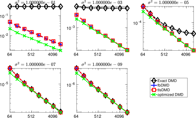
Figure 1: Example 1. This figure shows the mean Frobenius norm error (averaged over 1000 runs) in the reconstructed system matrix ${\mathbf{A}}$ as a function of the number of snapshots $m$ for various noise levels $\sigma^{2}$.

In Fig. 1, we plot the mean Frobenius norm error in the reconstructed system matrix (averaged over the trials) as a function of the number of snapshots for various noise levels. We see that, as in [9], the error in the exact DMD eventually levels off at the higher noise levels because of the bias in its eigenvalues. The other methods perform well, with the error decaying as the number of snapshots increases. The optimized DMD is shown to have an advantage over the fbDMD and tlsDMD in this measure primarily at the highest noise levels and with the fewest snapshots.

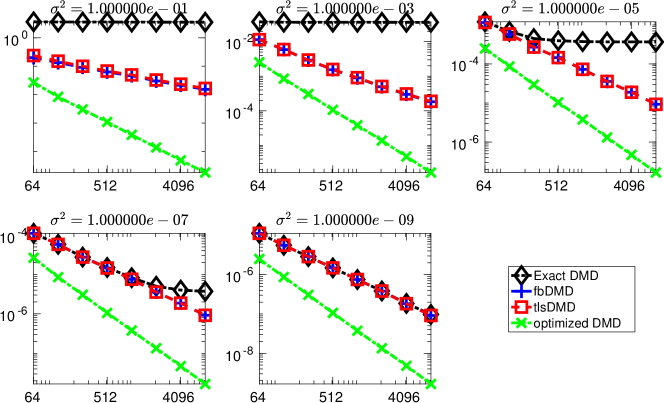
Figure 2: Example 1. This figure shows the mean $l^{2}$ error (averaged over 1000 runs) in the recovered eigenvalues of the system matrix ${\mathbf{A}}$ as a function of the number of snapshots $m$ for various noise levels $\sigma^{2}$.

Figure 2 contains plots of the $l^{2}$ norm error in the computed eigenvalues (averaged over the trials) as a function of the number of snapshots for various noise levels. Again, the error in the exact DMD eventually levels off at the lower noise levels because of the bias in its eigenvalues. The other methods perform well, with the error decaying as the number of snapshots increases. However, in this measure, the advantage of the optimized DMD is more pronounced. The error in the eigenvalues for the optimized DMD is lower than for the fbDMD and tlsDMD across all noise levels and is observed to decrease faster as the number of snapshots is increased.

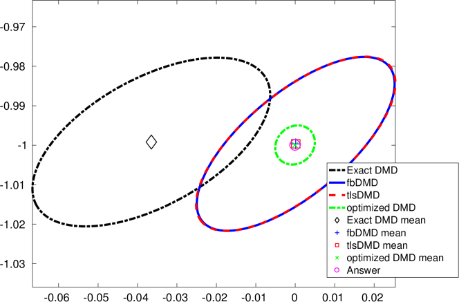
Figure 3: Example 1. This figure shows 95 percent confidence ellipses for the eigenvalue $i$ (based on 1000 runs) for the second-highest noise level $\sigma^{2}=10^{-3}$ and fewest snapshots $m=64$.

We plot 95 percent confidence ellipses (in the complex plane) for the eigenvalue $i$ for the second-highest noise level and fewest number of snapshots in Fig. 3. The bias in the exact DMD is evident, as the center of the ellipse is seen to be shifted into the left half-plane. The fbDMD and tlsDMD are seen to correct for this bias, but the spread of the optimized DMD eigenvalues is notably smaller.

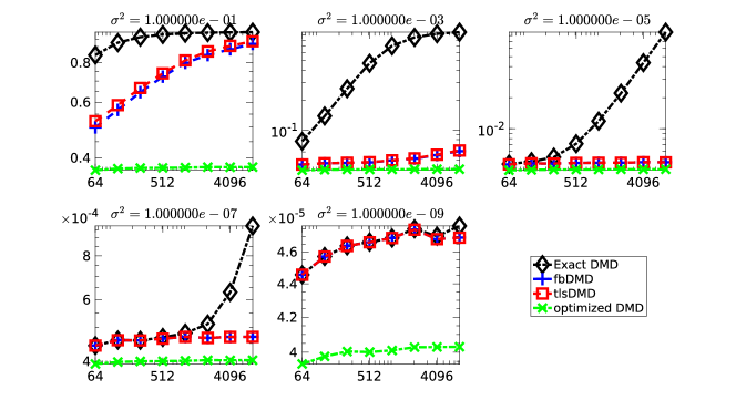
Figure 4: Example 1. This figure shows the mean Frobenius norm error (averaged over 1000 runs) of the reconstructed snapshots as a function of the number of snapshots $m$ for various noise levels $\sigma^{2}$.

In Fig. 4, we plot the mean error in the optimal reconstruction of the snapshots using the computed eigenvalues, see Eq. 70 for the definition of this error. The optimized DMD demonstrates an advantage across noise levels and number of snapshots used, though it is more pronounced at higher noise levels. Further, the error in the optimized DMD is seen to be relatively flat as the number of snapshots increases, which is to be expected. The reconstruction error increases for the other methods as the number of snapshots increases, particularly at the higher noise levels.

4.1.2 Example 2: measurement noise, hidden dynamics

In the case that a signal contains some rapidly decaying components it can be more difficult to identify the dynamics, particularly in the presence of sensor noise [9]. We consider a signal composed of two sinusoidal signals which are translating, with one growing and one decaying, i.e.

(72) $$z(x,t)=\sin(k_{1}x-\omega_{1}t)e^{\gamma_{1}t}+\sin(k_{2}x-\omega_{2}t)e^{\gamma_{2}t}\;,$$

where $k_{1}=1$, $\omega_{1}=1$, $\gamma_{1}=1$, $k_{2}=0.4$, $\omega_{2}=3.7$, and $\gamma_{2}=-0.2$ (these are the settings used in [9]). This signal has four continuous time eigenvalues given by $\gamma_{1}\pm i\omega_{1}$ and $\gamma_{2}\pm i\omega_{2}$. We set the domain of $x$ to be $[0,15]$ and use 300 equispaced points to discretize. For the time domain, we set $\Delta t=2\pi/(2^{9}-1)$ so that the largest number of snapshots we use, $m=2^{9}$, covers $[0,2\pi]$.

As before, we consider the effect of both the size of the noise, $\sigma$, and the number of snapshots, $m$, on the quality of the modes and eigenvalues obtained from various methods. We set the noise level to the values $\sigma^{2}=2^{-2},2^{-4},\ldots,2^{-10}$ and run tests with $m=2^{7},2^{8},2^{9}$ snapshots (the range of the number of snapshots is more limited for this problem by the exponential growth in the signal). For each noise level and number of snapshots, we compute the eigenvalues and modes of this system using the exact DMD, fbDMD, tlsDMD, and optimized DMD over 1000 trials (different draws of the vector ${\mathbf{g}}$). We compute the DMD for each of these methods with the data projected on the first 4 POD modes (the first 4 left singular vectors of the data matrix). For the optimized DMD, this means we are using the approximate algorithm, algorithm 3.

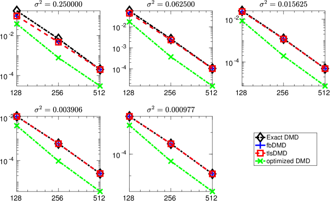
Figure 5: Example 2. This figure shows the mean $l^{2}$ error (averaged over 1000 runs) in the recovered dominant (growing) eigenvalues of the system as a function of the number of snapshots $m$ for various noise levels $\sigma^{2}$.

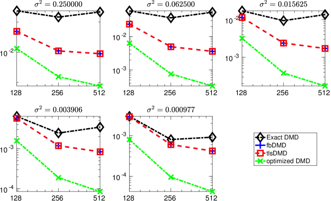
Figure 6: Example 2. This figure shows the mean $l^{2}$ error (averaged over 1000 runs) in the recovered hidden (shrinking) eigenvalues of the system as a function of the number of snapshots $m$ for various noise levels $\sigma^{2}$.

In Figs. 5 and 6, we plot the mean $l^{2}$ error (averaged over the trials) in the recovered dominant eigenvalues ($1\pm i$) and the recovered hidden eigenvalues ($-0.2\pm 3.7i$), respectively. For the dominant eigenvalues, the exact DMD, fbDMD, and tlsDMD perform similarly and the optimized DMD has lower error, up to an order of magnitude more accurate for some settings. For the hidden eigenvalues, the bias in the exact DMD is evident and it performs notably worse. It seems that the same phenomenon occurs in which the bias of the exact DMD causes these curves to level off prematurely. Of course, the signal for the hidden eigenvalues will eventually decay so much that there is no advantage in adding more snapshots. This is evident in these plots as the curves flatten out for all methods. Again, the optimized DMD has an advantage across noise levels and number of snapshots. Importantly, it appears that for some noise levels, the other methods won’t perform as well as the optimized DMD, even if you provide them with more snapshots.

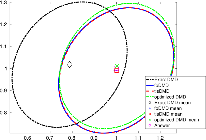
Figure 7: Example 2. This figure shows 95 percent confidence ellipses for one of the dominant eigenvalues (based on 1000 runs) for the highest noise level $\sigma^{2}=2^{-2}$ and fewest snapshots $m=128$.

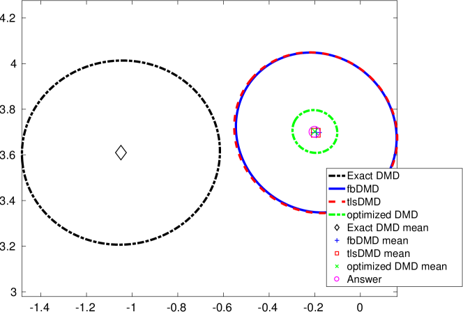
Figure 8: Example 2. This figure shows 95 percent confidence ellipses for one of the hidden eigenvalues (based on 1000 runs) for the highest noise level $\sigma^{2}=2^{-2}$ and fewest snapshots $m=128$.

We plot 95 percent confidence ellipses (in the complex plane) for the eigenvalues $1+i$ and $-0.2+3.7i$ in Figs. 7 and 8, respectively, for the highest noise level and fewest number of snapshots. The bias in the exact DMD is evident, as the center of the ellipse is seen to be shifted to the left for both eigenvalues. For the dominant eigenvalue ($1+i$), we see that the spread of the eigenvalues for the fbDMD, tlsDMD, and optimized DMD are similar and that all three of these methods correct for the bias. For the hidden eigenvalue ($-0.2+3.7i$), the fbDMD, tlsDMD, and optimized DMD all correct for the bias but the spread of the optimized DMD is notably smaller.

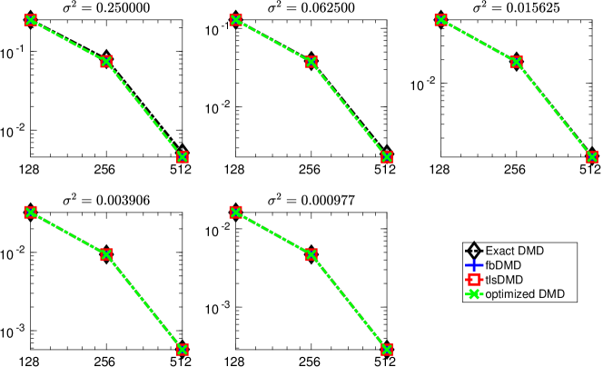
Figure 9: Example 2. This figure shows the mean Frobenius norm error (averaged over 1000 runs) of the reconstructed snapshots as a function of the number of snapshots $m$ for various noise levels $\sigma^{2}$.

In Fig. 9, we plot the mean error in the optimal reconstruction of the snapshots using the computed eigenvalues, see Eq. 70 for the definition of this error. In contrast with the periodic example, the error curves roughly coincide for all methods and the error decreases as the number of snapshots increases. This is likely a result of the fact that the growing modes dominate more and more as the system advances in time (when new snapshots are added, they come from later in the time series). It is interesting that the reconstruction error is only marginally better for the optimized DMD — this error is what the optimized DMD tries to minimize — but the recovered eigenvalues are significantly better.

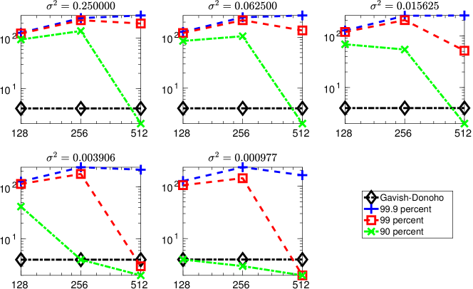
Figure 10: Example 2. This figure shows the mean estimated rank of the data (averaged over 1000 runs) using the Gavish-Donoho, 99.9 percent, 99 percent, and 90 percent hard-thresholds as a function of the number of snapshots $m$ for various noise levels $\sigma^{2}$.

Because the data in this example is in a high dimensional space relative to the rank of the dynamics, we must use some sort of truncation when computing the DMD (using any of the methods). For the comparisons above, we used the a priori knowledge we have of the system to always truncate at rank 4. When this a priori information is unavailable, it is sometimes necessary to determine an appropriate truncation from the data. In Fig. 10, we compare the hard-threshold (the number of singular values to keep) obtained from the Gavish-Donoho formula [11] with the hard-threshold obtained by keeping 99.9, 99, and 90 percent of the energy in the singular values. The Gavish-Donoho formula always produced 4 in our experiments, while the cut-offs based on keeping a certain percentage of the energy produced wildly different results depending on noise level and number of snapshots. The type of error in this example exactly satisfies the assumptions used to obtain the Gavish-Donoho formula; nonetheless, the performance of the formula is impressive in comparison with these other a posteriori methods.

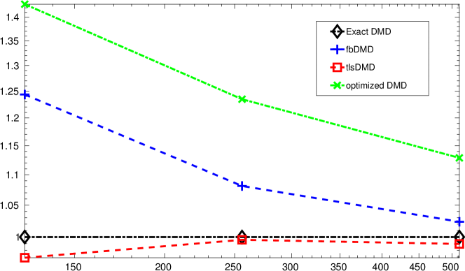
Figure 11: Example 2. This figure shows the mean run-time of the methods (averaged over 1000 runs) relative to the mean run-time for the exact DMD as a function of the number of snapshots $m$.

In Fig. 11, we plot the mean run-time of each method as you increase the number of snapshots, with the values normalized by the mean run-time of the exact DMD. We see that the optimized DMD indeed requires more computation than the other methods but that the increase is modest. For this example, the run-time is dominated by the SVD used for the truncation in each method. These values should be taken with a grain of salt, as they depend significantly on the quality of the implementation (and, for the optimized DMD, on the parameters sent to the optimization routine). Note that our implementation of the fbDMD checks every possible square root for the optimal answer, which is costly for larger systems.

4.1.3 Example 3: uncertain sample times, periodic system

For this example, we revisit the system of Example 1, Eq. 71, but introduce a different type of sampling error: uncertain sample times. Let ${\mathbf{z}}(t)$ be the solution of Eq. 71 with the initial condition ${\mathbf{z}}(0)=(1,0.1)^{\intercal}$. Let the snapshots be given by ${\mathbf{z}}_{j}={\mathbf{z}}((j+\sigma g_{j})\Delta t)$ with $\Delta t=0.1$, $\sigma$ a prescribed noise level, and ${\mathbf{g}}$ a vector whose entries are drawn from a standard normal distribution. Again, the continuous time eigenvalues of this system are $\pm i$ (this is how the optimized DMD computes eigenvalues) and the discrete time eigenvalues are $\exp(\pm\Delta ti)$. Intuitively, the methods should behave like they did for the sensor noise example (consider the Taylor series of ${\mathbf{z}}((j+\sigma g_{j})\Delta t)$ about ${\mathbf{z}}(j\Delta t)$) but there is a different structure to the noise here.

We consider the effect of both the size of the noise, $\sigma$, and the number of snapshots, $m$, on the quality of the modes and eigenvalues obtained from various methods. We set the noise level to the values $\sigma^{2}=2^{-2},2^{-4},\ldots,2^{-10}$ and run tests with $m=2^{6},2^{7},\ldots,2^{13}$ snapshots. For each noise level and number of snapshots, we compute the eigenvalues and modes of this system using the exact DMD, fbDMD, tlsDMD, and optimized DMD over 1000 trials (different draws of the vector ${\mathbf{g}}$).

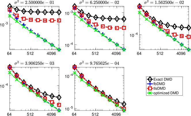
Figure 12: Example 3. This figure shows the mean Frobenius norm error (averaged over 1000 runs) in the reconstructed system matrix ${\mathbf{A}}$ as a function of the number of snapshots $m$ for various noise levels $\sigma^{2}$.

In Fig. 12, we plot the mean Frobenius norm error in the reconstructed system matrix (averaged over the trials) as a function of the number of snapshots for various noise levels. We see that, as in Example 1, the error in the exact DMD eventually levels off at the higher noise levels because of the bias in its eigenvalues. Surprisingly, this occurs for the tlsDMD as well, but at a lower error. The fbDMD and optimized DMD perform well, with the error decaying as the number of snapshots increases. The optimized DMD shows slight improvement over the fbDMD at the highest noise levels and with the fewest snapshots.

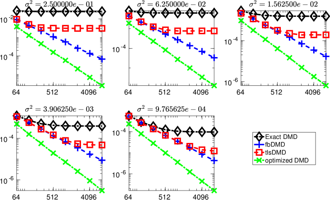
Figure 13: Example 3. This figure shows the mean $l^{2}$ error (averaged over 1000 runs) in the recovered eigenvalues of the system matrix ${\mathbf{A}}$ as a function of the number of snapshots $m$ for various noise levels $\sigma^{2}$.

Figure 13 contains plots of the $l^{2}$ norm error in the computed eigenvalues (averaged over the trials) as a function of the number of snapshots for various noise levels. Again, the error in the exact DMD eventually levels off at the lower noise levels because of the bias in its eigenvalues. We see similar behavior for the tlsDMD. The fbDMD and optimized DMD perform well, with the error decaying as the number of snapshots increases. However, in this measure, the advantage of the optimized DMD is more pronounced. The error in the eigenvalues for the optimized DMD is lower than for the fbDMD and tlsDMD across all noise levels and is observed to decrease faster as the number of snapshots is increased.

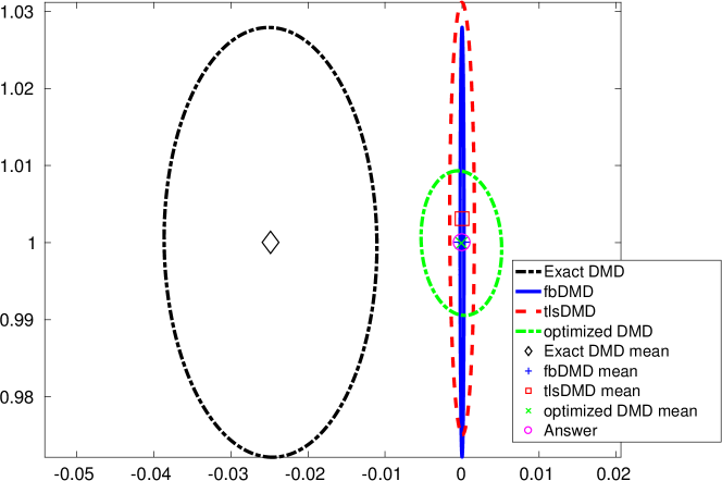
Figure 14: Example 3. This figure shows 95 percent confidence ellipses for the eigenvalue $i$ (based on 1000 runs) for the highest noise level $\sigma^{2}=2^{-2}$ and fewest snapshots $m=64$.

We plot 95 percent confidence ellipses (in the complex plane) for the eigenvalue $i$ for the highest noise level and fewest number of snapshots in Fig. 14. Again, the bias in the exact DMD is indicated by the fact that the ellipse is shifted into the left half-plane. Curiously, the tlsDMD displays a different type of bias, consistently overestimating the frequency of the oscillation. The fbDMD and optimized DMD are relatively bias-free, with the fbDMD having a smaller spread along the real axis and the optimized DMD having a smaller spread along the imaginary axis. We believe that the strong performance of the fbDMD here is rather intuitive: by averaging the forward and backward dynamics, the fbDMD should nearly cancel the noise we’ve introduced with the uncertain sample times.

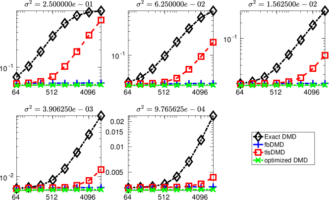
Figure 15: Example 3. This figure shows the mean Frobenius norm error (averaged over 1000 runs) of the reconstructed snapshots as a function of the number of snapshots $m$ for various noise levels $\sigma^{2}$.

In Fig. 15, we plot the mean error in the optimal reconstruction of the snapshots using the computed eigenvalues, see Eq. 70 for the definition of this error. The fbDMD and optimized DMD perform the best across noise levels and number of snapshots used, though the advantage is more pronounced at higher noise levels. The reconstruction error increases for the exact DMD and tlsDMD as the number of snapshots increases, particularly at the higher noise levels.

From the above, we see that uncertain sample times can produce errors in the computed DMD modes and eigenvalues which are qualitatively different from the errors produced by sensor noise. We believe that this source of error may be of interest when analyzing data collected by humans or historical data sets. When dealing with real data, it is clear how to perform sensitivity analysis for additive sensor noise: simply rerun the method for the data with sensor noise added. It is unclear how to perform sensitivity analysis for uncertain sample times using the exact DMD, fbDMD, or tlsDMD. Using the optimized DMD, such an analysis is again simple: rerun the method for the same data set while adding noise to the sample times that you send to the optimized DMD routine.

4.2 Example 4: Sea surface temperature data

For the final example, we consider a real data set: the “optimally-interpolated” sea surface temperature (OISST-v2, AVHRR only) data set from the National Oceanic and Atmospheric Administration (NOAA) [30, 6]. This is a data set of daily average ocean temperatures, with 1/4 degree resolution in latitude and longitude, for a total of about 700k grid points over the ocean. The temperatures are reported to four decimal digits. We considered two subsets of this data: 521 snapshots (10 years) spaced 7 days apart and 521 snapshots spaced randomly, with an average of 7 days apart, with each set starting on January 1st, 1982.

rank	$\rho_{DMD}$	$\rho_{tlsDMD}$	$\rho_{optDMD}$	$\rho_{POD}$
2	1.0446e-01	1.0447e-01	1.0437e-01	4.8298e-02
4	6.5921e-02	5.3714e-02	4.5387e-02	4.1057e-02
8	5.3453e-02	4.4864e-02	3.8655e-02	3.7276e-02
16	4.6376e-02	4.0935e-02	3.5443e-02	3.3905e-02
32	3.8045e-02	3.2955e-02	3.1733e-02	3.0039e-02
64	3.1939e-02	2.8125e-02	2.7884e-02	2.5879e-02
128	2.7792e-02	9.8115e-01	2.3751e-02	2.1195e-02

Table 1: Example 4. This table shows the relative residual of the best possible reconstruction using the eigenvalues obtained from the exact DMD, tlsDMD, and optimized DMD, as $\rho_{DMD}$, $\rho_{tlsDMD}$, and $\rho_{optDMD}$, respectively, for several different values of the reconstruction rank $r$. The value $\rho_{POD}$ is the relative norm of the residual when projecting the data onto $r$ POD modes and represents a rough lower bound on the relative residual for DMD modes.

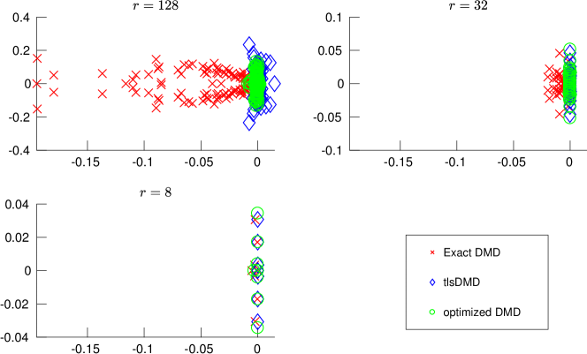
Figure 16: Example 4. We plot the eigenvalues obtained using the exact DMD, tlsDMD, and optimized DMD for various target ranks $r$.

When it comes to properly truncating this data set for the DMD, there are a number of complicating factors: the sensor noise is not simply additive white noise, the values have been interpolated, and the underlying dynamics are not linear. In particular, the assumptions used to obtain the Gavish-Donoho formula are not satisfied. In Table 1, we see that the error in the optimal reconstruction, using the eigenvalues for any of the methods, decreases weakly as you increase the rank of the system. This is largely driven by the slow decay in the singular values of the data matrix (compare the reconstruction quality for the optimized DMD with that obtained for POD modes). For the largest rank, $r=128$, the reconstruction error has actually increased for the tlsDMD. We will see that this is due to some spurious eigenvalues in the tlsDMD which correspond to an unreasonable amount of growth.

In Fig. 16, we produce scatter plots of the DMD eigenvalues obtained from the exact DMD, tlsDMD, and optimized DMD for various choices of the DMD rank $r$. Setting $r=128$ (this is close to the value $r=124$ obtained from the Gavish-Donoho formula), the exact DMD has a number of strongly decaying modes and there are some growing modes visible for the tlsDMD. There is not much agreement among the methods at this level. For $r=32$, the exact DMD and tlsDMD give more reasonable values and there is more agreement among the methods but still some significant discrepancy in the eigenvalues. For $r=8$, we see that all of the methods obtain similar eigenvalues. From the preceding, it is unclear how to choose the correct rank $r$ without a priori knowledge.

Coefficient	optimized DMD	tlsDMD	exact DMD
+1.5302e+04	+2.8122e+18	+Inf	+Inf
+9.8238e+02	-1.3565e+17	+Inf	+Inf
+9.7476e+02	-3.6530e+02	-3.6695e+02	-3.6767e+02
+9.7476e+02	+3.6530e+02	+3.6695e+02	+3.6767e+02
+2.3189e+02	-6.5046e+02	-5.0713e+02	-5.3827e+02
+2.3189e+02	+6.5046e+02	+5.0713e+02	+5.3827e+02
+2.1204e+02	-1.8261e+02	-1.8957e+02	-1.9056e+02
+2.1204e+02	+1.8261e+02	+1.8957e+02	+1.9056e+02
+1.3309e+02	-7.9859e+02	-8.1385e+02	-8.5878e+02
+1.3309e+02	+7.9859e+02	+8.1385e+02	+8.5878e+02
+1.1419e+02	-2.9084e+03	-4.2224e+03	-6.6036e+03
+1.1419e+02	+2.9084e+03	+4.2224e+03	+6.6036e+03
+6.6960e+01	+1.6955e+03	+1.9867e+03	+1.9270e+03
+6.6960e+01	-1.6955e+03	-1.9867e+03	-1.9270e+03
+4.8591e+01	-1.0973e+03	-1.5181e+03	-1.7531e+03
+4.8591e+01	+1.0973e+03	+1.5181e+03	+1.7531e+03

Table 2: Example 4. This table shows the wavelength (in days) for each eigenvalue computed using the exact DMD, tlsDMD, and optimized DMD, for the evenly spaced data with $r=16$. The optimized DMD wavelengths are ordered according to the magnitude of the corresponding spatial mode and the other wavelengths are chosen in the order which best matches the optimized DMD values.

Because this data set comes from temperature measurements over time, we know some of the wavelengths we should find in the data set. In particular, there should be a background mode with infinite wavelength and a mode corresponding to a tropical year (365.24 days). In Table 2, we see that these wavelengths are discovered by each DMD method. The tropical year wavelength recovered by the optimized DMD method (365.30 days) is remarkably close to the true value, particularly considering that the data is only provided to four decimal digits. We see that the second harmonic of this frequency, or a wavelength of half a tropical year, is also discovered by the DMD methods. The half-year wavelength from the optimized DMD (182.61 days) is again quite accurate (actual value 182.62 days).

even — $b$	uneven — $b$	even — $\lambda$	uneven — $\lambda$	projection
+1.5302e+04	+1.4465e+04	+2.8122e+18	-1.9361e+20	+9.9964e-01
+9.8238e+02	+5.4390e+02	-1.3565e+17	+4.3709e+17	+4.4502e-02
+9.7476e+02	+9.7456e+02	-3.6530e+02	-3.6526e+02	+9.9981e-01
+9.7476e+02	+9.7456e+02	+3.6530e+02	+3.6526e+02	+9.9981e-01
+2.3189e+02	+2.8990e+02	-6.5046e+02	-6.0671e+02	+8.6006e-01
+2.3189e+02	+2.8990e+02	+6.5046e+02	+6.0671e+02	+8.6006e-01
+2.1204e+02	+2.1168e+02	-1.8261e+02	-1.8259e+02	+9.9591e-01
+2.1204e+02	+2.1168e+02	+1.8261e+02	+1.8259e+02	+9.9591e-01
+1.3309e+02	+8.6639e+01	-7.9859e+02	-8.6279e+02	+8.7601e-01
+1.3309e+02	+8.6639e+01	+7.9859e+02	+8.6279e+02	+8.7601e-01
+1.1419e+02	+9.6051e+01	-2.9084e+03	-2.2726e+03	+7.6004e-01
+1.1419e+02	+9.6051e+01	+2.9084e+03	+2.2726e+03	+7.6004e-01
+6.6960e+01	+7.7304e+01	+1.6955e+03	+1.4850e+03	+8.0135e-01
+6.6960e+01	+7.7304e+01	-1.6955e+03	-1.4850e+03	+8.0135e-01
+4.8591e+01	+1.0787e+02	-1.0973e+03	-1.2015e+03	+7.5979e-01
+4.8591e+01	+1.0787e+02	+1.0973e+03	+1.2015e+03	+7.5979e-01

Table 3: Example 4. This table compares the wavelengths $\lambda$ obtained using the optimized DMD for each of the evenly spaced and randomly spaced data sets, with $r=16$. The wavelengths obtained from the evenly spaced data are ordered according to the magnitude of the corresponding spatial mode (the $b$ values) and the wavelengths for the randomly spaced data are chosen in the order which best matches the evenly spaced DMD values. In the last column, we report the cosine of the angle between the spatial mode from the evenly spaced data and the spatial mode from the randomly spaced data.

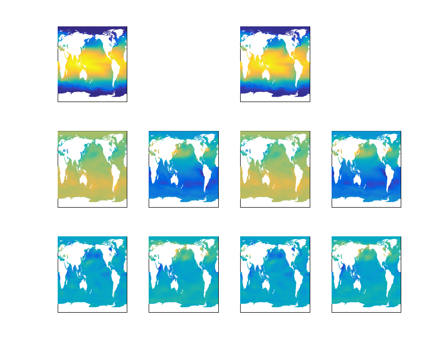
Figure 17: Example 4. We plot the spatial modes obtained using the optimized DMD for two different subsets of the data, one with evenly spaced snapshots (left two columns) and randomly spaced snapshots (right two columns). The top row corresponds to a static background mode, the middle row the real and imaginary parts of a mode with a one-year wavelength, and the bottom row the real and imaginary parts of a mode with a half-year wavelength.

One way to verify the eigenvalues obtained from the optimized DMD on the evenly spaced data set is to compare these with the eigenvalues from the randomly spaced data set. For $r=16$, we computed DMD eigenvalues and modes using the optimized DMD on each data set. The wavelengths corresponding to these eigenvalues are reported in Table 3. There is good agreement for the infinite, one year, and half-year wavelengths, and less-so for the others. Further, the spatial modes for these wavelengths are very similar. We measure this using the cosine of the angle between the corresponding spatial modes, which is near 1 in absolute value for the infinite, one year, and half-year wavelengths. Heatmaps of these modes are provided in Fig. 17. We find this to be a convincing confirmation of these wavelengths, which did not require a priori knowledge.

rank	$t_{DMD}$	$t_{tlsDMD}$	$t_{optDMD}$
2	2.7675e-01	2.7798e-01	1.3367e+00
4	4.3028e-01	3.6161e-01	1.1965e+00
8	7.1807e-01	3.6795e-01	1.0157e+00
16	6.7264e-01	3.8975e-01	1.6571e+00
32	1.0951e+00	1.2162e+00	4.7037e+00
64	2.1410e+00	1.5664e+00	1.6101e+01
128	5.4412e+00	3.4158e+00	3.0226e+01

Table 4: Example 4. The run time (excluding the SVD of the data used for projecting onto POD modes) for each method and various values of the rank $r$ on the evenly spaced data set.

Some basic timing info for these calculations is provided in Table 4. The time reported is the total time used by the algorithm, excluding the cost of the SVD used to project the data onto POD modes (the time for this calculation was 32 seconds). For ranks less than or equal to $r=32$, the optimized DMD costs only about 4 times as much as the other methods. For the largest rank, $r=128$, the optimized DMD is about a factor of 10 times more costly. Even then, the cost of the optimized DMD is roughly equal to the cost of the initial SVD. For larger $r$, the computational cost of the optimized DMD appears to increase like $r^{2}$, which is lower than the bound we expect based on the estimates in Section 3.

5 Conclusions and future directions

Based on the numerical experiments above, we believe that the optimized DMD is the DMD algorithm of choice for many applications. The resulting modes and eigenvalues are less sensitive to noise than those computed using the other DMD methods we tested and the optimized DMD overcomes the bias issues of the exact DMD. In some cases, the improvement over existing methods in robustness to noise is significant. For example 2, the optimized DMD algorithm is better able to capture the hidden dynamics than the other DMD methods, sometimes showing an order of magnitude improvement in the error. For the sea surface temperature data, example 4, the optimized DMD obtains modes which more accurately describe yearly patterns; indeed, the accuracy of the yearly and half-yearly wavelengths obtained by the optimized DMD is comparable with the accuracy of the data (the exact DMD and tlsDMD are an order of magnitude less accurate for these wavelengths).

Of course, these advantages come at a cost: computing the optimized DMD requires the solution of a nonlinear, nonconvex optimization problem. As noted above, it is unclear whether we have actually solved this optimization problem (globally) in our numerical experiments. The solutions we have obtained nonetheless represent improvements over existing DMD methods and the cost of the optimization algorithm is modest for the range of problem sizes considered above. We see in Fig. 11 that, for this problem size, the cost of the optimized DMD is only about 1.5 times that of the exact DMD in the worst case (as the number of snapshots increases, the cost of the projection onto POD modes begins to dominate the calculation, so the times for each method become closer to equal). For the larger climate example, the run time of the optimized DMD was about 6 times that of the exact DMD (for various values of the reconstruction rank $r$), see Table 4. This is a more significant cost increase, but even for the largest rank, $r=128$, the cost of the optimized DMD was roughly equal to that of the SVD required to project onto POD modes (this cost is left out of the values in Table 4). We should stress that these timings depend strongly on the implementation of the given algorithms and even the parameters sent to the optimization routine. The MATLAB implementation of algorithms 2 and 3 we prepared for these experiments is available online [3, 4].

The apparent efficiency of the optimized DMD algorithms is a result of the variable projection methods which have been developed for nonlinear least squares problems. Further, by rephrasing the problem as fitting exponentials to data, the optimized DMD also represents a more general method. It is no longer necessary to assume that the snapshots are evenly spaced in time.

There are a few different avenues available for future research. As mentioned above, the variable projection framework applies to a wide range of optimization problems and could therefore serve as the basis for an optimized DMD with the addition of a sparsity prior (see Section 2.2.4). Such a method could help side-step the problem of choosing the correct target rank a priori. Also mentioned above is the possibility of using a block Schur decomposition, as opposed to an eigendecomposition, in the definition of the DMD. This could potentially improve the ability of the DMD to stably approximate transient dynamics. Finally, a few new directions are available because the sample times need not be evenly spaced for the optimized DMD. As seen in miniature for the climate example, making use of arbitrary sample times allows for some interesting types of cross-validation (and indeed expands the number of possible cross-validation sets for a given set of snapshots). There is also the possibility of using incoherent time sampling (e.g. randomly spaced times) to detect high frequency signals using less data than implied by the Shannon sampling theorem.

References

- [1] A. Aravkin, D. Drusvyatskiy, and T. van Leeuwen, Variable projection without smoothness, arXiv preprint arXiv:1601.05011, (2016).
- [2] A. Y. Aravkin and T. Van Leeuwen, Estimating nuisance parameters in inverse problems, Inverse Problems, 28 (2012), p. 115016.
- [3] T. Askham, askhamwhat/dmd-varpro-paper-examples: optdmd figure generation, Mar. 2017, https://doi.org/10.5281/zenodo.439373, https://doi.org/10.5281/zenodo.439373.
- [4] T. Askham, duqbo/optdmd: optdmd v1.0.0, Mar. 2017, https://doi.org/10.5281/zenodo.439385, https://doi.org/10.5281/zenodo.439385.
- [5] S. Bagheri, Koopman-mode decomposition of the cylinder wake, Journal of Fluid Mechanics, 726 (2013), pp. 596–623.
- [6] V. Banzon, T. M. Smith, T. M. Chin, C. Liu, and W. Hankins, A long-term record of blended satellite and in situ sea-surface temperature for climate monitoring, modeling and environmental studies, Earth System Science Data, 8 (2016), pp. 165–176, https://doi.org/10.5194/essd-8-165-2016, http://www.earth-syst-sci-data.net/8/165/2016/.
- [7] B. M. Bell and J. V. Burke, Algorithmic differentiation of implicit functions and optimal values, in Advances in Automatic Differentiation, Springer, 2008, pp. 67–77.
- [8] K. K. Chen, J. H. Tu, and C. W. Rowley, Variants of dynamic mode decomposition: boundary condition, koopman, and fourier analyses, Journal of nonlinear science, 22 (2012), pp. 887–915.
- [9] S. T. Dawson, M. S. Hemati, M. O. Williams, and C. W. Rowley, Characterizing and correcting for the effect of sensor noise in the dynamic mode decomposition, Experiments in Fluids, 57 (2016), pp. 1–19.
- [10] N. B. Erichson and C. Donovan, Randomized low-rank dynamic mode decomposition for motion detection, Computer Vision and Image Understanding, 146 (2016), pp. 40–50.
- [11] M. Gavish and D. L. Donoho, The optimal hard threshold for singular values is , IEEE Transactions on Information Theory, 60 (2014), pp. 5040–5053.
- [12] G. Golub and V. Pereyra, Separable nonlinear least squares: the variable projection method and its applications, Inverse problems, 19 (2003), p. R1.
- [13] G. H. Golub and R. J. LeVeque, Extensions and uses of the variable projection algorithm for solving nonlinear least squares problems, in Proceedings of the 1979 Army Numerical Analsysis and Computers Conference, 1979, http://faculty.washington.edu/rjl/pubs/GolubLeVeque1979/index.html.
- [14] G. H. Golub and V. Pereyra, The differentiation of pseudo-inverses and nonlinear least squares problems whose variables separate, SIAM Journal on numerical analysis, 10 (1973), pp. 413–432.
- [15] G. H. Golub and J. H. Wilkinson, Ill-conditioned eigensystems and the computation of the jordan canonical form, SIAM review, 18 (1976), pp. 578–619.
- [16] N. Halko, P.-G. Martinsson, and J. A. Tropp, Finding structure with randomness: Probabilistic algorithms for constructing approximate matrix decompositions, SIAM review, 53 (2011), pp. 217–288.
- [17] M. S. Hemati, C. W. Rowley, E. A. Deem, and L. N. Cattafesta, De-biasing the dynamic mode decomposition for applied koopman spectral analysis, arXiv preprint arXiv:1502.03854, (2015).
- [18] M. Ilak and C. W. Rowley, Modeling of transitional channel flow using balanced proper orthogonal decomposition, Physics of Fluids, 20 (2008), p. 034103.
- [19] M. R. Jovanović, P. J. Schmid, and J. W. Nichols, Sparsity-promoting dynamic mode decomposition, Physics of Fluids, 26 (2014), p. 024103.
- [20] L. Kaufman, A variable projection method for solving separable nonlinear least squares problems, BIT Numerical Mathematics, 15 (1975), pp. 49–57.
- [21] J. N. Kutz, S. L. Brunton, B. W. Brunton, and J. L. Proctor, Dynamic mode decomposition: Data-driven modeling of complex systems, 2016.
- [22] K. Levenberg, A method for the solution of certain non-linear problems in least squares, Quarterly of applied mathematics, 2 (1944), pp. 164–168.
- [23] D. W. Marquardt, An algorithm for least-squares estimation of nonlinear parameters, Journal of the society for Industrial and Applied Mathematics, 11 (1963), pp. 431–441.
- [24] I. Mezic, Analysis of fluid flows via spectral properties of the Koopman operator, Annual Review of Fluid Mechanics, 45 (2013), pp. 357–378.
- [25] C. Moler and C. Van Loan, Nineteen dubious ways to compute the exponential of a matrix, SIAM review, 20 (1978), pp. 801–836.
- [26] K. M. Mullen, M. Vengris, and I. H. van Stokkum, Algorithms for separable nonlinear least squares with application to modelling time-resolved spectra, Journal of Global Optimization, 38 (2007), pp. 201–213.
- [27] D. P. O’leary and B. W. Rust, Variable projection for nonlinear least squares problems, Computational Optimization and Applications, 54 (2013), pp. 579–593.
- [28] M. Osborne, Nonlinear least squares—the levenberg algorithm revisited, The Journal of the Australian Mathematical Society. Series B. Applied Mathematics, 19 (1976), pp. 343–357.
- [29] V. Pereyra and G. Scherer, Exponential data fitting and its applications, Bentham Science Publishers, 2010.
- [30] R. W. Reynolds, T. M. Smith, C. Liu, D. B. Chelton, K. S. Casey, and M. G. Schlax, Daily high-resolution-blended analyses for sea surface temperature, Journal of Climate, 20 (2007), pp. 5473–5496.
- [31] C. W. Rowley, Model reduction for fluids, using balanced proper orthogonal decomposition, International Journal of Bifurcation and Chaos, 15 (2005), pp. 997–1013.
- [32] C. W. Rowley, I. Mezić, S. Bagheri, P. Schlatter, and D. S. Henningson, Spectral analysis of nonlinear flows, Journal of fluid mechanics, 641 (2009), pp. 115–127.
- [33] C. W. Rowley and D. R. Williams, Dynamics and control of high-reynolds-number flow over open cavities, Annu. Rev. Fluid Mech., 38 (2006), pp. 251–276.
- [34] C. W. Rowley, D. R. Williams, T. Colonius, R. M. Murray, and D. G. MacMynowski, Linear models for control of cavity flow oscillations, Journal of Fluid Mechanics, 547 (2006), p. 317.
- [35] A. Ruhe and P. Å. Wedin, Algorithms for separable nonlinear least squares problems, Siam Review, 22 (1980), pp. 318–337.
- [36] P. J. Schmid, Dynamic mode decomposition of numerical and experimental data, Journal of Fluid Mechanics, 656 (2010), pp. 5–28.
- [37] P. Shearer and A. C. Gilbert, A generalization of variable elimination for separable inverse problems beyond least squares, Inverse Problems, 29 (2013), p. 045003.
- [38] J. H. Tu, C. W. Rowley, D. M. Luchtenburg, S. L. Brunton, and J. N. Kutz, On dynamic mode decomposition: theory and applications, arXiv preprint arXiv:1312.0041, (2013).