HiFrames: High Performance Data Frames in a Scripting Language

Abstract

Data frames in scripting languages are essential abstractions for processing structured data. However, existing data frame solutions are either not distributed (e.g., Pandas in Python) and therefore have limited scalability, or they are not tightly integrated with array computations (e.g., Spark SQL). This paper proposes a novel compiler-based approach where we integrate data frames into the High Performance Analytics Toolkit (HPAT) to build HiFrames. It provides expressive and flexible data frame APIs which are tightly integrated with array operations. HiFrames then automatically parallelizes and compiles relational operations along with other array computations in end-to-end data analytics programs, and generates efficient MPI/C++ code. We demonstrate that HiFrames is significantly faster than alternatives such as Spark SQL on clusters, without forcing the programmer to switch to embedded SQL for part of the program. HiFrames is 3.6x to 70x faster than Spark SQL for basic relational operations, and can be up to 20,000x faster for advanced analytics operations, such as weighted moving averages (WMA), that the map-reduce paradigm cannot handle effectively. HiFrames is also 5x faster than Spark SQL for TPCx-BB Q26 on 64 nodes of Cori supercomputer.

1 Introduction

The rise of data science has led to the emergence of a wide variety of data analytics frameworks that support relational operations within a general purpose programming language. These frameworks can be roughly split into two categories - data frame packages and big data frameworks. Data frame packages in scripting languages, such as Python Pandas McKinney , R data frames rda , and Julia DataFrames jul [a] allow quick prototyping of data analytics algorithms. Because data frames are typically implemented as collections of their column arrays, they support standard array operations as well as relational query APIs. Scripting data frames have varying levels of integration with the language but all have the same performance limitations as the underlying scripting system. Data frame packages run sequentially and are limited in the amount of data they can process to what can fit in the memory of a single node.

An alternative approach is based on the map-reduce paradigm Zaharia et al. [2010]; Dean and Ghemawat [2008]; had ; Kornacker et al. [2015]; tez ; fli and distributed execution engines. Spark SQL Armbrust et al. [2015] and DryadLINQ Yu et al. [2008] provide examples of such systems. Big data frameworks allow fault-tolerant processing of large amounts of data on multiple nodes of a distributed system. But, they suffer from several limitations. First, they do not provide as seamless and efficient integration between relational and procedural operations as scripting data frame packages. Because relational operations are implemented by a separate sub-system via lazy evaluation, they cannot be efficiently integrated with arbitrary non-relational processing. Second, systems that rely on map-reduce paradigm cannot efficiently implement distributed computational patterns that go beyond map-reduce, such as scan or stencil. As a result, they can be prohibitively slow for advanced analytical operations, such as computing cumulative sums or moving averages. Finally, distributed execution via master-slave library approach is known to carry large overheads, as master node acts as a sequential bottleneck Totoni et al. .

In this paper, we introduce HiFrames in an effort to improve the programmability and performance of relational processing in analytics programs. HiFrames provides a set of scripting language extensions for structured data processing and a corresponding framework that can automatically parallelize and compile data analytics programs for distributed execution. Similar to data frame packages, HiFrames provides a data frame interface, supports smooth integration of relational and analytical processing and requires minimal typing. Similar to big data frameworks, HiFrames allows for distributed execution across large data sets. In addition, HiFrames optimizes across relational and non-relational data-parallel operations, supports flexible communication patterns and leverages the power of MPI/C++ to provide efficient and scalable distributed execution on small or large clusters.

HiFrames uses a novel compilation approach to generating efficient code for data frame operations. Traditionally, data frames are implemented as complex objects, such as, for example, arrays of arrays. This representation is necessary to support complex relational operations (join, aggregate) but limits optimization opportunities with array-based code. In HiFrames, each data frame column represented as a separate array variable and all data frame operations are expanded to work on individual arrays. This allows HiFrames to generate highly efficient code without overhead of object-based data frame representation. HiFrames also supports domain-specific relational optimizations, generalizing them for a case when program may contain both relational and non-relational operations.

HiFrames implementation is based on the Julia programming language. HiFrames leverages HPAT Totoni et al. to automatically extract parallelism based on the semantics of the program, distribute data between nodes based on heuristics about the data analytics domain and generate parallel code with highly efficient communication. HiFrames uses novel compilation techniques to implement data frame operations with minimal overhead and introduces domain-specific optimizations for relational operations. We compare performance of HiFrames with that of Python Pandas and Julia DataFrames, as examples of data frame packages, and Spark SQL, as the most recent and best performing instance of a distributed big data system, demonstrating significant performance advantages over both of these approaches.

This paper contributions are as follows:

• We present an end-to-end data analytics system that integrates relational data processing with array computations in a scripting language using a productive data frames API.

• We describe domain-specific compiler techniques to automatically parallelize data frame operations integrated in an array system.

• We present novel compiler optimization techniques that provide the equivalent of SQL query optimization in a general compilation setting.

• We demonstrate significant performance improvements over other frameworks that support relational data analytics in a general programming language. For individual relational operations, HiFrames outperforms both Python (Pandas) and Spark SQL by 3.5x-177x. For advanced analytics operations that require complex communication patterns, HiFrames is 1,000-20,000x faster than Spark SQL. Finally, for TPCx-BB Q25, Q26 benchmarks Ghazal et al. [2013] HiFrames is 3-10x faster than Spark SQL and provides good scalability.

2 Background

In this section, we provide an overview of data frames and the existing approaches used by existing big data systems for data analytics. In addition, we describe the HPAT and ParallelAccelerator systems, which we use as infrastructure for HiFrames.

2.1 Data Frames

Data analytics requires mathematical operations on arrays, as well as relational operations on structured data. Hence, scripting languages such as Python, R, and Julia provide data frame abstractions McKinney ; rda ; jul [a]. A data frame is a table or a two-dimensional array-like structure. Columns in a data frame are named and may have heterogeneous types but all the columns in a given data frame have identical length. In addition, columns of data frames can be used in computation as regular arrays. Data frames are similar to tables in a traditional relational database, but are designed to provide high-level APIs such that domain experts (e.g. data scientists and statisticians) can use them easily in procedural programs.

Data frames are typically implemented as libraries, e.g. DataFrames.jl in Julia jul [a] and Pandas in Python McKinney , that provide relational operations. These operations include filtering rows based on conditions, joining data frames, and aggregating column values based on a key column. Furthermore, they provide advanced analytics operations (e.g. moving averages) and are tightly integrated with the underlying array system to support array computations.

Data frames are essential for big data analytics systems. The popularity of data frames among data scientists confirms this fact: Pandas in Python and DataFrames.jl in Julia are among the top popular computational packages pyp ; jul [b]. Furthermore, users of the DataFrame API of Spark SQL increased by 153% in 2016 spa [b], even though its interface is more restrictive than the SQL API.

2.2 Big Data Systems

Current big data systems such as Apache Hadoop had and Apache Spark Zaharia et al. [2010] enable productive programming for clusters using the MapReduce paradigm Dean and Ghemawat [2008]. The system provides high-level data-parallel operations such as map and reduce, which are suitable for data processing, but hides the details of parallel execution. These systems are implemented as distributed runtime libraries, where a master node schedules tasks on slave nodes.

However, these systems sacrifice performance for productivity and are known to be orders of magnitude slower than low-level hand-written parallel programs Jha et al. [2014]. This is despite performance being the most important aspect for many users; 91% of Spark users cited performance among the most important aspects for them in a Spark survey, more than any other aspect spa [a]. Significant development effort has not found a solution (Spark has over 1000 contributors spa [b]) since the problem is fundamental: The distributed runtime library approach does not follow basic principles of parallel computing such as avoiding sequential bottlenecks (the master node is inherently a sequential bottleneck). Furthermore, the runtime task scheduling overhead is wasteful, since most analytics programs can be statically parallelized Totoni et al. .

Moreover, these systems are typically implemented in languages such as Java and Scala that can have significant overheads Maas et al. [2015]; Lion et al. [2016]; Ousterhout et al. [2015]. The reason is that providing various data structures as part of API and implementing a complex distributed library is much easier in these object-oriented languages. In addition, protections and facilities of a sandbox like Java Virtual Machine (JVM) helps development and maintenance of these complex systems. Hence, JVM overheads can be attributed to the distributed library approach, but our compiler approach naturally avoids them due to code generation.

2.3 Spark SQL

Spark is a big data processing framework based on the Map-Reduce programming model Dean and Ghemawat [2008], which is implemented as a master-slave distributed library. It provides high-level operations such as map and reduce on linearly distributed collections called Resilient Distributed Datasets (RDDs) Zaharia et al. [2012]. Spark SQL is a SQL query processing engine built on top of Spark that allows structured data processing inside Spark programs (as SQL strings) Armbrust et al. [2015]. It compiles and optimizes SQL to Java byte code that runs on top of RDD APIs for distributed execution. Spark SQL also provides data frame APIs in Python and Scala that go through the same compiler pipeline. However, these functional APIs are restrictive for advanced analytics (our target domain). For example, they cannot provide multiple aggregations, and are restricted to simple expressions of data frame columns inside filter and aggregate operations. In summary, Spark SQL has various disadvantages for data scientists:

• It requires writing part of the program in SQL which hurts productivity and is not type-safe.

• It inherits the inefficiencies of distributed libraries such as master-slave bottleneck and scheduling overheads.

• It cannot provide parallel operations that do not fit in map-reduce paradigm such as moving averages efficiently (Section 5).

In this paper, Spark SQL is our baseline for distributed execution since it is the state-of-the-art distributed system that can support end-to-end data analytics programs.

2.4 HPAT Overview

We build HiFrames on top of High Performance Analytics Toolkit (HPAT), which demonstrated that it is possible to achieve productivity and performance simultaneously for array computations in data analytics and machine learning Totoni et al. . HPAT performs static compilation of high-level scripting programs into high performance parallel codes using domain-specific compiler techniques. By generating scalable MPI/C++ programs, this approach enables taking advantage of compiler technologies (e.g. vectorization in C compilers), as well as other HPC technologies (e.g. optimized collective communication routines of MPI). In this work, we integrate data frames with HPAT to create a complete solution for data analytics that is both productive and efficient. Automatic parallelization for distributed-memory machines is known to be a difficult problem Kennedy et al. [2007], but HPAT can perform this task using a domain-specific data flow algorithm (which we extend). Since HPAT avoids distributed library overheads such as runtime scheduling and master-slave coordination, it is orders of magnitude faster than other systems such as Spark Zaharia et al. [2010]. Furthermore, HPAT can generate parallel code to call existing HPC libraries such as HDF5 Folk et al. [1999], ScaLAPACK Choi et al. [1992], and Intel^® DAAL Int . Section 4 includes more details about the compilation pipeline of HPAT.

HPAT is built on top of ParallelAccelerator compiler infrastructure, which is designed to extract parallel patterns from high-level Julia programs. These patterns include map, reduce, Cartesian map, and stencil. For example, ParallelAccelerator identifies array operations such as -, !, log, exp, sin, etc. as having map semantics. Then, ParallelAccelerator generates a common “parallel for” or parfor representation that allows a unified optimization framework for all the parallel patterns.

2.5 Fault Tolerance

Fault tolerance is a major concern for large, unreliable clusters. Spark provides fault tolerance using lineage of operations on RDDs, while HPAT provides automatic minimal checkpoint/restart Dongarra et al. [2015]. HiFrames does not provide fault tolerance for failures during relational operations, since we found the portion of our target programs with relational operations to be significantly shorter than the mean time between failure (MTBF) of moderate-sized clusters. Moreover, recent studies have shown that in practice most clusters consist of 30-60 machines which is a scale at which fault tolerance is not a big concern Ren et al. [2013]. In essence, the superior performance of HiFrames helps users avoid paying the fault tolerance overheads by keeping execution times short (as Section 5 demonstrates). On the other hand, iterative machine learning algorithms could require fault tolerance, which HPAT provides. Spark SQL also does not provide fault tolerance for relational operations.

3 HiFrames Syntax

Operations	Julia	SQL	HiFrames
Projection	v = df[:id]	select id from t	v = df[:id]
Filter	df2 = df[df[:id].<100,:]	select * from table where id<100	df2 = df[:id<100]
Join	rename!(df2,:id,:cid) df3 = join(df1, df2, on=:id)	select * from t1 join t2 on t1.id=t2.cid	df3 = join(df1, df2, :id==:cid)
Aggregate	df2 = by(df,:id, df -> DataFrame( xc = sum(df[:x].<1.0), ym = mean(df[:y])))	select count(case when x<1.0 then 1 else null) as xc, avg(y) as ym from t group by id	df2 = aggregate(df1, :id, :xc = sum(:x<1.0), :ym = mean(:y))
Concatenation	df3 = [df1; df2]	select * from t1 union all select * from t2	df3 = [df1; df2]
Cumulative Sum	cumsum(df[:x])	select sum(x) over (rows between unbounded preceding and current row) from t1	cumsum(df[:x])
Simple Moving Average (SMA)	for i in 2:size(x,1)-1 A[i] = (df[:x][i-1]+    df[:x][i]+df[:x][i+1])/3.0 end	select avg(x) over (rows between 1 preceding and 1 following) from t1	A = stencil(x-> (x[-1]+x[0]+x[1])/3.0,df[:x])
Weighted Moving Average (WMA)	for i in 2:size(x,1)-1 A[i] = (df[:x][i-1]+    df[:x][i]+2*df[:x][i+1])/4.0 end	select (lag(x,1) over (rows between 1 preceding and 1 following) + 2*x + lead(x,1) over (rows between 1 preceding and 1 following))/4.0 from t1	A = stencil(x-> (x[-1]+2*x[0]+x[1])/4.0,df[:x])

Table 1: Examples demonstrating relational and analytics API of Julia (DataFrames.jl), SQL and HiFrames.

The goal of HiFrames is to provide high-level data frame abstractions that are flexible, type-safe, and integrate seamlessly with array computations. We make our APIs similar to Julia’s DataFrames.jl to facilitate adoption, but provide syntactic sugars based on the patterns we have observed in data analytics programs.

3.1 Data Frames API

Input data frames:

To specify the schema and read a data frame, we extend the DataSource construct of HPAT, which is used for reading input data. For example, the following code reads a data frame with three columns from an HDF5 file:

⬇

df = DataSource(DataFrame{:id=Int64, :x=Float64,

:y=Float64}, HDF5, "/data/data.hdf5")

The first argument is the schema of the data frame. Similar to DataFrames.jl, Julia’s symbols (e.g. :id) are used for referring to column names. Each column’s type is also specified. The equivalent code in Spark (Python) follows:

⬇

schema = StructType(\

[StructField("id",LongType(),True),\

StructField("x",DoubleType(),True),\

StructField("y",DoubleType(),True)])

df = spark.createDataFrame(data, schema)

Projection:

One can use columns of HiFrames as arrays which is equivalent to the projection relational operation (see example in second row of Table 1).

Filter:

HiFrames allows filtering data frames using a conditional expression as shown in the third row of Table 1. This example filters all the row whose “id” column value is less than 100. For convenience, the user can refer to columns by just their names and use simple mathematical operators instead of element-wise operators (see desugaring in Section 4.1). However, any array expression that results in a boolean array can be used, and referring to any array in the program (including columns of other data frames) is allowed.

Join:

HiFrames provides the join operation as shown in the fourth row of Table 1. Note that unlike Julia’s DataFrames.jl, our API allows different column names as keys for the two input tables.

Aggregate:

HiFrames provides “split-and-combine” operations through a flexible aggregate() syntax, which is demonstrated in the fifth row of Table 1.Instead of the anonymous lambda syntax of Julia’s DataFrames.jl, we extend the aggregate() call to accept column assignment expressions shown as syntactic sugar.

Concatenation:

HiFrames provides vertical concatenation of data frames with the same schema, demonstrated in the fifth row of Table 1.

Cumulative sum:

Cumulative sum (cumsum) calculates the sequence of partial sums over an array. It is an example of built-in analytics functions of scripting languages HiFrames provides (sixth row of Table 1). In SQL, it requires defining a window from the first row of the table to the current row being processed.

Simple Moving Average (SMA):

Simple Moving Average (SMA) is a data smoothing technique where for each value an average using neighboring values is calculated (sixth row of Table 1). Julia does not provide a specific syntax for SMA; Julia users typically write these operations as for loops since Julia compiles loops to native code. However, Python (Pandas) provides SMA using rolling windows:

⬇

A = df1[’x’].rolling(3,center=True).mean()

SQL requires defining a window and using the built-in avg() function. HiFrames provides one-dimensional stencil API to support moving averages, which improves productivity and allows parallelization.

Weighted Moving Average (WMA):

Weighted Moving Average (WMA) is similar to SMA, except that the user provides the weights for the average operation. Again, Julia requires a loop, while HiFrames handles WMA using stencils. Python (Pandas) provides WMA by accepting a user lambda for rolling windows:

⬇

A = df1[’x’].rolling(3,center=True).

apply(lambda x: (x[0]+2*x[1]+x[2])/4)

SQL provides lag() and lead() functions to access neighboring rows in a window using relative indices.

3.2 Example

Consider the following example data analytics program written using HiFrames, which is inspired by TPCx-BB Q26 benchmark Ghazal et al. [2013]:

⬇

@acc hiframes function customer_model(min_count,

num_centroids, iterations, file_name)

store_sales = DataSource(DataFrame{:s_item_sk=Int64,

:s_customer_sk=Int64}, HDF5, file_name)

item = DataSource(DataFrame{:i_item_sk=Int64,

:i_class_id=Int64}, HDF5, file_name)

sale_items = join(store_sales, item,

:s_item_sk==:i_item_sk)

c_i_points = aggregate(sale_items, :s_customer_sk,

:c_i_count = length(:s_item_sk),

:id1 = sum(:i_class_id==1),

:id2 = sum(:i_class_id==2),

:id3 = sum(:i_class_id==3))

c_i_points = c_i_points[:c_i_count>min_count]

c_i_points[:id3] = (c_i_points[:id3]-

mean(c_i_points[:id3]))/var(c_i_points[:id3])

samples = transpose(typed_hcat(Float64,

c_i_points[:c_i_count], c_i_points[:id1],

c_i_points[:id2], c_i_points[:id3])

model = HPAT.Kmeans(samples, num_centroids, iterations)

return model

end

This program performs market segmentation where it builds a model of separation for customers based on their purchase behavior. It reads store_sales and item data frames from file and joins them. Then, it forms training features based on the number of items each customer bought in total and in different classes. The program also filters the customers that bought less than a minimum number. Feature scaling is used for column :id3 based on its mean and variance (var). The next step is matrix assembly where the training matrix is formed: The call typed_hcat is a standard Julia operation where arrays are concatenated horizontally (including type conversion). Also, the matrix is transposed since Julia has column major layout and features need to be on the same column. Finally, K-means clustering algorithm is called to train the model. Note that this program is simplified and there could be much more mathematical operations (array computations) such as data transformations and feature scaling. Furthermore, the user might write a custom machine learning algorithm instead of calling a library. The equivalent Spark SQL version is about 2$\times$ longer and includes a SQL string for relational operations.

4 Compiling Data Frames

Figure 1: Compiler pipeline of HiFrames. For data frame support, we added DataFrame-Pass and extended Macro-Pass, Domain-Pass, Distributed-Pass, and CGen routines.

In this section, we describe HiFrames’s compiler implementation. HiFrames uses a novel dual representation approach: all columns are individual arrays in the AST which allows Julia and HPAT to optimize the program. However, HiFrames uses data frame metadata when necessary for relational transformations and optimizations. Figure  2 shows the initial code of a running example to illustrate the transformations of the HiFrames compiler pipeline.

⬇

df = DataSource(DataFrame{:id=Int64, :x=Float64,

HDF5, "data.hdf5")

df2 = aggregate(df, :id, :c = sum(:x<1.0))

Figure 2: Running example HiFrames source code.

⬇

Expr(:meta, (:df->((:id,Int64), (:x,Float64)), :df2->((:id,Int64), (:c,t1))))

_df_id = DataSource(Int64, "id", HDF5, "data.hdf5")

_df_x = DataSource(Int64, "x", HDF5, "data.hdf5")

expr_arr1 = _df_x .< 1.0

t1 = typeof(sum(expr_arr1))

arg_arrs_in = [_df_id, _df_x]

arg_arrs_out = HiFrames.API.aggregate(arg_arrs_in, :id, [(expr_arr1, sum)])

_df2_id::Vector{Int64} = arg_arrs_out[1]

_df2_c::Vector{t1} = arg_arrs_out[2]

Figure 3: Running example after Macro-Pass.

⬇

size1 = get_h5_size("id", "data.hdf5")

_df_id = alloc(Int64, size1)

_df_x = alloc(Float64, size1)

h5read(_df_id, "id", "data.hdf5", size1)

h5read(_df_x, "x", "data.hdf5", size1)

expr_arr1 = map(.<, _df_x)

Expr(:aggregate, :df, :df2, (expr_arr1, sum))

Figure 4: Running example after Domain-Pass.

⬇

// allocations, read

MPI_Comm_size(MPI_COMM_WORLD, &npes);

H5Dopen2(...);

size1 = H5Sget_simple_extent_ndims(space_id_2);

_df_id = new int64_t[size1/npes];

H5Sselect_hyperslab(...);

H5Dread(...);

// same alloc, read calls for _df_x

expr_arr1 = new bool[size1/npes];

for(int i=0; i<size1/npes; i++) {

expr_arr1[i] = (_df_x[i]<1.0);

}

for(int i=0; i<size1/npes; i++) {

int pe_id = _df_id[i]%npes;

send_count[pe_id]++;

}

MPI_Alltoall(send_count,...);

for(int i=0; i<size1/npes; i++) {

// pack data in buffers for different processors

}

MPI_Alltoallv(temp_df_id,send_count, recv_df_id,...);

MPI_Alltoallv(temp_df_x,send_count, recv_df_x,...);

for(int i=0; i<recv_df_id.size(); i++) {

// aggregate using hash table

int64_t key = recv_df_id[i];

int write_ind = agg1_table[key];

_df2_c[write_ind] += expr_arr1[i];

}

Figure 5: Running example output C code.

Figure 1 provides an overview of the compiler pipeline. For data frame support, we added DataFrame-Pass and extended Macro-Pass, Domain-Pass, and Distributed-Pass. We also added code generation routines for relational operations in CGen.

4.1 Macro-Pass

Macro-Pass is called at the macro stage and is responsible for desugaring HiFrames operations to make sure Julia can compile the program. In addition, the types of all variables should be available to the Julia compiler for complete type inference. Here, we desugar data frame operations into regular array operations and function calls, and annotate variables with types using domain knowledge. In general, each data frame column is a regular array in the AST, but data frame metadata is included to enable relational operations and optimizations. The output of the Macro-Pass of our running example is shown in Figure  3.

Input data frames:

HiFrames desugars read operations for data frames into separate DataSource() calls for each column:

⬇

df_name = DataSource(DataFrame{:c1=<c1_type>,

:c2=<c2_type>, ...}, f_typ, file_path)

⬇

# assert length(_df_c1)==length(_df_c2)

Expr(:meta, (:df->((:id,Int64), (:x,Float64)))

_df_c1 = DataSource(<c1_type>, "c1", f_typ,file_path)

_df_c2 = DataSource(<c2_type>, "c2", f_typ,file_path)

...

Each column is an array but various metadata for the data frame is inserted in the metadata section of the AST (Expr(:meta) node in Julia). In addition, columns of the data frame are set to have the same length, which enables many array optimizations such as fusion. Furthermore, data frame column references are desugared to the underlying array (df[:id] to _df_id).

Filter:

HiFrames desugars filter operations into regular function calls on arrays. Since the number of columns of data frames is variable, HiFrames packs the columns into an array of arrays as follows:

⬇

df2 = df1[e(:c1, ...)]

⬇

Expr(:meta, (:df1->((:c1,T1), (:c2,T2)...), :df2->((:c1,T1), (:c2,T2)...)))

# replace column references of e to underlying arrays

e = ast_walk(replace_column_refs, e)

# convert scalar operations of e to element-wise operations

e = ast_walk(replace_opr_vector, e)

expr_arr = e

# n is number of columns of df1 which is constant

arg_arrs_in = Array(Array, n)

arg_arrs_in[1] = _df1_c1

arg_arrs_in[2] = _df1_c2

...

arg_arrs_out = HiFrames.API.filter(expr_arr, arg_arr_in)

_df2_c1::Vector{T1} = arg_arrs_out[1]

_df2_c2::Vector{T2} = arg_arrs_out[2]

...

For the translation of relational operations such as filter, HiFrames reads metadata of the involved data frame from metadata. For example, the types of output columns are assigned using the metadata information available from the input data frame. This desugaring method ensures that Julia can compile the generated code and perform complete type inference.

Join:

Join desugaring is similar to filter, except that there are two inputs data frames and the join expression should be specified. Currently, we support inner join on equal keys but relaxing this limitation is straightforward.

Aggregate:

Similar to filter, aggregate expressions are translated to replace scalar operations with element-wise counterparts and to replace column references with underlying arrays. However, the type of the output columns cannot be determined at the macro stage easily. Therefore, we generate dummy calls that apply the reduction functions on expression arrays to find the output type. Furthermore, for each output column, the expression array and the reduction function, which form a tuple, are passed as inputs to the aggregate function call. The aggregation key is also passed as input.

⬇

df2 = aggregate(df1, :c1, :c4=f1(e1(:c2,...)),

:c5=f2(e2(:c3,...)),

...)

⬇

Expr(:meta, (:df1->((:c1,T1), (:c2,T2)...), :df2->((:c1,t1), (:c4,t2)...)))

# replace column references of e1,e2,... to underlying arrays

# convert scalar operations of e1,e2,... to element-wise operations

expr_arr1 = e1

expr_arr2 = e2

...

# dummy call to get type of f1 output on expr_arr1

t1 = typeof(f1(expr_arr1))

t2 = typeof(f2(expr_arr2))

...

arg_arrs_out = HiFrames.API.aggregate(:c1, arg_arrs_in, [(expr_arr1, f1), (expr_arr2, f2), ...])

_df2_c1::Vector{t1} = arg_arrs_out[1]

_df2_c4::Vector{t2} = arg_arrs_out[2]

...

Concatenation:

HiFrames desugars union of data frames into vertical concatenation of columns (Julia’s vcat() call) after making sure schemas are equal.

4.2 Domain-Pass

Julia then translates the code to its internal representation and performs type inference. Next, the Domain-Pass encapsulates relational operations into their own AST nodes so that HPAT and ParallelAccelerator can be applied. The output of the Domain-Pass of our running example is shown in Figure  4.

⬇

Expr(:filter, expr_arr, out_df, in_df,...)

Expr(:join, key_arrs, out_df, in_df1, in_df2,...)

Expr(:aggregate, key_arr, out_df, in_df, expr_arrs, reduction_funcs,...)

Domain-Pass also simplifies the AST by removing all the unnecessary code generated after Julia compilation. For example, we remove the array of arrays variables used for passing data frames and the related packing/unpacking code generated.

Since HiFrames transforms relational operations into fully-fledged AST nodes, the optimizations of ParallelAccelerator and HPAT can transparently work with relational operations as well. For example, ParallelAccelerator dead code elimination will remove unused columns (column pruning) using the knowledge of the whole program, while Spark SQL performs column pruning only within the SQL context.

Moreover, Domain-Pass can perform pattern matching for common patterns of analytics workloads (before the structure is lost in later passes). For example, we match the transpose(typed_hcat()) pattern, since it is used for machine learning matrix assembly (see example of Section 3.2). HiFrames replaces the original code with a call to HiFrames.API.transpose_hcat(), which has an optimized code generation routine in the backend (HiFrames extension of CGen). We found this optimization to be significant for this step (not presented in this paper).

After Domain-Pass, we call the Domain-IR pass of ParallelAccelerator, which is responsible for normalizing the AST for further analysis. We insert the DataFrame-Pass after Domain-IR since some analyses, such as liveness analysis, are only available after this normalization.

4.3 DataFrame-Pass: Relational Optimizations

DataFrame-Pass is responsible for optimizing relational operations. Relational databases and other SQL systems such as Spark SQL usually optimize queries using a query tree and applying various rule-based transformations repeatedly. However, HiFrames receives some of the optimizations implemented in SQL systems for “free” by design. For example, the Julia compiler performs constant folding and common subexpression elimination and there is no need for HiFrames to implement them. In addition, ParallelAccelerator performs advanced optimizations such as loop fusion and intermediate array elimination. However, some optimizations are specific to relational operations and are not handled by general compilers. Performing these optimizations is challenging in a general program AST since relational operations of HiFrames are spread across the AST. For example, there could be array computation or sequential code between two relational nodes that need to be transformed.

We address this challenge in DataFrame-Pass by using the following heuristic-based approach. Similar to traditional databases, DataFrame-Pass starts by constructing a query tree of operations. However, unlike databases, this tree includes only relational operations while other nodes in the AST are ignored at this stage. The root node of the tree is the output data frame and each internal node corresponds to a relational operator. The leaf nodes represent the input data frames. Similar to databases, DataFrame-Pass then traverses the tree and checks the rules to find the transformations that can be applied. However, we need to make sure a transformation is valid for the full program before applying it since the query tree is only a partial view. For example, a column of a data frame could be used in array computations between two relational operations, and their transformation could change the result of the computation. To make sure a transformation does not change the semantics of the program, we use liveness analysis to find and inspect potential references to the columns of the involved data frames in any node that can be executed between the involved operators. Currently, we perform relational transformations within basic blocks only, since our use cases do not require transformations across control flow. Extending this pass to handle control flow is straightforward (e.g. make sure the earlier relational node is in a dominant block with respect to the later node).

We use this approach to implement the push predicate through join Hellerstein and Stonebraker [1993] optimization, which we found to be the most important for our current workloads. This optimization is potentially applicable when the output table of a join operation is filtered based only on the attributes of an input table. In this case, the input table can be filtered instead, which can reduce the cost of the join operation substantially by decreasing the data size. Figure 6 illustrates an example program before and after the transformation (6(a)), and the corresponding before and after trees (6(b) and 6(c)).

⬇

# customer dataframe has columns :id, :phone

# order dataframe has columns :customerId, :amount

cust_ord = join(customer, order, :id==:customerId)

...

cust_ord = cust_ord[:amount>100.0]

⬇

# is transformed to the equivalent of:

order2 = order[:amount>100.0]

...

cust_ord = join(customer, order2, :id==:customerId)

(a)

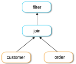
(b)

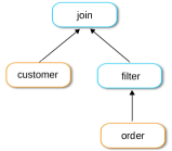
(c)

Figure 6: (a) Example program before and after push predicate through join transformation (b) Unoptimized tree (c) Optimized tree

After DataFrame-Pass, Parallel-IR is called which lowers computations into parfor nodes and performs more optimizations such as loop fusion.

4.4 Distributed-Pass

Parallelization for distributed-memory architectures is performed in Distributed-Pass. The first step is distribution analysis for arrays and parfor nodes to determine which arrays and computations should be parallelized. HPAT uses a heuristic-based data flow approach where distribution methods form a meet-semilattice. In a fixed-point iteration algorithm, the distribution method of each array and parfor is updated using domain-specific inference rules (i.e. transfer functions) for each node in the AST. The default distribution (top element of the semilattice) is one-dimensional block distribution (1D_BLOCK), which means all processors have equal chunks of data except possibly the last processor. However, the distribution can change all the way to replication (REP).

We extend the inference rules to support relational operations. Similar to other inference rules of HPAT, we use domain knowledge for developing these new rules. For example, all input and output arrays of an aggregate operation should be replicated if any of them is replicated, which makes the aggregate operation sequential. This is essentially assigning the meet of the distributions of the arrays to all of them.

However, the output arrays of relational operations need extra attention. Even though the input arrays could have one-dimensional block distribution, the output chunks can have variable length since the output size is data dependent. For example, filtering a data frame in parallel could result in different number of rows on different processors. This is an issue since some operations such as the distributed machine learning algorithms HPAT provides require 1D_BLOCK distribution for their input arrays. One could rebalance the data frames after every relational operation but this can be very costly. The best approach is to rebalance only when necessary, which we achieve using a novel technique.

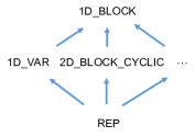
Figure 7: HiFrames extends the meet-semilattice of HPAT distributions with 1D_VAR to support relational operations.

To achieve this, we extend the meet-semilattice of distributions with a new one-dimensional variable length (1D_VAR) distribution. Figure 7 illustrates the new meet-semilattice. The transfer functions for output arrays of relational operations could be written as follows:

$dist[out\_arrs]={\small\texttt{\text{1D\_VAR}}}\wedge dist[in\_arr1]\wedge dist[in\_arr2]...$

Furthermore, we allow 1D_VAR as input to operations that require 1D_BLOCK during analysis. However, we generate a rebalance call in the AST right before these operations.

This technique allows having multiple parallel patterns in a program simultaneously and takes full advantage of the meet-semilattice of Figure 7. For example, one could use linear algebra algorithms that require two-dimentional block cyclic distribution along with relational operations, and generate data distribution conversions only when necessary. This is not possible with distributed libraries like Spark and Hadoop, since they have one-dimensional partitioning hard-coded in the system. Evaluation of this feature is left for future work.

4.5 Backend Code Generation in CGen

We extend CGen with code generation routines for relational operations. The output of this pass for our running example is shown in Figure  5. Operations such as filter do not require communication by taking advantage of our 1D_VAR distribution approach (Section 4.4). On the other hand, aggregate and join require data shuffling since rows with the same key need to be on the same processor for these operations (currently using hash partitioning). We use MPI_Alltoallv() collective communication routine of MPI to perform data shuffling. However, since MPI requires the amount of data to be known for each call, we use an initial MPI_Alltoall() operation for processors to coordinate the number of elements that will be communicated. Optimizing and tuning communication operations is left for future work. After data shuffling, join and aggregate operations are performed using standard algorithms. We use sort-merge for join, with Timsort Peters as the sorting algorithm. Aggregation is done using a hash table.

We add code generation routines for analytics operations as well. For example, cumsum generates loops for local partial sums and MPI_Exscan for the required parallel scan communication. Furthermore, stencils of HiFrames generate near neighbor communication and the associated border handling. To overlap communication and computation, non-blocking communication is used (MPI_Isend, MPI_Irecv and MPI_Wait).

Being able to take advantage of HPC technologies such as MPI collective communication routines give a significant advantage to our approach. This helps taking advantage of decades of development in the HPC domain. On the other hand, the Spark SQL approach requires building components such as shuffle collective on top of a distributed library like Spark, which can have significant overheads, increases development cost, and increases system complexity substantially.

5 Evaluation

In this section, we evaluate and compare the performance of analytics workloads on Spark SQL and HiFrames. While Spark is a highly optimized production system with over 1000 contributors spa [b], HiFrames is currently a research prototype without significant performance tuning effort. Nevertheless, performance comparison provides valuable insight about the two approaches.

We use a local 4-node cluster for evaluation (144 total cores). Each node has two sockets, each equipped with an Intel^®Xeon^®E5-2699 v3 processor (18-core “Haswell” architecture). The memory capacity per node is 128GB. The nodes are connected through an Infiniband network. We use Spark 2.0.1 for comparison which is the latest release at the time of this study. It is configured to take advantage of all of system memory and the Infiniband network. The cluster software includes Julia 0.5 compiled with Intel^®C++ Compiler 17, Intel^®MPI 2017 configured with DAPL communication stack, and Python 3.5.2 (Anaconda 4.1.1 distribution).

(a) Relational Operations (HiFrames is 3.6$\times$-70$\times$ faster than Spark SQL)

(b) Advanced Analytics Operations (HiFrames is 11$\times$-15781$\times$ faster than Spark SQL)

Figure 8: Performance of relational and analytics operations in various systems. Please note the logarithmic scale.

Basic Relational Operations:

We compare the performance of various systems that provide data frame API for the basic relational operations: filter, join, and aggregate. The input tables have an integer key field and two floating point numbers. The datasets are randomly generated from uniform distribution to avoid load balance issues. Dataset sizes are large enough to demonstrate parallel execution while making sure sequential systems (Python and Julia) do not run out of memory. Input tables to filter, join, and aggregate operations have 2 billion, 0.5 million, and 256 million rows, respectively.

Figure 8(a) demonstrates that HiFrames is 177$\times$, 21$\times$, and 3.5$\times$ faster than Python (Pandas) for filter, join, and aggregate, respectively. Furthermore, HiFrames is 3.8$\times$, 3.6$\times$, and 70$\times$ faster than Spark SQL. The choice of Spark interfaces does not affect our comparison significantly for these benchmarks. For these experiments, Spark SQL is expected to perform its best since the cluster is small and the master-slave bottleneck does not affect performance significantly. Furthermore, the benchmarks only involve simple operations that are easy to handle in Spark SQL backend compiler and are expected to be fast. Moreover, the parallel algorithms for these operations fit reasonably well with the map-reduce paradigm of Spark. Nevertheless, HiFrames is significantly faster since it uses HPC technologies instead of relying on a distributed library. Overall, the higher performance of HiFrames enables interactive analytics for data scientists using a small local cluster, since the execution times are in few seconds range for queries with few operations.

The results for the filter benchmark provide insights about the trade-off between generality and performance in these systems. Data frames of Python (Pandas) accept any expression evaluating to Boolean array for filtering data frames. However, the expression is not evaluated insides the optimized backend of Pandas and it can be slow. On the other hand, Spark only allows simple expressions with hard-coded operations on the data frame’s columns (e.g. df[‘id’]<100). These expressions evaluate to a class of type “Column” which is used for code generation in Spark SQL backend. HiFrames provides best of both worlds using an end-to-end compiler approach. It allows general array expressions as well as high performance execution simultaneously.

Figure 8(a) also demonstrates that parallel execution of aggregate in Spark SQL is slower than Python and Julia, while HiFrames achieves significant (but relatively small) speedup. The reason is that the communication overheads are more dominant for this operation, and using faster communication software stack is important. Note also that these relational operations are data-intensive and one cannot expect to keep all the processor cores busy, since memory bandwidth often becomes bottleneck.

Advanced Analytics Operations:

We compare the performance of various systems for cumulative summation (cumsum), simple moving average (SMA), and weighted moving average (WMA), which are common analytics operations (Section 3). The input table has 256 million rows but the operation is run on a single column. Figure 8(b) demonstrates that HiFrames is 11$\times$, 837$\times$, and 15781$\times$ faster than Python (Pandas) for cumsum, SMA, and WMA, respectively. In Python, SMA is significantly faster than WMA since SMA is run in the optimized backend of Pandas whereas WMA requires the user to pass a function that applies the weights. Again, this highlights the trade-off between performance and flexibility in current systems, while the end-to-end compiler approach of HiFrames avoids this issue.

Furthermore, HiFrames is 1330$\times$, 15500$\times$, and 20356$\times$ faster than Spark SQL. These operations are fundamentally challenging for Spark SQL since they require communication operations other than the ones (e.g. reduction) that are supported in map-reduce frameworks. Cumulative summation requires a scan (partial reductions) communication operation while moving averages require near neighbor exchanges. Since HiFrames is not limited to Spark, it can generate the appropriate communication calls (e.g. MPI_Exscan). On the other hand, Spark SQL gathers all the data on a single executor (core) and performs the computation sequentially. This results in data spill to disk even with the relatively modest dataset size used, due to excessive memory consumption of Spark.

User-defined functions (UDFs):

The two language design of Spark SQL has significant performance implications for many programs. Data scientists often need custom operations which can be written in the host language using Spark SQL’s UDF interface (similar to database systems). These UDFs can slow down the program significantly because Spark SQL only compiles and inlines its own hardcoded operations (e.g. +, *, exp, …). On the other hand, the end-to-end compiler approach of HiFrames naturally avoids this problem.

⬇

# Spark SQL no-UDF version

df = spark.sql("SELECT id AS id, SUM(2*x) AS sx, SUM(2*y) AS sy FROM points GROUP BY id")

# Spark SQL UDF version

spark.udf.register("myudf",lambda x:2*x,DoubleType())

df = spark.sql("SELECT id AS id, SUM(myudf(x)) AS sx, SUM(myudf(y)) AS sy FROM points GROUP BY id")

⬇

# no-UDF version

df = aggregate(df, :id, :sx = sum(2*:x),

:sy = sum(2*:y))

# UDF version

myudf = x->2*x

df = aggregate(df, :id, :sx = sum(myudf(:x)),

:sy = sum(myudf(:y)))

Figure 9: Spark SQL and HiFrames versions of UDF performance benchmark.

We evaluate the performance impact of UDFs in Spark SQL and HiFrames using a simple benchmark we designed for this purpose. For each system, we use a version with a UDF and a version without UDFs. Figure 10 illustrates the performance impact of using different versions in Spark SQL for Python and Scala interfaces and in HiFrames. The UDF version in Spark SQL is 24% slower with Python interface and 46% slower with Scala interface. However, the performance difference is negligible in HiFrames since the generated codes are identical.

Figure 10: Overhead of UDFs in Spark SQL and HiFrames. Using UDFs results in significant slowdown in Spark SQL since there are two languages

(a) Q26

(b) Q25

(c) Q05

Figure 11: Performance of TPCx-BB benchmarks in Spark SQL and HiFrames.

5.1 TPCx-BB Benchmarks

To evaluate programs with multiple relational operations working together, we use three benchmarks of TPCx-BB (BigBench) Ghazal et al. [2013], which is designed to evaluate the performance big data systems for analytics queries. We use Q05, Q25, and Q26 benchmarks since they are tasks that include various stages from loading and transforming data to building training matrices and calling machine learning algorithms. We use the default data generator in the suite Rabl et al. [2011]. To focus on relational performance, we exclude data load time and machine learning algorithm execution times. The original benchmarks were written for Apache Hive but we ported them to Spark SQL since Spark SQL is shown to be significantly faster Armbrust et al. [2015]. Even though we target scripting languages, we use the Scala/SQL interface for performance evaluation to observe the best performance of Spark. In addition, to enable uniform comparison across different problem sizes, we disable an optimization in Spark where tables smaller than a threshold are broadcast for join operations (spark.sql.autoBroadcastJoinThreshold=-1). This optimization is also not used in HiFrames. Note that since these benchmarks are designed for SQL systems, Spark SQL is able to optimize them easily, while they are stress tests for HiFrames.

Figure 11(a) compares the performance of Spark SQL and HiFrames for Q26 benchmark of TPCx-BB, demonstrating that HiFrames is 3$\times$ to 7$\times$ faster than Spark. One can conclude that HiFrames is capable of optimizing relational programs effectively in comparison to a SQL system. Furthermore, HiFrames is even faster since it employs a compiler and HPC technologies rather than relying on a distributed library.

Figure 11(b) compares the performance of Spark SQL and HiFrames for Q25 benchmark of TPCx-BB and demonstrates that HiFrames is 5$\times$ to 10$\times$ faster than Spark SQL. The gap is wider for this benchmark partially because it requires more computationally expensive operations (e.g. counting distinct values in aggregate) that benefit from low-level code generation of HiFrames.

Figure 11(c) compares the performance of Spark SQL and HiFrames for Q05 benchmark of TPCx-BB. This benchmark is challenging since it involves a join on a large table with highly skewed data. Hence, hash partitioning results in high load imbalance among processors which is a well-known problem in the parallel database literature DeWitt et al. [1992]; Xu et al. [2008]; Walton et al. [1991]. Spark SQL throws an error for scale factors greater than 50 since an internal sorting data structure runs out of memory. HiFrames throws an error for scale factor 400 only. The reason is a limitation in current MPI implementations where the data item counts cannot be more than $2^{32}$. Since load imbalance is well-studied in the HPC domain, HiFrames could take advantage of existing HPC technologies to address this problem. For example, HiFrames could generate code for Charm++ which includes advanced load balancing capabilities Acun et al. [2014] and naturally provides the virtual processor approach, which is proposed in the parallel database literature DeWitt et al. [1992]. The implementation of this feature is left for future work.

Strong Scaling:

We compare scalability of Spark SQL and HiFrames for large-scale distributed-memory machines using Cori (Phase I) supercomputer at NERSC COR . Each node has two Intel Xeon E5-2698 v3 processors (2$\times$16 cores) and 128GB of memory. Spark 2.0.0 is provided on Cori. Figure 12 demonstrates the strong scaling of Q26 benchmark from one to 64 nodes (32 to 2048 cores). We use scale factor 1000 dataset for this experiment, where the larger input table has 1.2 billion rows. Note that Spark crashes on settings with fewer than eight nodes because of resource limitations. The figure demonstrates that execution time of HiFrames decreases using more nodes up to 64 nodes, while Spark SQL is slower on 64 nodes compared to 16 nodes. Hence, HiFrames is 5$\times$ faster than Spark SQL on 64 nodes. The fundamental scalability limitation of Spark is due to its master-slave approach where the master becomes a sequential bottleneck Totoni et al. .

Figure 12: Scaling of Q26 in Spark SQL and HiFrames.

6 Related Work

HiFrames is the first compiler-based system for data frames that automatically parallelizes relational operations and tightly integrates with array computations. Hence, this work is related to areas such automatic parallelization, SQL embedding and big data processing.

Automatic Parallelization and Distribution:

Automatic parallelization is extensively studied in the literature Fonseca et al. [2016]; Tavarageri et al. [2015]; Bondhugula [2013], especially in the context of High Performance Fortran (HPF) Kennedy et al. [2007]; Adve et al. [1998]. Typically, arrays in such systems are aligned to a template of infinite virtual processors and then distributed based on heuristics. The computation is then distributed based on the owner-computes rule. For example, Kennedy and Kremer Kennedy and Kremer [1998] proposed a framework where the program is divided into phases (loop-nests) and all possible alignment-distribution pairs are found for each phase. Then, performance models are used to evaluate various layout and remapping costs. Finally, 0-1 integer programming is used to evaluate all possible layout and remapping combinations for the whole program, which is an NP-complete problem. However, auto-parallelization proved not to be practical because the compiler analysis was too complex and the generated programs significantly underperformed hand-written parallel programs Kennedy et al. [2007]. HPAT solved the auto-parallelization problem for scripting array programs in the data analytics and machine learning domain by exploiting domain knowledge Totoni et al. . We extend HPAT by integrating data frames and extending HPAT’s parallelization to relational operations. For example, we integrate a new parallelization method in its semilattice of parallelism methods (Section 4.4). Distributed Multiloop Language (DMLL) presents a new parallel IR and various transformations for heterogeneous platforms Brown et al. [2016]. However, DMLL starts from an explicitly parallel program and only includes simple parallelism inference for intermediate values. Nevertheless, some of their transformations could be used in HiFrames for operations such as filter and aggregate, which is left for future work.

Distributed Library Approach:

A common approach in previous work is building a SQL subsystem on top of a distributed library, such as Spark SQL Armbrust et al. [2015] on top of Spark Zaharia et al. [2010] and DryadLINQ Yu et al. [2008] on top of Dryad Isard et al. [2007]. These systems require writing relational code in SQL or a SQL-like DSL, which is executed on top of the distributed library. This approach has two main drawbacks for our target domain. First, there is no tight integration with array computations in the rest of the program. Second, the SQL subsystem inherits the fundamental performance limitations of these distributed libraries such master-slave and runtime scheduling overheads (see Section 2.2). HiFrames avoids these issues by providing data frame abstractions that are tightly integrated with array computations, and are compiled to efficient parallel code.

Language Integrated Queries:

The first and most straightforward method of accessing relational databases in a program was through the use of embedded SQL strings. However, this approach has problems with type-safety, error checking and security McClure and Kruger [2005]; Maier [1990]. Hence, language integrated queries have a long history  Breazu-Tannen et al. [1992] and is still an area of active research Cheney et al. [2013b]; McClure and Kruger [2005]; Maier [1990]; Meijer et al. [2006]. For example, Microsoft LINQ provides a DSL that is equivalent to SQL and is integrated in .NET languages Meijer et al. [2006]. Even though their target domain is different, future work could potentially apply some of LINQ’s transformations in HiFrames. Language integrated queries are particularly popular in functional languages  Ellis ; Suzuki et al. [2016]; Hibino et al. ; Cheney et al. [2013a] with their focus on type safety since integration allows queries to undergo compile-time type checking. Moreover, in some cases, these systems make it impossible by construction to create invalid SQL on the backend. Finally, these systems tend not to support data frames as such because their data stores are row-oriented rather than column oriented.

7 Conclusion and Future Work

This paper introduced HiFrames, which a compiler-based end-to-end data analytics framework that integrates array computations and relational operations seamlessly, and generates efficient parallel code. We presented HiFrames’s API, and the compiler techniques that make it possible. Our evaluation demonstrated superior performance of HiFrames compared to alternative systems.

HiFrames opens various research directions. More compiler optimizations across array computations and relational operations need to be explored. In addition, generating faster parallel code and using HPC techniques such as MPI/OpenMP hybrid parallelism could result in significant improvements. Moreover, HiFrames could potentially allow more complex data analytics programs that need to be investigated.

References

- [1] Cori Supercomputer at NERSC. http://www.nersc.gov/users/computational-systems/cori/.
- [2] Intel Data Analytics Acceleration Library. https://software.intel.com/en-us/intel-daal/.
- [3] Apache Flink: Scalable Batch and Stream Data Processing. https://flink.apache.org/.
- [4] Hadoop: Open-Source Implementation of MapReduce. http://hadoop.apache.org/.
- jul [a] Julia’s DataFrames, a. https://github.com/JuliaStats/DataFrames.jl.
- jul [b] Julia Package Ecosystem Pulse. http://pkg.julialang.org/pulse.html/, b.
- [7] PyPI Ranking. http://pypi-ranking.info/alltime/.
- [8] R project for statistical computing. http://www.r-project.org.
- spa [a] Apache Spark Survey 2015 Report. http://go.databricks.com/2015-spark-survey/, a.
- spa [b] Apache Spark Survey 2016 Report. http://go.databricks.com/2016-spark-survey/, b.
- [11] The Tez Project. http://tez.apache.org/.
- Acun et al. [2014] B. Acun, A. Gupta, N. Jain, A. Langer, H. Menon, E. Mikida, X. Ni, M. Robson, Y. Sun, E. Totoni, L. Wesolowski, and L. Kale. Parallel Programming with Migratable Objects: Charm++ in Practice. SC, 2014.
- Adve et al. [1998] V. Adve, G. Jin, J. Mellor-Crummey, and Q. Yi. High performance fortran compilation techniques for parallelizing scientific codes. In Supercomputing, 1998.SC98. IEEE/ACM Conference on, 1998.
- Armbrust et al. [2015] M. Armbrust, R. S. Xin, C. Lian, Y. Huai, D. Liu, J. K. Bradley, X. Meng, T. Kaftan, M. J. Franklin, A. Ghodsi, and M. Zaharia. Spark SQL: Relational data processing in Spark. In SIGMOD, 2015.
- Bondhugula [2013] U. Bondhugula. Compiling affine loop nests for distributed-memory parallel architectures. In 2013 SC - International Conference for High Performance Computing, Networking, Storage and Analysis (SC), 2013.
- Breazu-Tannen et al. [1992] V. Breazu-Tannen, P. Buneman, and L. Wong. Naturally embedded query languages. 1992.
- Brown et al. [2016] K. J. Brown, H. Lee, T. Rompf, A. K. Sujeeth, C. De Sa, C. Aberger, and K. Olukotun. Have abstraction and eat performance, too: Optimized heterogeneous computing with parallel patterns. In CGO, 2016.
- Cheney et al. [2013a] J. Cheney, S. Lindley, and P. Wadler. A practical theory of language-integrated query. In Proceedings of the 18th ACM SIGPLAN International Conference on Functional Programming, ICFP ’13, 2013a.
- Cheney et al. [2013b] J. Cheney, S. Lindley, and P. Wadler. A practical theory of language-integrated query. ACM SIGPLAN Notices, 48(9):403–416, 2013b.
- Choi et al. [1992] J. Choi, J. J. Dongarra, R. Pozo, and D. W. Walker. Scalapack: A scalable linear algebra library for distributed memory concurrent computers. In Frontiers of Massively Parallel Computation, 1992., Fourth Symposium on the, pages 120–127. IEEE, 1992.
- Dean and Ghemawat [2008] J. Dean and S. Ghemawat. MapReduce: simplified data processing on large clusters. Communications of the ACM, 2008.
- DeWitt et al. [1992] D. J. DeWitt, J. F. Naughton, D. A. Schneider, and S. Seshadri. Practical skew handling in parallel joins. University of Wisconsin-Madison. Computer Sciences Department, 1992.
- Dongarra et al. [2015] J. Dongarra, T. Herault, and Y. Robert. Fault tolerance techniques for high-performance computing. In Fault-Tolerance Techniques for High-Performance Computing. Springer, 2015.
- [24] T. Ellis. Opaleye. https://github.com/tomjaguarpaw/.
- Folk et al. [1999] M. Folk, A. Cheng, and K. Yates. HDF5: A file format and I/O library for high performance computing applications. In Proceedings of Supercomputing, volume 99, pages 5–33, 1999.
- Fonseca et al. [2016] A. Fonseca, B. Cabral, J. Rafael, and I. Correia. Automatic parallelization: Executing sequential programs on a task-based parallel runtime. International Journal of Parallel Programming, 44(6):1337–1358, 2016.
- Ghazal et al. [2013] A. Ghazal, T. Rabl, M. Hu, F. Raab, M. Poess, A. Crolotte, and H.-A. Jacobsen. BigBench: Towards an industry standard benchmark for big data analytics. In SIGMOD, 2013.
- Hellerstein and Stonebraker [1993] J. M. Hellerstein and M. Stonebraker. Predicate migration: Optimizing queries with expensive predicates. In SIGMOD. ACM, 1993.
- [29] K. Hibino, S. Murayama, S. Yasutake, S. Kuroda, and K. Yamamoto. Haskell Relational Record. http://khibino.github.io/haskell-relational-record/.
- Isard et al. [2007] M. Isard, M. Budiu, Y. Yu, A. Birrell, and D. Fetterly. Dryad: Distributed data-parallel programs from sequential building blocks. In EuroSys, New York, NY, USA, 2007.
- Jha et al. [2014] S. Jha, J. Qiu, A. Luckow, P. Mantha, and G. C. Fox. A tale of two data-intensive paradigms: Applications, abstractions, and architectures. In 2014 IEEE International Congress on Big Data, pages 645–652. IEEE, 2014.
- Kennedy and Kremer [1998] K. Kennedy and U. Kremer. Automatic data layout for distributed-memory machines. ACM Trans. Program. Lang. Syst., 20(4), July 1998. ISSN 0164-0925.
- Kennedy et al. [2007] K. Kennedy, C. Koelbel, and H. Zima. The rise and fall of high performance fortran: An historical object lesson. In Proceedings of the Third ACM SIGPLAN Conference on History of Programming Languages. ACM, 2007.
- Kornacker et al. [2015] M. Kornacker, A. Behm, V. Bittorf, T. Bobrovytsky, C. Ching, A. Choi, J. Erickson, M. Grund, D. Hecht, M. Jacobs, et al. Impala: A modern, open-source SQL engine for Hadoop. In CIDR, 2015.
- Lion et al. [2016] D. Lion, A. Chiu, H. Sun, X. Zhuang, N. Grcevski, and D. Yuan. Don’t get caught in the cold, warm-up your JVM: Understand and eliminate JVM warm-up overhead in data-parallel systems. In OSDI. USENIX Association, 2016.
- Maas et al. [2015] M. Maas, T. Harris, K. Asanović, and J. Kubiatowicz. Trash day: Coordinating garbage collection in distributed systems. In HotOS. USENIX Association, May 2015.
- Maier [1990] D. Maier. Advances in database programming languages. chapter Representing Database Programs As Objects, pages 377–386. ACM, 1990. ISBN 0-201-50257-7.
- McClure and Kruger [2005] R. A. McClure and I. H. Kruger. SQL DOM: compile time checking of dynamic SQL statements. In ICSE, 2005.
- [39] W. McKinney. pandas: a Foundational Python Library for Data Analysis and Statistics.
- Meijer et al. [2006] E. Meijer, B. Beckman, and G. Bierman. LINQ: Reconciling object, relations and XML in the .NET framework. In SIGMOD, New York, NY, USA, 2006. ACM.
- Ousterhout et al. [2015] K. Ousterhout, R. Rasti, S. Ratnasamy, S. Shenker, and B.-G. Chun. Making sense of performance in data analytics frameworks. In 12th USENIX Symposium on Networked Systems Design and Implementation (NSDI 15). USENIX Association, 2015.
- [42] T. Peters. Timsort description. https://svn.python.org/projects/python/trunk/Objects/listsort.txt. Accessed: November 2016.
- Rabl et al. [2011] T. Rabl, M. Frank, H. M. Sergieh, and H. Kosch. A data generator for cloud-scale benchmarking. In Proceedings of the Second TPC Technology Conference on Performance Evaluation, Measurement and Characterization of Complex Systems, TPCTC’10. Springer-Verlag, 2011.
- Ren et al. [2013] K. Ren, Y. Kwon, M. Balazinska, and B. Howe. Hadoop’s adolescence: An analysis of hadoop usage in scientific workloads. Proc. VLDB Endow., 2013.
- Suzuki et al. [2016] K. Suzuki, O. Kiselyov, and Y. Kameyama. Finally, safely-extensible and efficient language-integrated query. In Proceedings of the 2016 ACM SIGPLAN Workshop on Partial Evaluation and Program Manipulation, PEPM ’16, 2016.
- Tavarageri et al. [2015] S. Tavarageri, B. Meister, M. Baskaran, B. Pradelle, T. Henretty, A. Konstantinidis, A. Johnson, and R. Lethin. Automatic cluster parallelization and minimizing communication via selective data replication. In High Performance Extreme Computing Conference (HPEC), 2015 IEEE, 2015.
- [47] E. Totoni, T. A. Anderson, and T. Shpeisman. HPAT: High Performance Analytics with Scripting Ease-of-Use. https://arxiv.org/abs/1611.04934/.
- Walton et al. [1991] C. B. Walton, A. G. Dale, and R. M. Jenevein. A taxonomy and performance model of data skew effects in parallel joins. In VLDB, volume 91, pages 537–548, 1991.
- Xu et al. [2008] Y. Xu, P. Kostamaa, X. Zhou, and L. Chen. Handling data skew in parallel joins in shared-nothing systems. In SIGMOD. ACM, 2008.
- Yu et al. [2008] Y. Yu, M. Isard, D. Fetterly, M. Budiu, U. Erlingsson, P. K. Gunda, and J. Currey. DryadLINQ: A system for general-purpose distributed data-parallel computing using a high-level language. In OSDI, Berkeley, CA, USA, 2008. USENIX Association.
- Zaharia et al. [2010] M. Zaharia, M. Chowdhury, M. J. Franklin, S. Shenker, and I. Stoica. Spark: Cluster computing with working sets. In HotCloud. USENIX Association, 2010.
- Zaharia et al. [2012] M. Zaharia, M. Chowdhury, T. Das, A. Dave, J. Ma, M. McCauley, M. J. Franklin, S. Shenker, and I. Stoica. Resilient distributed datasets: A fault-tolerant abstraction for in-memory cluster computing. In NSDI. USENIX Association, 2012.