DeepCoder: Semi-parametric Variational Autoencoders
for Automatic Facial Action Coding

Abstract

Human face exhibits an inherent hierarchy in its representations (i.e., holistic facial expressions can be encoded via a set of facial action units (AUs) and their intensity). Variational (deep) auto-encoders (VAE) have shown great results in unsupervised extraction of hierarchical latent representations from large amounts of image data, while being robust to noise and other undesired artifacts. Potentially, this makes VAEs a suitable approach for learning facial features for AU intensity estimation. Yet, most existing VAE-based methods apply classifiers learned separately from the encoded features. By contrast, the non-parametric (probabilistic) approaches, such as Gaussian Processes (GPs), typically outperform their parametric counterparts, but cannot deal easily with large amounts of data. To this end, we propose a novel VAE semi-parametric modeling framework, named DeepCoder, which combines the modeling power of parametric (convolutional) and non-parametric (ordinal GPs) VAEs, for joint learning of (1) latent representations at multiple levels in a task hierarchy, and (2) classification of multiple ordinal outputs. We show on benchmark datasets for AU intensity estimation that the proposed DeepCoder outperforms the state-of-the-art approaches, and related VAEs and deep learning models.

1 Introduction

Automated analysis of facial expressions has many applications in health, entertainment, marketing and robotics, where measuring facial affect can help to make inferences about the patient’s conditions, user’s preferences, but also enable more user-friendly and engaging technology. Facial expressions are typically described in terms of the configuration and intensity of facial muscle actions using the Facial Action Coding System (FACS) [11]. FACS defines a unique set of 30+ atomic non-overlapping facial muscle actions named Action Units (AUs) [33], with rules for scoring their intensity on a six-point ordinal scale. Using FACS, nearly any anatomically possible facial expression can be described as a combination of AUs and their intensities.

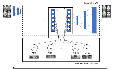
Figure 1: The proposed 2-layer DeepCoder: the input is a face image, and the outputs are the reconstructed face image and AU intensity levels. The top variational convolutional autoencoder (VAE) performs the first level coding ($\boldsymbol{Z}_{0}$) of the facial features, while further encoding ($\boldsymbol{Z}_{1}$) of these features is optimized for AU intensity estimation using ordinal GP variational autoencoder (VO-GPAE).

However, despite the rapid growth in available facial images (videos), there is an overall lack of annotated images (in terms of AUs). This is mainly because it entails a costly and time-consuming labeling effort by trained human annotators. For instance, it may take more than an hour for the expert annotator to code the intensity of AUs in one second of a face video. Even then, the annotations are biased, resulting in a low agreement between the annotators. This is further challenged by a large variability in imaging conditions, facial morphology and dynamics of expressions. Therefore, there is a need for machine learning models that can efficiently and accurately perform the AU coding of target face images.

Recent advances in deep neural networks (DNN), and, in particular, convolutional models (CNNs) [15], have shown great advances towards automating the process of image coding. The effectiveness of these models has been demonstrated on many general vision problems [25, 48, 47]. In the context of facial expression analysis, the majority of existing ’deep’ works consider only baseline tasks such as expression recognition and AU detection [30, 57, 21]. Only a handful of these works attempted AU intensity estimation [15]. This is due to the limited annotated face images of AU intensity (that otherwise could fully be exploited in deep learning), and the difficulty in discerning AU intensities.

Traditionally, the AU intensity estimation has been addressed by non-deep models (SVMs, CRFs, etc.) [54, 17], and using geometric features such as the locations of characteristic facial points, and/or hand-crafted appearance-based features (such as LBPs, Gabors or SIFT). An alternative approach that is being commonly adopted in a variety of computer vision tasks is to automatically extract most informative features from (high-dimensional) input images using the notion of convolutitonal auto-encoders (CAE) [34, 51, 24]. CAE differ from conventional AEs [7] as they are built using convolutional layers with shared weights among neighborhood pixels that preserve the spatial locality. The CAE architectures are typically similar to that of a CNN with additional inverse convolution operation [34]. The key ingredient of CAEs is that they are learned by minimizing the reconstruction loss without the need for image labels, while reducing the effects of noise in the input.

Consider a practical example typically occurring in automated analysis of facial expressions, and, in particular, AU intensity coding: we have access to a large corpora of unlabeled face images, but only a few thousand images are coded in terms of AU intensity. To fully leverage the available data, efficient and highly expressive generative models based on VAE can be used to find a set of underlying features from unlabeled images. Due to the reconstruction cost of VAEs, it is assured that the obtained features represent well the high dimensional face images. Then, highly expressive non-parametric prediction models (e.g., based on GPs [39]) can be applied. This allows them to focus on the main task - in our case, the AU intensity estimation, instead of the computationally expensive feature selection. More importantly, such non-parametric approaches when applied to robust input features are expected to generalize better than their parametric counterparts (e.g., soft-max output layer of DNNs) due to the ability to preserve specific structures in target features – such as subject-specific variation in AU intensity. This is achieved by means of their kernel functions that can focus on data samples in the VAE feature space, effectively doing smoothing over training subjects to make best prediction of AU intensity levels for the test subject.

While the approach described above is a promising avenue for the design of a class of semi-parametric auto-encoding models, independently applying the two models (e.g., VAE for feature extraction, and non-parametric models for AU intensity estimation) is suboptimal as there is no sharing of information (and parameters). To this end, we propose a novel model, named DeepCoder, that leverages the power of parametric and non-parametric VAEs in a unified probabilistic framework. Specifically, DeepCoder is a general framework that builds upon a hierarchy of any number of VAEs, where each coding/decoding part of the intermediate VAEs interacts with the neighboring VAEs during learning, assuring the sharing of information in both directions (bottom-up & top-down). This is achieved through a newly introduced approximate learning of VAEs in DeepCoder. We illustrate this approach by designing an instance of DeepCoder as a two-level semi-parametric VAE (2DC) - the top level being the standard parametric VAE [23], and the bottom level (also used for AU intensity estimation) being a non-parametric Variational Ordinal Gaussian Process AE (VO-GPAE) [12]. We choose these two approaches as their probabilistic formulation allows for tying of their priors over the latent features, in a principled manner. The model is depicted in Fig. (1). We show on two benchmark datasets for AU intensity estimation (DISFA[35] and FERA [50]) that the proposed approach outperforms the state-of-the-art approaches for the AU intensity estimation.

2 Related Work

2.1 Facial Action Unit Intensity Estimation

Estimation of AUs intensity is often posed as a multi-class problem approached using Neural Networks [19], Adaboost [3], SVMs [32] and belief networks [31] classifiers. Yet, these methods are limited to a single output, thus, a separate classifier is learned for each AU - ignoring the AU dependencies. This has been addressed using the multi-output learning approaches. For example, [36] proposed a multi-task learning for AU detection, where a metric with shared properties among multiple AUs was learned. Similarly, [41] proposed a MRF-tree-like model for joint intensity estimation of AUs. [17] proposed Latent-Trees (LTs) for joint AU-intensity estimation that captures higher-order dependencies among the input features and AU intensities. More recently, [54] proposed a multi-output Copula Regression for ordinal estimation of AU intensity. However, these cannot directly handle high-dimensional input face images.

2.2 CNNs for Facial Expression Analysis

CNNs operate directly on the input face images to extract optimal image features. [30] introduced an AU-aware receptive field layer in a deep network, designed to search subsets of the over-complete representation, each of which aims at simulating the best combination of AUs. Its output is then passed through additional layers aimed at the expression classification, showing a large improvement over the traditional hand-crafted features. In [15], a CNN is jointly trained for detection and intensity estimation of AUs. More recently, [57] introduced an intermediate region layer learning region specific weights. These methods are parametric, with the CNN used to extract deep features; yet, the network output remains unstructured. Thus, none of these models exploits CNNs in the context of (ordinal) deep semi-parametric models, as done in DeepCoder. Note also that in DeepCoder we exploit a label-augmented version of VAEs, which can be seen as a variant of CNNs used for classification, but with an additional noise-reduction cost (decoder).

2.3 Autoencoders (AE)

The main idea of AEs is to learn latent representations automatically from inputs, usually in an unsupervised manner [34, 2, 29]. Recenly, variational AEs (VAEs) have gained attention as parametric generative models [14, 23, 22, 45] and their stacked or convolutional variations [26, 27]. Example applications include the reconstruction of noisy and/or partially missing data [52, 53], or feature extraction for classification [7]. Furthermore, AEs based on deep networks have shown their efficacy in many face-related recognition problems [18, 31, 56].

AEs are also closely related to GP Latent Variable Models (GPLVMs) with ”back-constraints” [28, 49, 44]. This mapping facilitates a fast inference mechanism and enforces structure preservation in the latent space. In [10, 8], the authors proposed a variational approximation to the latent space posterior. [16] proposed deep GPs for unsupervised data compression. More recently, [12] introduced a Variational Ordinal GP AE (VO-GPAE), which includes a GP mapping as the decoding model. This allows VO-GPAE to learn the GP encoders/decoders in a joint framework. We extend this formulation of the non-parametric VAE by embedding it into the bottom layer of DeepCoder, while using the (parametric) convolutional AE at the top - achieving an efficient feature extraction.

3 DeepCoder: Methodology

Assume we are given a training dataset $\mathcal{D}=\{\boldsymbol{X},\boldsymbol{Y}\}$, with $N_{\mathcal{D}}$ input images $\boldsymbol{X}=[\boldsymbol{x}_{1},\ldots,\boldsymbol{x}_{i},\ldots,\boldsymbol{x}_{N_{\mathcal{D}}}]^{T}$. The corresponding labels $\boldsymbol{Y}=[\boldsymbol{y}_{1},\ldots,\boldsymbol{y}_{i},\ldots,\boldsymbol{y}_{N_{\mathcal{D}}}]^{T}$ are comprised of multivariate outputs stored in $\boldsymbol{y}_{i}=\{\boldsymbol{y}^{1}_{i},\ldots\boldsymbol{y}^{q}_{i},\ldots\boldsymbol{y}^{Q}_{i}\}$, where $Q$ is the number of AUs, and $\boldsymbol{y}^{q}_{i}$ takes one of $\{1,...,{L^{q}}\}$ intensity levels. Our goal is to predict $\boldsymbol{y}_{*}$ and reconstruct $\boldsymbol{x}_{*}^{^{\prime}}$, given a new test input image $\boldsymbol{x}_{*}$. To learn the highly non-linear mappings $\boldsymbol{X}\to\boldsymbol{Y}$, we perform encoding and decoding of input features $\boldsymbol{X}$ via multiple layers of VAEs. These layers are encoded by the latent variables $\boldsymbol{Z}=\{\boldsymbol{Z}_{i}\},\;i=0,\dots,N-1$, where the dimension of $\boldsymbol{Z}_{i}$ can vary for each $i$, and $N$ is the number of layers. For simplicity, we first assume a single VAE layer with latent variables $\boldsymbol{Z}_{0}$. This leads to the following marginal log-likelihood and its corresponding variational lower bound:

$$\log p(\boldsymbol{X},\boldsymbol{Y})= \log\int p(\boldsymbol{X}|\boldsymbol{Z}_{0})p(\boldsymbol{y}|\boldsymbol{Z}_{0})p(\boldsymbol{Z}_{0})d\boldsymbol{Z}_{0}$$ (1)

$$\begin{split}\geq\;&\mathbb{E}_{q(\boldsymbol{Z}_{0}|\boldsymbol{X})}\big{[}\log p(\boldsymbol{X}|\boldsymbol{Z_{0}})\big{]}\\ &+\mathbb{E}_{q(\boldsymbol{Z}_{0}|\boldsymbol{X})}\big{[}\log p(\boldsymbol{Y}|\boldsymbol{Z}_{0})\big{]}\\ &-D_{KL}(q(\boldsymbol{Z}_{0}|\boldsymbol{X})||p(\boldsymbol{Z_{0}}))\\ \end{split}$$ (2)

In Eq. (1), the first two terms are the reconstruction loss over the input features and output labels, respectively, under the estimated posterior. The second term is the Kullback-Leibler (KL) divergence which measures the difference between the approximate and true posterior. We obtain the latter by exploiting the conditional independence $\boldsymbol{X}\perp\!\!\!\perp\boldsymbol{y}|\boldsymbol{Z}_{0}$ (see [12] for details). To account for more complex dependencies between $(\boldsymbol{X},\boldsymbol{Y})$, we generalize Eq. (LABEL:lowerbound) by expanding $p(\boldsymbol{Z}_{0})$ as a stack of $N$ VAE layers (see Fig. (2))

$$\begin{split}&\underbrace{\textstyle\int p(\boldsymbol{Z}_{0}|\boldsymbol{Z_{1}})\ldots\underbrace{\textstyle\int p(\boldsymbol{Z}_{N-1}|\boldsymbol{Z_{N}})p(\boldsymbol{Z_{N}})d\boldsymbol{Z}_{N}}_{\begin{subarray}{c}\tilde{p}(\boldsymbol{Z}_{n-1})\\ \vdots\end{subarray}}\ldots d\boldsymbol{Z}_{1}}_{\tilde{p}(Z_{0})}\end{split}$$ (3)

Figure 2: The general formulation of DeepCoder as a stack of $N$ VAEs, modeling the input-output pairs: ($\boldsymbol{X}$,$\boldsymbol{Y}$). The conditionals $(\boldsymbol{Z}_{0}|\boldsymbol{X}),\ldots(\boldsymbol{Y}|\boldsymbol{Z}_{N})$ from left to right in DeepCoder perform the coding part, while from right to left perform the decoding part via $(\boldsymbol{Z}_{N-1}|\boldsymbol{Z}_{N}),\ldots(\boldsymbol{X}|\boldsymbol{Z}_{0})$. Note that for N=2, we obtain the proposed 2-layer DeepCoder, modeled using VC-AE and VO-GPAE, respectively.

This approach has high modeling power; however, it comes with the cost of having to simultaneously learn multiple (deep) layers of latent variables $\boldsymbol{Z}$. While this is computationally tractable for a single layer ($\boldsymbol{Z}_{0}$), in the case of more layers, we need to resort to approximate methods. To this end, we propose an optimization approach that sequentially performs a chain-like propagation of uncertainty of each coder. Specifically, we solve for the posteriors of each coder ’locally’ and use the learned posteriors to define the (approximate) prior $p(\boldsymbol{Z})$, needed to compute the KL divergence of each subsequent coder in the sequence from ’bottom-up’ (a practical example of this is described in Alg. (1)). For the $(N-1)$-th VAE, instead of using a flat Gauss prior $p(\boldsymbol{Z}_{N-1})$, we approximate it using the posterior of the $N$-th decoder learned as:

$$\begin{split}\log\tilde{p}(\boldsymbol{Z}_{n-1})\geq&\mathbb{E}_{q(\boldsymbol{Z}_{N}|\boldsymbol{Z}_{N-1})}\big{[}\log p(\boldsymbol{Z}_{N-1}|\boldsymbol{Z}_{N})\big{]}\\ &-D_{KL}(q(\boldsymbol{Z}_{N}|\boldsymbol{Z}_{N-1})||\tilde{p}(\boldsymbol{Z_{N}}))\end{split}$$ (4)

Note the main benefit of the proposed: instead of assuming a flat prior over the latent variables, as typically done in existing VAE [23], we define the priors on $\boldsymbol{Z}$ that are informed of the uncertainty of each coder ’below’ in the deep structure, while also retaining the information about the decoding error of all subsequent coders. Thus, by exploiting the conditional independence of $\boldsymbol{Z}$ at each level of DeepCoder, we seamlessly ’encode’ complex relationships between $\boldsymbol{X}$ and $\boldsymbol{Y}$. From the regularization perspective, we constrain the parameters via the KL terms (based on priors $\tilde{p}(\boldsymbol{Z})$) at each level of coding/decoding in DeepCoder. Fig. (2) illustrates the main idea for the general case. Using this framework, we generate an instance of DeepCoder as a two-layer semi-parametric coder: the top coder takes the parametric form (Convolutional VAE) and the bottom the non-parametric form (VAE based on GPs). We choose these two because their probabilistic formulation allows us to combine them in a Bayesian framework. Also, instead of using directly CNNs in the first layer, we opt for using VAEs due to their de-noising of input features (although we augment the subspace learning using target labels as in CNNs).

3.1 Variational Convolutional AEs (VC-AE)

In the top layer, we use the VC-AE to map the inputs $\boldsymbol{X}$ onto the latent space $\boldsymbol{Z}_{0}$. A decoder network is then used to map these latent space points back to the original input data. Formally, the parameters of VC-AE are learned by maximizing the objective:

$$\begin{split}\mathcal{L}_{VC-AE}(W_{d},\mu,\sigma)&=\mathcal{L}_{kl,\boldsymbol{X}}+\mathcal{L}_{r,\boldsymbol{X}}\\ \mathcal{L}_{kl,\boldsymbol{X}}&=-D_{KL}(q_{\mu,\sigma}(\boldsymbol{Z}_{0}|\boldsymbol{X})||p(\boldsymbol{Z}_{0}))\\ \mathcal{L}_{r,\boldsymbol{X}}&=\mathbb{E}_{q(\boldsymbol{Z}_{0}|\boldsymbol{X})}\big{[}\log p(\boldsymbol{X}|\boldsymbol{Z}_{0})\big{]}\end{split}$$ (5)

where the KL divergence ($\mathcal{L}_{kl,\boldsymbol{X}}$) and reconstruction term ($\mathcal{L}_{r,\boldsymbol{X}}$), form the variational lower bound typically optimized in VC-AEs. The conditionals are parametrized as:

$$\boldsymbol{X}|\boldsymbol{Z}_{0} =f_{\boldsymbol{Z}_{0}\to\boldsymbol{X}}(\cdot;\theta_{\boldsymbol{Z}_{0}\to\boldsymbol{X}}),$$ (6)

$$\boldsymbol{Z}_{0}|\boldsymbol{X} =f_{\boldsymbol{X}\to\boldsymbol{Z}_{0}}(\cdot;\theta_{\boldsymbol{X}\to\boldsymbol{Z}_{0}}).$$ (7)

Their functional forms are given by the VC encoder ($\boldsymbol{Z}_{0}|\boldsymbol{X}$) and decoder ($\boldsymbol{X}|\boldsymbol{Z}_{0})$. For the convolutional coder part ($\theta_{\boldsymbol{Z}_{0}\to\boldsymbol{X}}$), we used 5 convolutional layers containing 128, 64, 32, 16 and 8 filters. The filter size was set to $5\times 5$ pixel followed by ReLu (Rectified Linear Unit) activation functions [23]. We also used $2\times 2$ max pooling layers after each convolutinonal layer. The compressed representations are $15\times 20\times 16$ pixels and are passed to two fully connected layers, which return $2000$ features each, with the latent space variational posterior $q(\boldsymbol{Z}_{0}|\boldsymbol{X})\sim\mathcal{N}(\mu,\sigma^{2})$. For deconvolution ($\theta_{\boldsymbol{X}\to\boldsymbol{Z}_{0}}$), we used up-scaling instead of max-pooling and deployed the inverse encoder architecture. For this, we exploited the re-parameterization trick [23]. We sample points $z$ at random from the distribution of latent variables $\boldsymbol{Z}_{0}$, in order to generate the data. Finally, the decoder network maps $z$ back to the original input.

3.2 Variational Ordinal GP AEs (VO-GPAE)

We employ the VO-GPAE [12] approach to model the second VAE in DeepCoder: $\boldsymbol{Z}_{0}\in\mathbb{R}^{N_{D}\times N_{D_{0}}}$ being the input and $\boldsymbol{Z}_{1}$ the corresponding latent variables. Similar to VC-AEs (Sec. (3.1)), the objective of this layer becomes:

$$\begin{split}\mathcal{L}_{VO-GPAE}(W_{o},\theta_{GP},V)&=\mathcal{L}_{kl,\boldsymbol{Z}_{0}}+\mathcal{L}_{r,\boldsymbol{Z}_{0}}+\mathcal{L}_{o,\boldsymbol{Z}_{0}}\\ \mathcal{L}_{kl,\boldsymbol{Z}_{0}}&=-D_{KL}(q(\boldsymbol{Z}_{1}|\boldsymbol{Z}_{0})||p(\boldsymbol{Z}_{1}))\\ \mathcal{L}_{r,\boldsymbol{Z}_{0}}&=\sum_{d=0}^{D_{0}}\mathbb{E}_{q(\boldsymbol{Z}_{1}|\boldsymbol{Z}_{0})}\big{[}\log p(\boldsymbol{z}_{0}^{d}|\boldsymbol{Z}_{1})\big{]}\\ \mathcal{L}_{o,\boldsymbol{Z}_{0}}&=\mathbb{E}_{q(\boldsymbol{Z}_{1}|\boldsymbol{Z}_{0})}[\log p(\boldsymbol{Y}|\boldsymbol{Z_{1}},W_{o})],\end{split}$$ (8)

where

$$\boldsymbol{Z}_{0}|\boldsymbol{Z}_{1} =f_{\boldsymbol{Z}_{1}\to\boldsymbol{Z}_{0}}(\cdot;\theta_{\boldsymbol{Z}_{1}\to\boldsymbol{Z}_{0}}),$$ (9)

$$\boldsymbol{Z}_{1}|\boldsymbol{Z}_{0} =f_{\boldsymbol{Z}_{0}\to\boldsymbol{Z}_{1}}(\cdot;\theta_{\boldsymbol{Z}_{0}\to\boldsymbol{Z}_{1}}),$$ (10)

$$\boldsymbol{Y}|\boldsymbol{Z}_{1} =f_{\boldsymbol{Z}_{1}\to\boldsymbol{Y}}(\cdot;W_{o}).$$ (11)

Here, $f_{\boldsymbol{Z}_{1}\to\boldsymbol{Z}_{0}}$ and $f_{\boldsymbol{Z}_{0}\to\boldsymbol{Z}_{1}}$ are the encoding and decoding mappings with GP priors, $\theta_{\boldsymbol{Z}_{1}\to\boldsymbol{Z}_{0}}$ and $\theta_{\boldsymbol{Z}_{0}\to\boldsymbol{Z}_{1}}$ are the corresponding kernel parameters, and $f_{\boldsymbol{Z}_{1}\to\boldsymbol{Y}}$ is the classification function. We place GP priors on both mappings, resulting in:

$$p(\boldsymbol{Z_{0}}|\boldsymbol{Z_{1}})=\mathcal{N}(\boldsymbol{0},\boldsymbol{K}_{\boldsymbol{Z}_{1}\to\boldsymbol{Z}_{0}}+\sigma_{v}^{2}\boldsymbol{I}),$$ (12)

$$p(\boldsymbol{Z_{1}}|\boldsymbol{Z_{0}})=\mathcal{N}(\boldsymbol{0},\boldsymbol{K}_{\boldsymbol{Z}_{0}\to\boldsymbol{Z}_{1}}+\sigma_{r}^{2}\boldsymbol{I}),$$ (13)

$$p(\boldsymbol{Z}_{0})=\int\prod_{d=1}^{D_{0}}p(\boldsymbol{z}_{0}^{d}|\boldsymbol{Z}_{1})p(\boldsymbol{Z}_{1})d\boldsymbol{Z}_{1},$$ (14)

where $D_{o}$ is the dimension of $\boldsymbol{Z}_{0}$. Since computing its marginal likelihood is intractable (due to the non-linear coupling of the GP kernels), we resort to approximations. To this end, the approximate variational distribution $q(\boldsymbol{Z_{1}}|\boldsymbol{Z_{0}})$ is used to recover a Bayesian non-parametric solution for both the GP encoder & decoder, and is defined as:

$$q(\boldsymbol{Z}_{1}|\boldsymbol{Z}_{0})=\prod\nolimits_{i}\mathcal{N}(\hat{\boldsymbol{m}}_{i},\boldsymbol{S}_{i}+\hat{\sigma}_{i}^{2}I),$$ (15)

where $\boldsymbol{M}=\{\boldsymbol{m}_{i}\},\;i=1,...,N$ and $\boldsymbol{S}=\{\boldsymbol{S}_{i}\},\;i=1,...,N$ are variational parameters, and $\hat{\boldsymbol{m}}_{i}=\boldsymbol{m}_{i}-\left[\boldsymbol{K}_{\boldsymbol{Z}_{1}\to\boldsymbol{Z}_{0}}^{-1}\boldsymbol{M}\right]_{i}/\left[\boldsymbol{K}_{\boldsymbol{Z}_{1}\to\boldsymbol{Z}_{0}}^{-1}\right]_{ii}$ and $\hat{\sigma}_{i}^{2}=1/\left[\boldsymbol{K}_{\boldsymbol{Z}_{1}\to\boldsymbol{Z}_{0}}^{-1}\right]_{ii}$ is the leave-one-out solution of GP [39].

We further constrain the latent variable $\boldsymbol{Z_{1}}$ by imposing the ordinal structure on the output labels $\boldsymbol{Y}$ as:

$$p(\boldsymbol{Y}|\boldsymbol{Z_{1}}) =\prod_{i,c}\mathbbm{I}{(\boldsymbol{y}_{i}=c)}p(\boldsymbol{y}_{i}|\boldsymbol{z}_{1i})\quad,$$ (16)

$$p(\boldsymbol{y}_{i}=s|\boldsymbol{z}_{1i}) =\begin{cases}1\quad$if $f_{\boldsymbol{Z}_{1}\to\boldsymbol{Y}}(\boldsymbol{z}_{1i})\in(\gamma_{c,s-1},\gamma_{c,s}]\\ 0\quad$otherwise$,\end{cases},$$ (17)

$$f_{\boldsymbol{Z}_{1}\to\boldsymbol{Y}}(\boldsymbol{z_{1i}}) =w_{o}^{T}\boldsymbol{z}_{1i}+\epsilon,\;\epsilon\sim\mathcal{N}(0,\sigma^{2}_{o}),$$ (18)

where $\mathbbm{I}{(\mathord{\cdot})}$ is the indicator function that returns 1 (0) if the argument is true (false) and $i=1,\dots,N$ indexes the training data. $\gamma_{c,0}=-\infty\leq\cdots\leq\gamma_{c,S}=+\infty$ are the thresholds or cut-off points that partition the real line into $s=1,\dots,S$ contiguous intervals. We arrive at the ordinal log-likelihood (see [5] for details):

$$\begin{split}\mathbb{E}_{q(\boldsymbol{Z}_{1}|\boldsymbol{Z}_{0})}(\log p(\boldsymbol{Y}|\boldsymbol{Z}_{1},\boldsymbol{W}_{o}))=\sum_{i,c}\mathbb{I}(y_{ic}=s)\log\\ \biggl{(}\Phi\left(\frac{\gamma_{c,s}-\boldsymbol{w}_{o}^{T}\boldsymbol{z}_{1i}}{\sigma_{o}}\right)-\Phi\left(\frac{\gamma_{c,s-1}-\boldsymbol{w}_{o}^{T}\boldsymbol{z}_{1i}}{\sigma_{o}}\right)\biggr{)}\end{split}$$ (19)

where $\Phi(\cdot)$ is the Gaussian cumulative density function.

The random process of recovering the latent variables has two distinctive stages: (a) the latent variables $\boldsymbol{Z}_{1}$ are generated from some general prior distribution $p(\boldsymbol{Z_{1}})=\mathcal{N}(\boldsymbol{0},\boldsymbol{I})$, and further projected to the labels’ ordinal plane via $p(\boldsymbol{Y}|\boldsymbol{Z_{1}})$; (b) the input $\boldsymbol{Z}_{1}$ is generated from the conditional distribution $p(\boldsymbol{Z}_{1}|\boldsymbol{Z}_{0})$. The model parameters are: $\theta_{GP}=\{\theta_{\boldsymbol{Z}_{1}\to\boldsymbol{Z}_{0}},\;\theta_{\boldsymbol{Z}_{0}\to\boldsymbol{Z}_{1}}\}$, $W_{o}=\{w_{o},\;\sigma_{o}\}$, and $V=\{M,S\}$ are variational parameters.

4 Learning and Inference

Learning of DeepCoder consists of maximizing the joint lower bound (Sec. (4.3)) w.r.t the VC-AEs parameters ($W_{d}$, $\mu$, $\sigma$) and the VO-GPAE (hyper-) parameters ($V$, $\theta_{GP}$,$W_{o}$). For the GP-encoder/decoder kernel, we use the radial basis function (RBF) with automatic relevance determination (ARD), which can effectively estimate the dimensionality of the latent space [9]. For both VC-AE and VO-GPAE, we utilize a joint optimization scheme using stochastic backpropagation [40], with the re-parameterization trick [23]. Before we detail the steps of our learning algorithm, we first describe the proposed iterative balanced batch learning (Sec. (4.1)) and the warming criterion to efficiently learn the latent features (Sec. (4.2)). These strategies turn out to be critical in avoiding overfitting and achieving significant learning speed-ups.

4.1 Iterative Balanced Batch Learning

Minimizing the model objective using all training data can easily lead to a local minimum, and, thus, poor performance. This is due to the inherent hierarchical structure of the model (VAE layers), and highly imbalanced AU intensity labels. We introduce an iterative balanced batch learning approach to deal with the data imbalance. The main idea is to update each set of parameters with batches that are balanced with respect to subjects in the dataset (number of example images of each subject) and AU intensity levels. This ensures that the network used for facial feature extraction is not biased towards a specific subject/AU level. We use Stochastic Gradient Descent (SGD) with a batch size of 32, learning rate of 0.01 and momentum of 0.9.

4.2 Warming Strategy

The lower bound in Eq. (5&8) consists of three terms. Each model that encodes a latent variable $\boldsymbol{Z}_{i}$ will have a non-zero KL term and a relatively small cross-entropy term. Practically, implementations of such AEs will struggle to learn this behavior. As pointed out in [46, 4, 38], training these models will lead to consistently setting the approximate distribution $q(\boldsymbol{Z}_{i}|\boldsymbol{Z}_{i-1})$ equal to the prior $p(\boldsymbol{Z}_{i})$, and thus bringing the KL divergence to zero. This can be of advantage and seen as ARD, but also be a challenge in training for the latent space to learn a useful (and discriminative) representation. To avoid this, we propose different warm-up strategies for training VAEs in DeepCoder. Specifically, instead of directly maximizing the lower bound of the VC-AE (Eq.(5)), we augment the learning by including the expectation of the predicted labels ($\mathcal{L}_{p}$) for intensity classification of AUs, steering the parameters towards more discriminative latent representations. Formally, this is attained by using the weighted objective given by:

$$\mathcal{L}_{VC-AE}=\alpha\mathcal{L}_{kl,\boldsymbol{X}}+\mathcal{L}_{r,\boldsymbol{X}}+(1-\alpha)\mathcal{L}_{p,\boldsymbol{X}},$$ (20)

where

$$\mathcal{L}_{p,\boldsymbol{X}} =\mathbb{E}_{q(\boldsymbol{Z}_{0}|\boldsymbol{X})}\big{[}\log(p(\boldsymbol{Y}|\boldsymbol{Z}_{0},W_{d}))\big{]},$$ (21)

$$\boldsymbol{Y}|\boldsymbol{Z}_{0} =f_{\boldsymbol{Z}_{0}\to\boldsymbol{Y}}(\cdot;W_{c}).$$ (22)

Here, $(\boldsymbol{Y}|\boldsymbol{Z_{0}})$ can be modeled using any classifier $W_{c}$ (we used logistic regression). Note that initially ($\alpha=0$) we focus on finding a discriminative subspace at the first layer of DeepCoder. With the increasing number of iterations, the KL divergence term overtakes the classification loss, assuring the smoothness of the subspace $\boldsymbol{Z}_{0}$. We then construct a lower bound for VO-GPAE with a warming term as:

$$\mathcal{L}_{VO-GPAE} =\beta\mathcal{L}_{kl,\boldsymbol{Z}_{0}}+\mathcal{L}_{r,\boldsymbol{Z}_{0}}+\mathcal{L}_{o,\boldsymbol{Z}_{0}}.$$ (23)

Both $\alpha$ and $\beta$ are linearly increased from 0 to 1 during the first $N_{t}$ epochs of training. Note that in the beginning, we include the classification loss in the first layer - which acts as a regularizer. However, it slowly diminishes as we obtain more stable estimates of the variational distributions at each layer, since toward reaching the $N_{t}$-th epoch, the VO-GPAE classifier stabilizes and $\boldsymbol{Z}_{0}$ need no more be class-regularized. We found that this approach works very well in practice, as shown in Sec. (5).

4.3 Joint Learning

In the 2-layer DeepCoder, we optimize the lower bound:

$$\mathcal{L}_{DC}=\mathcal{L}_{VC-AE}+\mathcal{L}_{VO-GPAE}.$$ (24)

The main bottleneck of the second AE is that it cannot use all training data as the computation of covariance function in VO-GPAE would be prohibitively expensive. Because of this, we propose a ’leave-subset-out’ strategy, where we learn the target AEs in an iterative manner. Specifically, we split the training dataset $\boldsymbol{X}$ in two non-overlapping subsets, $X_{R}$ and $X_{L}$, $X_{R}>>X_{L}$. $X_{R}$ is used for training VC-AE, while $X_{L}$ is used for training VO-GPAE. First, VC-AE is initialized using $X_{R}$ by minimizing Eq. (5) for 5 epochs, followed by the two-step iterative training algorithm. In the first step, we find the latent projections using $X_{L}$, i.e., $\boldsymbol{Z}_{0,L}$ by VC-AE and learned parameter $W_{d}$, $\mu_{R}$ and $\sigma_{R}$ from $X_{R}$. $\boldsymbol{Z}_{0,L}$ are then used to train VO-GPAE for one epoch, minimizing Eq. (8). In the second step, we reconstruct $X_{R}$ as $\boldsymbol{Z}_{0,R}$, and also compute the posteriors $\tilde{p}(\boldsymbol{Z}_{0,R})$, which are then fed into the VC-AE to update its parameters by minimizing Eq. (5) in one epoch. These two steps are repeated until convergence of the joint lower bound $\mathcal{L}_{2DC}$. In this way, we constantly update the prior on $\boldsymbol{Z}_{0}$, which propagates the information from the bottom VO-GPAE, effectively tying the parameters of the two AEs.

Algorithm 1 DeepCoder: Learning and Inference

Learning: Input $\mathcal{D}_{tr}=(\boldsymbol{X},\boldsymbol{y})$

Split $\boldsymbol{X}\in\boldsymbol{X}_{R}\cup\boldsymbol{X}_{L}$, $\boldsymbol{X}_{R}>>\boldsymbol{X}_{L}$, and $\boldsymbol{X}_{R}\cap\boldsymbol{X}_{L}=\emptyset$.

repeat

    if init run, $p(\boldsymbol{Z}_{0,R})\sim\mathcal{N}(0,1)$

    else $\tilde{p}(\boldsymbol{Z}_{0,R})=p(\boldsymbol{Z}_{0,R}|\boldsymbol{Z}_{1,L})$ end

    Step 1: for 1 epoch, optimize $\mathcal{L}_{VC-AE}$ given $\boldsymbol{X}_{R}$,

          $\boldsymbol{Z}_{0,R}=f_{\boldsymbol{X}\to\boldsymbol{Z_{0}}}(X_{R})$   and   $\boldsymbol{Z}_{0,L}=f_{\boldsymbol{X}\to\boldsymbol{Z_{0}}}(X_{L})$

    Step 2: for 1 epoch, optimize $\mathcal{L}_{VO-GPAE}$ given $\boldsymbol{Z}_{0,L}$,

          $\boldsymbol{Z}_{0,R}=f_{\boldsymbol{Z_{1}}\to\boldsymbol{Z_{0}}}(f_{\boldsymbol{Z}_{0}\to\boldsymbol{Z}_{1}}(Z_{0,R}))$

until convergence of $\mathcal{L}_{2DC}$

Output: $W_{d},\mu_{R},\sigma_{R},W_{o},\theta_{GP},V_{L}$

Inference: Input $\mathcal{D}_{te}=(\boldsymbol{X}_{*})$

Step 1: $\boldsymbol{Z}_{1,*}=f_{\boldsymbol{Z}_{0}\to\boldsymbol{Z}_{1}}(f_{\boldsymbol{X}\to\boldsymbol{Z}_{0}}(\boldsymbol{X}_{*},W_{d}))$

Step 2: $\boldsymbol{y}_{*}=f_{\boldsymbol{Z_{1}}\to\boldsymbol{Y}}(\boldsymbol{Z}_{1,*},W_{o})$

                  $\boldsymbol{X}^{\prime}_{*}=f_{\boldsymbol{Z}_{0}\to\boldsymbol{X}}(f_{\boldsymbol{Z}_{1}\to\boldsymbol{Z}_{0}}(\boldsymbol{Z}_{1,*}),W_{d})$

Output: $\boldsymbol{X}^{\prime}_{*},\;\boldsymbol{y_{*}}$

Table 1: Performance of different models for AU intensity estimation on the DISFA and FERA2015 database. DC- and CNN-based models were trained using raw images as input. The results for the models highlighted with $\dagger$ were taken from [12] (the model trained with LBP+landmark features). The model highlighted with $\star$ was trained with the deep features, extracted from the last layer of the best performing CNN [15], and, thus, is directly comparable to the proposed 2DC.

Dataset:		DISFA													FERA2015
AU:		1	2	4	5	6	9	12	15	17	20	25	26	Avg.	6	10	12	14	17	Avg.
ICC	2DC	.70	.55	.69	.05	.59	.57	.88	.32	.10	.08	.90	.50	.50	.76	.71	.85	.45	.53	.66
	DCp	.52	.49	.48	.18	.59	.39	.74	.15	.26	.08	.80	.44	.43	.74	.72	.84	.33	.52	.63
	CNN [15]	.58	.52	.55	.20	.59	.42	.78	.08	.25	.04	.84	.54	.44	.76	.70	.85	.36	.49	.63
	OR-CNN [37]	.33	.31	.32	.16	.32	.28	.71	.33	.44	.27	.51	.36	.36	.71	.63	.87	.41	.31	.58
	CCNN-IT [55]	.18	.15	.61	.07	.65	.55	.82	.44	.37	.28	.77	.54	.45	.75	.69	.86	.40	.45	.63
	VGG16 [43]	.46	.44	.44	.06	.44	.34	.59	.01	.11	.03	.71	.42	.32	.63	.61	.73	.25	.31	.51
	VO-GPAE [12]⋆	.18	.00	.27	.15	.57	.34	.80	.01	.00	.02	.88	.55	.31	.72	.66	.78	.43	.56	.63
	VO-GPAE [12]†	.48	.47	.62	.19	.50	.42	.80	.19	.36	.15	.84	.53	.46	.75	.66	.88	.47	.49	.65
	VAE-DGP [8]⋆	.37	.32	.43	.17	.45	.52	.76	.04	.21	.08	.80	.51	.39	.70	.68	.78	.43	.31	.58
	GP [39]⋆	.26	.11	.32	.12	.45	.32	.31	.02	.18	.06	.85	.42	.28	.61	.57	.71	.32	.35	.51
	SOR [1]⋆	.15	.13	.34	.03	.48	.22	.78	.00	.10	.06	.79	.42	.29	.61	.57	.77	.29	.27	.50
	MLR⋆	.45	.39	.30	.11	.52	.26	.72	.09	.00	.01	.82	.39	.29	.74	.67	.81	.42	.25	.57
MSE	2DC	.32	.39	.53	.26	.43	.30	.25	.27	.61	.18	.37	.55	.37	.75	1.02	.66	1.44	.88	.95
	DCp	.35	.44	.90	.03	.36	.36	.37	.26	.30	.19	.71	.57	.40	.85	1.03	.75	1.80	0.81	1.05
	CNN [15]	.34	.39	.81	.05	.37	.38	.34	.27	.31	.24	.63	.49	.38	.80	1.06	.66	1.57	.96	1.01
	OR-CNN [37]	.41	.44	.91	.12	.42	.33	.31	.42	.35	.27	.71	.51	.43	.88	1.12	.68	1.52	.93	1.02
	CCNN-IT [55]	.76	.40	.74	.07	.54	.41	.33	.14	.33	.20	.66	.41	.41	1.23	1.69	.98	2.72	1.17	1.57
	VGG16 [43]	.41	.54	1.14	.07	.39	.47	.40	.29	.53	.19	.64	.51	.39	.93	1.04	.91	1.51	1.10	1.10
	VO-GPAE [12]⋆	1.18	.77	1.14	.11	.22	.53	.16	.18	.99	.81	.21	.46	.56	0.9	.98	.67	1.81	1.31	1.11
	VO-GPAE [12]†	.51	.32	1.13	.08	.56	.31	.47	.20	.28	.16	.49	.44	.41	.82	1.28	.70	1.43	.77	1.00
	VAE-DGP [8]⋆	1.02	1.13	.92	.10	.67	.19	.33	.46	.58	.19	.69	.65	.57	.93	1.15	.80	1.66	1.14	1.13
	GP [39]⋆	.49	.60	1.06	.08	.38	.30	.26	.25	.30	.19	.61	.69	.63	1.07	1.27	1.03	1.52	0.94	1.17
	SOR [1]⋆	1.35	.57	1.43	.09	.46	1.48	.40	.25	.62	.49	1.27	.93	.78	1.59	1.71	1.06	2.90	2.24	1.90
	MLR⋆	.42	.49	1.04	.05	.40	.33	.45	.23	.24	.13	.62	.55	.41	.84	1.06	.72	1.35	1.04	1.00

Inference in the proposed 2DC: the test data $\boldsymbol{X}_{*}$ is first projected to the latent space $\boldsymbol{Z}_{0}$ via the VC-AE, and then further passed through the VO-GPAE via $\boldsymbol{Z}_{1}$. The obtained latent positions are then used for ordinal classification of target AU intensities. The decoding starts with the reconstruction of the latent points in $\boldsymbol{Z}_{0}$, followed by the reconstruction of $\boldsymbol{X}_{*}$. These steps are summarized in Alg. (1).

5 Experiments

Datasets. We evaluate the proposed DeepCoder on two benchmark datasets for AU intensity estimation: DISFA [35] and FERA2015 challenge data [50]. Both contain per frame AU intensity annotations on a 6-point ordinal scale (DISFA 12, FERA2015 6 AUs). Also, we performed subject-independent validation: DISFA (3 folds: 18 train/9 test subjects), and FERA2015 (2 fold: 21 train / 20 test).

Pre-Processing. For the CNN-based models, we used the dlib face detector [20] to extract the face location from images in each dataset. We then registered the 49 facial points to a reference frame (average points in each dataset) using a similarity transform and cropped a bounding box of $240\times 160$ pixel size. These were then normalized using per-image histogram-equalization, which increases the robustness against illumination changes. For models in which it is not feasible to process high dimensional features from raw images, we extracted the 2000-D features ($\boldsymbol{Z}_{0}$) from the CNN - in our experiments, this size was found optimal for the competing methods. During evaluation, we used the negative log-predictive density (NLPD) for the reconstruction error, and for classification the mean squared error (MSE), the classifier’s consistency of the relative order of the intensity levels, and intra-class correlation (ICC(3,1)) [42] - agreement between annotators.

Models. As a baseline, we use the multivariate linear regression (MLR) for joint estimation of AU intensities and the standard ordinal regression (SOR) [1] serves as the second baseline. The CNN [15] model is a standard 2-layer CNN for multi-output classification (we used the same setting as in [15]). The OR-CNN [37] is an ordinal CNN that was originally introduced for the task of age estimation; we applied it to our task. VGG16 [43] is a widely used NN for object detection. To adapt it for our task, we used the pre-trained model and fine-tuned the last 3 layers. As a baseline for the GP-based models, we use the standard GP [39] with a shared covariance function among outputs. We also compare the proposed to VO-GPAE [12], the state-of-the-art GP model for variational ordinal regression. Here, we evaluated the model on two sets of features: LBPs with facial landmarks, and deep features, extracted using the CNN (our first coder). We evaluate the proposed model in two settings: DC_p is the fully parametric DeepCoder (DC_p), where we simply apply a stack of two VC-AEs with a 50D latent space ($\boldsymbol{Z}_{1}$) and 2000D ($\boldsymbol{Z}_{0}$) features- as also set in our semi-parametric 2DC model, with VO-GPAE at the bottom layer. For the iterative 2DC learning algorithm, we split the dataset according to the algorithm in two subsets $N_{L}$ and $N_{R}$. Due to the computational complexity of GPs ($\mathbb{O}(N^{3})$), we chose a rather small subset of $N_{L}=5000$ to train the VO-GPAE, while using the rest of data set for our convolutional auto-encoder VC-AE ($N_{R}=71223$ for FERA2015 and $N_{R}=87209$ for DISFA). For subset $N_{L}$, we also chose a subject balanced subset, i.e. every subject is equally represented in the number of frames. We used the pre-processed raw images as input to the proposed DeepCoder and CNN based models. As the GP-based models and the other baselines are not directly applicable to high dimensional image data, we trained on the LBP+landmark features and/or deep features, extracted from the last layer of the best performing CNN [15] model. For the sake of comparisons, we also include the results from the recently published deep structured learning model with the database augmentation - CCNN-IT [55] (we show the reported results).

6 Results

Quantitative Results. Table (1) shows the comparative results. On average, the CNN based models largely outperform the GPs in both measures across most of the AUs. This is because CNNs are capable to jointly learn the embedded space and classifier from raw images, while GPs are trained on hand-crafted features, which turn out to be less discriminative for the task. This can be particularly observed from AU17 in both datasets. Also, both the relative shallow CNN [15] and the DC_p model achieve an ICC of 44%/43% on DISFA and 63% on FERA2015, which is highest performance using current deep models. By comparing the predictions of these two models, we see that the performance of the fully parametric DC_p does not increase by blindly stacking VC-AEs on top of each other. The same applies to the basic CNNs models. Furthermore, both models are outperformed by the proposed semi-parametric 2DC. This is mainly because GPs are known to provide a better classifier (non-parametric, hence they are more flexible in modeling complex distributions). This can be seen from Fig. ( 3), where the samples on the latent space ${\bf Z}_{1}$ are clustered into different subjects. Note that this subject clustering in the latent space has been done in an unsupervised manner by GPs (i.e., no subject id was provided). The bottom VO-GPAE layer benefits from the robust features coming from the top VC-AE, and the jointly learned ordinal classifier using the proposed iterative algorithm (Alg. (1)).

The standard VGG16 [43] network does not achieve competitive results with the proposed model, most likely because it does not account for ordinal intensity levels and does not perform simultaneous learning of latent features. The OR-CNN [37] model, which has the same architecture as CNN [15] but with the ordinal classifier, learns one binary classifier for each intensity level of each AU, resulting in a large number of parameters, easily prone to overfitting. Overall, from average results on both datasets, we clearly see the benefits of the joint learning in the proposed DeepCoder (2DC). Finally, note that the proposed DeepCoder outperforms the state-of-the-art approach (CCNN-IT [55]), which takes advantage of CNNs and data augmentation based on multiple face datasets. Again, we attribute this to the lack of non-parametric feature learning and ordinal classifier in the latter.

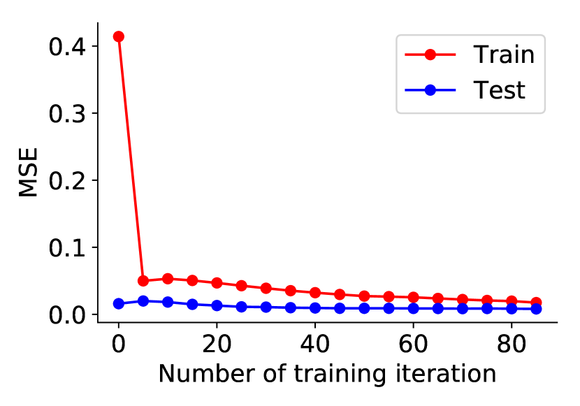
(a) MSE

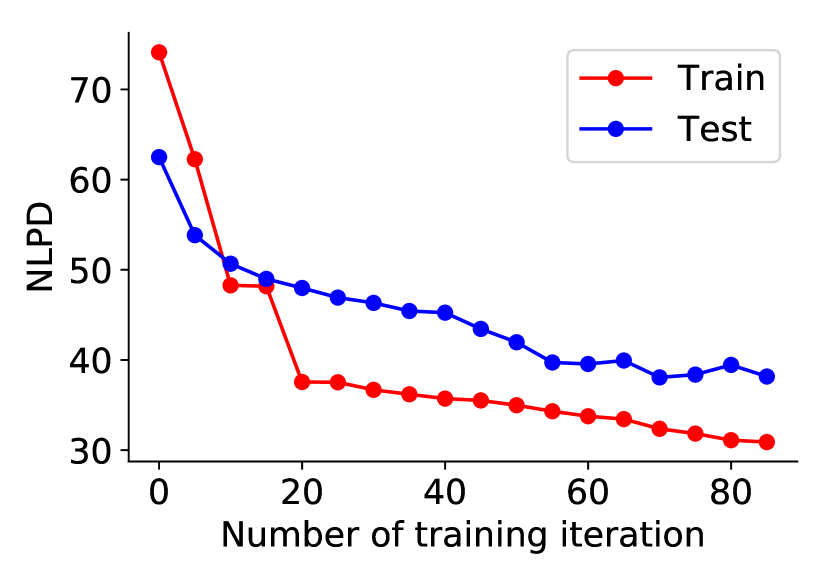
(b) NLPD

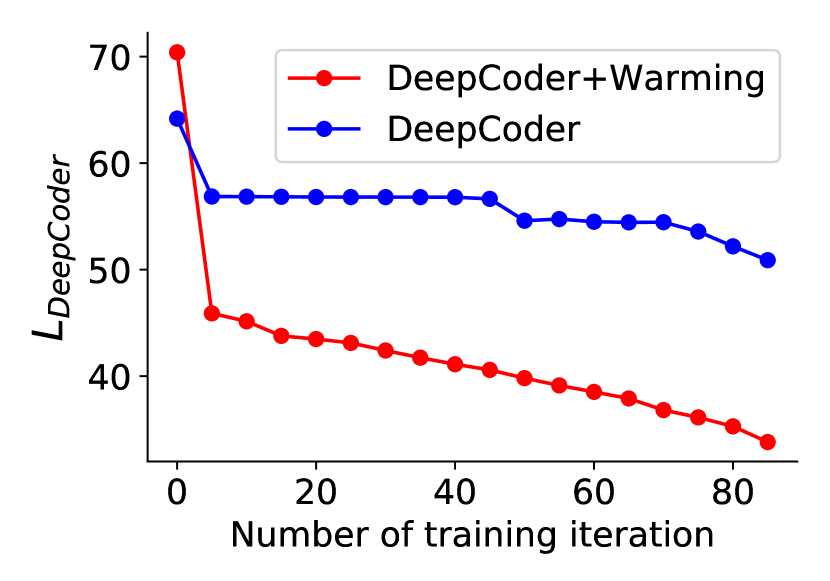
(c) Lower bounds

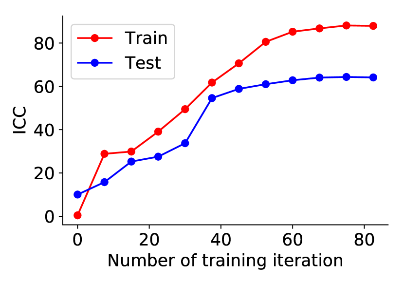
(d) ICC

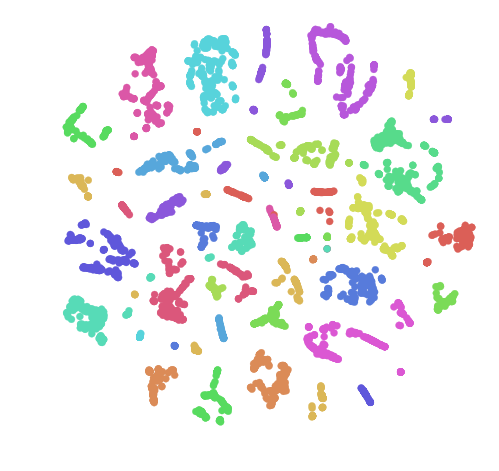
(e) Latent space $\boldsymbol{Z}_{0}$

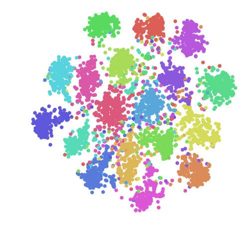
(f) Latent space $\boldsymbol{Z}_{1}$

Figure 3: FERA2015: (a) the MSE reconstruction error, (b) the NLPD of VO-GPAE, (c) the estimated variational lower bound per data point, (d) ICC for the AU intensity estimation, and the recovered latent spaces: $\boldsymbol{Z}_{0}$ (e), and $\boldsymbol{Z}_{1}$ (f).

Qualitative Results. Fig. (3) shows a summary of the model loss per iteration and the learned latent spaces for the two levels of the proposed DeepCoder, for the FERA2015 dataset. Fig. (3(a)) depicts the reconstruction error of the input images $X$ measured by (MSE) while Fig. (3(b)) visualizes the NLPD of the latent space $\boldsymbol{Z}_{0}$. While the reconstruction loss of the images converges quickly after five iteration, the NLPD of $\boldsymbol{Z}_{0}$ steadily decreases but needs 50 iterations to converge. The reason is the initialization. The weights for the latent space $\boldsymbol{Z}_{0}$ were initialized according to [13] which has proven to converge quickly, while VO-GPAE was initialized by drawing randomly from a normal distribution. Thus, $\boldsymbol{Z}_{1}$ required more iterations to converge. In Fig. (3(c)), we compare the lower bounds with and without warming strategy (see Sec. (4.2)). As expected, without warming strategy, the lower bound gets stuck in a local minimum, while the warming strategy lead to a steady decrease in the bound value. From the latent spaces $\boldsymbol{Z}_{0}$ and $\boldsymbol{Z}_{1}$ in Fig. (3(e),3(f)), we observe that $\boldsymbol{Z}_{0}$ is clustered according to subjects, but still the subjects are scattered over the latent space (showing the model’s invariance to identity, as also shown in [6]). However, in $\boldsymbol{Z}_{1}$ space, the model fits each subject into a separate cluster. As evidenced by our results, this clustering of the subjects leads to more efficient features for AU intensity estimation. We attribute this to the fact that GPs do an efficient smoothing over the training subjects closest to the test subject in the learned subspace - evidencing the importance of addressing the subject differences using non-parametric models.

7 Conclusions

We proposed a novel deep probabilistic framework, DeepCoder, for learning of deep latent representations and simultaneous classification of multiple ordinal labels. We showed in the context of face analysis that the joint learning of parametric features, followed by learning of the non-parametric latent features and target classifier, results in improved performance on the target task achieved by the proposed semi-parametric DeepCoder. We showed that this approach outperforms parametric deep AEs, and the state-of-the-art models for AU intensity estimation.

References

- [1] A. Agresti. Analysis of ordinal categorical data. John Wiley & Sons, 2010.
- [2] P. Baldi. Autoencoders, unsupervised learning, and deep architectures. ICML, 27(37-50):1, 2012.
- [3] M. S. Bartlett, G. C. Littlewort, M. G. Frank, C. Lainscsek, I. R. Fasel, and J. R. Movellan. Automatic recognition of facial actions in spontaneous expressions. Journal of multimedia, 1(6):22–35, 2006.
- [4] S. R. Bowman, L. Vilnis, O. Vinyals, A. M. Dai, R. Jozefowicz, and S. Bengio. Generating sentences from a continuous space. arXiv preprint arXiv:1511.06349, 2015.
- [5] W. Chu and Z. Ghahramani. Gaussian processes for ordinal regression. In JMLR, pages 1019–1041, 2005.
- [6] W. S. Chu, F. D. la Torre, and J. F. Cohn. Learning spatial and temporal cues for multi-label facial action unit detection. In FG, pages 25–32, 2017.
- [7] D. Ciregan, U. Meier, and J. Schmidhuber. Multi-column deep neural networks for image classification. In CVPR, pages 3642–3649, 2012.
- [8] Z. Dai, A. Damianou, J. González, and N. Lawrence. Variational auto-encoded deep Gaussian processes. In ICLR, 2016.
- [9] A. Damianou, C. H. Ek, M. Titsias, and N. Lawrence. Manifold relevance determination. In ICML, pages 145–152, 2012.
- [10] A. Damianou and N. Lawrence. Semi-described and semi-supervised learning with Gaussian processes. In UAI, 2015.
- [11] P. Ekman, W. V. Friesen, and J. C. Hager. Facial action coding system. A Human Face, Salt Lake City, UT, 2002.
- [12] S. Eleftheriadis, O. Rudovic, M. P. Deisenroth, and M. Pantic. Variational gaussian process auto-encoder for ordinal prediction of facial action units. In ACCV, pages 154–170, 2016.
- [13] X. Glorot and Y. Bengio. Understanding the difficulty of training deep feedforward neural networks. In Aistats, volume 9, pages 249–256, 2010.
- [14] K. Gregor, I. Danihelka, A. Graves, D. J. Rezende, and D. Wierstra. Draw: A recurrent neural network for image generation. arXiv preprint arXiv:1502.04623, 2015.
- [15] A. Gudi, H. E. Tasli, T. M. den Uyl, and A. Maroulis. Deep learning based facs action unit occurrence and intensity estimation. In FG’W, 2015.
- [16] J. Hensman and N. D. Lawrence. Nested variational compression in deep gaussian processes. arXiv preprint arXiv:1412.1370, 2014.
- [17] S. Kaltwang, S. Todorovic, and M. Pantic. Latent trees for estimating intensity of facial action units. In CVPR, 2015.
- [18] M. Kan, S. Shan, H. Chang, and X. Chen. Stacked progressive auto-encoders (spae) for face recognition across poses. In CVPR, pages 1883–1890, 2014.
- [19] A. Kapoor and R. W. Picard. Multimodal affect recognition in learning environments. In ACM, pages 677–682, 2005.
- [20] V. Kazemi and J. Sullivan. One millisecond face alignment with an ensemble of regression trees. In CVPR, pages 1867–1874, 2014.
- [21] P. Khorrami, T. Paine, and T. Huang. Do deep neural networks learn facial action units when doing expression recognition? In ICCV’W, pages 19–27, 2015.
- [22] D. P. Kingma, S. Mohamed, D. J. Rezende, and M. Welling. Semi-supervised learning with deep generative models. In NIPS, pages 3581–3589, 2014.
- [23] D. P. Kingma and M. Welling. Auto-encoding variational Bayes. In ICLR, 2013.
- [24] T. N. Kipf and M. Welling. Variational graph auto-encoders. arXiv preprint arXiv:1611.07308, 2016.
- [25] A. Krizhevsky, I. Sutskever, and G. E. Hinton. Imagenet classification with deep convolutional neural networks. In NIPS, pages 1097–1105, 2012.
- [26] T. D. Kulkarni, W. F. Whitney, P. Kohli, and J. Tenenbaum. Deep convolutional inverse graphics network. In NIPS, pages 2539–2547, 2015.
- [27] A. B. L. Larsen, S. K. Sønderby, H. Larochelle, and O. Winther. Autoencoding beyond pixels using a learned similarity metric. arXiv preprint arXiv:1512.09300, 2015.
- [28] N. Lawrence. Probabilistic non-linear principal component analysis with Gaussian process latent variable models. JMLR, 6:1783–1816, 2005.
- [29] Q. V. Le. Building high-level features using large scale unsupervised learning. In ICASSP, pages 8595–8598, 2013.
- [30] M. Liu, S. Li, S. Shan, and X. Chen. Au-aware deep networks for facial expression recognition. In FG, pages 1–6, 2013.
- [31] Y. Liu, X. Hou, J. Chen, C. Yang, G. Su, and W. Dou. Facial expression recognition and generation using sparse autoencoder. In SMARTCOMP, pages 125–130, 2014.
- [32] S. Lucey, A. B. Ashraf, and J. F. Cohn. Investigating spontaneous facial action recognition through aam representations of the face. INTECH Open Access Publisher, 2007.
- [33] M. Mahoor, S. Cadavid, D. Messinger, and J. Cohn. A framework for automated measurement of the intensity of non-posed facial action units. In CVPR, pages 74–80, 2009.
- [34] J. Masci, U. Meier, D. Cireşan, and J. Schmidhuber. Stacked convolutional auto-encoders for hierarchical feature extraction. In International Conference on Artificial Neural Networks, pages 52–59. Springer, 2011.
- [35] S. M. Mavadati, M. H. Mahoor, K. Bartlett, P. Trinh, and J. F. Cohn. Disfa: A spontaneous facial action intensity database. TAC, pages 151–160, 2013.
- [36] J. Nicolle, K. Bailly, and M. Chetouani. Facial action unit intensity prediction via hard multi-task metric learning for kernel regression. In FG, pages 1–6, 2015.
- [37] Z. Niu, M. Zhou, L. Wang, X. Gao, and G. Hua. Ordinal regression with multiple output cnn for age estimation. In CVPR, 2016.
- [38] T. Raiko, H. Valpola, M. Harva, and J. Karhunen. Building blocks for variational bayesian learning of latent variable models. JMLR, 8:155–201, 2007.
- [39] C. Rasmussen and C. Williams. Gaussian processes for machine learning, volume 1. MIT Press Cambridge, MA, 2006.
- [40] D. J. Rezende, S. Mohamed, and D. Wierstra. Stochastic backpropagation and approximate inference in deep generative models. In ICML, pages 1278–1286, 2014.
- [41] G. Sandbach, S. Zafeiriou, and M. Pantic. Markov random field structures for facial action unit intensity estimation. In ICCV’W, pages 738–745, 2013.
- [42] P. E. Shrout and J. L. Fleiss. Intraclass correlations: uses in assessing rater reliability. Psychological bulletin, 86(2):420, 1979.
- [43] K. Simonyan and A. Zisserman. Very deep convolutional networks for large-scale image recognition. CoRR, abs/1409.1556, 2014.
- [44] J. Snoek, R. P. Adams, and H. Larochelle. Nonparametric guidance of autoencoder representations using label information. JMLR, 13(Sep):2567–2588, 2012.
- [45] K. Sohn, H. Lee, and X. Yan. Learning structured output representation using deep conditional generative models. In NIPS, pages 3483–3491, 2015.
- [46] C. K. Sønderby, T. Raiko, L. Maaløe, S. K. Sønderby, and O. Winther. Ladder variational autoencoders. In NIPS, pages 3738–3746, 2016.
- [47] Y. Sun, X. Wang, and X. Tang. Deep learning face representation from predicting 10,000 classes. In CVPR, pages 1891–1898, 2014.
- [48] C. Szegedy, A. Toshev, and D. Erhan. Deep neural networks for object detection. In NIPS, pages 2553–2561, 2013.
- [49] M. K. Titsias and N. D. Lawrence. Bayesian gaussian process latent variable model. In AISTATS, volume 9, pages 844–851, 2010.
- [50] M. F. Valstar, T. Almaev, J. M. Girard, G. McKeown, M. Mehu, L. Yin, M. Pantic, and J. F. Cohn. Fera 2015-second facial expression recognition and analysis challenge. In FG, volume 6, pages 1–8, 2015.
- [51] A. van den Oord, N. Kalchbrenner, L. Espeholt, O. Vinyals, A. Graves, et al. Conditional image generation with pixelcnn decoders. In NIPS, pages 4790–4798, 2016.
- [52] P. Vincent, H. Larochelle, Y. Bengio, and P.-A. Manzagol. Extracting and composing robust features with denoising autoencoders. In ICML, pages 1096–1103, 2008.
- [53] P. Vincent, H. Larochelle, I. Lajoie, Y. Bengio, and P.-A. Manzagol. Stacked denoising autoencoders: Learning useful representations in a deep network with a local denoising criterion. JMLR, 11:3371–3408, 2010.
- [54] R. Walecki, O. Rudovic, V. Pavlovic, and M. Pantic. Copula ordinal regression for joint estimation of facial action unit intensity. In CVPR, pages 4902–4910, 2016.
- [55] R. Walecki, O. Rudovic, V. Pavlovic, B. Schuller, and M. Pantic. Deep structured learning for facial action unit intensity estimation. In CVPR, 2017.
- [56] Y. Zhang, R. Liu, S. Zhang, and M. Zhu. Occlusion-robust face recognition using iterative stacked denoising autoencoder. In NIPS, pages 352–359, 2013.
- [57] K. Zhao, W.-S. Chu, and H. Zhang. Deep region and multi-label learning for facial action unit detection. In CVPR, pages 3391–3399, 2016.