High-Quality Correspondence and Segmentation Estimation
for Dual-Lens Smart-Phone Portraits

Abstract

Estimating correspondence between two images and extracting the foreground object are two challenges in computer vision. With dual-lens smart phones, such as iPhone 7Plus and Huawei P9, coming into the market, two images of slightly different views provide us new information to unify the two topics. We propose a joint method to tackle them simultaneously via a joint fully connected conditional random field (CRF) framework. The regional correspondence is used to handle textureless regions in matching and make our CRF system computationally efficient. Our method is evaluated over 2,000 new image pairs, and produces promising results on challenging portrait images.

1 Introduction

It is convenient now to capture and share photos. It is reported that over one billion new images [24, 36] are shared every day over Internet and most of them are portraits [30, 18]. With the production of new dual-lens smart phones, a special way for two-image capturing becomes available for common users, which actually provides more intriguing information for many photo-related applications.

It seems a well-studied problem in computer vision that the two-camera output can be used to estimate depth with pixel correspondence established by optical flow estimation [19, 49] or stereo matching [41, 33]. Meanwhile it is also known in this community that producing pixel-level-accurate results is still difficult due primarily to diverse and complex content, textureless regions, noise, blur, occlusion, etc. An example is shown in Figure 1 where (a) and (e) are the input from a dual-lens camera. (b) and (c) show optical flow estimates of MDP [49] and LDOF [11] where errors are clearly noticeable. These types of errors are actually common when applying low-level image matching.

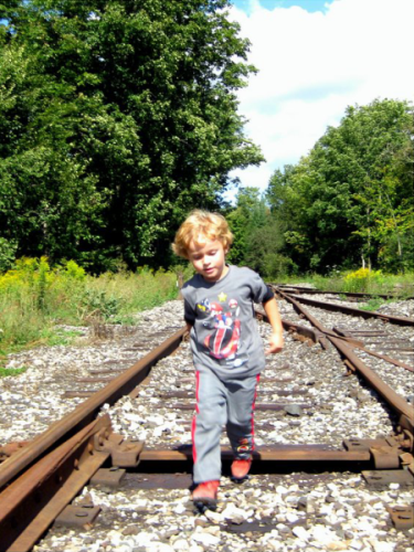
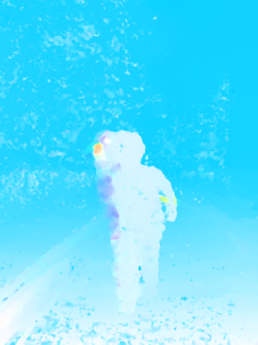
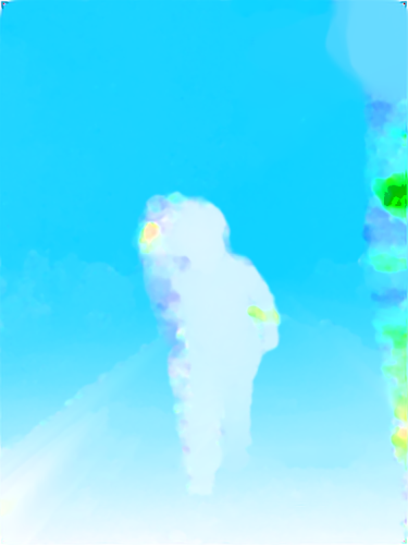
(a) Reference	(b) MDP Flow	(c) LDOF Flow	(d) Our Refined
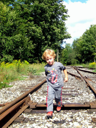
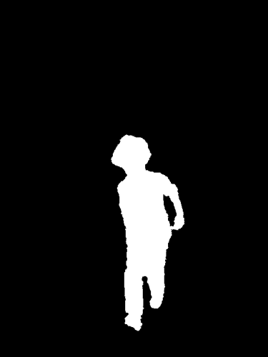
(e) Input	(f) FCN Segmentation	(g) CRFasRNN Segmentation	(h) Our Refined

Figure 1: Optical flow and semantic segmentation on dual-lens images. (a) and (e) are the input. (b) and (c) show MDP [49] and LDOF [11] estimates respectively. (f) is the FCN [29] segmentation result and (g) is the CRFasRNN [52] result. (d) and (h) are our estimated correspondence and segmentation respectively.

In this paper, we exploit extra information in dual-lens images to tackle this challenging problem on portraits. We incorporate high-level human-body clues in pixel correspondence estimation and propose a joint scheme to simultaneously refine pixel matching and object segmentation.

Analysis of Correspondence Estimation   Dual-lens images could be unrectified and with different resolutions. We thus resort to optical flow estimation instead of stereo matching for correspondence estimation. As briefly discussed above, several issues influence these methods even with robust outlier rejection schemes [10, 8, 44, 50]. Complicated nonlinear systems or discrete methods [23, 14, 5] have their respective optimization and accuracy limitations.

Difficulty of Semantic Segmentation   About semantic segmentation, state-of-the-art methods are based on fully convolutional networks (FCN) [29], which generate an per-pixel prediction score on all classes. Hierarchical convolution, pooling, rectification and deconvolution layers are adopted in the network. Even this advanced technique, semantic segmentation is still a challenging problem in terms of creating very accurate object boundaries. For the example shown in Figure 1(f), the small background area near the boy’s left arm is labeled as foreground. Although CRFs are applied to incorporate original image structure [52, 13], improvement is limited as shown in (g) [52]. The reason is that the CNNs predicted score is already wrong in this case.

Our Approach and Contribution   We propose a joint update method for portrait photos, taking initialization of simple optical flow estimates and FCN [29] segments. Then we form a joint fully connected conditional random fields (CRF) model to incorporate mutual information between correspondence and segmentation features. To make optimization tractable, we propose regional correspondence to greatly reduce CRF solution space. As a result, less then $40$ labels are produced for effective inference. Our method also handles textureless and outlier regions to improve estimation. To evaluate our approach, we collect 2,000 image pairs with labeled segmentation and correspondence. Our experiment shows that this method notably improves the accuracy compared with previous optical flow estimation and semantic segmentation approaches respectively.

2 Related Work

We briefly review optical flow estimation and image segmentation methods. Since both areas involve large sets of prior work, we only select related methods for discussion.

Optical Flow Methods   For image pairs captured in the same scene with intensity or gradient constancy, their correspondence can be computed with the variational model [19]. The involved data terms are used to satisfy color or gradient constancy [10, 12, 53]. Regularization terms can achieve piece-wise smooth results. The terms are usually formed by robust functions [10, 8, 44, 50].

Sparse descriptor matching is incorporated in the variational framework to handle large motion. Representative methods include those of [11] and [45]. The method of [49] fuses feature match in each coarse-to-fine pyramid scale. The variational model is nonlinear, which might be stuck in local minima when initialization is not appropriate.

Besides the variational model, nearest-neighbor field (NNF) strategies, such as PatchMatch [6, 7], are also applied. Chen et al. [14] estimated a coarse flow by PatchMatch and refined it by model fitting. To improve PatchMatch quality, Bao et al. [5] developed the edge-preserving patch similarity cost to search for the nearest neighbor. Recently, multi-scale NNF methods were proposed in [4].

The motion information is also applied to object segmentation as discussed in [47, 43, 40]. However, these methods need many frames to produce a reasonable result.

Image Segmentation Approaches   Interactive image segmentation was developed around a decade ago. These methods take user specified segment seeds for further optimization by graph cuts or CRF inference. Representative methods include graph-cut [9], Lazy Snapping [25], Grabcut [34], and paint selection [26, 1].

Recently, deep convolutional neural networks (CNNs) achieve great success in semantic segmentation. CNNs are applied mainly in two ways. The first is to learn image features and apply pixel classification [2, 31, 16]. The second line is to adopt an end-to-end trainable CNN model from input images to segmentation labels with the fully convolutional networks (FCN) [29].

To improve performance, DeepLab [13] and CRFasRNN [52] employed dense CRF to refine predicted score maps. Liu et al. [28] extended the general CRFs to deep parsing networks, which achieve state-of-the-art accuracy in the VOC semantic segmentation task [15]. Most CNNs are constructed hierarchically by convolution, pooling and rectification. They aim at challenging semantic segmentation with class labels. In terms of segmentation quality, interactive segmentation still perform better since users are involved.

Segmentation and Correspondence  To further improve correspondence estimation, methods of [38, 39, 40, 35, 20] utilized images layer or segment information. These methods model the correspondence in each layer and then use the correspondence to infer layer segmentation. A joint model with correspondence and layer estimation is formed, which is optimized by Expectation-Maximization (EM). Similar strategies were also employed in stereo matching [48]. It was found optimization of these models is time consuming and the segments (or layers) are not that semantically meaningful. Recently, Bai et al. [3] employed the semantic segmentation to refine the flow field; but no segment refinement by optical flow is considered.

3 Motivation of Our Approach

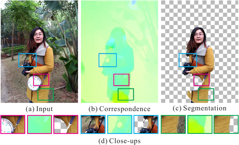
Figure 2: Discrepancy among input image, correspondence, and segmentation. (a) is the input image. (b) and (c) show the correspondence and segmentation maps respectively. (d) gives the close-ups.

Joint update of correspondence and segmentation is difficult because of the domain-level discrepancy among input image, estimated correspondence, and predicted segmentation. We show an example in Figure 2 where (a) is the input image, (b) is the correspondence result of Horn-Schunck flow method [19] and (c) shows the segmentation result by FCN [29]. The difference is on the following folds.

• Small Structure   Compared with interactive segmentation, semantic segmentation do not perform accurately as there exist many small structures in the image. On the contrary, optical flow methods work better on them. The blue rectangles in Figure 2(d) show the difference.

• Human Belonging and Accessories   Belonging and accessories on human bodies are excluded when performing classification, as people and other objects are separate into different categories. An example is shown in red rectangles in Figure 2(d) where the bag is excluded. It is not ideal for portrait images where accessories are part of human bodies.

• Textureless Regions   Correspondence estimation methods may fail in textureless regions. However, segmentation is less sensitive to them (see green patches in Figure 2(d)).

• Complex Background   Complex image background incurs extra difficulty for these methods, which will be detailed later.

These discrepancies show that joint refinement is nontrivial for fusion of different-domain information. Further, the large solution space with continuous correspondence makes refinement intractable. Our method splits the large solution space into several regionally accurate parts. With the new form, we achieve the goal via an efficient fully connected CRF model with a small number of labels.

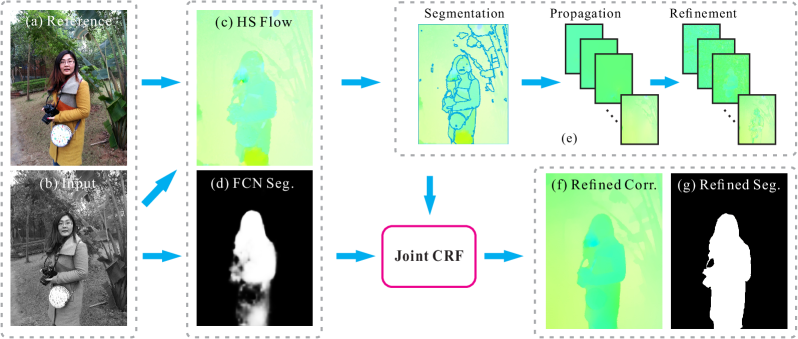
Figure 3: Illustration of our method. (a) and (b) are the reference and input images respectively. (c) and (d) are the Horn-Schunck flow [19] and FCN [29] segmentation results. (e) shows our regional correspondence. (f) and (g) are the refined results by our joint CRF model.

4 Our Approach

We estimate pixel correspondence $w$ between images $I_{1}$ and $I_{2}$ captured from a dual-lens smart-phone. Denoting by $p$ the pixel coordinate, displacement $w_{p}$ is to let pixel $p$ in $I_{1}$ correspond to $p+w_{p}$ in $I_{2}$. Besides estimating the correspondence $w$, we also aim for inferring portrait segmentation mask $m$, where $m_{p}=1$ indicates the person (i.e., foreground) and $m_{p}=0$ means background.

We construct a joint CRF model. As illustrated in Figure 3, our method starts from fast Horn-Schunck flow [19] and FCN segmentation [29] results. We first estimate regional correspondence for initialization and then form the joint updating scheme.

4.1 Regional Correspondence

Image correspondence is estimated regarding image content. To simplify computation, we adopt regional correspondence as shown in Figure 3(e). Regional correspondence is a set of correspondence maps denoted as $\{w^{i}|i=1,...N\}$ where $N$ is number of estimated regional correspondence. For each $w^{i}$, there exist some regions whose correspondence is accurate. Thus, the final correspondence map $w$ can be computed by a labeling process considering matching error and correspondence field smoothness. There are mainly two advantages of the regional correspondence.

• Initialization can be set appropriately for each regional correspondence to avoid the local minimum problem.

• Refinement can be achieved by regional correspondence selection to save much computation time.

Determining Regional Correspondence   We compute regional correspondence by weighted-median-filter-refined [51] Horn-Schunck flow as shown in Figure 3(c). The flow field is partitioned into regions according to motion boundary using the method of [46] according to color and flow features. Regions with similar flow are merged while those completely different from neighboring regions are discarded as outliers. We apply the very fast convolutional pyramid [17] to propagate flow to the whole image. The propagated regional correspondence labels the final result by fusion [49].

To improve sub-pixel accuracy, we refine each regional correspondence by the variational framework [10]. It, in general, can only improve accuracy near edges but not reliable correspondence for textureless regions, as the data term constraint is not discriminative enough. We thus only update the regional correspondence in the finest scale.

Analysis   Correspondence propagation is important to handle textureless regions. We show an example in Figure 4. For the textureless region between the arms in (a), flow estimation is erroneous as shown in (b). The PatchMatch-based method [5] works better in this region but presents errors in other area as shown in (c). Our estimate in (d) is from the regional correspondence by fusion [49], which achieves overall better quality. The reason is that background-propagated regional correspondence gives extra information. In addition, the number of partitioned regions is small due to sparsity of image content. In our experiments, $10$ correspondence regions are enough to produce usable results.

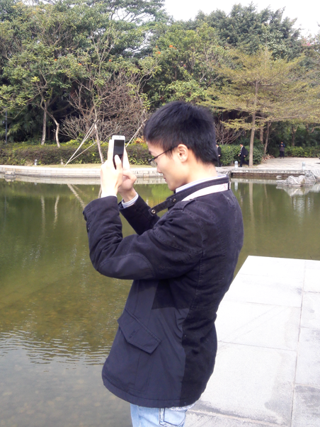
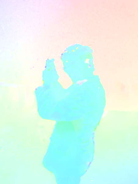
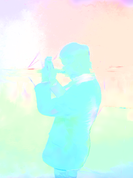
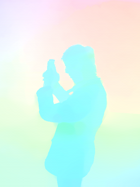
(a) Input	(b) MDP	(c) EPPM	(d) Ours

Figure 4: Correspondence estimation in textureless regions. (a) shows the input with textureless regions. (b-c) are MDP [49] and EPPM [5] flow estimates respectively. (d) is our result.

4.2 Joint Refinement Model

With regional correspondence $w^{i}$ and FCN predicted initial segmentation as shown in Figure 3(e) and (d), we adopt a fully connected CRF to improve them. Our model is formulated as

$$E(z)=\sum_{p\in\mathcal{V}}\psi_{d}(z_{p})+\sum_{p\in\mathcal{V}}\sum_{q\in\mathcal{E}_{p}}\psi_{s}(z_{p},z_{q}),$$ (1)

where $z$ is the variable set $z_{p}=[c_{p},m_{p}]$. $c_{p}$ denotes selection of the $c_{p}$th regional correspondence for pixel $p$ and $m_{p}$ is the segmentation label. $\psi_{d}$ and $\psi_{s}$ are the unary and pair-wise potentials. $\mathcal{V}$ is the set including all image pixels and $\mathcal{E}_{p}$ denotes image pixels for the fully connected CRF.

Joint Unary Potential $\psi_{d}(z_{p})$   The new part in this potential is to model the correspondence and segmentation interaction prior. It is defined as

$$\psi_{d}(z_{p})=\psi_{d}^{j}(c_{p},m_{p})+\alpha_{1}\psi_{d}^{c}(c_{p})+\alpha_{2}\psi_{d}^{m}(m_{p}),$$ (2)

where $\psi_{d}^{j}(c_{p},m_{p})$ models the joint potential between the $c_{p}$ and $m_{p}$ in pixel $p$. $\psi_{d}^{c}(c_{p})$ and $\psi_{d}^{m}(m_{p})$ are the potentials on the correspondence and segmentation likelihood respectively. $\alpha_{1}$ and $\alpha_{2}$ weight the three terms. A larger $\alpha_{1}$ emphasizes correspondence more and $\alpha_{2}$ influences segmentation likelihood.

We define the joint potential $\psi_{d}^{j}(c_{p},m_{p})$ according to the joint distribution

$$\psi_{d}^{j}(c_{p},m_{p})=-\log\big{(}h(w(c_{p}),m_{p})\big{)},$$ (3)

where $w(c_{p})$ is for the $c_{p}$th dominant correspondence for pixel $p$. $h(w,m)$ is the joint distribution between correspondence and segmentation. Since we have initialization correspondence and segmentation, we estimate $h(w,m)$ by computing the joint histogram.

For the regional correspondence unary potential $\psi_{d}^{c}(c_{p})$, we define it based on the matching cost. Motivated by optical flow intensity and gradient constancy, the potential is defined as

$$\psi_{d}^{c}(c_{p})=1-\exp\Big{(}{-\mu(I_{1},I_{2},w(c_{p}))}/{\sigma_{c}^{2}}\Big{)},$$ (4)

with

$$\mu(I_{1},I_{2},w(c_{p}))=\|I_{1,p}-I_{2,p+w(c_{p})}\|+\|\nabla I_{1,p}-\nabla I_{2,p+w(c_{p})}\|,$$

where $\mu$ computes the matching cost and $\nabla$ is the gradient operator. $\|\cdot\|$ computes the $L_{1}$ distance. $\sigma_{c}$ is the parameter controlling the matching cost. We set it to 0.2 in all our experiments.

We model the segmentation unary potential $\psi_{d}^{m}$ by the FCN predicted probability, which is defined as

$$\psi_{d}^{m}(m_{p})=-\log\big{(}S(m_{p})\cdot C(m_{p})\big{)},$$ (5)

where $S(m_{p})$ indicates the probability of pixel $p$ taking label $m_{p}$. We compute the probability using FCN predicted score after soft-max normalization. Rather than directly using original FCN model, we fine-turn it with our labeled portraits, which will be detailed later. $C(m_{p})$ is estimated from the foreground and background color model. With the initial segmentation mask, we fit a Gaussian mixture model (GMM) for color distributions of foreground and background as $h_{b}(x)$ and $h_{f}(x)$, similar to those of [26]. With the color models, we set $C(m_{p})=(1-m_{p})h_{b}(I_{1,p})+m_{p}h_{f}(I_{1,p})$. In all our experiments, we apply four Gaussian kernels for the background and six for foreground.

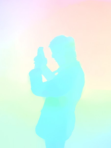
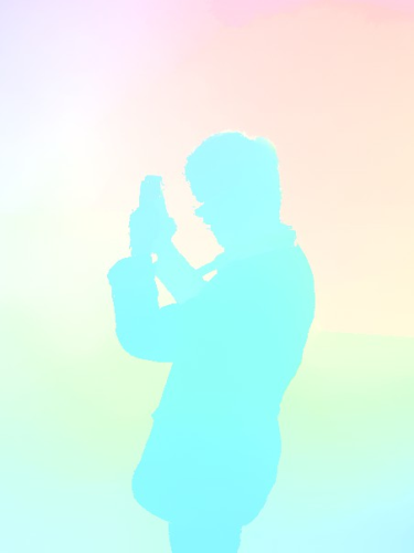
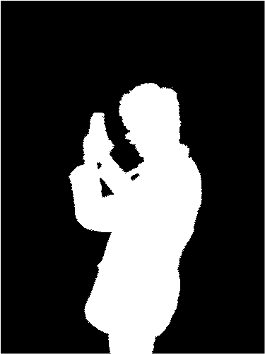
(a) Sep. Corr.	(b) Sep. Seg.	(c) Joint Corr.	(d) Joint Seg.

Figure 5: Comparison of separate and joint refinement on correspondence and segmentation using our CRF model. (a) and (b) are separately refined correspondence and segmentation results. (c) and (d) are the joint ones. The input is shown in Figure 4(a).

Joint Pair-Wise Term $\psi_{s}(z_{p},z_{q})$   The pair-wise term enforces regional flow selection and segmentation labeling for piece-wise smoothness. The correspondence and segmentation should have similar smooth property with close discontinuity in both images. To achieve it, the pair-wise term is formulated with the following three items.

$$\psi_{s}(z_{p},z_{q}) =\beta_{1}\psi_{s}^{c}(c_{p},c_{q})\psi_{s}^{m}(m_{p},m_{q})+\beta_{2}\psi_{s}^{c}(c_{p},c_{q})$$

$$+\beta_{3}\psi_{s}^{m}(m_{p},m_{q}).$$ (6)

The first item is joint pair-wise smoothness between $c$ and $m$. The goal is to force consistency between segmentation and correspondence. The last two items are the smoothness penalty in regional correspondence and segmentation labels respectively. $\beta_{1}$, $\beta_{2}$ and $\beta_{3}$ are the parameters. Similar to those of [25, 26, 21], we define them using the Potts model with bilateral weights as

$$\psi_{s}^{c}(c_{p},c_{q})=\delta(|c_{p}\!-\!c_{q}|)\cdot g(\|p-q\|,\|I_{1,p}\!-\!I_{1,q}\|,\sigma_{s},\sigma_{r}),$$

$$\psi_{s}^{m}(m_{p},m_{q})=\delta(|m_{p}\!-\!m_{q}|)\cdot g(\|p-q\|,\|I_{1,p}\!-\!I_{1,q}\|,\sigma_{s},\sigma_{r}),$$ (7)

where $\delta(x)$ is zero when $x$ is zero and is one otherwise. $g(x,y,\sigma_{s},\sigma_{r})$ is the bilateral weight function defined as $\exp({-x^{2}}/{\sigma_{s}^{2}}-y^{2}/\sigma_{r}^{2})$. The weight enforces neighboring pixels with similar color to select the same label in correspondence and segmentation space. $\sigma_{s}$ and $\sigma_{r}$ are the spatial and range parameters, which have the same influence as those in bilateral filter [42].

4.3 Inference

The objective function defined in Eq. (1) is an $NP$-hard problem on two sets of valuables $c$ and $m$. To efficiently infer them, we separate the system into two sub ones on $c$ and $m$ and alternatively update estimation.

• Given correspondence $c^{t}$, we optimize segment $m^{t}$.

• With updated segmentation $m^{t}$, we solve for $c^{t+1}$.

$t$ indexes iterations. The two sub-problems can be solved efficiently by mean field approximation [22]. In our experiments, 3-4 iterations are enough to get satisfying results.

4.4 Analysis

Why Joint Form?   The proposed joint model for correspondence and segmentation refinement makes use of correspondence labeling and segmentation. We compare it with separately processing correspondence and segmentation. In Eq. (1), the joint model degenerates to independent refinement when omitting all terms with respect to $c_{p}$ and $m_{p}$ respectively. We evaluate these models, and show results in Figure 5. It is noticeable that separately refining labels performs less well than our current system. Estimation of correspondence and segmentation can benefit each other via utilizing their mutual information.

Fully Connected CRF   Compared with general MRF, which uses only 4- or 8-neighbor smoothness terms, the fully connected CRF has the ability to label a very small region if it is globally distinct. To illustrate it, we show a comparison in Figure 6. For the results in (a) and (b), our model with the MRF term cannot correctly obtain the arm area because the region is very small. In contrast, our method is based on fully connected CRF and can handle such cases, as shown in (c) and (d).

Difference from Previous Approaches   Our method automatically refines semantic segmentation and correspondence estimation. Methods of [38, 39, 40] applied the layer information to higher quality correspondence inference. But no semantic object information is applied. Method of [3] exploited segmentation to help correspondence estimation. However, segmentation results are not refined in following processing. In addition, approach of [35] aims to model motion patterns for objects while ours is to simultaneously and effectively refine human segmentation and dual-lens correspondence.

(a) MRF Corr.	(b) MRF Seg.
(c) CRF Corr.	(d) CRF Seg.

Figure 6: Comparison of MRF and fully connected CRF. (a) and (b) are the results with the MRF pair-wise term. (c) and (d) are the results with our fully connected CRF term. The input image is shown in Figure 1.

5 Evaluation and Experiments

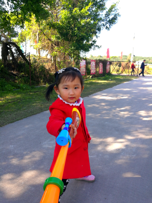
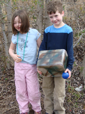
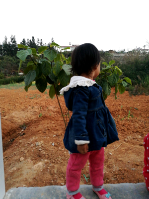
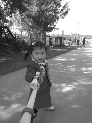
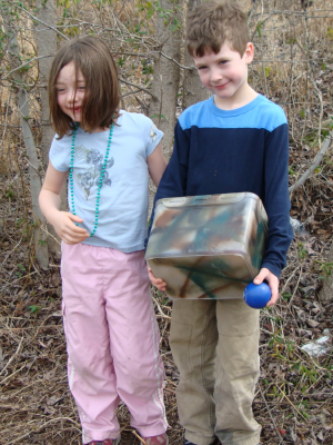
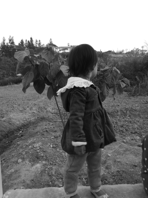
Figure 7: Our dual-lens image examples. The images in the top row are from the left camera and the bottom ones are from the right camera of Huawei P9.

We collected dual-lens portrait images with a Huawei P9 smart phone. We also search the data from Flickr with key words “stereo” and “3D image”. A few examples are shown in Figure 7. We select persons with a large variety in terms of age, gender, clothing, accessory, hair style and head position. Image background is with diverse structure regarding locations of indoor and outdoor scenes, weather, shadow, etc. All our captured images are with resolution $3968\times 2976$. Between the two captured images, one is with color and the other is grayscale because of the special camera setting. We denote the color image as reference and the grayscale one as input. Portrait areas are cropped and resized to $1200\times 800$. $2,000$ portrait image pairs are collected, which include 1,850 captured ones and 150 downloaded from Flickr.

With the selected dual-lens portrait images, we first label the human body segments in the color reference image using Photoshop quick selection tool [1] and take them as portrait segment ground truth.

Since it is very difficult to achieve accurate image correspondence, we fuse different-algorithm results with user interaction. First, we obtain correspondence results using state-of-the-art optical flow methods MDP [49], DeepFlow [45], EPPM [5], and LDOF [11]. For each method, we choose eight groups of parameter values and finally get 32 correspondence maps for each image pair. Second, we select the best correspondence from the 32 candidates using the method of [23]. Third, we label unmatched area with user interaction and apply flow completion [27]. Finally, we take edited correspondence maps as ground truth for all portrait image pairs. We split the 2,000 pairs into 1,800 pairs for training and 200 for evaluation.

5.1 Comparison and Evaluation

In terms of the system structure, we compute initial Horn-Schunck optical flow using the code of [37] with default parameters. Fast weighted median filter [51] is then applied to smooth it. For semantic segmentation initialization, we changed the original FCN-8s model to 2 outputs, which are the background and foreground similar to that of [36]. Then the model is fine- tuned using our training data based on the original FCN-8s model. The fine-tuning process can improve segmentation accuracy, to be shown below. For the joint update model, we set $\alpha_{1}$ and $\alpha_{2}$ both to 1.5. $\beta_{1}$, $\beta_{2}$ and $\beta_{2}$ are all set to3 by default. $\sigma_{s}$ ranges from 10 to 20 and $\sigma_{r}$ is set around $0.2$. The running time of our method for a $600\times 800$ image pair is 16.63 seconds on an Intel Core-i7 CPU PC without any GPU acceleration. In all our experiments, the results are generated in 3 iterations.

Evaluation on Our Data   With our data, we evaluate the methods quantitatively in terms of segmentation and correspondence accuracy. We compare the person segmentation with state-of-the-art methods FCN [29], DeepLab [13] and CRFasRNN [52] using the author published model. Besides directly applying the original 20-class object model, we change each model to 2-class output with portrait and background. These methods are all fine-tuned with our portrait data. We define these fine-tuned models as “FCN-portrait”, “DeepLab-portrait” and “CRFasRNN-portrait”.

The results are reported in Table 1 where we apply the intersection-over-union (IoU) to measure the segmentation accuracy with respect to ground truth. The table shows that the three 20-class object segmentation models achieve around 80% IoU accuracy. By updating the models to 2-class output and further fine-tuning them by our portrait data, their accuracy is improved by about 4%. We also test our model only updating the segmentation, which achieved very limited improvement. Our joint model presents the best performance, bearing out the effectiveness of jointly refining correspondence and segmentation.

Methods	Mean IoU(%)
FCN [29]	79.51
DeepLab [13]	80.09
CRFasRNN [52]	80.23
FCN-portrait	83.90
DeepLab-portrait	84.01
CRFasRNN-portrait	84.19
Ours-separate	84.32
Ours	88.33

Table 1: Comparison of segmentation results on our data. “FCN-portrait”, “DeepLab-portrait” and “CRFasRNN-portrait” denote fine-tuned models using our labeled image data. “Ours-separate” is the model only updating segmentation.

Methods	AEPE	AAE
HS Flow [37]	13.66	10.48
TV-L1 Flow [10]	10.01	8.52
LDOF Flow [11]	8.32	7.81
MDP Flow [49]	8.23	7.96
EPPM Flow [5]	11.74	9.05
DeepFlow [45]	7.87	6.81
EpicFlow [32]	8.11	7.49
Ours-separate	8.03	7.45
Ours	5.29	5.91

Table 2: Comparison of correspondence results on our data. We calculate the average end point error (AEPE) and average angular error (AAE).

We compare our methods with other dense correspondence estimation approaches, including Horn-Schunck [37], TV-L1 [10], MDP [49], DeepFlow [45], LDOF [11], EpicFlow [32], and EPPM [5]. Evaluation results are given in Table 2. Compared with the variational model without feature matching constraints, such as HS and TV-L1 model, the methods LDOF, MDP, DeepFlow, and EpicFlow achieve better performance. We also evaluate our model by only refining the correspondence. The result is much improved over the initial HS flow. Our final joint model yields the best performance among all matching methods.

Visual Comparison   As shown in Figure 8, we compare our method with previous matching methods MDP [49], LDOF [11], DeepFlow [45] and semantic segmentation approaches FCN [29], FCN-portrait, and CRFasRNN [52]. Our method also notably improves the matching accuracy in human body boundaries and textureless regions. By utilizing the reliable correspondence information, decent performance is accomplished for portrait segmentation.

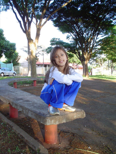
(a) Input	(b) MDP Flow	(c) LDOF Flow	(d) DeepFlow	(e) Our Corr.
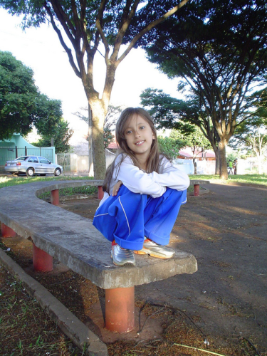
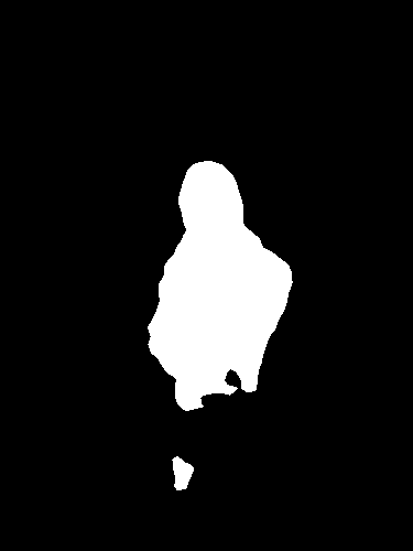
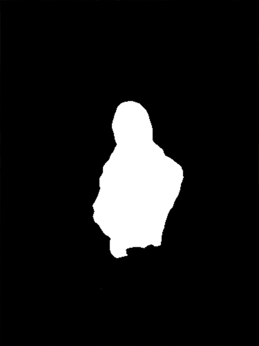
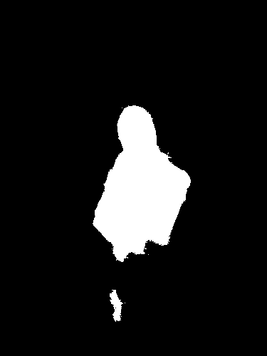
(f) Reference	(g) FCN	(h) FCN-portrait	(i) CRFasRNN	(j) Our Seg.
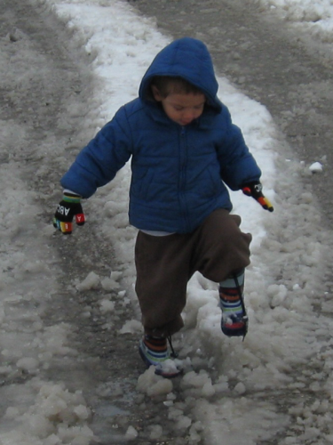
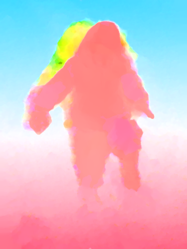
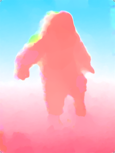
(a) Input	(b) MDP Flow	(c) LDOF Flow	(d) DeepFlow	(e) Our Corr.
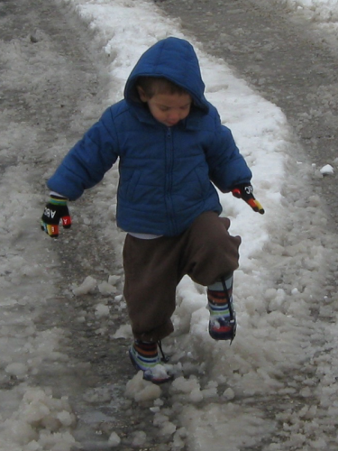
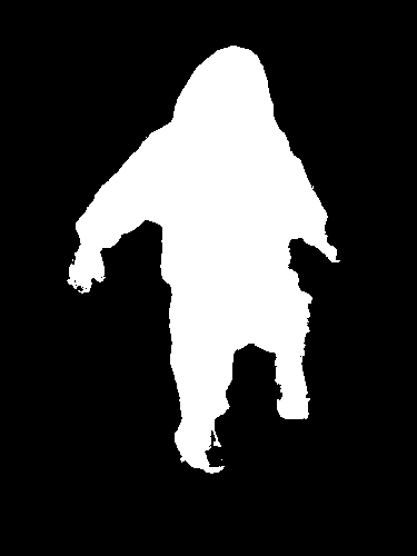
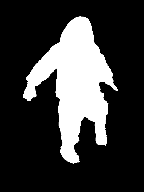
(f) Reference	(g) FCN	(h) FCN-portrait	(i) CRFasRNN	(j) Our Seg.

Figure 8: Visual comparisons of different segmentation and correspondence estimation methods. (a) and (f) are the input and reference images respectively. (b-e) are the correspondence estimated by MDP [49], LDOF [11] and DeepFlow [45] respectively. (g-i) are the FCN, FCN-portrait and CRFasCNN segmentation results respectively. (e) is our correspondence result and (f) is our segmentation result.

Regional Correspondence Effectiveness   Our regional correspondence estimation greatly speeds up the labeling process and increases accuracy by resolving the textureless issue. To verify it, we compare our method with the non-regional estimation scheme, which is to set $w^{i}$ into discrete constant maps covering all possible displacements. We use 500 uniformly sampled values from $[-50,50]\times[50,50]$ to get all $w^{i}$s. As reported in Table 3, with our regional correspondence, the method is 10 times faster and is also more accurate in terms of the AEPE measure.

Methods	Accuracy (AEPE)	Running Time (Seconds)
without RC	6.45	186.3
with RC	5.29	16.63

Table 3: Performance of our regional correspondence estimation. “RC” denotes the regional correspondence.

6 Conclusion

We have proposed an effective method for joint correspondence and segmentation estimation for portrait photos. Our method still has the following limitations. First, our approach may fail when the image contains many persons – our training data does not include such cases. Second, the extra low-level imaging problems such as highlight, heavy noise, and burry could degrade our method for reliable correspondence and segmentation estimation. Our future work will be to deal with these issues with more training data and enhanced models.

References

- [1] ADOBE SYSTEMS. Adobe photoshop cc 2015 tutorial.
- [2] P. Arbelaez, B. Hariharan, C. Gu, S. Gupta, L. D. Bourdev, and J. Malik. Semantic segmentation using regions and parts. In CVPR, pages 3378–3385, 2012.
- [3] M. Bai, W. Luo, K. Kundu, and R. Urtasun. Exploiting semantic information and deep matching for optical flow. In ECCV, pages 154–170, 2016.
- [4] C. Bailer, B. Taetz, and D. Stricker. Flow fields: Dense correspondence fields for highly accurate large displacement optical flow estimation. In ICCV, 2015.
- [5] L. Bao, Q. Yang, and H. Jin. Fast edge-preserving patchmatch for large displacement optical flow. IEEE Transactions on Image Processing, 23(12):4996–5006, 2014.
- [6] C. Barnes, E. Shechtman, A. Finkelstein, and D. B. Goldman. Patchmatch: a randomized correspondence algorithm for structural image editing. ACM Trans. Graph., 28(3), 2009.
- [7] C. Barnes, E. Shechtman, D. B. Goldman, and A. Finkelstein. The generalized patchmatch correspondence algorithm. In ECCV, pages 29–43, 2010.
- [8] M. J. Black and P. Anandan. The robust estimation of multiple motions: Parametric and piecewise-smooth flow fields. Computer Vision and Image Understanding, 63(1):75–104, 1996.
- [9] Y. Y. Boykov and M.-P. Jolly. Interactive graph cuts for optimal boundary & region segmentation of objects in nd images. In ICCV, volume 1, pages 105–112, 2001.
- [10] T. Brox, A. Bruhn, N. Papenberg, and J. Weickert. High accuracy optical flow estimation based on a theory for warping. In ECCV, pages 25–36, 2004.
- [11] T. Brox and J. Malik. Large displacement optical flow: descriptor matching in variational motion estimation. IEEE Trans. Pattern Anal. Mach. Intell., 33(3):500–513, 2011.
- [12] A. Bruhn and J. Weickert. Towards ultimate motion estimation: Combining highest accuracy with real-time performance. In ICCV, pages 749–755, 2005.
- [13] L. Chen, G. Papandreou, I. Kokkinos, K. Murphy, and A. L. Yuille. Semantic image segmentation with deep convolutional nets and fully connected crfs. ICLR, 2014.
- [14] Z. Chen, H. Jin, Z. Lin, S. Cohen, and Y. Wu. Large displacement optical flow from nearest neighbor fields. In CVPR, pages 2443–2450, 2013.
- [15] M. Everingham, L. J. V. Gool, C. K. I. Williams, J. M. Winn, and A. Zisserman. The pascal visual object classes (VOC) challenge. International Journal on Computer Vision, 88(2):303–338, 2010.
- [16] C. Farabet, C. Couprie, L. Najman, and Y. LeCun. Learning hierarchical features for scene labeling. IEEE Trans. Pattern Anal. Mach. Intell., 35(8):1915–1929, 2013.
- [17] Z. Farbman, R. Fattal, and D. Lischinski. Convolution pyramids. ACM Trans. Graph., 30(6):175, 2011.
- [18] M. Hall. Family albums fade as the young put only themselves in picture.
- [19] B. K. P. Horn and B. G. Schunck. Determining optical flow. Artif. Intell., 17(1-3):185–203, 1981.
- [20] J. Hur and S. Roth. Joint optical flow and temporally consistent semantic segmentation. In ECCV Workshops, pages 163–177, 2016.
- [21] P. Krähenbühl and V. Koltun. Efficient inference in fully connected crfs with gaussian edge potentials. In NIPS, pages 109–117, 2011.
- [22] P. Krähenbühl and V. Koltun. Efficient inference in fully connected crfs with gaussian edge potentials. In NIPS, pages 109–117, 2011.
- [23] V. Lempitsky, S. Roth, and C. Rother. Fusionflow: Discrete-continuous optimization for optical flow estimation. In CVPR, 2008.
- [24] E. LePage. A long list of instagram statistics and facts (that prove its importance), 2015.
- [25] Y. Li, J. Sun, C. Tang, and H. Shum. Lazy snapping. ACM Trans. Graph., 23(3):303–308, 2004.
- [26] J. Liu, J. Sun, and H. Shum. Paint selection. ACM Trans. Graph., 28(3), 2009.
- [27] S. Liu, L. Yuan, P. Tan, and J. Sun. Steadyflow: Spatially smooth optical flow for video stabilization. In CVPR, pages 4209–4216, 2014.
- [28] Z. Liu, X. Li, P. Luo, C. C. Loy, and X. Tang. Semantic image segmentation via deep parsing network. In ICCV, pages 1377–1385, 2015.
- [29] J. Long, E. Shelhamer, and T. Darrell. Fully convolutional networks for semantic segmentation. CVPR, 2014.
- [30] J. Mick. HTC: 90% of phone photos are selfies, we want to own the selfie market.
- [31] M. Mostajabi, P. Yadollahpour, and G. Shakhnarovich. Feedforward semantic segmentation with zoom-out features. In CVPR, 2014.
- [32] J. Revaud, P. Weinzaepfel, Z. Harchaoui, and C. Schmid. Epicflow: Edge-preserving interpolation of correspondences for optical flow. In CVPR, pages 1164–1172, 2015.
- [33] C. Rhemann, A. Hosni, M. Bleyer, C. Rother, and M. Gelautz. Fast cost-volume filtering for visual correspondence and beyond. In CVPR, 2011.
- [34] C. Rother, V. Kolmogorov, and A. Blake. ”grabcut”: interactive foreground extraction using iterated graph cuts. ACM Trans. Graph., 23(3):309–314, 2004.
- [35] L. Sevilla-Lara, D. Sun, V. Jampani, and M. J. Black. Optical flow with semantic segmentation and localized layers. In CVPR, pages 3889–3898, 2016.
- [36] X. Shen, A. Hertzmann, J. Jia, S. Paris, B. Price, E. Shechtman, and I. Sachs. Automatic portrait segmentation for image stylization. In Eureographcis, 2016.
- [37] D. Sun, S. Roth, and M. J. Black. Secrets of optical flow estimation and their principles. In CVPR, pages 2432–2439, 2010.
- [38] D. Sun, E. B. Sudderth, and M. J. Black. Layered image motion with explicit occlusions, temporal consistency, and depth ordering. In NIPS, pages 2226–2234, 2010.
- [39] D. Sun, E. B. Sudderth, and M. J. Black. Layered segmentation and optical flow estimation over time. In CVPR, pages 1768–1775, 2012.
- [40] D. Sun, J. Wulff, E. B. Sudderth, H. Pfister, and M. J. Black. A fully-connected layered model of foreground and background flow. In CVPR, pages 2451–2458, 2013.
- [41] J. Sun, N. Zheng, and H.-Y. Shum. Stereo matching using belief propagation. IEEE Trans. Pattern Anal. Mach. Intell., 25(7):787–800, 2003.
- [42] C. Tomasi and R. Manduchi. Bilateral filtering for gray and color images. In ICCV, pages 839–846, 1998.
- [43] M. Unger, M. Werlberger, T. Pock, and H. Bischof. Joint motion estimation and segmentation of complex scenes with label costs and occlusion modeling. In CVPR, pages 1878–1885, 2012.
- [44] A. Wedel, C. Rabe, T. Vaudrey, T. Brox, U. Franke, and D. Cremers. Efficient dense scene flow from sparse or dense stereo data. In ECCV, pages 739–751, 2008.
- [45] P. Weinzaepfel, J. Revaud, Z. Harchaoui, and C. Schmid. DeepFlow: Large displacement optical flow with deep matching. In ICCV, 2013.
- [46] P. Weinzaepfel, J. Revaud, Z. Harchaoui, and C. Schmid. Learning to detect motion boundaries. In CVPR, pages 2578–2586, 2015.
- [47] Y. Weiss and E. H. Adelson. A unified mixture framework for motion segmentation: Incorporating spatial coherence and estimating the number of models. In CVPR, pages 321–326, 1996.
- [48] W. Xiong, H. Chung, and J. Jia. Fractional stereo matching using expectation-maximization. IEEE Trans. Pattern Anal. Mach. Intell., 31(3):428–443, 2009.
- [49] L. Xu, J. Jia, and Y. Matsushita. Motion detail preserving optical flow estimation. IEEE Trans. Pattern Anal. Mach. Intell., 34(9):1744–1757, 2012.
- [50] C. Zach, T. Pock, and H. Bischof. A duality based approach for realtime TV-L1 optical flow. Pattern Recognition, pages 214–223, 2007.
- [51] Q. Zhang, L. Xu, and J. Jia. 100+ times faster weighted median filter (WMF). In CVPR, pages 2830–2837, 2014.
- [52] S. Zheng, S. Jayasumana, B. Romera-Paredes, V. Vineet, Z. Su, D. Du, C. Huang, and P. H. S. Torr. Conditional random fields as recurrent neural networks. ICCV, 2015.
- [53] H. Zimmer, A. Bruhn, J. Weickert, B. R. Levi Valgaerts and, Agustín Salgado, and H.-P. Seidel. Complementary optic flow. In EMMCVPR, 2009.