Giant gigahertz optical activity in multiferroic ferroborate

Abstract

In contrast to well studied multiferroic manganites with a spiral structure, the electric polarization in multiferroic borates is induced within collinear antiferromagnetic structure and can easily be switched by small static fields. Because of specific symmetry conditions, static and dynamic properties in borates are directly connected, which leads to giant magnetoelectric and magnetodielectric effects. Here we prove experimentally that the giant magnetodielectric effect in samarium ferroborate SmFe₃(BO₃)₄  is of intrinsic origin and is caused by an unusually large electromagnon situated in the microwave range. This electromagnon reveals strong optical activity exceeding 120 degrees of polarization rotation in a millimeter thick sample.

I Introduction

Rapid progress of modern electronics requires a continuous search for new mechanisms of controlling electric and magnetic properties of materials. One of the promising recent developments targets materials with the magnetoelectric effect which allows to influence electric properties by magnetic field and magnetization by electric voltage fiebig_jpd_2005 ; ramesh_nmat_2007 ; eerenstein_nature_2006 ; tokura_science_2006 . In view of future applications, the absolute value of magnetoelectric coupling is of crucial importance. One newly discovered material class with record values of the magnetoelectric effect are rare-earth borates vasiliev_ltp_2006 ; kadomtseva_ltp_2010 ; liang_prb_2011 , RFe₃(BO₃)₄ and RAl₃(BO₃)₄ (R = rare earth ion). Especially in ferroborates with R = Sm, Ho colossal magnetic field-induced changes in the dielectric constant have been observed mukhin_jetpl_2011 ; chaudhury_prb_2009 exceeding $\Delta\varepsilon/\varepsilon\sim 300\%$. Up to now such unusually large changes in the dielectric constant were known to arise because of extrinsic effects, such as domain wall motion kagawa_prl_2009 or contact and grain boundary effects lunkenheimer_prb_2002 . In the case of SmFe₃(BO₃)₄  it has been suggested that an intrinsic magnetoelectric excitation may be responsible for the observed effects mukhin_jetpl_2011 ; kuzmenko_jetp_2011 . Such excitations in magnetoelectric materials are called electromagnons pimenov_jpcm_2008 ; sushkov_jpcm_2008 , and they are defined as magnetic excitations that interact with the electric component of electromagnetic radiation.

Although the existence of certain magnetoelectric modes in SmFe₃(BO₃)₄  may be expected from the basic arguments, all relevant frequency ranges except for the microwaves could be excluded in previous experiments. In this work we prove the existence of a magnetoelectric excitation at gigahertz frequencies. The observation of the electromagnon in SmFe₃(BO₃)₄  becomes possible because the eigenfrequency of the mode can be lifted to the millimeter-wave range by the external magnetic field. Because of the strong coupling of static and dynamic magnetoelectric properties in SmFe₃(BO₃)₄  giant controlled polarization rotation is demonstrated.

Magneto-optical effects in multiferroics represent an intensive and rapidly developing field of investigations. The examples include magnetic field-induced dichroism in the terahertz range pimenov_nphys_2006 ; kida_prb_2011 , controlled chirality bordacs_nphys_2012 , directional dichroism kezsmarki_prl_2011 ; takahashi_nphys_2012 ; takahashi_prl_2013 . Electric control of terahertz radiation is more difficult to realize and it has been recently demonstrated in the millimeter wave-range shuvaev_prl_2013 and by Raman scattering rovillain_nmat_2010 .

In ferroborates RFe₃(BO₃)₄ the unusual strength of the magnetoelectric coupling results from the presence of two magnetic subsystems: iron and rare-earth kadomtseva_ltp_2010 . Existing data suggest that the interaction between the two subsystems increases the magnetoelectric coupling in ferroborates by at least one order of magnitude zvezdin_jetpl_2006 . A distinctive feature of the borates is that their crystal structure is non-centrosymmetric which is in contrast to manganites with a perovskite-like structure (RMnO₃). This results in different symmetry conditions for magnetoelectric properties. In particular, in ferroborates electric polarization is induced by the external magnetic field or by collinear antiferromagnetic ordering of Fe-ions while in the manganites it appears only within non-centrosymmetric (cycloidal) antiferromagnetic ordering of Mn ions. The microscopic mechanism of magnetoelectricity in borates is still unknown. However, it seems to be clear that the same mechanism is responsible for static and dynamic magnetoelectric effects. This coupling promises desirable direct connection between static and gigahertz properties, which may open up novel applications such as new effective ways to control millimeter-wave light with external voltage or magnetic field. The connection described above differs considerably from that in rare-earth manganites. In manganites the static polarization is determined by Dzyaloshinski-Moriya coupling katsura_prl_2007 ; mostovoy_prl_2006 and the dynamic properties are mainly governed by the Heisenberg exchange mechanism aguilar_prl_2009 ; lee_prb_2009 . This incompatibility hampers the control of dynamic properties by static fields.

II Experimental

Spectroscopic experiments in the terahertz frequency range (40 GHz $<\nu<$ 1000 GHz) have been carried out in a Mach-Zehnder interferometer arrangement volkov_infrared_1985 which allows measurements of the amplitude and the phase shift in a geometry with controlled polarization of radiation. Theoretical transmittance curves shuvaev_sst_2012 for various geometries were calculated from the susceptibilities using Fresnel optical equations for the complex transmission coefficient and within the Berreman formalism berreman_josa_1972 . Details of the terahertz data processing are given in Appendix B. The experiments in external magnetic fields up to 7 T have been performed in a superconducting split-coil magnet with polypropylene windows. Static dielectric measurements have been done using commercial impedance analyzer equipped with a superconducting magnet. Large single crystals of SmFe₃(BO₃)₄, with typical dimensions of $\sim 1$ cm, have been grown by crystallization from the melt on seed crystals.

III Samarium Ferroborate

SmFe₃(BO₃)₄  contains two interacting localized magnetic subsystems given by Sm³⁺ and Fe³⁺ ions. The iron subsystem orders antiferromagnetically below $T_{N}=34~{}K$ with an easy-plane magnetic structure oriented perpendicularly to the trigonal c-axis. Although the Sm³⁺ moments play an important role in the magnetoelectric properties of SmFe₃(BO₃)₄, they probably do not order up to the lowest temperatures. The crystallographic structure of SmFe₃(BO₃)₄  is shown in Fig. 1a. SmFe₃(BO₃)₄  has a non-centrosymmetric trigonal structure with R32 space group vasiliev_ltp_2006 .

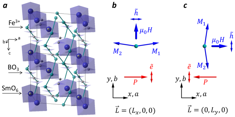
Figure 1: Magnetic structure of SmFe₃(BO₃)₄. a - Basic structural elements in SmFe₃(BO₃)₄. b - Orientation of Fe³⁺ magnetic moments and the excitation conditions of the magnetoelectric mode (electromagnon) in external magnetic fields parallel to the crystallographic $b(y)$-axis. c - changes in the magnetic structure and excitation conditions for $\mu_{0}H\|a(x)$-axis.

Static electric polarization in multiferroic ferroborates can be explained by symmetry arguments and by taking into account that Fe³⁺ moments are oriented antiferromagnetically within the crystallographic $ab$-plane zvezdin_jetpl_2005 ; zvezdin_jetpl_2006 . Within the topic of the present work the term governing the ferroelectric polarization along the $a$ and $b$-axis (or $x$ and $y$-axis, see Fig. 1a) is of basic importance. For the R32 space group of borates this term is given by

$$P_{x}\sim L_{x}^{2}-L_{y}^{2},\quad P_{y}\sim-2L_{x}L_{y}\ .$$ (1)

Here $L=M_{1}-M_{2}$ is the antiferromagnetic vector with $M_{1}$ and $M_{2}$ being the magnetic moments of two (antiferro-)magnetic Fe³⁺ sublattices. Full details of the symmetry analysis of the static magnetoelectric effects in SmFe₃(BO₃)₄  can be found in Refs. zvezdin_jetpl_2005 ; zvezdin_jetpl_2006 ; popov_prb_2013 .

Simple expression Eq. (1) allows to understand the behavior of static and dynamic properties in external magnetic fields. As shown in Fig. 1b, static magnetic field along the $y$-axis stabilizes the magnetic configuration with $L_{y}=0$ and $L_{x}\neq 0$. In agreement with Eq. (1) in this case the static polarization is oriented parallel to the a-axis. For magnetic fields along the $x$-axis and above the spin flop value $L_{x}=0$ and $L_{y}\neq 0$ which leads to antiparallel orientation of electric polarization with respect to the a-axis (Fig. 1c).

Details of the model analysis of the magnetoelectric modes in SmFe₃(BO₃)₄  are given in Appendix A. In brief, the magnetic and electric excitation channels are connected because of direct coupling of the antiferromagnetism and ferroelectricity. The low-frequency magnetoelectric mode of interest corresponds to oscillations of antiferromagnetic moment $L$ in the easy $ab$-plane. It can be excited either by an ac electric field with $e\bot P$ or by an ac magnetic field $h\bot M$. Here $P$ is the static electric polarization and $M\|\mu_{0}H$ is a weak field-induced ferromagnetic moment with $M\bot L$. Because electric polarization is directly coupled to the antiferromagnetic order, it becomes possible to excite the spin oscillations not only by an ac magnetic field but by an alternating electric field as well. The excitation conditions of the electromagnon strongly differ for two magnetic configurations given in Figs. 1b,c. In particular, the excitation conditions of the electromagnon for the configuration in Fig. 1c are given by $e\|b$ or $h\|b$. Therefore, for an ab-cut of SmFe₃(BO₃)₄  crystal we can selectively excite either electric ($e\|b$) or magnetic ($h\|b$) component of the electromagnon simply by rotating the polarization of the incident radiation.

The excitation conditions of the electromagnon change substantially if the static magnetic field is parallel to the $b$-axis as shown in Fig. 1b. In this case the external field stabilizes the configuration with magnetic moments parallel to the $a$-axis and with $L_{y}=0$. In agreement with Eq. (1), the static electric polarization is parallel to the $a$-axis. The excitation conditions of the electromagnon now changes to $e\|b$ and $h\|a$. Therefore, with this configuration of the magnetic moments and for an $ab$-cut sample the electric and magnetic excitation channels are either simultaneously active (for the polarization $e\|b,h\|a$) or they are both silent (for $e\|a,h\|b$).

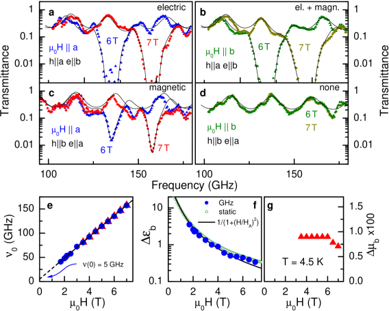
Figure 2: Selective excitation of electromagnon in SmFe₃(BO₃)₄. a-d - Transmittance spectra for two orientations of external magnetic field, $\mu_{0}H\|a$ (a,c) and $\mu_{0}H\|b$ (b,d). Different excitation conditions allow to selectively probe electric (a), magnetic (c), magnetoelectric (b), or silent (d) geometry. e - Magnetic field dependence of the electromagnon frequency. Circles - $\mu_{0}H\|a,h\|a,e\|b$, triangles - $\mu_{0}H\|a,h\|b,e\|a$, straight line is a linear fit to the resonance frequency with $\nu_{0}(0T)=5$ GHz. f,g - Field dependence of the electric and magnetic contribution of the electromagnon. Circles - electric contribution, red full triangles - magnetic contribution, green open triangles - static permittivity, solid line - model calculations.

IV Results and Discussion

Typical transmittance spectra of SmFe₃(BO₃)₄  in the frequency range of our spectrometer are shown in Figs.  2a-d. These results support the symmetry arguments given above and they can be consistently described by an electromagnon revealing an electric dipole moment parallel to the $b$-axis and with the magnetic dipole moment which can be switched between $h\|a$ and $h\|b$ depending on the orientation of the static magnetic field.

The eigenfrequency of the electromagnon in SmFe₃(BO₃)₄ in zero magnetic field is determined by the weak magnetic anisotropy in the basis $ab$-plane and is estimated as $\nu_{0}\approx 5$ GHz. This frequency increases roughly linearly with external magnetic field as demonstrated in Fig. 2e. Strong tunability of the electromagnon frequency in external fields makes multiferroic ferroborates an attractive material class for applications. As demonstrated in Fig. 2f and in agreement with the model given in Appendix A, the dielectric contribution of the electromagnon is initially saturated at the static value of $\sim 35$ but decreases in external fields as

$$\Delta\varepsilon=\Delta\varepsilon_{0}/[1+H^{2}/(2H_{E}H^{\prime}_{A})]\ .$$ (2)

Here $H_{E}$ is the exchange field, $H^{\prime}_{A}$ is the anisotropy field in the basis plane and $\Delta\varepsilon_{0}\simeq 30$ is the static dielectric contribution.

As mentioned above, the symmetry of the R32 space group of SmFe₃(BO₃)₄  allow a static electric polarization which can be rotated by magnetic field. An immediate consequence for dynamic properties is the existence of strong nonzero magnetoelectric susceptibility of electromagnon in SmFe₃(BO₃)₄. Experimentally, these terms in the electrodynamic response would lead to a rotation of the polarization plane in the frequency range of the mode. Because of the strong dielectric contribution of the electromagnon ($\Delta\varepsilon\sim 30$) large values of the optical activity can be expected.

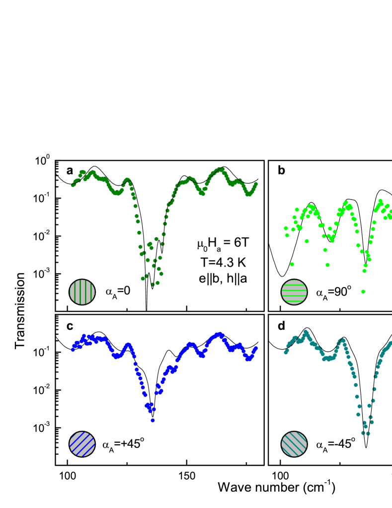
Figure 3: Optical activity in SmFe₃(BO₃)₄. Transmittance spectra for various mutual orientation of the polarizer and analyzer. a - Parallel geometry. b - Crossed geometry. c,d - $\pm 45^{\circ}$ geometry. Symbols - experiment, solid line - model calculations.

In order to prove that the dynamic magnetoelectric susceptibility induces optical activity in SmFe₃(BO₃)₄, we investigated the polarization state of the transmitted radiation as shown in Fig.3a,b. In these experiments the incident beam is linearly polarized. The transmitted power is measured for the analyzer rotated by the angle 0^∘, $90^{\circ}$, and $\pm 45^{\circ}$. Without optical activity the signal within $90^{\circ}$ (Fig. 3a) would be zero and the $\pm 45^{\circ}$ spectra (Figs. 3c,d) would coincide, which evidently contradict the spectra in Fig. 3. The evaluation of the transmitted power at different analyzer angle allows to fully characterize the polarization state of the transmitted radiation without additional measurements of the phase information. For example, the rotation angle $\theta$ and the ellipticity $\eta$ are given by

$$\tan(2\theta)=\frac{T(+45^{\circ})-T(-45^{\circ})}{T(0^{\circ})-T(90^{\circ})}\ ,\ \sin(2\eta)=\frac{\sqrt{4T(0^{\circ})T(90^{\circ})-[T(+45^{\circ})-T(-45^{\circ})]^{2}}}{T(0^{\circ})+T(90^{\circ})}\ ,$$ (3)

where $T(+45^{\circ}),T(-45^{\circ}),T(0^{\circ})$, and $T(90^{\circ})$ are the power transmission values for analyzer angle rotated by $+45^{\circ},-45^{\circ},0^{\circ}$, and $90^{\circ}$, respectively. This equation follows directly from Eq. 10.

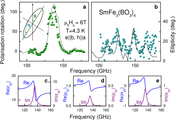
Figure 4: Polarization rotation by electromagnon in SmFe₃(BO₃)₄. a - Polarization rotation ($\theta$). The inset shows the definition of rotation angle and ellipticity. b - Ellipticity ($\eta$). c-e - electric, magnetic, and magnetoelectric permittivities as obtained from the model analysis of the transmission spectra at $\mu_{0}H=6$ T. Symbols - experiment, solid line - model calculations.

The angle of the polarization rotation and the ellipticity are shown in Fig. 4a,b. It is a remarkable result of these experiments that a polarization rotation angle exceeding 120 degrees is obtained for a sample with thickness of 1.7 millimeter only. We stress that this rotation arises purely from dynamic magnetoelectric susceptibility which is intrinsic for electromagnon in SmFe₃(BO₃)₄. Static magnetic field is in this case needed solely to lift the resonance frequency of the electromagnon into the available range of our spectrometer. This is in contrast to the polarization rotation by charge carriers palik_rpp_1970 or magnetic resonance zvezdin_book which require the Faraday geometry of the experiment and arise because of the off-diagonal elements in electric conductivity and magnetic permeability, respectively.

V Conclusions

In conclusion, this work demonstrates experimentally that the giant magnetodielectric effect in multiferroic ferroborate SmFe₃(BO₃)₄  arises as a result of a large electromagnon in the gigahertz frequency range. Based on symmetry arguments, the electromagnon in SmFe₃(BO₃)₄  reveals strong electric and magnetoelectric activity and can be controlled by external magnetic field. A polarization rotation exceeding 120 degrees is observed at gigahertz frequencies and is explained using dynamic magnetoelectric susceptibility in SmFe₃(BO₃)₄. Such a strong effect allows effective control of the gigahertz radiation via magnetoelectric effect.

Acknowledgements

This work was supported by Russian Foundation for Basic Researches (N 12-02-01261, 12-02-31461 mol), and by the Austrian Science Funds (I815-N16, W1243).

Appendix A Theory of dynamic magnetoelectric effect in S$\rm{m}$F$\rm{e}_{3}$(BO₃)₄

In order to describe the dynamic magnetic, magnetoelectric and magnetodielectric properties of SmFe₃(BO₃)₄ we shall consider the thermodynamical potential which depends on the ferromagnetic ($\mathbf{m}$) and antiferromagnetic ($\mathbf{l}$) vectors of the antiferromagnetically ordered Fe-subsystem, electric polarization $\mathbf{P}$ and external magnetic $\mathbf{H}$ and electric $\mathbf{E}$ fields:

$$\Phi(\mathbf{m},\mathbf{l},\mathbf{P},\mathbf{H},\mathbf{E})=\Phi_{m}(\mathbf{m},\mathbf{l},\mathbf{H})+\Phi_{me}(\mathbf{m},\mathbf{l},\mathbf{P})+\Phi_{e}(\mathbf{P},\mathbf{E})\ .$$ (4)

The first term in Eq. (4) represents the magnetic part in the antiferromagnetically ordered state with $l\gg m$ and $\mathbf{l}\bot\mathbf{m}$, and it is given by

$$\Phi_{m}(\mathbf{m},\mathbf{l},\mathbf{H})=\frac{1}{2}A\mathbf{m}^{2}-M_{0}\mathbf{m}\mathbf{H}+\Phi_{A}(\mathbf{l}),$$ (5)

where the first and second terms are the exchange and Zeeman energy, and the third term is the anisotropy energy

$$\Phi_{A}(\mathbf{l})=\frac{1}{2}K_{eff}l_{z}^{2}+\frac{1}{12}K_{6}\left[(l_{x}+il_{y})^{2}+(l_{x}-il_{y})^{2}\right]-\frac{1}{2}K_{1u}\left(l_{x}^{2}-l_{y}^{2}\right)-K_{2u}l_{x}l_{y}\ .$$

The uniaxial anisotropy stabilizes the magnetic moments within the basis $ab$ plane ($K_{eff}>0$) in which the anisotropy is determined by the hexagonal crystallographic anisotropy ($K_{6}$) and magnetoelastic anisotropy $K_{1u}\sim\sigma_{xx}-\sigma_{yy}$, $K_{2u}\sim\sigma_{xy}$ induced by internal stress (compression/elongation $\sigma_{xx}-\sigma_{yy}$ and shift $\sigma_{xy}$) in the crystallographic $ab$ plane.

In Eq. (4) the magnetoelectric energy $\Phi_{me}(\mathbf{m},\mathbf{l},\mathbf{P})$ relevant for the present analysis and related to the orientation of the Fe³⁺ spins in the basis $ab$ plane can be written as zvezdin_jetpl_2005 ; popov_prb_2013 :

$$\Phi_{me}(\mathbf{m},\mathbf{l},\mathbf{P})=-c_{2}P_{x}\left(l_{x}^{2}-l_{y}^{2}\right)+2c_{2}P_{y}l_{x}l_{y}+\mathellipsis\ .$$ (6)

The electric part $\Phi_{e}(\mathbf{P},\mathbf{E})$ of the thermodynamical potential Eq. (4) is determined by the expression

$$\Phi_{e}(\mathbf{P},\mathbf{E})=\left(P_{x}^{2}+P_{y}^{2}\right)/\left(2\chi_{\perp}^{e}\right)+P_{z}^{2}/\left(2\chi_{\|}^{e}\right)-\mathbf{P}\mathbf{E},$$ (7)

where $\chi_{\|}^{e}$ and $\chi_{\perp}^{e}$ are the crystal lattice parts of (di)electric susceptibility along and perpendicular to the $c$-axis, respectively. For the sake of simplicity the contribution of the Sm subsystem is not explicitly shown in Eqs. (4)-(6) but it is assumed that the corresponding parameters ($A$, $M_{0}$, $K_{eff}$, $c_{2}$, $\mathellipsis$) are renormalized due to Sm-Fe exchange interaction zvezdin_jetpl_2005 ; popov_prb_2013 .

By minimizing the thermodynamic potential $\Phi$ in Eq. (4) in $\mathbf{P}$ one obtains the equilibrium positions of the electric polarization:

$$P_{x}=P_{0}\left(l_{x}^{2}-l_{y}^{2}\right)+\chi_{\perp}^{e}E_{x},\quad P_{y}=-2P_{0}l_{x}l_{y}+\chi_{\perp}^{e}E_{y},\quad P_{z}=\chi_{\|}^{e}E_{z},$$

where $P_{0}=c_{2}\chi_{\perp}^{e}$ determines the maximal spontaneous polarization in the basis plane in a single-domain state, which is induced by the antiferromagnetic Fe ordering. Substituting $\mathbf{P}$ into Eq. (4) one can obtain the Landau–Lifshits equations for the dynamic magnetic variables $\mathbf{m}$ and $\mathbf{l}$:

$$\left(M_{0}/\gamma_{Fe}\right)\dot{\mathbf{m}}=\mathbf{m}\times\mathbf{\Phi}_{m}+\mathbf{l}\times\mathbf{\Phi}_{l},\quad\left(M_{0}/\gamma_{Fe}\right)\dot{\mathbf{l}}=\mathbf{m}\times\mathbf{\Phi}_{l}+\mathbf{l}\times\mathbf{\Phi}_{m},$$ (8)

where $\mathbf{\Phi}_{m}=\partial\Phi/\partial\mathbf{m}$, $\mathbf{\Phi}_{l}=\partial\Phi/\partial\mathbf{l}$ and $\gamma_{Fe}=g_{Fe}\mu_{B}/\hbar$ is the gyromagnetic ratio for Fe-ions. The linearization and solution of these equations with respect to small oscillations of $\mathbf{m}$ and $\mathbf{l}$ in the easy plane state $\mathbf{l}_{0}\|\mathbf{b}$ stabilized by the magnetic field $\mathbf{H}\|\mathbf{a}$ allows to derive the magnetic and electric response to the alternating fields $\mathbf{e}$ and $\mathbf{h}$:

$$\begin{array}[]{c}\Delta\mathbf{m}=\chi^{m}\mathbf{h}+\chi^{me}\mathbf{e},\\ \Delta\mathbf{p}=\chi^{em}\mathbf{h}+\chi^{e}\mathbf{e}.\\ \end{array}$$

Here magnetic $\chi^{m}$, magnetoelectric $\chi^{me}$, $\chi^{em}$ and dielectric $\chi^{e}$ susceptibilities are given by

$$\begin{array}[]{cc}\hat{\chi}^{m}(\omega)=\left(\begin{array}[]{ccc}\chi_{xx}^{m}&0&0\\ 0&\chi_{yy}^{m}&\chi_{yz}^{m}\\ 0&\chi_{zy}^{m}&\chi_{zz}^{m}\\ \end{array}\right)&\hat{\chi}^{me}(\omega)=\left(\begin{array}[]{ccc}\chi_{xx}^{me}&0&0\\ 0&\chi_{yy}^{me}&0\\ 0&\chi_{zy}^{me}&0\\ \end{array}\right)\\[30.00005pt] \hat{\chi}^{em}(\omega)=\left(\begin{array}[]{ccc}\chi_{xx}^{em}&0&0\\ 0&\chi_{yy}^{em}&\chi_{yz}^{em}\\ 0&0&0\\ \end{array}\right)&\hat{\chi}^{e}(\omega)=\left(\begin{array}[]{ccc}\chi_{xx}^{e}&0&0\\ 0&\chi_{yy}^{e}&0\\ 0&0&\chi_{zz}^{e}\\ \end{array}\right).\\ \end{array}$$

where the individual terms are obtained as:

$$\chi_{xx}^{m} = \chi_{\perp}L_{AF}(\omega)$$

$$\chi_{zz}^{m} = \chi_{\perp}L_{F}(\omega)$$

$$\chi_{yy}^{m} = \rho^{2}\chi_{\perp}L_{F}(\omega)$$

$$\chi_{zy}^{m} = (-i\omega/\omega_{F})\sqrt{\chi_{yy}^{m}\chi_{zz}^{m}}=(-i\omega/\omega_{F})\rho\chi_{\perp}L_{F}(\omega)$$

$$\chi_{yy}^{e} = \chi_{\perp}^{e}+\chi_{rot}^{e}L_{F}(\omega)$$

$$\chi_{xx,zz}^{e} = \chi_{\perp,\|}^{e}$$

$$\chi_{xx}^{me} = \chi_{xx}^{em}\approx 0$$

$$\chi_{yy}^{me} = \chi_{yy}^{em}=\rho\eta\sqrt{\chi_{\perp}\chi_{rot}^{e}}L_{F}(\omega)$$

$$\chi_{zy}^{me} = -\chi_{yz}^{em}=(i\omega/\omega_{F})\eta\sqrt{\chi_{\perp}\chi_{rot}^{e}}L_{F}(\omega)$$

Here $\chi_{\perp}=M_{0}^{2}/A\equiv M_{0}/(2H_{E})$ is the transverse magnetic susceptibility, $M_{0}$ and $H_{E}$ are the magnetization of the saturated antiferromagnetic sublattices of Fe³⁺ ions and Fe-Fe exchange field, respectively. $\chi_{rot}^{e}$ is the electric susceptibility along the $b$-axis due to the rotation of the spins in the basis plane. The magnetic field dependence of $\chi_{rot}^{e}$ is given by

$$\chi_{rot}^{e}=\frac{\chi_{0rot}^{e}}{1+H^{2}/(2H_{A}^{\prime}H_{E})}$$

where $\chi_{0rot}^{e}=(2P_{0})^{2}/K_{A}^{\prime}$ is the value of $\chi_{rot}^{e}$ at $H=0$ and $K_{A}^{\prime}=\partial^{2}\Phi_{A}/\partial\varphi^{2}\left|{}_{\varphi=\pm\pi/2}\right.$ is the effective anisotropy energy in the basis plane for the orientation $\mathbf{l}\|\mathbf{b}$ $(\varphi=\pm\pi/2)$ kuzmenko_jetp_2011 (see also Ref. note1 ).

The functions

$$L_{F,AF}(\omega)=\omega_{F,AF}^{2}/\left(\omega_{F,AF}^{2}-\omega^{2}+i\omega\Delta\omega_{F,AF}\right)$$

determine the frequency dispersion of the electrodynamic response near the resonance frequencies of the quasi-ferromagnetic (in-plane) mode

$$\omega_{F}^{2}=\gamma^{2}\left(H^{2}+2H_{A}^{\prime}H_{E}\right)$$

and the quasi-antiferromagnetic (out-of-plane) mode

$$\omega_{AF}^{2}=2\gamma^{2}H_{A}H_{E}\ ,$$

where $H_{A}^{\prime}=K_{A}^{\prime}/M_{0}$ and $H_{A}=K_{A}/M_{0}$ are the corresponding anisotropy fields, $\Delta\omega_{F,AF}$ are the line-widths of the modes which are determined by dissipation terms omitted in Eq. (8).

The factor $\rho(H)=H/\sqrt{H^{2}+2H_{A}^{\prime}H_{E}}$ reflects the changes of the magnetic structure with increasing magnetic field and becomes unity in the fields exceeding 5-10 kOe, the factor $\eta=(V^{+}-V^{-})/(V^{+}+V^{-})$ takes into account possible existence of structural twins with opposite chirality with concentrations $V^{\pm}$ and with opposite contributions to the electric polarization.

The derivation of the magnetoelectric response given above has been performed assuming that the resonance frequencies of the rare-earth (Sm) ions determined by the exchange (R-Fe) splitting of its ground doublet are higher than the AFMR frequencies of Fe-subsystem. This condition is fully satisfied for the low frequency quasi-ferromagnetic mode $\omega_{F}$ where the giant magnetoelectric activity is observed. On the contrary, the frequency of quasi-antiferromagnetic mode $\omega_{AF}$ is comparable to that of the corresponding Sm-mode and, therefore, a coupling of Fe and Sm magnetic oscillation cannot be neglected kuzmenko_jetpl_2011 . However, due to high frequencies of these modes the dynamic magnetoelectric effect is weak and has not been observed.

Appendix B Data processing

The light propagating along the $z$ direction can be characterized by the tangential components of electric ($E_{x}$, $E_{y}$) and magnetic ($H_{x}$, $H_{y}$) fields. We write these components in the form of a 4D vector $\mathbf{V}$:

$$\mathbf{V}=\left(\begin{array}[]{c}E_{x}\\ E_{y}\\ H_{x}\\ H_{y}\\ \end{array}\right).$$

The interconnection between vectors $\mathbf{V}_{1}$ and $\mathbf{V}_{2}$, corresponding to different points in space separated by a distance $d$, is given by $\mathbf{V}_{1}=M(d)\mathbf{V}_{2}$. Here, $M(d)$ is a 4x4 transfer matrix. The susceptibility tensor for SmFe(BO₃)₄ has the form:

$$\left(\begin{array}[]{c}D_{x}\\ D_{y}\\ D_{z}\\ B_{x}\\ B_{y}\\ B_{z}\\ \end{array}\right)=\left(\begin{array}[]{cccccc}\varepsilon_{xx}&0&0&0&0&0\\ 0&\varepsilon_{yy}&0&0&\alpha_{yy}&\alpha_{yz}\\ 0&0&\varepsilon_{zz}&0&0&0\\ 0&0&0&\mu_{xx}&0&0\\ 0&\alpha_{yy}&0&0&\mu_{yy}&\mu_{yz}\\ 0&-\alpha_{yz}&0&0&\mu_{zy}&\mu_{zz}\\ \end{array}\right)\left(\begin{array}[]{c}E_{x}\\ E_{y}\\ E_{z}\\ H_{x}\\ H_{y}\\ H_{z}\\ \end{array}\right).$$ (9)

The total transfer matrix $M$ is calculated following Berreman’s method berreman_josa_1972 . In the case of normal incidence the electromagnetic field inside the sample has the form of a plane wave $\exp(i(k_{z}z-\omega t))$. The value of $k_{z}$ depends on the properties of the sample and is determined solving the Maxwell equations within the sample. In a first step the normal field components $E_{z}$ and $H_{z}$ are expressed in terms of four tangential components using Maxwell’s equations together with the constitutive relations Eq. (9) above. The remaining four equations in four variables $E_{x},E_{y},H_{x},H_{y}$ can be represented in the form of an eigenvalue problem with 4x4 matrix. The eigenvalues give four possible values of $k_{z}$ and correspond to four waves propagating inside the sample: two polarizations in positive $z$ direction and two polarizations in the negative direction. The polarizations of these waves are given by the corresponding eigenvectors of the solution. The choice of the tangential field components simplify the calculations because $E_{x},E_{y},H_{x},H_{y}$ are continuous at the sample-air boundary. The described procedure is only slightly modified in the case of oblique incidence.

As a next step, the transfer matrix $M(d)$, which relates vectors $\mathbf{V}$ in the air (vacuum) on both sides of the sample, is written as

$$M(d)=WK(d)W^{-1}\ .$$

The matrix $W$ is composed of four eigenvectors of the solution above and it transfers the tangential field components into the waves which propagate inside the sample. The diagonal matrix $K_{jj}=\exp(ik_{z}^{(j)}d)$ is constructed out of four eigenvalues $k_{z}^{(j)}$, $j=1,\ldots,4$ and it describes the propagation of the electromagnetic eigenmodes along the $z$-direction.

To illustrate the procedure with a simple example, we describe an isotropic dielectric medium with simple constitutive equations $\mathbf{D}=\varepsilon\mathbf{E}$ and $\mathbf{B}=\mu\mathbf{H}$. In the case of normal incidence the eigenvalue problem can be written as:

$$\frac{ck_{z}}{\omega}\mathbf{V}=\left(\begin{array}[]{cccc}0&0&0&\mu\\ 0&0&-\mu&0\\ 0&-\varepsilon&0&0\\ \varepsilon&0&0&0\\ \end{array}\right)\mathbf{V}.$$

The matrices $W$ and $K(d)$ are given by:

$$W=\left(\begin{array}[]{cccc}Z&Z&0&0\\ 0&0&Z&Z\\ 0&0&-1&1\\ 1&-1&0&0\\ \end{array}\right),\quad K(d)=\left(\begin{array}[]{cccc}e^{ikd}&0&0&0\\ 0&e^{-ikd}&0&0\\ 0&0&e^{ikd}&0\\ 0&0&0&e^{-ikd}\\ \end{array}\right).$$

Here, $Z=\sqrt{\mu/\varepsilon}$ and $k=\sqrt{\mu\varepsilon}\,\omega/c$. The resulting transfer matrix $M(d)=WK(d)W^{-1}$ takes the form:

$$M(d)=\left(\begin{array}[]{cccc}\cos(kd)&0&0&iZ\sin(kd)\\ 0&\cos(kd)&-iZ\sin(kd)&0\\ 0&-iZ^{-1}\sin(kd)&\cos(kd)&0\\ iZ^{-1}\sin(kd)&0&0&\cos(kd)\\ \end{array}\right).$$

In order to calculate the complex transmission and reflection coefficients it is more convenient to change the basis. In the new basis, the first component of the vector $\mathbf{V}$ is the amplitude of the linearly polarized wave ($E_{x}$) propagating in positive direction, the second - of the wave with the same polarization propagating in negative direction and the third and the fourth components - of two waves with another linear polarization ($E_{y}$). The propagation matrix in the new basis is $M^{\prime}=V^{-1}MV$, with the transformation matrix given by:

$$V=\left(\begin{array}[]{cccc}1&1&0&0\\ 0&0&1&1\\ 0&0&-1&1\\ 1&-1&0&0\\ \end{array}\right).$$

The complex transmission and reflection coefficients for the linearly polarized incident radiation can now be found from the following system of equations:

$$\left(\begin{array}[]{c}t_{\perp}\\ 0\\ t_{\|}\\ 0\\ \end{array}\right)=M^{\prime}\left(\begin{array}[]{c}0\\ r_{\perp}\\ 1\\ r_{\|}\\ \end{array}\right).$$

Here the $t_{\|}$ and $t_{\perp}$ denote the complex transmittance amplitudes within parallel and crossed polarizers, respectively; the same conventions for reflectance are given by $r_{\|}$ and $r_{\perp}$. In the simple example above the transfer matrix contains four relevant elements only:

$$M^{\prime}=\left(\begin{array}[]{cccc}c_{d}+i\frac{Z+Z^{-1}}{2}s_{d}&i\frac{Z^{-1}-Z}{2}s_{d}&0&0\\ i\frac{Z-Z^{-1}}{2}s_{d}&c_{d}-i\frac{Z+Z^{-1}}{2}s_{d}&0&0\\ 0&0&c_{d}+i\frac{Z+Z^{-1}}{2}s_{d}&i\frac{Z^{-1}-Z}{2}s_{d}\\ 0&0&i\frac{Z-Z^{-1}}{2}s_{d}&c_{d}-i\frac{Z+Z^{-1}}{2}s_{d}\\ \end{array}\right),$$

where $c_{d}=\cos(kd)$ and $s_{d}=\sin(kd)$. The complex transmission coefficient in this case is well known and can be written explicitly as:

$$t_{\|}=\left(\cos(kd)-i\frac{Z+Z^{-1}}{2}\sin(kd)\right)^{-1}\ .$$

In particular case when the measurements are performed with the analyzer rotated by $\pm 45^{\circ}$ to the incident radiation, the corresponding complex transmission coefficients $t_{\pm 45}$ are related to transmission in parallel $t_{\|}$ and crossed $t_{\perp}$ geometries as:

$$\left(\begin{array}[]{c}t_{+45}\\ t_{-45}\\ \end{array}\right)=\frac{1}{\sqrt{2}}\left(\begin{array}[]{cc}1&1\\ 1&-1\\ \end{array}\right)\left(\begin{array}[]{c}t_{\|}\\ t_{\perp}\\ \end{array}\right).$$ (10)

The polarization rotation $\theta$ and the ellipticity $\eta$ are obtained from the transmission data using palik_rpp_1970 :

$$\tan(2\theta)=2\Re(\chi)/(1-|\chi|^{2})\ ,$$

$$\sin(2\eta)=2\Im(\chi)/(1+|\chi|^{2})\ .$$

Here $\chi=t_{\perp}/t_{\|}$ and the definitions of $\theta+i\eta$ are shown schematically in Fig. 4a.

References

- [1] M. Fiebig. Revival of the magnetoelectric effect. J. Phys. D: Appl. Phys., 38(8):R123, 2005.
- [2] R. Ramesh and N. A. Spaldin. Multiferroics: progress and prospects in thin films. Nat. Mater., 6(1):21, Jan 2007.
- [3] W. Eerenstein, N. D. Mathur, and J. F. Scott. Multiferroic and magnetoelectric materials. Nature, 442(7104):759, Aug 2006.
- [4] Yoshinori Tokura. Multiferroics as quantum electromagnets. Science, 312(5779):1481, 2006.
- [5] A. N. Vasiliev and E. A. Popova. Rare-earth ferroborates RFe3(BO3)4. Low Temp. Phys., 32(8):735–747, 2006.
- [6] A. M. Kadomtseva, Yu. F. Popov, G. P. Vorob’ev, A. P. Pyatakov, S. S. Krotov, K. I. Kamilov, V. Yu. Ivanov, A. A. Mukhin, A. K. Zvezdin, A. M. Kuz’menko, L. N. Bezmaternykh, I. A. Gudim, and V. L. Temerov. Magnetoelectric and magnetoelastic properties of rare-earth ferroborates. Low Temperature Physics, 36(6):511–521, 2010.
- [7] K.-C. Liang, R. P. Chaudhury, B. Lorenz, Y. Y. Sun, L. N. Bezmaternykh, V. L. Temerov, and C. W. Chu. Giant magnetoelectric effect in HoAl3(BO3)4. Phys. Rev. B, 83:180417, May 2011.
- [8] A. A. Mukhin, G. P. Vorob’ev, V. Yu. Ivanov, A. M. Kadomtseva, A. S. Narizhnaya, A. M. Kuz’menko, Yu. F. Popov, L. N. Bezmaternykh, and I. A. Gudim. Colossal magnetodielectric effect in SmFe3(BO3)4 multiferroic. JETP Lett., 93(5):275–281, 2011.
- [9] R. P. Chaudhury, F. Yen, B. Lorenz, Y. Y. Sun, L. N. Bezmaternykh, V. L. Temerov, and C. W. Chu. Magnetoelectric effect and spontaneous polarization in HoFe3(BO3)4 and Ho0.5Nd0.5Fe3(BO3)4. Phys. Rev. B, 80:104424, Sep 2009.
- [10] F. Kagawa, M. Mochizuki, Y. Onose, H. Murakawa, Y. Kaneko, N. Furukawa, and Y. Tokura. Dynamics of multiferroic domain wall in spin-cycloidal ferroelectric DyMnO3. Phys. Rev. Lett., 102(5):057604, Feb 2009.
- [11] P. Lunkenheimer, V. Bobnar, A. V. Pronin, A. I. Ritus, A. A. Volkov, and A. Loidl. Origin of apparent colossal dielectric constants. Phys. Rev. B, 66:052105, Aug 2002.
- [12] A.M. Kuz’menko, A.A. Mukhin, V.Yu. Ivanov, A.M. Kadomtseva, S.P. Lebedev, and L.N. Bezmaternykh. Antiferromagnetic resonance and dielectric properties of rare-earth ferroborates in the submillimeter frequency range. J. Exp. Theor. Phys., 113(1):113–120, 2011.
- [13] A. Pimenov, A. M. Shuvaev, A. A. Mukhin, and A. Loidl. Electromagnons in multiferroic manganites. J. Phys.: Condens. Matter, 20(43):434209, 2008.
- [14] A. B. Sushkov, M. Mostovoy, R. Valdes Aguilar, S.-W. Cheong, and H. D. Drew. Electromagnons in multiferroic RMn2O5 compounds and their microscopic origin. J. Phys.: Condens. Matter, 20(43):434210, 2008.
- [15] A. Pimenov, A. A. Mukhin, V. Yu. Ivanov, V. D. Travkin, A. M. Balbashov, and A. Loidl. Possible evidence for electromagnons in multiferroic manganites. Nat. Phys., 2(2):97, Feb 2006.
- [16] N. Kida, S. Kumakura, S. Ishiwata, Y. Taguchi, and Y. Tokura. Gigantic terahertz magnetochromism via electromagnons in the hexaferrite magnet Ba2Mg2Fe12O22. Phys. Rev. B, 83:064422, Feb 2011.
- [17] S. Bordacs, I. Kezsmarki, D. Szaller, L. Demko, N. Kida, H. Murakawa, Y. Onose, R. Shimano, T. Room, U. Nagel, S. Miyahara, N. Furukawa, and Y. Tokura. Chirality of matter shows up via spin excitations. Nat. Phys., 8(10):734–738, Oct 2012.
- [18] I. Kézsmárki, N. Kida, H. Murakawa, S. Bordács, Y. Onose, and Y. Tokura. Enhanced directional dichroism of terahertz light in resonance with magnetic excitations of the multiferroic Ba2CoGe2O7 oxide compound. Phys. Rev. Lett., 106:057403, Feb 2011.
- [19] Youtarou Takahashi, Ryo Shimano, Yoshio Kaneko, Hiroshi Murakawa, and Yoshinori Tokura. Magnetoelectric resonance with electromagnons in a perovskite helimagnet. Nat. Phys., 8(2):121–125, Feb 2012.
- [20] Y. Takahashi, Y. Yamasaki, and Y. Tokura. Terahertz magnetoelectric resonance enhanced by mutual coupling of electromagnons. Phys. Rev. Lett., 111:037204, Jul 2013.
- [21] A. Shuvaev, V. Dziom, Anna Pimenov, M. Schiebl, A. A. Mukhin, A. C. Komarek, T. Finger, M. Braden, and A. Pimenov. Electric field control of terahertz polarization in a multiferroic manganite with electromagnons. Phys. Rev. Lett., 111:227201, Nov 2013.
- [22] P. Rovillain, R. de Sousa, Y. Gallais, A. Sacuto, M. A. Measson, D. Colson, A. Forget, M. Bibes, A. Barthelemy, and M. Cazayous. Electric-field control of spin waves at room temperature in multiferroic BiFeO3. Nat. Mater., 9(12):975–979, Dec 2010.
- [23] A. K. Zvezdin, G. P. Vorob’ev, A. M. Kadomtseva, Yu. F. Popov, A. P. Pyatakov, L. N. Bezmaternykh, A. V. Kuvardin, and E. A. Popova. Magnetoelectric and magnetoelastic interactions in NdFe3(BO3)4 multiferroics. JETP Lett., 83(11):509–514, 2006.
- [24] H. Katsura, A. V. Balatsky, and N. Nagaosa. Dynamical magnetoelectric coupling in helical magnets. Phys. Rev. Lett., 98(2):027203, 2007.
- [25] M. Mostovoy. Ferroelectricity in spiral magnets. Phys. Rev. Lett., 96(6):067601, 2006.
- [26] R. Valdes Aguilar, M. Mostovoy, A. B. Sushkov, C. L. Zhang, Y. J. Choi, S-W. Cheong, and H. D. Drew. Origin of electromagnon excitations in multiferroic RMnO3. Phys. Rev. Lett., 102(4):047203, 2009.
- [27] J. S. Lee, N. Kida, S. Miyahara, Y. Takahashi, Y. Yamasaki, R. Shimano, N. Furukawa, and Y. Tokura. Systematics of electromagnons in the spiral spin-ordered states of RMnO3. Phys. Rev. B, 79(18):180403, 2009.
- [28] A. A. Volkov, Yu. G. Goncharov, G. V. Kozlov, S. P. Lebedev, and A. M. Prokhorov. Dielectric measurements in the submillimeter wavelength region. Infrared Phys., 25(1-2):369, 1985.
- [29] A. M. Shuvaev, G. V. Astakhov, C. Brüne, H. Buhmann, L. W. Molenkamp, and A. Pimenov. Terahertz magneto-optical spectroscopy in HgTe thin films. Semicond. Sci. Technol., 27(12):124004, 2012.
- [30] D. W. Berreman. Optics in stratified and anisotropic media - 4x4-matrix formulation. J. Opt. Soc. Am., 62(4):502, 1972.
- [31] A. K. Zvezdin, S. S. Krotov, A. M. Kadomtseva, G. P. Vorob’ev, Yu. F. Popov, A. P. Pyatakov, L. N. Bezmaternykh, and E. A. Popova. Magnetoelectric effects in gadolinium iron borate GdFe3(BO3)4. JETP Lett., 81(6):272–276, 2005.
- [32] A. I. Popov, D. I. Plokhov, and A. K. Zvezdin. Quantum theory of magnetoelectricity in rare-earth multiferroics: Nd, Sm, and Eu ferroborates. Phys. Rev. B, 87:024413, Jan 2013.
- [33] E. D. Palik and J. K. Furdyna. Infrared and microwave magnetoplasma effects in semiconductors. Rep. Prog. Phys., 33(3):1193, 1970.
- [34] A. K. Zvezdin and V. A. Kotov. Modern Magnetooptics and Magnetooptical Materials. Condensed Matter Physics. Taylor & Francis, 2010.
- [35] The value of the in-plane anisotropy can be either positive or negative depending on the interrelation between the hexagonal crystallographic anisotropy and the magnetoelastic anisotropy induced by internal stress. Moreover, its effective value and the easy axis direction in the basis plane can be distributed due to inhomogeneous internal stress. In this case the corresponding rotational electric susceptibility should be determined by averaging over a whole crystal. However, in magnetic fields exceeding the in-plane spin-flop field 5-10 kOe when spins are aligned perpendicular to an external magnetic field, the behavior of the rotational electric susceptibility is determined basically by the field-induced anisotropy in the basis plane .
- [36] A.M. Kuz’menko, A.A. Mukhin, V.Yu. Ivanov, A.M. Kadomtseva, and L.N. Bezmaternykh. Effects of the interaction between R and Fe modes of the magnetic resonance in RFe3(BO3)4 rare-earth iron borates. JETP Lett., 94(4):294–300, 2011.