Langevin dynamics for ramified structures

Abstract

We propose a generalized Langevin formalism to describe transport in combs and similar ramified structures. Our approach consists of a Langevin equation without drift for the motion along the backbone. The motion along the secondary branches may be described either by a Langevin equation or by other types of random processes. The mean square displacement (MSD) along the backbone characterizes the transport through the ramified structure. We derive a general analytical expression for this observable in terms of the probability distribution function of the motion along the secondary branches. We apply our result to various types of motion along the secondary branches of finite or infinite length, such as subdiffusion, superdiffusion, and Langevin dynamics with colored Gaussian noise and with non-Gaussian white noise. Monte Carlo simulations show excellent agreement with the analytical results. The MSD for the case of Gaussian noise is shown to be independent of the noise color. We conclude by generalizing our analytical expression for the MSD to the case where each secondary branch is $n$ dimensional.

I Introduction

Various phenomena in physics, biology, geology, and other fields involve the transport or motion of particles, microorganisms, and fluids in ramified structures. Examples range from fluid flow through porous media to oil recovery, respiration, and blood circulation. Ramified structures like river networks Rodríguez-Iturbe and Rinaldo (1997) represent examples of ecological corridors, which have significant implications in epidemics Bertuzzo et al. (2010) or diversity patterns Muneepeerakul et al. (2008), among other. Ramified structures have also attracted the attention of physicists because the transport of particles across them displays anomalous diffusion Forte et al. (2013).

The simplest models of these various types of natural structures, which belong to the category of loopless graphs, are the comb model and the Peano network, two ramified structures that have been applied, for example, to explain biological invasion through river networks Méndez et al. (2010). Comb structures consist of a principal branch, the backbone, which is a one-dimensional lattice with spacing $a$, and identical secondary branches, the teeth, that cross the backbone perpendicularly. We identify the direction of the backbone with the $x$-axis, while the secondary branches lie parallel to the $y$-axis. Nodes on the backbone have the coordinates $(ia,0)$, with $i=0,\pm 1,\pm 2,\dotsc$, while nodes on the teeth have coordinates $(ia,ja)$, with $j=0,\pm 1,\pm 2,\dotsc$ and $i$ fixed.

The comb model was originally introduced to understand anomalous diffusion in percolating clusters Weiss and Havlin (1986); White and Barma (1984); Arkhincheev and Baskin (1991). If particles undergo a simple random walk on the comb structure, the secondary branches act like traps in which the particle stays for some random time before continuing its random motion along the backbone. This results in a mean square displacement (MSD) $\left\langle x^{2}(t)\right\rangle\sim\sqrt{t}$, i.e., subdiffusive behavior along the backbone. Nowadays, comb-like models are widely used to describe different experimental applications, such as anomalous transport along spiny dendrites Méndez and Iomin (2013); Iomin and Méndez (2013); Fedotov and Méndez (2008) and dendritic polymers Frauenrath (2005), to mention just a few.

In the continuum limit, transport on a comb can be described by an anisotropic diffusion equation,

$$\frac{\partial P(x,y,t)}{\partial t}=[C(y)]^{2}D_{x}\frac{\partial^{2}P(x,y,t)}{\partial x^{2}}+D_{y}\frac{\partial^{2}P(x,y,t)}{\partial y^{2}}.$$ (1)

This diffusion equation is equivalent to the system of Langevin equations

$$\frac{dX}{dt} =C(Y)\xi_{x}(t),$$ (2a)

$$\frac{dY}{dt} =\xi_{y}(t),$$ (2b)

where $\xi_{x}(t)$ and $\xi_{y}(t)$ are two uncorrelated Gaussian white noises with

$$\left\langle\xi_{x}(t)\right\rangle =\left\langle\xi_{y}(t)\right\rangle=0,$$ (3a)

$$\left\langle\xi_{x}(t)\xi_{x}(t^{\prime})\right\rangle =2D_{x}\delta(t-t^{\prime}),$$ (3b)

$$\left\langle\xi_{y}(t)\xi_{y}(t^{\prime})\right\rangle =2D_{y}\delta(t-t^{\prime}),$$ (3c)

$$\left\langle\xi_{x}(t)\xi_{y}(t^{\prime})\right\rangle =0.$$ (3d)

Here $\langle\cdot\rangle$ denotes averaging over the noises. Eq. (1) can be obtained assuming both Ito and Stratonovich interpretations since the specific form of the Langevin equations (2) yields to the same Wong-Zakai terms.

The coefficient $C(y)$ in Eq. (1) introduces a heterogeneity that couples the motion in both directions. In most works about transport on combs Arkhincheev and Baskin (1991); Arkhincheev (1999); Baskin and Iomin (2004) this coefficient is taken to be $\left[C(y)\right]^{2}=\delta(y)$, a Dirac delta function, which means that the teeth cross the backbone only at $y=0$. The system of equations (2) has also been applied to certain problems in biochemical kinetics Bel and Nemenman (2009); Ribeiro et al. (2014).

Our goal is to apply the Langevin equations (2) to situations where the motion of particles does not correspond to simple Brownian motion. In particular we will focus on the case where the driving noises along the teeth, i.e., in the $y$-direction are no longer Gaussian white noises. In other words, we consider combs where the transport process along the teeth can differ fundamentally from the transport process along the backbone

The paper is organized as follows. In Sec. II we introduce our generalized Langevin description. An exact analytical expression for the MSD along the backbone is derived in Sec. III. We use that result to investigate the effect of subdiffusive and superdiffusive motion along the teeth, motion driven by various types of noises, as well as the effect of the geometry of the teeth in Secs. IV, V, and VI. We discuss our results in Sec. VII.

II Langevin Equations

Consider first a ramified structure where the particle dynamics is governed by the general Langevin equations

$$\frac{dX}{dt} =\beta_{x}C(Y)\xi_{x}(t),$$ (4a)

$$\frac{dY}{dt} =\xi_{y}(t).$$ (4b)

Here $(X(t),Y(t))$ is a random process describing the position of the particle in a two-dimensional space, and $\beta_{x}$ is a positive parameter. The random driving forces $\xi_{x}$ and $\xi_{y}$ are two external noises that drive the motion of the particle along the $x$-direction, backbone or main direction, and the $y$-direction, branches or secondary direction, respectively. The motion along the $y$-direction is then independent of the $x$ coordinate. The coupling of the motions along the $x$ and $y$ directions is described by $C(Y)$. In fact, we will consider a more general system than Eqs. (4). The random process $Y(t)$ does not have to be given by the Langevin equation (4b); it can be any suitable random process describing the motion in the $y$-direction, as long as it is independent of $X(t)$. In the following, $\left\langle\cdot\right\rangle$ denotes averaging over one random variable, e.g. $X$, and $\left\langle\left\langle\cdot\right\rangle\right\rangle$ over all random variables involved, e.g., $X$ and $Y$. To determine the MSD we rewrite Eq. (4a) in the form

$$\frac{d}{dt}(X^{2})=2\beta_{x}C[Y(t)]\xi_{x}(t)X(t).$$ (5)

We integrate Eq. (4a) with the initial condition $X(0)=0$, substitute the result into Eq. (5), and average over the noise $\xi_{x}(t)$ to find

$$\frac{d}{dt}\left\langle X^{2}(t)\right\rangle=2\beta_{x}^{2}C[Y(t)]\int_{0}^{t}C[Y(t^{\prime})]\left\langle\xi_{x}(t)\xi_{x}(t^{\prime})\right\rangle dt^{\prime}.$$ (6)

In the following we assume in all cases that the noise $\xi_{x}(t)$ driving the motion along the backbone is white, i.e., $\left\langle\xi_{x}(t)\xi_{x}(t^{\prime})\right\rangle=2D_{x}\delta(t-t^{\prime})$, and we adopt the Stratonovich interpretation. We also consider for simplicity that both noises $\xi_{x}$ and $\xi_{y}$ are uncorrelated. Then Eq. (6) turns into

$$\frac{d}{dt}\left\langle X^{2}(t)\right\rangle=2D_{x}\beta_{x}^{2}\left(C[Y(t)]\right)^{2}.$$ (7)

Let $\mathcal{D}$ be the range of $Y(t)$. Then averaging Eq. (7) over $Y$, we obtain

$$\frac{d}{dt}\left\langle\left\langle X^{2}(t)\right\rangle\right\rangle=2D_{x}\beta_{x}^{2}\int_{\mathcal{D}}(C[y])^{2}P_{Y}(y,t)dy,$$ (8)

where $P_{Y}(y,t)=\langle\delta(Y(t)-y)\rangle$. Consequently, the MSD for transport through the ramified structure is given by

$$\left\langle\left\langle X^{2}(t)\right\rangle\right\rangle=2D_{x}\beta_{x}^{2}\int_{0}^{t}dt^{\prime}\int_{\mathcal{D}}(C[y])^{2}P_{Y}(y,t^{\prime})dy.$$ (9)

III The Mean Square Displacement

We use the result (9) to assess the influence of various types of motion in the $y$-direction on the transport through the structure. The simplest case occurs if the structure is actually not ramified at all, i.e., the particles move in the $x$-$y$-plane. The dynamics of $X(t)$ and $Y(t)$ are independent, i.e., $C[Y(t)]=C=$ const. We obtain from Eq. (9)

$$\left\langle\left\langle X^{2}(t)\right\rangle\right\rangle=2D_{x}\beta_{x}^{2}C^{2}t.$$ (10)

In other words, the motion projected into the $x$-axis corresponds to normal diffusive behavior. This is the expected result, since $X(t)$ does not depend on $Y(t)$ and is driven by white noise.

More interesting behavior occurs for a comb-like structure. To account for this case we consider that the coupling function can be written as

$$C[y]=\sqrt{\frac{\ell}{\pi(y^{2}+\ell^{2})}}.$$ (11)

Note that $C^{2}[y]$ is a regularization, or representation, of the Dirac delta function for $\ell\rightarrow 0$. So, invoking the fact that $C^{2}[y]\rightarrow\delta(y)$ for $\ell\rightarrow 0$, Eq. (9) reads

$$\left\langle\left\langle X^{2}(t)\right\rangle\right\rangle =2\beta_{x}^{2}D_{x}\int_{0}^{t}dt^{\prime}\int_{-\infty}^{\infty}P_{Y}(y,t^{\prime})\delta(y)dy$$

$$=2\beta_{x}^{2}D_{x}\int_{0}^{t}dt^{\prime}P_{Y}(y=0,t^{\prime})$$ (12)

or in Laplace space

$$\left\langle\left\langle\hat{X}^{2}(s)\right\rangle\right\rangle=2\beta_{x}^{2}D_{x}\frac{\hat{P}_{Y}(y=0,s)}{s},$$ (13)

where the hat symbol denotes the Laplace transform and $s$ is the Laplace variable.

Taking into account the inverse Fourier transform $P_{Y}(y,t)=(1/2\pi)\int_{-\infty}^{\infty}dk\exp(-iky)P_{Y}(k,t)$, it is easy to see that $\hat{P}_{Y}(y=0,s)=(1/2\pi)\int_{-\infty}^{\infty}dk\hat{P}_{Y}(k,s)$. Substituting this result into (13), we find that the MSD reads

$$\left\langle\left\langle\hat{X}^{2}(s)\right\rangle\right\rangle=\frac{\beta_{x}^{2}D_{x}}{\pi s}\int_{-\infty}^{\infty}dk\hat{P}_{Y}(k,s),$$ (14)

i.e., we can determine the MSD in Laplace space if we know the propagator, in Fourier-Laplace space, along the teeth.

IV Secondary branches with infinite length

Note that our results for the MSD, Eqs. (12) – (14), are valid as long as the movement along the backbone follows the Langevin dynamics given by Eq. (4a). The motion of the particles along the teeth need not be governed by the Langevin dynamics Eq. (4b); it can be any suitable random process. In this Section we explore transport through the comb when the movement of particles along the teeth is anomalous, i.e., non-standard diffusion.

IV.1 Continuous-Time Random Walk

We consider here the case where the motion along the teeth can be described by a Continuous-Time Random Walk (CTRW). The propagator in Fourier-Laplace space $\hat{P}_{Y}(k,s)$ is given, in general, by the Montroll-Weiss equation Montroll and Weiss (1965), and we obtain from Eq. (14)

$$\left\langle\left\langle\hat{X}^{2}(s)\right\rangle\right\rangle=\frac{\beta_{x}^{2}D_{x}[1-\hat{\phi}(s)]}{\pi s^{2}}\int_{-\infty}^{\infty}\frac{dk}{1-\lambda(k)\hat{\phi}(s)},$$ (15)

where $\lambda(y)$ and $\phi(t)$ are the jump length and waiting time PDFs of the random motion along the branches, respectively.

Subdiffusive motion along the teeth occurs for a waiting time PDF, $\phi(t)\sim(t/\tau)^{-1-\alpha}$ or $\hat{\phi}(s)\sim 1-(\tau s)^{\alpha}$, where $0<\alpha<1$. In the diffusion limit, the jump length PDF is given by $\lambda(k)\sim 1-\sigma^{2}k^{2}/2$, where $\sigma^{2}$ is the second moment of the jump length PDF. In this case Eq. (15) yields for $t\rightarrow\infty$

$$\left\langle\left\langle X^{2}(t)\right\rangle\right\rangle=\frac{\beta_{x}^{2}D_{x}}{\sqrt{K_{\alpha}}\Gamma(2-\alpha/2)}t^{1-\alpha/2},$$ (16)

where $K_{\alpha}=\sigma^{2}/(2\tau^{\alpha})$ is a generalized diffusion coefficient. In other words, subdiffusion in the $y$-direction with anomalous exponent $\alpha$ gives rise to subdiffusive transport through the ramified structure along the backbone with exponent $1-\alpha/2$. This result agrees with the result obtained considering a two-dimensional fractional diffusion equation to describe anomalous diffusion in the teeth and normal diffusion along the backbone (see Méndez and Iomin (2013) for details). Note that the transport process along the backbone and the teeth are very different. The transport along the backbone is always diffusive because the driving noise $\xi_{x}(t)$ is assumed white and Gaussian. However, the movement of particles along the teeth is governed by a waiting time PDF at a given point in the teeth. The anomalous exponent is $\alpha$ and for very long waiting time, that is $\alpha$ very small, the particles have a small probability of entering the teeth; it is far more likely that get swept along the backbone. Then, as $\alpha\rightarrow 0$, the probability of entering the teeth goes to zero and the transport along the comb is basically described by the transport along the backbone, i.e., it approaches to normal diffusion. On the other hand, as the motion in the teeth approaches normal diffusive behavior, $\alpha\to 1$, the MSD approaches the well-known behavior $\left\langle\left\langle X^{2}(t)\right\rangle\right\rangle\sim\sqrt{t}$ of simple random walks on combs Weiss and Havlin (1986); Havlin and ben Avraham (1987); Bertacchi (2006). If $\alpha$ governs both the motion along the backbone and the teeth as in Méndez et al. (2015), then the MSD scales as $t^{\alpha/2}$.

Analogously, to account for superdiffusion along the teeth we consider an exponential waiting-time PDF $\phi(t)=\exp(-t/\tau)/\tau$, i.e, $\hat{\phi}(s)\sim 1-\tau s$, and a heavy-tailed jump length PDF, $\lambda(y)\sim\sigma^{\mu}\lvert y\rvert^{-1-\mu}$, i.e., $\lambda(k)\sim 1-\sigma^{\mu}\lvert k\rvert^{\mu}$, where $1<\mu<2$. In other words, the motion along the teeth, $Y(t)$, is a Lévy flight. In this case, Eq. (15) yields

$$\left\langle\left\langle X^{2}(t)\right\rangle\right\rangle=\frac{2\beta_{x}^{2}D_{x}}{\mu K_{\mu}^{1/\mu}\sin(\pi/\mu)}\frac{t^{1-1/\mu}}{\Gamma(2-1/\mu)},$$ (17)

where $K_{\mu}=\sigma^{\mu}/\tau$ is a generalized diffusion coefficient. Interestingly, superdiffusive motion in the $y$-direction also gives rise to subdiffusive transport through the ramified structure, i.e., along the backbone, with the anomalous exponent $1-1/\mu<1/2$.

For diffusive transport along the teeth, $\lambda(k)\simeq 1-\sigma^{2}k^{2}/2$, with a general waiting-time PDF $\phi(t)$, we find after some algebra that Eq. (15) reads

$$\left\langle\left\langle\hat{X}^{2}(s)\right\rangle\right\rangle=\frac{\sqrt{2}\beta_{x}^{2}D_{x}}{\sigma s^{2}}\sqrt{\hat{\phi}(s)^{-1}-1}.$$ (18)

If $\phi(t)$ has finite moments, we expand the PDF for small $s$ to obtain $\hat{\phi}(s)^{-1}\simeq 1+\langle t\rangle s+\dotsb$. From Eq. (18) we recover the result $\left\langle\left\langle X^{2}(t)\right\rangle\right\rangle\sim t^{1/2}$, regardless of the specific form of the waiting-time PDF. Finally, if we consider heavy-tailed PDFs for both the waiting times and the jumps lengths, i.e., $\hat{\phi}(s)=1-(\tau s)^{\alpha}$ and $\lambda(k)\sim 1-\sigma^{\mu}|k|^{\mu}$, we find from (15) after some calculations $\left\langle\left\langle X^{2}(t)\right\rangle\right\rangle\sim t^{1-\alpha/\mu}$, which predicts subdiffusive transport along the backbone.

IV.2 Fractional Brownian Motion and Fractal Time Process

An interesting and well known non-standard random walks are the Fractional Brownian motion (FBM) and the Fractal Time Process (FTP). If the particles perform a FBM along the teeth, the diffusion equation reads

$$\frac{\partial P_{Y}(y,t)}{\partial t}=\alpha D_{\alpha}t^{\alpha-1}\frac{\partial^{2}P_{Y}(y,t)}{\partial y^{2}},$$ (19)

where $0<\alpha<1$ and $D_{\alpha}$ is a generalized diffusion coefficient. The solution of Eq. (19) is given by Lutz (2001)

$$P_{Y}(y,t)=(4\pi Dt^{\alpha})^{-1/2}\exp(-y^{2}/4Dt^{\alpha}).$$ (20)

Substituting this expression into Eq. (12) yields the following expression for the MSD along the backbone,

$$\left\langle\left\langle X^{2}(t)\right\rangle\right\rangle=\frac{\beta_{x}^{2}D_{x}}{\sqrt{\pi D_{\alpha}}(1-\alpha/2)}t^{1-\alpha/2}.$$ (21)

In other words, the transport along the backbone is subdiffusive with exponent $1-\alpha/2$, as in the case of a subdiffusive CTRW, see Eq. (16).

If the motion of the particles along the teeth corresponds to the FTP, the diffusion equation reads

$$\frac{\partial P_{Y}(y,t)}{\partial t}=\frac{D_{\alpha}}{\Gamma(\alpha-1)}\int_{0}^{t}\frac{dt^{\prime}}{(t-t^{\prime})^{2-\alpha}}\frac{\partial^{2}P_{Y}(y,t^{\prime})}{\partial y^{2}}.$$ (22)

The solution of Eq. (22) in Laplace space is given by Lutz (2001)

$$\hat{P}_{Y}(y,s)=\left[2\sqrt{D_{\alpha}}s^{1-\alpha/2}\right]^{-1}\exp\left(-\lvert y\rvert s^{\alpha/2}/\sqrt{D_{\alpha}}\right).$$ (23)

Substituting this expression into Eq. (13) and taking the inverse Laplace transform, we find

$$\left\langle\left\langle X^{2}(t)\right\rangle\right\rangle=\frac{\beta_{x}^{2}D_{x}}{\sqrt{D_{\alpha}}\Gamma(2-\alpha/2)}t^{1-\alpha/2}.$$ (24)

In both cases, FBM and FTP the MSD scales with time as for the case of a subdiffusive CTRW, see Eq. (16).

IV.3 Fractal teeth

We next consider ramified structures where the teeth consist of branches with a spatial dimension different from one. In this Section we consider the case of particles undergoing a random walk on secondary branches with fractal structure. The case of $n$-dimensional teeth will be studied in Sec. V.3. Equation (12) implies that we only need to know the value of $P_{Y}(y=0,t)$. Mosco Mosco (1997) (see also Eq. (6.2) in Ref. Méndez et al. (2010)) obtained the following expression for the propagator through a fractal in terms of the euclidean distance $r$,

$$P_{Y}(r,t)\sim t^{-d_{f}/d_{w}}\exp\left[-c\left(\frac{r}{t^{1/d_{w}}}\right)^{\frac{d_{w}d_{\min}}{d_{w}-d_{\min}}}\right],$$ (25)

where $d_{f}$ and $d_{w}$ are the fractal and random walk dimensions, respectively, and $d_{\min}$ corresponds to the fractal dimension of the shortest path between two given point in the fractal. Substituting $P_{Y}(r=0,t)\sim t^{-d_{f}/d_{w}}$ into Eq. (12), we find for $t\to\infty$,

$$\langle\langle X^{2}(t)\rangle\rangle\sim\begin{cases}\ln(t),&d_{f}=d_{w},\\[4.30554pt] t^{1-d_{f}/d_{w}},&d_{f}<d_{w},\\[4.30554pt] O(1),&d_{f}>d_{w}.\end{cases}$$ (26)

These results coincide with the scaling results predicted in Forte et al. (2013). If $d_{f}>d_{w}$, the MSD approaches a constant value as time goes to infinity. This corresponds to stochastic localization, i.e., transport failure Denisov and Horsthemke (2000).

V Dynamics in the teeth driven by external noise

We next consider that the motion in the $y$-direction is given by the Langevin equation (4b). With the initial condition $Y(0)=0$, Eq. (4b) yields:

$$Y(t)=\int_{0}^{t}\xi_{y}(t^{\prime})dt^{\prime}.$$ (27)

Consequently, we can express the PDF $P_{Y}(k,t)$ in terms of the characteristic functional of the noise $\xi_{y}(t)$,

$$\Phi(k,t)=\left\langle\exp\left(ik\int_{0}^{t}\xi_{y}(t^{\prime})dt^{\prime}\right)\right\rangle.$$ (28)

Substituting Eq. (28) into Eq. (12), we find

$$\left\langle\left\langle X^{2}(t)\right\rangle\right\rangle=\frac{D_{x}\beta_{x}^{2}}{\pi}\int_{0}^{t}dt^{\prime}\int_{-\infty}^{\infty}\Phi(k,t^{\prime})dk.$$ (29)

We have obtained a general expression for the MSD of the transport through a ramified structure for a given Langevin particle dynamics.

V.1 Colored Gaussian External Noise

We assume that the particles move along the teeth driven by a Gaussian colored noise $\xi_{y}(t)$ with arbitrary autocorrelation $\left\langle\xi_{y}(t)\xi_{y}(t^{\prime})\right\rangle=\gamma(t,t^{\prime})$. White noise corresponds to the limiting case $\gamma(t,t^{\prime})=\delta(t-t^{\prime})$. The characteristic functional of a zero-mean Gaussian random process is given by, see e.g. Ref. Klyatskin (2005),

$$\Phi(k,t)=\exp\left[-k^{2}\int_{0}^{t}dt^{\prime}\int_{0}^{t^{\prime}}\gamma(t^{\prime},t^{\prime\prime})dt^{\prime\prime}\right].$$ (30)

We assume that the noise is stationary, i.e., $\gamma(t,t^{\prime})=\gamma(t-t^{\prime})$. We change the order of integration and obtain

$$\Phi(k,t)=\exp\left[-k^{2}\int_{0}^{t}dt^{\prime}\gamma(t^{\prime})(t-t^{\prime})\right].$$ (31)

Since

$$\mathcal{L}_{t}\left[\int_{0}^{t}dt^{\prime}\gamma(t^{\prime})(t-t^{\prime})\right]=\frac{\hat{\gamma}(s)}{s^{2}},$$ (32)

we can write the characteristic functional in the form

$$\Phi(k,t)=\exp\left[-k^{2}\mathcal{L}_{t}^{-1}\left(\frac{\hat{\gamma}(s)}{s^{2}}\right)\right],$$ (33)

where $\mathcal{L}_{t}^{-1}$ denotes the inverse Laplace transform. Substituting this result into Eq. (29) and performing the integral over $k$, we find

$$\left\langle\left\langle X^{2}(t)\right\rangle\right\rangle=\beta_{x}^{2}\frac{D_{x}}{\sqrt{\pi}}\int_{0}^{t}dt^{\prime}\left\{\mathcal{L}_{t^{\prime}}^{-1}\left[\frac{\hat{\gamma}(s)}{s^{2}}\right]\right\}^{-1/2}.$$ (34)

Equation (34) is a concise relation between the MSD of the transport along the backbone and the statistical characteristics of the stationary Gaussian noise driving the motion along the teeth in term of its autocorrelation function $\gamma(t-t^{\prime})$. We define the noise intensity as $D_{y}=(1/2)\int_{0}^{\infty}\gamma(t)dt=\hat{\gamma}(s=0)/2,$ according to Ref. Hänggi and Jung (1995). If $D_{y}$ is finite and nonzero, the function $\hat{\gamma}(s)$ can be expanded in a power series expansion for small $s$. Up to the leading order we find $\hat{\gamma}(s)/s^{2}\simeq 2D_{y}/s^{2}$, and $\mathcal{L}_{t^{\prime}}^{-1}\left[\hat{\gamma}(s)/s^{2}\right]\simeq 2D_{y}t^{\prime}$. Therefore we obtain from Eq. (34),

$$\left\langle\left\langle X^{2}(t)\right\rangle\right\rangle=\frac{D_{x}\beta_{x}^{2}}{2\sqrt{2D_{y}\pi}}t^{1/2}\quad\textrm{as}\quad t\to\infty,$$ (35)

i.e., the transport through the ramified structure is subdiffusive with anomalous exponent $1/2$.

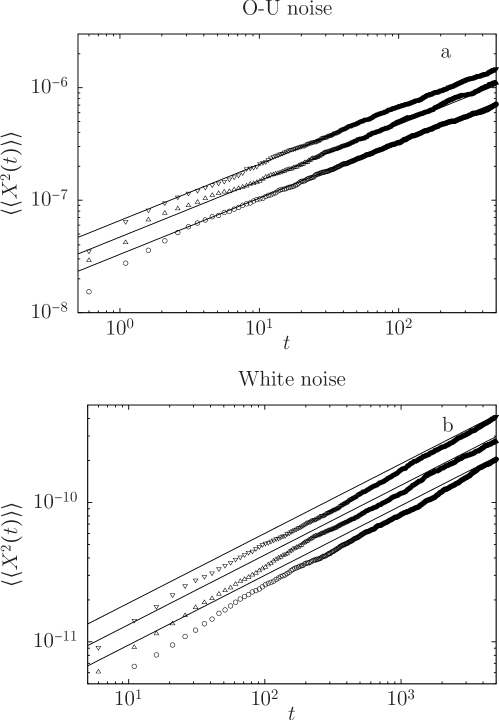
Figure 1: MSD for different cases where the coupling functions has been taken as in Eq. (11) with $\ell=5\times 10^{-4}$. Panel a) Gaussian Ornstein-Uhlembeck noise, i.e., exponential correlation function $\gamma(t)=\sigma^{2}e^{-t/\tau}/2\tau$ and intensity $D_{y}=\sigma^{2}/4\tau^{2}$. The symbols represent numerical simulations for different values of the noise intensity; circles: $D_{y}=1$, triangles: $D_{y}=0.25$, and inverted triangles: $D_{y}=1/16$. Panel b) Gaussian white noise with $D_{y}=1$ (circles), $D_{y}=0.5$ (triangles), and $D_{y}=1/4$ (inverted triangles). In both panels, $\beta_{x}=0.5$ and $D_{x}=1$. The straight solid lines correspond to the theoretical predictions given by Eq. (35)

Figure 1 confirms the result provided by Eq. (35), which implies that the MSD grows like $\sqrt{t}$ for long times for any Gaussian noise, regardless its correlation function. We have shown that subdiffusive transport with anomalous exponent 1/2 emerges under more general circumstances, namely if the motion in the $x$-direction, i.e., along the backbone, is driven by any white noise and the motion along the teeth is driven by any colored Gaussian noise with nonzero intensity.

V.2 Non-Gaussian White External Noise

We assume now that the particles move along the teeth driven by non-Gaussian noise, so-called Lévy noise. This noise in white in time, i.e., the autocorrelation function is $\left\langle\xi_{y}(t)\xi_{y}(t^{\prime})\right\rangle=\delta(t-t^{\prime})$. Then $\xi_{y}(t)$ is the time derivative of a generalized Wiener process $Y(t)$, i.e., $Y(t)=\int_{0}^{t}\xi_{y}(t^{\prime})dt^{\prime}$, see Eq.  (27). The random process $Y(t)$ has stationary independent increments on non-overlapping intervals Dubkov and Spagnolo (2005); Denisov et al. (2009). It belongs to the class of Lévy processes, and its PDF belongs to the class of infinitely divisible distributions. The characteristic functional of $Y(t)$ can be written in the form Dubkov and Spagnolo (2005)

$$\Phi(k,t)=\exp\left[t\int_{-\infty}^{\infty}dz\rho(z)\frac{e^{ikz}-1-ik\sin(z)}{z^{2}}\right].$$ (36)

Gaussian white noise corresponds to the kernel $\rho(z)=2\delta(z)$. Symmetric Lévy-stable noise with index $\theta$ corresponds to the power-law kernel $\rho(z)\sim\left\lvert z\right\rvert^{1-\theta}$ with $0<\theta<2$, which yields

$$\Phi(k,t)=\exp\left(-tD_{\theta}\left\lvert k\right\rvert^{\theta}\right),$$ (37)

where $D_{\theta}$ is a generalized diffusion coefficient. Substituting this expression for $\Phi(k,t)$ into Eq. (29) we obtain

$$\langle\langle X^{2}(t)\rangle\rangle\sim\begin{cases}\ln(t),&\theta=1,\\[4.30554pt] t^{1-1/\theta},&1<\theta\leq 2,\\[4.30554pt] O(1),&0<\theta<1,\end{cases}$$ (38)

as $t\to\infty$. If $\theta=2$, the characteristic functional (37) corresponds to the Gaussian one, and from (38) the MSD grows like $t^{1/2}$, as expected. For $1<\theta<2$, the MSD displays subdiffusive behavior, and the anomalous exponent decreases as $\theta$ decreases from 2 to 1. When it reaches the value $\theta=1$, Cauchy functional, the MSD grows ultraslowly. This behavior has been observed before Forte et al. (2013); Boyer and Solis-Salas (2014), but it appears here as a result of specific values of the characteristic parameters of the noise that drives the motion along the teeth. Finally, if $0<\theta<1$, the exponent is negative and the MSD approaches a constant value as time goes to infinity, i.e., stochastic localization or transport failure occurs.

Figure 2: MSD for three different values of the exponent $\theta$. Monte Carlo simulations correspond to $\theta=1$ (circles), $\theta=1.5$ (triangles), and $\theta=0.5$ (inverted triangles). Solid lines correspond to the theoretical predictions given by Eq. (38)

In Figure 2 we compare the analytical results provided by Eq. (38) with Monte Carlo simulations. Numerical and theoretical predictions show very good agreement for large $t$, where the results given by Eq. (38) hold.

V.3 Gaussian White Noise Along $n$-Dimensional Teeth

Finally we consider a ramified structure consisting of a unidimensional backbone intersected by $n$-dimensional secondary branches at the same point $(x=ia,y_{l}=0)$, where $l=1,...,n$. To deal with the stochastic dynamics, we consider Eq. (4a) together with the set of Langevin equations

$$\frac{dY_{l}}{dt}=\xi_{y_{l}}(t).$$ (39)

Proceeding similarly as for the case $l=1$ and taking into account $\langle\xi_{x}(t)\xi_{x}(t^{\prime})\rangle=2D_{x}\delta(t-t^{\prime})$, we find

$$\frac{dX^{2}}{dt}=2D_{x}\beta_{x}^{2}\prod_{l=1}^{n}[C_{l}(Y_{l})]^{2}.$$ (40)

Averaging over $Y_{1},\dotsc,Y_{n}$ yields

$$\frac{d}{dt}\left\langle\left\langle X^{2}(t)\right\rangle\right\rangle=2D_{x}\beta_{x}^{2}\prod_{l=1}^{n}\int_{-\infty}^{\infty}(C_{l}[y_{l}])^{2}P_{Y_{l}}(y_{l},t)dy_{l}.$$ (41)

We assume again that the dynamics of $X(t)$ and $Y_{l}(t)$ are coupled within a narrow strip of width $\ell$ around the backbone, i.e., the coupling function $C_{l}[y_{l}]$ has the form given by Eq. (11).

Integration of Eq. (41) yields, in the limit $\ell\rightarrow 0$,

$$\left\langle\left\langle X^{2}(t)\right\rangle\right\rangle=2D_{x}\beta_{x}^{2}\int_{0}^{t}\prod_{l=1}^{n}P_{Y_{l}}(0,t^{\prime})dt^{\prime}.$$ (42)

As in Eq. (28), $P_{Y_{l}}(k_{l},t)=\langle\exp[ik_{l}Y_{l}(t)]\rangle$. Integrating Eq. (39), we find the characteristic functional for each $\xi_{y_{l}}$,

$$\Phi(k_{l},t)=\left\langle\exp\left(ik_{l}\int_{0}^{t}\xi_{y_{l}}(t^{\prime})dt^{\prime}\right)\right\rangle,$$ (43)

and Eq. (29) now reads

$$\left\langle\left\langle X^{2}(t)\right\rangle\right\rangle=\frac{2D_{x}\beta_{x}^{2}}{(2\pi)^{n}}\int_{0}^{t}dt^{\prime}\prod_{l=1}^{n}\int_{-\infty}^{\infty}dk_{l}\Phi(k_{l},t^{\prime}).$$ (44)

We consider the case that the $\xi_{y_{l}}(t)$ are uncorrelated Gaussian white noises, i.e., $\langle\xi_{x_{m}}(t)\xi_{x_{l}}(t^{\prime})\rangle=2D_{y_{m}}\delta_{ml}\delta(t-t^{\prime})$, where $m,l=1,\dotsc,n$. Their characteristic functional is $\Phi(k_{l},t)=\exp(-tD_{y_{l}}k_{l}^{2})$. Substituting this result into Eq. (44), we find

$$\left\langle\left\langle X^{2}(t)\right\rangle\right\rangle\sim\begin{cases}t^{1/2},&n=1,\\[4.30554pt] \ln(t),&n=2,\\[4.30554pt] O(1),&n>2.\end{cases}$$ (45)

Note that the transport shows behavior similar to that of a comb with fractal teeth, see Sec. IV.3.

VI Secondary branches with finite length

If the range $\mathcal{D}$ of $Y(t)$ corresponds to a finite interval, it is convenient to work directly with Eq. (12), particularly if the dynamics on the secondary branches is described by a diffusion equation. As an example consider the case of normal diffusion described by the equation $\partial_{t}P_{Y}=D_{y}\partial_{yy}P_{Y}$ along one-dimensional branches in the $y$-direction of length $2L$ with reflecting boundary conditions, $(\partial_{y}P_{Y})_{y=\pm L}=0$, and initial condition $P_{Y}(y,0)=\delta(y)$. The solution $P_{Y}(y,t)$ is given by the Fourier series expansion

$$P_{Y}(y,t)=\frac{1}{2L}+\frac{1}{L}\sum_{n=1}^{\infty}\exp\left(-\frac{n^{2}\pi^{2}D_{y}}{L^{2}}t\right)\cos\left(\frac{n\pi y}{L}\right).$$ (46)

By inserting (46) into (12) we find after some algebra

$$\langle\langle X^{2}(t)\rangle\rangle=\frac{\beta_{x}^{2}D_{x}}{L}t+\frac{\beta_{x}^{2}D_{x}L}{3D_{y}}-\frac{2\beta_{x}^{2}D_{x}L}{\pi^{2}D_{y}}\sum_{n=1}^{\infty}n^{-2}\exp\left(-\frac{n^{2}\pi^{2}D_{y}}{L^{2}}t\right)$$ (47)

Consequently in the limit $t\to\infty$

$$\langle\langle X^{2}(t)\rangle\rangle\simeq\frac{\beta_{x}^{2}D_{x}}{L}t,$$ (48)

i.e., transport through the comb is normal diffusion as expected.

We compare this result with the case where the diffusion along the teeth is anomalous. The equation for subdiffusion along one-dimensional branches in the $y$-direction of length $2L$ is given by the fractional diffusion equation $\partial_{t}P_{Y}={}_{0}\mathcal{D}_{t}^{1-\alpha}K_{\alpha}\partial_{y}^{2}P_{Y},$ where ${}_{0}\mathcal{D}_{t}^{-\alpha}$ is the Riemann-Liouville fractional derivative with $0<\alpha<1$ Metzler and Klafter (2000) and $K_{\alpha}$ is a generalized diffusion coefficient. The solution $P_{Y}(y,t)$ is given by

$$P_{Y}(y,t)=\frac{1}{2L}+\frac{1}{L}\sum_{n=1}^{\infty}E_{\alpha}\left(-\frac{n^{2}\pi^{2}K_{\alpha}}{L^{2}}t^{\alpha}\right)\cos\left(\frac{n\pi y}{L}\right),$$ (49)

where $E_{\alpha}(z)$ is the Mittag-Leffler function. Using Eqs. (12) and (49), $E_{\alpha}(z)=E_{\alpha,1}(z)$, and the integration formula Podlubny (1999)

$$\int_{0}^{t}d\tau E_{\alpha,\beta}\left(\lambda\tau^{\alpha}\right)\tau^{\beta-1}=t^{\beta}E_{\alpha,\beta+1}\left(\lambda t^{\alpha}\right),$$ (50)

we obtain the MSD

$$\langle\langle X^{2}(t)\rangle\rangle=\frac{\beta_{x}^{2}D_{x}t}{L}+\frac{2\beta_{x}^{2}D_{x}t}{L}\sum_{n=1}^{\infty}E_{\alpha,2}\left(-\frac{n^{2}\pi^{2}K_{\alpha}t^{\alpha}}{L^{2}}\right),$$ (51)

where $E_{\alpha,\beta}(z)$ is the Generalized Mittag-Leffler function. The long-time behavior of the Mittag-Leffler function is given by Bateman (1953)

$$E_{\alpha,2}\left(-\frac{n^{2}\pi^{2}K_{\alpha}t^{\alpha}}{L^{2}}\right)\sim\frac{L^{2}}{\Gamma(2-\alpha)n^{2}\pi^{2}K_{\alpha}t^{\alpha}},$$ (52)

and the MSD reads

$$\langle\langle X^{2}(t)\rangle\rangle=\frac{\beta_{x}^{2}D_{x}}{L}t+\frac{\beta_{x}^{2}D_{x}L}{3\Gamma(2-\alpha)K_{\alpha}}t^{1-\alpha},$$ (53)

where we have used $\sum_{n=1}^{\infty}1/n^{2}=\pi^{2}/6$. It is clear that for $t\rightarrow\infty$ the first term of the right hand side of (53) is dominant and the MSD displays normal diffusive behavior.

Having studied the effect of subdiffusion in finite-length teeth, we now consider the case where particles perform superdiffusive motion in the teeth. The equation for $P_{Y}(y,t)$ is given by $\partial_{t}P_{Y}=D_{\mu}\partial_{y}^{\mu}P_{Y}$ with $1<\mu<2$ and with the same boundary and initial conditions as in the previous cases. Superdiffusion is described by the fractional derivative $\partial_{y}^{\mu}$, which corresponds to a heavy-tailed jump length PDF, and $D_{\mu}$ is a generalized transport coefficient. The eigenvalue problem $\partial_{y}^{\mu}\psi_{n}(y)=e_{n}\psi_{n}(y)$ has been considered in Iomin (2015). The Lévy operator in a box of size $2L$ reads

$$\partial_{y}^{\mu}f(y)=\int_{-L}^{L}\left[\frac{1}{2\pi}\int_{-\infty}^{\infty}(-\lvert k\rvert^{\mu})e^{-ik(y-y^{\prime})}dk\right]f(y^{\prime})dy^{\prime}.$$ (54)

As it follows from Iomin (2015), the eigenfunctions are $\psi_{n}(y)=\cos(n\pi y/L)$, where $n=0,1,2,\dotsc$, with corresponding eigenvalues $e_{n}=-(\pi n/L)^{\mu}$. The PDF in the teeth reads now

$$P_{Y}(y,t)=\frac{1}{2L}+\frac{1}{L}\sum_{n=1}^{\infty}\exp\left(-\frac{n^{\mu}\pi^{\mu}D_{\mu}}{L^{\mu}}t\right)\cos\left(\frac{n\pi y}{L}\right).$$ (55)

Following the same steps to obtain (48) from (46) we find here the asymptotic result

$$\langle\langle X^{2}(t)\rangle\rangle=\frac{\beta_{x}^{2}D_{x}}{L}t\quad\text{as}\quad t\to\infty.$$ (56)

We have shown that the transport along the backbone is diffusive for finite length teeth, if the transport regime of the particles in the teeth is normal diffusion, subdiffusion, and superdiffusion.

The robustness of the diffusive behavior of the MSD along the backbone can be understood as follows. If the random motion of the particles along the finite teeth with reflecting boundary conditions is homogeneous and unbiased, then $P_{Y}(y,t)\to 1/(2L)$ as $t\to\infty$. The function system

$$\frac{1}{\sqrt{2L}},\,\frac{1}{\sqrt{L}}\cos\left(\frac{n\pi y}{L}\right),\quad n=1,2,\dotsc,$$ (57)

is a complete orthonormal system on $[-L,L]$. Consequently, the PDF of the particle motion along the teeth, with initial condition $P_{Y}(y,0)=\delta(y)$, can be written as

$$P_{Y}(y,t)=\frac{1}{2L}+\frac{1}{L}\sum_{n=1}^{\infty}T_{n}(t)\cos\left(\frac{n\pi y}{L}\right),$$ (58)

with $T_{n}(0)=1$ and $T_{n}(t)\to 0$ as $t\to\infty$. If $T(t)\equiv\sum_{n=1}^{\infty}T_{n}(t)$ is well-defined, i.e., the series converges, for $t$ sufficiently large and if there exists a constant $C$ with $0\leq C<\infty$, such that $(1/t)\int_{0}^{t}dt^{\prime}T(t^{\prime})\to C$ as $t\to\infty$, then the MSD displays again normal diffusive behavior. These conditions are satisfied for the three cases analyzed above. In other words, if the teeth are finite , then the reflecting boundary conditions will give rise to a uniform distribution along the teeth for all types of transport. That is, the nature of the transport, anomalous or not, plays no role. This is due to a balance reached between particles within the teeth and those in the backbone. Although subdiffusive transport in the teeth makes that mean residence times within the teeth can diverge, this is balanced by the fact that typical times of departure from the backbone also diverge asymptotically with the same anomalous exponent. So, both effects compensate to keep $P_{Y}(y=0,t)$ constant asymptotically for large times, so the MSD will grow linearly in time according to Eq. (12). In the Appendix we provide a more formal justification of this idea by studying the asymptotic behavior of $P_{Y}(y=0,t)$ as a function of the backbone-teeth time dynamics. Therefore, since the transport along the backbone itself is diffusive, being driven by white noise, we expect to obtain a diffusive scaling for the MSD.

VII Conclusions

We have adopted a general Langevin formalism to explore transport through ramified comb-like structures. The transport through the structure is characterized by the behavior of the MSD along the backbone. We have derived an exact analytical expression, given in Eqs. (12) – (14), that allows us to determine the MSD explicitly from the PDF of the motion along the secondary branches, $P_{Y}(y,t)$, i.e., the probability of a particle to be at point $y$ of a secondary branch at time $t$.

If the secondary branches have finite length and reflecting boundary conditions, then under some mild conditions the transport regime along the teeth does not matter and the MSD is proportional to $t$, indicating standard diffusion. We have shown this explicitly for diffusive, subdiffusive, and superdiffusive motion along the secondary branches. If the secondary branches have infinite length, then both subdiffusion and superdiffusion along the teeth generate a subdiffusive MSD along the backbone. Therefore, the finite or infinite length of the secondary branches plays a crucial role for the transport along the overall structure.

Another interesting situation arises if the dynamics of the particles along the secondary branches are described directly by a Langevin equation. For this case we have obtained an exact analytical formula, see Eq. (29), that relates the MSD along the backbone to the characteristic functional of the noise $\xi_{y}(t)$ driving the motion along the secondary branches. This expression is completely general and holds for any noise $\xi_{y}(t)$. We have considered several different situations. For Gaussian colored noise $\xi_{y}(t)$, we have shown that if the noise intensity is finite and nonzero, then the MSD grows like $t^{1/2}$ along the backbone. We have checked this result with Monte Carlo simulations, performed for the case of Gaussian white noise and exponentially correlated Gaussian noise, i.e., Ornstein-Uhlenbeck noise. In addition, we have also considered that $\xi_{y}(t)$ is white but non-Gaussian noise. In this case our interest has been focused on symmetric Lévy-stable noise with exponent $\theta$. We have found that the MSD along the backbone grows ultraslowly like $\ln(t)$, if the PDF of the white noise $\xi_{y}(t)$ is a Cauchy distribution, $\theta=1$. For $0<\theta<1$, the MSD exhibits stochastic localization, i.e., it approaches asymptotically a constant value, while for $1<\theta<2$ the MSD exhibits subdiffusion. Excellent agreement is found with Monte Carlo simulations. We have also considered multidimensional and fractal secondary branches. We have obtained different behaviors like ultraslow motion, subdiffusion, and stochastic localization in terms of the dimension of the secondary branches.

In summary, we have shown in this work how particles moving through a simple regular structure, namely a comb, are able to display a variety of macroscopic transport regimes, namely transport failure (stochastic localization), subdiffusion, or ultraslow diffusion, depending on whether the secondary branches have finite or infinite length but also on the statistical properties of the noise that drives the motion along them. We expect our results to find applications to the description of the movement of organisms and animals through ramified structures like river networks, ecological corridors, etc.

Appendix

In Section VI we have seen that diffusive properties in the backbone do not change qualitatively by introducing different modes of transport (superdiffusive, subdiffusive) within the teeth. Intuitively, one expects that the transport properties in the backbone are mainly determined by the dynamics of entrance within the teeth and return from it (since only particles at $y=0$ contribute to the transport in the backbone).

To clarify this connection, we here derive the dependence of $P_{Y}(y=0,t)$ (which determines the mean square displacement through Eq. (12)) with the typical times the particle stays in the teeth. We introduce $\psi_{1}(t)$ as the probability distribution of times a particle stays in the backbone before entering into the teeth, and $\psi_{2}(t)$ as the corresponding distribution of times the particle spends within the teeth before returning to the backbone. So, the mean value of $\psi_{2}(t)$ determines the mean residence time within the teeth. The probability that a particle is at $y=0$ at an arbitrary time $t$ will be then given by

$$P_{Y}(y=0,t)=\Psi_{1}(t)+\psi_{1}(t)*\psi_{2}(t)*\Psi_{1}(t)+\psi_{1}(t)*\psi_{2}(t)*\psi_{1}(t)*\psi_{2}(t)*\Psi_{1}(t)+\ldots$$ (59)

where $\Psi_{1}(t)$ is the survival probability of $\psi_{1}(t)$, i.e. $\Psi_{1}(t)=\int_{t}^{\infty}\psi_{1}(t^{\prime})dt^{\prime}$, and the asterisk denotes time convolution; also, we have here implicitly assumed that at $t=0$ all the particles are located in the backbone, $P_{Y}(y=0,0)=1$. In the previous expression, the first term on the rhs represents those particles which have not left yet the backbone at time $t$, the second term corresponds to those that are currently at the backbone after a previous excursion within the teeth, the third term represents those particles that have performed two previous excursions within the teeth, and so on.

Using Laplace transform to deal easily with the time convolution operators, we find

$$\hat{P_{Y}}(y=0,s)=\frac{\hat{\Psi_{1}}(s)}{1-\hat{\psi_{1}}(s)\hat{\psi_{2}}(s)}$$ (60)

where the hat denotes the Laplace transform, and $s$ is the Laplace argument.

Now that we have reached a generic expression connecting the backbone-teeth time dynamics to $\hat{P}_{Y}(y=0,s)$, we can study how this expression behaves in the long-time (or equivalently, small $s$) regime. For this, we assume that the distributions of times within the backbone and within the teeth follow generic anomalous scaling in the asymptotic regime through $\psi_{1}(t)\sim t^{-1-\alpha_{1}}$ and $\psi_{2}(t)\sim t^{-1-\alpha_{2}}$, for $t\rightarrow\infty$. With the help of Tauberian theorems we can translate this to Laplace space and obtain finally from (60)

$$\lim_{s\rightarrow 0}\hat{P_{Y}}(y=0,s)\sim s^{\alpha_{1}-1-\min(\alpha_{1},\alpha_{2})}$$ (61)

This expression confirms our results above in Section VI. If the anomalous exponent determining the entrance within the teeth and the return from it satisfies $\alpha_{1}\leq\alpha_{2}$ then we get $\lim_{s\rightarrow 0}\hat{P}_{Y}(y=0,s)\sim s^{-1}$, or equivalently $\lim_{t\rightarrow\infty}P_{Y}(y=0,t)\sim\mathrm{const}$, and then the transport in the backbone is always diffusive independent of $\alpha_{i}$ with $i=1,2$. This will be the case for normal diffusion within the teeth, and also for anomalous transport within the teeth determined by power-law asymptotic decay of waiting times (see, e.g. Metzler and Klafter (2004), for details and a deeper discussion on this point). Additionally, we observe from (61) that only in the case of an imbalance in the backbone-teeth dynamics (so $\alpha_{1}>\alpha_{2}$) we could obtain a different (non-diffusive) result.

References

- Rodríguez-Iturbe and Rinaldo (1997) I. Rodríguez-Iturbe and A. Rinaldo, Fractal River Basins: Chance and Self-Organization (Cambridge University Press, Cambridge, 1997).
- Bertuzzo et al. (2010) E. Bertuzzo, R. Casagrandi, M. Gatto, I. Rodriguez-Iturbe, and A. Rinaldo, J. R. Soc. Interface 7, 321 (2010).
- Muneepeerakul et al. (2008) R. Muneepeerakul, E. Bertuzzo, H. J. Lynch, W. F. Fagan, A. Rinaldo, and I. Rodriguez-Iturbe, Nature 453, 220 (2008).
- Forte et al. (2013) G. Forte, R. Burioni, F. Cecconi, and A. Vulpiani, J. Phys.: Condens. Matter 25, 465106 (2013).
- Méndez et al. (2010) V. Méndez, S. Fedotov, and W. Horsthemke, Reaction-Transport Systems: Mesoscopic Foundations, Fronts and Spatial Instabilities (Springer, Heidelberg, 2010).
- Weiss and Havlin (1986) G. H. Weiss and S. Havlin, Physica A 134, 474 (1986).
- White and Barma (1984) S. R. White and M. Barma, J. Phys. A: Math. Gen. 17, 2995 (1984).
- Arkhincheev and Baskin (1991) V. E. Arkhincheev and E. M. Baskin, Sov. Phys. JETP 73, 161 (1991).
- Méndez and Iomin (2013) V. Méndez and A. Iomin, Chaos, Solitons & Fractals 53, 46 (2013).
- Iomin and Méndez (2013) A. Iomin and V. Méndez, Phys. Rev. E 88, 012706 (2013).
- Fedotov and Méndez (2008) S. Fedotov and V. Méndez, Phys. Rev. Lett. 101, 218102 (2008).
- Frauenrath (2005) H. Frauenrath, Prog. Polymer Sci. 30, 325 (2005).
- Arkhincheev (1999) V. E. Arkhincheev, J. Exp. Theor. Phys. 88, 710 (1999).
- Baskin and Iomin (2004) E. Baskin and A. Iomin, Phys. Rev. Lett. 93, 120603 (2004).
- Bel and Nemenman (2009) G. Bel and I. Nemenman, New J. Phys. 11, 083009 (2009).
- Ribeiro et al. (2014) H. V. Ribeiro, A. A. Tateishi, L. G. A. Alves, R. S. Zola, and E. K. Lenzi, New J. Phys. 16, 093050 (2014).
- Montroll and Weiss (1965) E. W. Montroll and G. H. Weiss, J. Math. Phys. 6, 167 (1965).
- Havlin and ben Avraham (1987) S. Havlin and D. ben Avraham, Adv. Phys. 36, 695 (1987).
- Bertacchi (2006) D. Bertacchi, Electron. J. Probab. 11, 1184 (2006).
- Méndez et al. (2015) V. Méndez, A. Iomin, D. Campos, and W. Horsthemke, Phys. Rev. E 92 (2015), 10.1103/PhysRevE.92.062112.
- Lutz (2001) E. Lutz, Phys. Rev. E 64, 051106 (2001).
- Mosco (1997) U. Mosco, Phys. Rev. Lett. 79, 4067 (1997).
- Denisov and Horsthemke (2000) S. I. Denisov and W. Horsthemke, Phys. Rev. E 62, 7729 (2000).
- Klyatskin (2005) V. I. Klyatskin, Stochastic equations through the eye of the physicist: Basic concepts, exact results and asymptotic approximations (Elsevier, 2005).
- Hänggi and Jung (1995) P. Hänggi and P. Jung, Advances in chemical physics 89, 239 (1995).
- Dubkov and Spagnolo (2005) A. Dubkov and B. Spagnolo, Fluct. Noise Lett. 5, L267 (2005).
- Denisov et al. (2009) S. I. Denisov, W. Horsthemke, and P. Hänggi, Eur. Phys. J. B 68, 567 (2009).
- Boyer and Solis-Salas (2014) D. Boyer and C. Solis-Salas, Phys. Rev. Lett. 112, 240601 (2014).
- Metzler and Klafter (2000) R. Metzler and J. Klafter, Phys. Rep. 339, 1 (2000).
- Podlubny (1999) I. Podlubny, Fractional Differential Equations (Academic Press, San Diego, 1999).
- Bateman (1953) H. Bateman, Higher Transcendental Functions, Vol. III (McGraw-Hill, New York, 1953).
- Iomin (2015) A. Iomin, Chaos, Solitons & Fractals 71, 73 (2015).
- Metzler and Klafter (2004) R. Metzler and J. Klafter, Journal of Physics A: Mathematical and General 37, R161 (2004).