Density inhomogeneities and Rashba spin-orbit coupling interplay in oxide interfaces

Abstract

There is steadily increasing evidence that the two-dimensional electron gas (2DEG) formed at the interface of some insulating oxides like LaAlO₃/SrTiO₃ and LaTiO₃/SrTiO₃ is strongly inhomogeneous. The inhomogeneous distribution of electron density is accompanied by an inhomogeneous distribution of the (self-consistent) electric field confining the electrons at the interface. In turn this inhomogeneous transverse electric field induces an inhomogeneous Rashba spin-orbit coupling (RSOC). After an introductory summary on two mechanisms possibly giving rise to an electronic phase separation accounting for the above inhomogeneity, we introduce a phenomenological model to describe the density-dependent RSOC and its consequences. Besides being itself a possible source of inhomogeneity or charge-density waves, the density-dependent RSOC gives rise to interesting physical effects like the occurrence of inhomogeneous spin-current distributions and inhomogeneous quantum-Hall states with chiral “edge” states taking place in the bulk of the 2DEG. The inhomogeneous RSOC can also be exploited for spintronic devices since it can be used to produce a disorder-robust spin Hall effect.

I Introduction

After a two-dimensional electron gas (2DEG) was detected at the interface between two insulating oxides ohtomo-2004 , an increasingly intense theoretical and experimental investigation has been devoted to these systems. The properties of this 2DEG are intriguing for several reasons. The 2DEG can be made superconducting when its carrier density is tuned by means of gate voltage, both in LaAlO₃/SrTiO₃ (henceforth, LAO/STO) reyren-2007 ; caviglia-2008 and LaTiO₃/SrTiO₃ (henceforth, LTO/STO) biscaras-2010 ; biscaras-2012 interfaces, thus opening the way to voltage-driven superconducting devices. Also, it exhibits magnetic propertiesariando-2010 ; lilu-2011 ; bert-2011 ; dikin-2011 ; metha-2012 ; bert-2012 , displays a strong and tunablecaviglia-2012 ; ben-shalom-2010 ; caprara-2012 ; hurand-2015 Rashba spin-orbit couplingrashba-1984 , and it is extremely two-dimensional, having a lateral extension $\sim 5$ nm. Magnetotransport experiments reveal the presence of high- and low-mobility carriers in LTO/STO, and superconductivity seems to develop as soon as high-mobility carriers appearbiscaras-2012 ; bell-2009 , when the carrier density is tuned above a threshold value by means of gate voltage, $V_{g}$. When the temperature $T$ is lowered, the electrical resistance is reduced, and signatures of a superconducting fraction are seen well above the temperature at which the global zero resistance state is reached (if ever). The superconducting fraction decreases with decreasing $V_{g}$, although a superconducting fraction survives at values of $V_{g}$ such that the resistance stays finite down to the lowest measured temperatures. When $V_{g}$ is further reduced, the superconducting fraction eventually disappears, and the 2DEG stays metallic at all temperatures and seems to undergo weak localization at low $T$. At yet smaller carrier densities, the system behaves as an insulator. The width of the superconducting transition is anomalously large and it cannot be accounted for by reasonable superconducting fluctuationscaprara-2011 . This phenomenology suggests instead that an inhomogeneous 2DEG is formed at these oxide interfaces, consisting of superconducting “puddles” embedded in a weakly localizing metallic background, opening the way to a percolative superconducting transitionbucheli-2013 . Inhomogeneities are revealed in various magnetic experimentsariando-2010 ; lilu-2011 ; bert-2011 ; dikin-2011 ; metha-2012 ; bert-2012 ; Prawiroatmodjo-2016 , in tunneling spectraristic-2011 , and in piezoforce microscopy measurementsfeng-bi-2013 . Specific informations on the doping and temperature dependence of the inhomogeneity in these systems have been recently extracted from a theoretical analysisbucheli-2015 of tunnelling experimentsrichter-2013 . The inhomogeneous structure of these systems is rather complex. On the one hand, large micrometric-scale inhomogeneities have been revealed by the occurrence of striped textures in the current distributionkalisky-2013 and in the surface potentialhonig-2013 . On the other hand, experiments investigating the quantum critical behavior of the superconductor-(weakly localized) metal transitionbiscaras-2013 , transport experiments in nanobridgesnanobridges , and piezo-force experimentsfeng-bi-2013 indicate that inhomogeneities have a finer structure extending down to nanometric scales. The inhomogeneous character of these oxide interfaces (henceforth referred to as LXO/STO interfaces, when referring to both LAO/STO and LTO/STO) has been extensively discussed in phenomenological analyses of transport experimentscaprara-2013 ; caprara-2015 . The very inhomogeneous character (especially at small scales) also calls for some intrinsic mechanisms promoting the inhomogeneous distribution of electron density. The possibility of an electronic phase separation (EPS) in these materials has indeed been considered and two, possibly cooperative, mechanisms have been identified. In Sect. II, after a short presentation of the electronic structure of LXO/STO interfaces, we will briefly reconsider these mechanisms for EPS both for the sake of completeness and to introduce the model that will be the main focus of this paper: the density-dependent Rashba spin-orbit coupling (RSOC). In this model the RSOC is assumed to depend on the local electric field, which in turn is a monotonically increasing function of the local electron density. Therefore, where the electron density is larger, also the local confining electric field perpendicular to the interface is larger, thereby inducing a stronger RSOC. The subsequent sections will instead be devoted to the analysis of the remarkable consequences of this inhomogeneous distribution of electron density and RSOC.

II Two mechanisms for electronic instabilities in LXO/STO

Photoemission spectroscopy clearly indicates that the valence band of STO and of the LXO overlayer align themselves and the excess electrons at the interface are accommodated in the potential well formed by the STO conduction band bending, while the conduction band of the overlayer is well abovetreske-2015 . This well, which is some tens of eV deep ($>0.4$ eV), gives rise to a quantum confinement of the electrons in the $z$ direction perpendicular to the LXO/STO interface and the interfacial electron gas acquires a strong two-dimensional character. Thus the 2DEG resides on the STO side and it occupies the $t_{2g}$ orbitals ($d_{xy},d_{xz},d_{yz}$) of the STO conduction band. The different orientation and overlap of the orbitals in the ($xy$) and $z$ directions has important consequences in the electronic structure of the quantized sub-bands. The $d_{xy}$ orbitals have small overlap along $z$ and give rise to a band with small dispersion (heavy mass $m_{H}\sim 20m_{0}$, where $m_{0}$ is the free electron mass) along this direction. Therefore, when quantum confinement is enforced, the sub-band levels are relatively closely spaced. On the other hand, the $d_{xz,yz}$ orbitals have a substantial overlap in the $z$ direction and would give rise to dispersed bands (and light masses, $m_{L}\sim 0.7m_{0}$), were it not for the confinement. Then the quantized sub-bands are much more widely spaced and the first occupied level is $50-100$ meV above the lowest sub-bands of $d_{xy}$ origin. Both XAS experimentssalluzzo-2009 and first-principle calculations popovic-2008 ; delugas-2011 ; zhong-2013 agree on this electronic scheme.

II.1 Phase separation instability in confined electrons at LXO/STO interfaces

The thermodynamic stability of the LXO/STO systems was recently investigatedscopigno-2016 in order to identify a possible mechanism for EPS. In particular the system was schematized as in Fig. 1, where the thin LXO overlayer is positively charged because of the countercharges (due to the polarity-catastrophe mechanismnakagawa-2006 ; liping-yu-2014 and/or to oxygen vacancies) left by the electrons transferred to the STO interface region. These transferred electrons either occupy discrete levels in the potential well, which form mobile 2D bands along the $x,y$ directions or are trapped in more deeply localized states inside the STO layer.

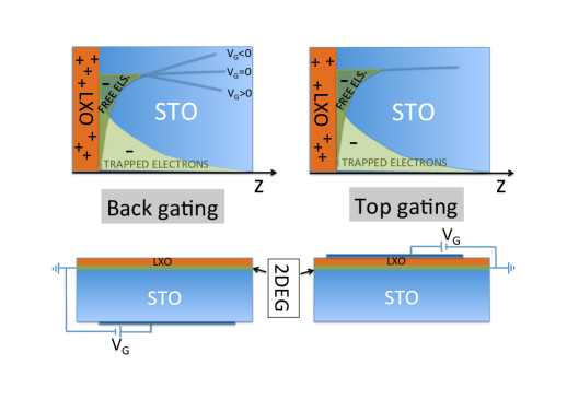
Figure 1: Sketch of the interface for back (a) and top (b) gating. The upper part sketches the confining potentials, while the bottom part reports the structure of samples and electrodes. The confining potential depends on both mobile (dark green shade) and trapped (light green shade) charges, which together compensate the positive counter-charges $n$ in the LXO side. Applying a positive (negative) voltage electrons are added to (subtracted from) the interface and the potential changes accordingly.

The electrostatic configuration of the system is also determined by the metallic gates that are under the STO substrate (back gating) and/or above the LXO overlayer (top gating), tuning the electron density. The stability of the electronic state was investigated by varying the density of the interfacial gas while keeping the overall neutrality. Therefore, a corresponding amount of positive countercharges has to be varied (see Fig. 1). Because of this tight connection between positive and negative charges the (in)stability will be determined by calculating the chemical potential of the whole system (i.e., of both the mobile electrons and of the other charges). While we will solve the quantum problem of the mobile electrons in the self-consistent confining well, the countercharges, the fraction of electrons trapped in impurity states of the bulk (see below), and the boundary conditions fixing the gating potential will determine the classical electrostatic energy of the system. All these contributions (see Ref. scopigno-2016, ) yield the total energy $E$ and, in turn, the chemical potential $\mu=E(N+1)-E(N)\approx\partial_{N}E$ (here $N$ represents the number of electrons, which is always kept equal to the number of countercharges). The mobile electron density along $z$ and the spectrum of the discrete levels was determined by solving the Schrödinger equation along the $z$ direction, while the corresponding electrostatic potential was found by solving the Poisson equation. By iteratively solving these two equations the self-consistent potential well and the electronic states were determined, providing the total energy of the system (also including all electrostatic contributions arising from positive countercharges, gate electric fields, trapped localized electrons). From this the chemical potential evolution with the electron density $n$ was found, as reported in Fig. 2.

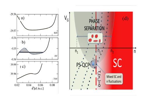
Figure 2: (a-c) Chemical potential as a function of the mobile electron density at fixed values of the back-gating potential $V_{g}$ (the electrons due to gating are thus also fixed) in the presence of a short-range background contribution to the chemical potential accounting for the short-range rigidity of the countercharges (see Ref.scopigno-2016, ) In (b) an example of Maxwell construction is given, with the gray shaded areas being equal. (d) Sketch of the phase diagram with the phase separation region (gray) mixing the superconducting (red) and normal metallic (light green) phases. The thick red dashed line marks the critical filling at which SC sets in, while the dotted lines show how the total density varies in a back-gating configuration. The darker shaded area marks the The densities $n_{1}$ and $n_{2}$ delimit the miscibility gap.

It is clear that at some densities the chemical potential decreases upon increasing $n$, thereby signaling a negative compressibility that marks the EPS. The boundaries of the coexistence region are then determined by a standard Maxwell construction in full analogy with the liquid-gas transition. As a consequence, a density-vs-gate potential region is determined, where regions at different electron density coexist. Of course, the above treatment says nothing about the size of the minority droplets embedded in the majority phase: this is determined by specific, model-dependent ingredients like the interface energy of the droplets, the mobility of the countercharges that are needed to keep charge neutrality, and so on. Simple estimates show that the very large value of the dielectric constant of STO weakens the Coulomb repulsion and allows this frustrated EPS mechanism to produce rather large ($\sim 50$ nm) inhomogeneities. On the other hand, it is also possible that the positive countercharges (like the oxygen vacancies) diffuse and follow the segregating electrons keeping charge neutrality. Of course, also in this case, EPS stops when the segregating electrons become too dense for the countercharges to follow, but finite inhomogeneities of substantial size can still be formed. It is important to notice that the calculations find perfectly realistic density ranges in which the EPS occurs, with the high-density phases always reaching local electron densities sufficient to fill the higher orbitals $d_{xz,yz}$. Since these are associated to the high-mobility carriers responsible for superconductivity, it is quite natural to assume that the EPS creates puddles at higher-density where superconductivity takes place at low-enough temperature. These puddles are then the basic “bricks” giving rise to the inhomogeneous superconducting state discussed in Sect. I.

II.2 Phase separation instability in confined electrons with Rashba spin-orbit coupling

Before the quite effective mechanism for EPS presented in the previous subsection was identified, another mechanism was found and discussed based on the dependence of the RSOC self-consistent local electric field and, consequently, on the local density. Simple inspection of the electrostatic potential well confining the electrons (as obtained from the self-consistent Schrödinger-Poisson approach) shows that where the electron density is higher, the confining electric field is correspondingly higher (on the average in the well). Therefore the RSOC is also larger. Since RSOC brings along a lowering of the planar electronic spectrum (for free electrons, if the minimum of the parabolic dispersion is set to zero for $\alpha=0$, it becomes $-\varepsilon_{0}=-\alpha^{2}m/2$ for finite RSOC), the electron energy tends to be lower in the high-density regions. (see Fig. 3).

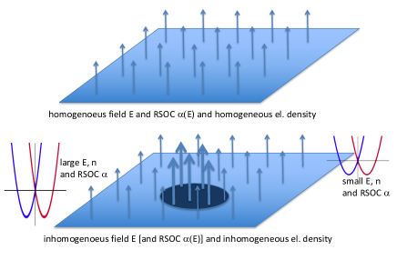
Figure 3: Schematic view of the 2DEG in the homogeneous case (above) where both electron density and transverse electric field (the arrows) are uniformly distributed. (Bottom) Inhomogeneous case where the electric field is larger where the electron density is higher (darker region). The schematic view of the electron spectrum is reported showing that the bottom of the band is lower when the RSOC is larger.

Of course, whether or not this is enough to induce an electronic instability, is a matter of numbers and the detailed analysis of this mechanismcaprara-2012 ; bucheli-2014 established that the DOS of electrons in the dispersive $d_{xy}$ bands is not large enough to cause an EPS, while the substantially larger DOS of the higher $d_{xz,yz}$ sub-bands might indeed induce this instability for values of the order (or just $30-40$ % larger) of those experimentally found in LXO/STO interfacescaviglia-2012 ; ben-shalom-2010 ; hurand-2015 . After the discovery of the more effective mechanism based on the electrostatic confinement (see the previous subsection), the safer attitude is perhaps to consider this mechanism as cooperative to strengthen the instability tendency in the 2DEG at the LXO/STO interfaces. Most interestingly, however, is that any inhomogeneous distribution of electron density (whatever the formation mechanisms might be) entails an inhomogeneous distribution of RSOC, with important consequences both from the fundamental and applicative points of view. The focus of this paper is precisely to present some of these important physical and applicative consequences of a density-related inhomogeneous RSOC.

III Rashba model with density dependent coupling

The basic features resulting from a density dependent RSOC can be elucidated from a single-band Rashba model on a lattice described by the hamiltonian

$$H = \sum_{ij\sigma}t_{ij}c^{\dagger}_{i\sigma}c_{j\sigma}+\sum_{ij\sigma\sigma^{\prime}}\left[g^{x}_{ij}\tau^{x}_{\sigma\sigma^{\prime}}+g^{y}_{ij}\tau^{y}_{\sigma\sigma^{\prime}}\right]c^{\dagger}_{i\sigma}c_{j\sigma^{\prime}}$$ (1)

$$+ \sum_{i,\sigma}\lambda_{i}\left[c^{\dagger}_{i\sigma}c_{i\sigma}-n_{i}\right]+\sum_{i\sigma}V_{i}c^{\dagger}_{i\sigma}c_{i\sigma}.$$

Here, the first term describes the kinetic energy of electrons on a square lattice (with lattice constant $a$) where we only take hopping between nearest-neighbors into account ($t_{ij}\equiv-t$ for $|R_{i}-R_{j}|=a$). The second term is the RSOC with $g_{ij}^{\alpha}=-g_{ji}^{\alpha}=-(g_{ij}^{\alpha})^{*}$. Since the coupling constants will be defined as density dependent, this results in a local coupling to charge density fluctuations with $n_{i}=\sum_{\sigma}\langle c^{\dagger}_{i\sigma}c_{i\sigma}\rangle$ and the $\lambda_{i}$ are determined self-consistently. The last term describes an external (impurity) potential with local energies $V_{i}$ which are drawn from a flat distribution with $-V_{0}\leq V_{i}\leq V_{0}$.

In our investigations the RSOC is also restricted to nearest-neighbor processes. We write the couplings as

$$g^{x}_{ij} = -\mathrm{i}\gamma_{ij}\left[\delta_{R_{j},R_{i+y}}-\delta_{R_{j},R_{i-y}}\right]$$

$$g^{y}_{ij} = -\mathrm{i}\gamma_{ij}\left[\delta_{R_{j},R_{i+x}}-\delta_{R_{j},R_{i-x}}\right]$$

so that the property $g_{ij}^{\alpha}=-g_{ji}^{\alpha}$ requires

$$\gamma_{ij}=\gamma_{ji}.$$ (2)

The coupling can be also written in the form

$$H^{RSO}=\sum_{i}\left[\gamma_{i,i+y}j_{i,i+y}^{x}-\gamma_{i,i+x}j_{i,i+x}^{y}\right]$$

where

$$j_{i,i+\eta}^{\alpha}=-\mathrm{i}\sum_{\sigma\sigma^{\prime}}\left[c^{\dagger}_{i\sigma}\tau^{\alpha}_{\sigma\sigma^{\prime}}c_{i+\eta,\sigma^{\prime}}-c^{\dagger}_{i+\eta,\sigma}\tau^{\alpha}_{\sigma^{\prime}\sigma}c_{i,\sigma}\right]$$

denotes the $\alpha$-component of the spin-current flowing on the bond between $R_{i}$ and $R_{i+\eta}$. Following Ref. caprara-2012, , we assume that the coupling constants depend on a perpendicular electric field $E{\bf e}_{z}$ which is proportional to the local charge density. Since in real space the coupling constants $g_{i,i+\eta}$ are defined on the bonds, we discretize the electric field at the midpoints of the bonds and define the dependence on the charge as

$$E_{i+\eta/2}=e_{0}+e_{1}(n_{i}+n_{i+\eta})\,.$$

For the dependence of the RSOC on the electric field we adopt the form given in Ref. caprara-2012, , so that altogether the following coupling is considered

$$\gamma_{i,i+\eta}=\frac{a_{0}+a_{1}(n_{i}+n_{i+\eta})}{[1+b_{0}+b_{1}(n_{i}+n_{i+\eta})]^{3}}\,,$$ (3)

which fulfills the property Eq. (2).

We show below that for strong RSOC this coupling will induce the formation of electronic inhomogeneities and thus concomitant variations in the local chemical potential $\lambda_{i}$. The latter can be obtained self-consistently by minimizing the energy which yields

$$\lambda_{i}=\frac{\partial g_{i,i+y}}{\partial n_{i}}\langle j_{i,i+y}^{x}\rangle-\frac{\partial g_{i,i+x}}{\partial n_{i}}\langle j_{i,i+x}^{y}\rangle\,.$$ (4)

III.1 Stability analysis

If we insert the Lagrange parameter in the hamiltonian Eq. (1) the energy functional reads as

$$E = E_{0}+\sum_{i\sigma}\left(\frac{\partial\gamma_{i,i+y}}{\partial n_{i}}\langle c^{\dagger}_{i\sigma}c_{i\sigma}\rangle+\frac{\partial\gamma_{i,i+y}}{\partial n_{i+y}}\langle c^{\dagger}_{i+y,\sigma}c_{i+y,\sigma}\rangle\right)\langle j_{i,i+y}^{x}\rangle$$ (5)

$$- \sum_{i\sigma}\left(\frac{\partial\gamma_{i,i+x}}{\partial n_{i}}\langle c^{\dagger}_{i\sigma}c_{i\sigma}\rangle+\frac{\partial\gamma_{i,i+x}}{\partial n_{i+x}}\langle c^{\dagger}_{i+x,\sigma}c_{i+x,\sigma}\rangle\right)\langle j_{i,i+x}^{y}\rangle$$

with

$$E_{0} = \sum_{ij\sigma}t_{ij}\langle c^{\dagger}_{i\sigma}c_{j\sigma}\rangle$$

$$+ \sum_{i}\left[\gamma^{0}_{i,i+y}\langle j_{i,i+y}^{x}\rangle-\gamma^{0}_{i,i+x}\langle j_{i,i+x}^{y}\rangle\right]$$

and the notation $\gamma^{0}=\gamma(n_{0})$ refers to the coupling at a given density $n_{0}$.

From Eq. (5) it becomes apparent that the density dependent coupling induces an effective density-current interaction. Assume that the problem has been solved for a given homogeneous density $n_{0}$ (in the following we take densities and currents as site independent). Then one can obtain the instabilities of the system from the expansion of the energy in the small fluctuations of the density matrix in momentum space

$$\delta E = Tr(H\delta\rho)$$

$$+ \frac{\gamma^{\prime}}{2N}\sum_{q}2\cos(\frac{q_{y}}{2})\left[\delta\rho_{q}\delta j^{x}_{-q}+\delta j^{x}_{q}\delta\rho_{-q}\right]$$

$$- \frac{\gamma^{\prime}}{2N}\sum_{q}2\cos(\frac{q_{x}}{2})\left[\delta\rho_{q}\delta j^{y}_{-q}+\delta j^{y}_{q}\delta\rho_{-q}\right]$$

where $\gamma^{\prime}$ denotes the (site independent) first derivative of the RSOC with respect to the density.

The fluctuations are given by

$$\delta j^{x}_{q} = -2t\sum_{k\sigma\sigma^{\prime}}\sin(k_{y}+\frac{q_{y}}{2})c^{\dagger}_{k+q,\sigma}\tau^{x}_{\sigma\sigma^{\prime}}c_{k,\sigma^{\prime}}$$

$$\delta j^{y}_{q} = -2t\sum_{k\sigma\sigma^{\prime}}\sin(k_{x}+\frac{q_{x}}{2})c^{\dagger}_{k+q,\sigma}\tau^{y}_{\sigma\sigma^{\prime}}c_{k,\sigma^{\prime}}$$

$$\delta\rho_{q} = \sum_{k\sigma\sigma^{\prime}}c^{\dagger}_{k+q,\sigma}{\bf 1}_{\sigma\sigma^{\prime}}c_{k,\sigma^{\prime}}$$

and the instabilities can now be determined from a standard RPA analysis. We introduce response functions

$$\chi_{q}({\bf q})=-\frac{\mathrm{i}}{N}\int dt\langle{\cal T}\delta A_{q}(t)\delta A_{-q}(0)\rangle$$

where $\delta A_{q}$ refer to the fluctuations defined above.

The non-interacting susceptibilities can be obtained from the eigenstates of the Rashba hamiltonian Eq. (1). Denoting the response functions in matrix form

$$\underline{\underline{\chi^{0}({\bf q})}}=\left(\begin{array}[]{ccc}\chi^{0}_{jx,jx}&\chi^{0}_{jx,jy}&\chi^{0}_{jx,\rho}\\ {}\hfil&{}\hfil&{}\hfil\\ \chi^{0}_{jy,jx}&\chi^{0}_{jy,jy}&\chi^{0}_{jy,\rho}\\ {}\hfil&{}\hfil&{}\hfil\\ \chi^{0}_{\rho,jx}&\chi^{0}_{\rho,jy}&\chi^{0}_{\rho,\rho}\end{array}\right)$$

and the interaction, derived from Eq. (III.1) as

$$\underline{\underline{V({\bf q})}}=\left(\begin{array}[]{ccc}0&0&2\gamma^{\prime}\cos(\frac{q_{y}}{2})\\ {}\hfil&{}\hfil&{}\hfil\\ 0&0&-2\gamma^{\prime}\cos(\frac{q_{x}}{2})\\ {}\hfil&{}\hfil&{}\hfil\\ 2\gamma^{\prime}\cos(\frac{q_{y}}{2})&-2\gamma^{\prime}\cos(\frac{q_{x}}{2})&0\end{array}\right)$$

the full response is given by

$$\underline{\underline{\chi({\bf q})}}=\left(\underline{\underline{\bf 1}}-\underline{\underline{\chi^{0}({\bf q})}}\underline{\underline{V({\bf q})}}\right)^{-1}\underline{\underline{\chi^{0}({\bf q})}}$$ (7)

and the instabilities can be obtained from the zeros of the determinant

$$\left|\underline{\underline{\bf 1}}-\underline{\underline{\chi^{0}({\bf q})}}\underline{\underline{V({\bf q})}}\right|=0\,.$$

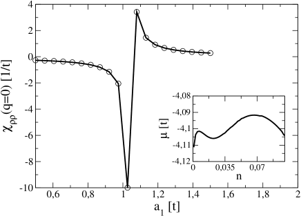
Figure 4: Main panel: $\chi_{\rho\rho}(q=0)$ vs. $a_{1}$ for $a_{0}=0.3$ and density $n=0.07$. A $q=0$ instability occurs at $a_{1}\approx 1.05$. Inset: The $\mu$ vs. $n$ curve for parameters $a_{0}=0.3$ and $a_{1}=1.05$ which demonstrates the zero slope at $n=0.07$.

Here the element $\chi_{\rho\rho}(q=0)$ is proportional to the compressibility, i.e. within our sign convention proportional to the inverse of $-\partial\mu/\partial n$. A (locally) stable system thus corresponds to $\chi_{\rho\rho}(q=0)<0$ whereas an unstable system is characterized by $\chi_{\rho\rho}(q=0)>0$.

Fig. 4 demonstrates the consistency of the present approach. For density $n=0.07$ and fixed $a_{0}=0.3$ the main panel shows $\chi_{\rho\rho}(q=0)$ as a function of $a_{1}$. Obviously the system changes from locally stable to locally unstable at $a_{1}\approx 1.05$. This is consistent with the $\mu$ vs. $n$ curve which is shown in the inset and shows a zero slope for the same parameters (cf. also upper left panel of Fig. 6).

Due to the momentum dependence of the density-current coupling and the momentum structure of $\chi^{0}(q)$ a finite $q$ instability can occur before. This is demonstrated in the left panel of Fig. 5 which shows the momentum dependence of $\chi_{\rho\rho}(q)$ along the $x$-direction. Clearly, as a function of $a_{1}$ a instability occurs at ${\bf q}\approx(0.3,0)$ before the ${\bf q}=0$ instability is reached. Moreover, the corresponding momentum is larger than one would expect from the nesting momentum of the upper band which is shown in the right panel of Fig. 5 which clearly reveals the importance of the momentum dependent coupling. A detailed investigation of the phase diagram and the corresponding structure of instabilities as a function of doping is presented in Ref. epl15ps, . In this latter work it was also shown that the Maxwell construction establishing the whole phase separated region preempts reaching the finite-$q$ instability

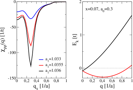
Figure 5: Left panel: $\chi_{\rho\rho}(q)$ vs. $(q_{x},0)$ for several $a_{1}$ ( momenta $q_{x}$ are in units of inverse of the lattice spacing $a$). Right panel: band structure along $(q_{x},0)$. Parameters: $a_{0}=0.3$ and density $n=0.07$.

III.2 Spin currents

Spin currents and associated torques are important quantities in characterizing the ground state of inhomogeneous Rashba models. In fact, the electron spin ${\bf S}$ is not a conserved quantity in systems with spin-orbit coupling. It obeys the Heisenberg equation of motion

$$\frac{d{\bf S}}{dt}=-\mathrm{i}[{\bf S},H]+\frac{\partial{\bf S}}{\partial t}$$ (8)

which can be interpreted in terms of a continuity equation

$${\bf G}=\mathrm{div}\,{\bf J}+\frac{\partial{\bf S}}{\partial t}$$ (9)

where ${\bf G}$ is a ’source’ term which in general is finite due to the non-conservation of spin. Since we are dealing with the time-independent Schrödinger equation where all expectation values are stationary, the source term is ’hidden’ in the commutator, i.e.

$$[{\bf S},H]=\mathrm{i}\,\mathrm{div}\,{\bf J}-\mathrm{i}{\bf G}$$ (10)

and ${\bf G}$ contains all contributions which cannot be associated with a divergence.

In particular one obtains for $J^{z}$ and $G^{x,y}$

$$J^{z}_{i,i+x(y)} = -\mathrm{i}\sum_{\sigma\sigma^{\prime}}\left[c^{\dagger}_{i\sigma}\tau^{z}_{\sigma\sigma^{\prime}}c_{i+x(y),\sigma^{\prime}}-c^{\dagger}_{i+x(y),\sigma}\tau^{z}_{\sigma^{\prime}\sigma}c_{i,\sigma}\right]$$

$$G_{i}^{x(y)} = \mathrm{i}\gamma_{i,i+x(y)}\times$$

$$\times \sum_{\sigma\sigma^{\prime}}\left[c_{n\sigma}^{\dagger}\tau^{z}_{\sigma\sigma^{\prime}}c_{i+x(y)\sigma^{\prime}}-c_{i+x(y)\sigma}^{\dagger}\tau^{z}_{\sigma\sigma^{\prime}}c_{i\sigma^{\prime}}\right]$$

corresponding to the relations

$$G_{i}^{x(y)}=-\gamma_{i,i+x(y)}J^{z}_{i,i+x(y)}-\gamma_{i-x(y),i}J^{z}_{i-x(y),i},$$ (11)

i.e., a torque for the $x(y)$-component of the spin is associated with a $z$-polarized spin current along the $x(y)$ direction when the RSOC $\gamma\neq 0$.

In a system with homogeneous RSOC one has finite $x(y)$-polarized spin currents flowing along the $y(x)$-direction. In particular, since the currents are constant the corresponding torques vanish and from Eq. (11) it turns out that $z$-polarized spin currents are absent in the homogeneous system. In the next subsection we demonstrate that the situation drastically changes when the RSOC depends on the density and thus induces an inhomogeneous charge distribution in the ground state.

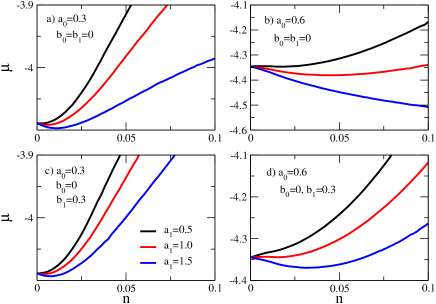
Figure 6: Chemical potential vs charge density for different parameters of the coupling constant. Each panel shows the curves for $a_{1}=0.5$ (black), $a_{1}=1.0$ (red), and $a_{1}=1.5$ (blue), whereas $a_{0}$ and $b_{1}$ are different in each panel.

IV Results for inhomogeneous charge and spin structures

In case of a homogeneous system Fig. 6 displays the chemical potential vs density for the various parameters entering the coupling constant Eq. (3). For simplicity only the case $b_{0}=0$ in Eq. (3) is considered. Clearly a phase separation instability is triggered by increasing the RSOC to the density via the parameter $a_{1}$. On the other hand the parameter $b_{1}$ puts an upper limit to this coupling so that the PS instability is shifted to lower doping upon increasing $b_{1}$.

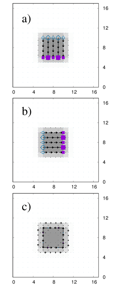
Figure 7: (a-c) The $x$- (panel a), $y$- (panel b), and $z$- (panel c) component of spin currents (arrows) and torques (circles, squares) for a phase separated solution. The distribution of charge ($26$ particles on a $16\times 16$ lattice) is indicated in grey. Parameters: $a_{0}=0.3$, $a_{1}=1.5$, $b_{0}=0$, $b_{1}=0$.

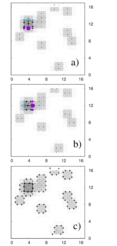
Figure 8: (a-c) The $x$- (panel a), $y-$ (panel b), and $z-$ (panel c) component of spin currents (arrows) and torques (circles, squares) for a phase separated solution including disorder $V_{0}/t=0.5$. The distribution of charge ($26$ particles on a $16\times 16$ lattice) is indicated in grey. Parameters: $a_{0}=0.3$, $a_{1}=1.5$, $b_{0}=0$, $b_{1}=0$.

Fig. 7 reports a particular realization of a phase-separated solution obtained on a $16\times 16$ lattice with $26$ particles. The charge carriers are confined to square shaped cluster with “large density sites” $n\approx 1$ and a border region with $n\approx 0.04$, indicated by dark and light grey squares, respectively. As in the homogeneous case the dominant flow of the $x(y)$-spin currents is along the $y(x)$ direction but now of course confined to the “large density square”. However, due to this confinement the currents are obviously not conserved but finite torques lead to a generation (annihilation) of spin currents. This implies finite torques $G^{x,y}$ for both $x$- and $y$- components at the border of the phase separated region which in turn from Eq. (11) induces $z$-polarized edge spin currents flowing counter clockwise around the square. Not that there is also a smaller edge current at the outer border (within the low density region) flowing clockwise. This is due to small $x(y)$-spin currents in this region (not visible on the scale of the plot) which flow opposite to the ones within the main square and thus are related to torques with opposite sign.

The pure phase separated state is very susceptible to the presence of disorder which will break up the system into “puddles” with enhanced charge density. This is shown in Fig. 8 for a disorder strength $V_{0}/t=0.5$. $x$- and $y$- polarized spin currents are dominant in the extended puddle with large charge density (around site $[4,12]$) but are also present (though not visible on the scale of the plot) in the smaller puddles. Again the most interesting observation is the torque induced flow of $z$-polarized spin edge currents around the puddles.

V Inhomogeneous Quantum Hall States

V.1 Momentum and real-space analysis of inhomogeneous QH states

Since a sufficiently strong and density dependent RSOC can promote an inhomogeneous electron state at LXO/STO interfaces, it is worthwhile investigating the properties of this inhomogeneous electron gas under a strong magnetic field $\mathbf{B}=B\hat{\bm{z}}$ perpendicular to the interface, in the quantum Hall regime. The Landau levels of a 2DEG in the presence of RSOC are rashba-qhe

$$E_{s}^{\pm}=\hbar\omega_{c}\left[s+\frac{1}{2}\pm\frac{1}{2}\mp\frac{\alpha}{\hbar}\sqrt{\frac{2m}{\hbar\omega_{c}}\left(s+\frac{1}{2}\pm\frac{1}{2}\right)}\,\right]$$

where $\omega_{c}=eB/m$ and we have taken the free-electron gyromagnetic factor $g=2$. As it is seen from the above equation, the RSOC $\alpha$ lifts the degeneracy of the levels $E^{+}_{s}$ and $E^{-}_{s+1}$ even at $g=2$, so all levels have the same degeneracy as the ground state and host the same number of states $N_{\phi}$. Furthermore, the level spacing is not constant and in particular the spacing between one level and the following with equal chirality decreases when the quantum number $s$ increases. The ordering of the levels is not defined a priori: the level $E^{+}_{s+1}$ may fall below the level $E^{-}_{s+1}$, provided the ratio $\alpha/\sqrt{B}$ is large enough. Only the level $E^{-}_{s=0}$ is independent of $\alpha$.

If the RSOC is constant, the chemical potential at $T=0$ is a non-decreasing step-wise function of the electron density, as in the case $\alpha=0$. However, if the RSOC depends on the electron density, $\mu$ may decrease when jumping from one Landau level to the next. Within the present continuum model we adopt a density dependent RSOC of the form

$$\alpha(n)=\frac{2a_{1}n}{(1+2b_{1}n)^{3}}$$ (12)

in agreement with Eq. (3) once the identification $n_{i}=n_{i+\eta}=n$ is adopted in the continuum limit, and, for simplicity, $a_{0}=b_{0}=0$. Furthermore, if the conditions required in Sec. II.2 are met, a situation like the one depicted in Fig. 9 occurs, where the stepwise function $\mu(n)$ oscillates around the smooth curve $\mu_{B=0}(n)$, which is itself a non-monotonic function of the density. Thus we may expect inhomogeneous quantum Hall states to occur.

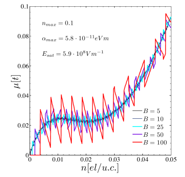
Figure 9: Chemical potential as a function of the electron densities at various magnetic fields. The values of the parameters ($a_{1}$ and $b_{1}$) determining the RSOC are such that the maximum value $\alpha_{max}$ reported in the figure panel is reached at a density $n_{max}$ (per unit cell). The maximum value $E_{max}$ of the interfacial electric field is also reported. The units of the magnetic field $B$ are in Tesla.

To investigate the properties of inhomogeneous quantum Hall states, we performed calculations in real space, with the Hamiltonian

$$\mathcal{H}=\sum_{i,\sigma}\left[t_{i,i+x}\left(\mathrm{e}^{\mathrm{i}By_{i}}c^{\dagger}_{i+x,\sigma}c_{i,\sigma}+h.c.\right)\right.$$

$$\left.+t_{i,i+y}\left(c^{\dagger}_{i+y,\sigma}c_{i,\sigma}+h.c.\right)+(B\sigma-\mu+\lambda_{i})c^{\dagger}_{i,\sigma}c_{i,\sigma}\right]$$

$$+\mathrm{i}\sum_{i,\sigma\sigma^{\prime}}\left[\gamma_{i,i+x}\left(\mathrm{e}^{-\mathrm{i}By_{i}}c^{\dagger}_{i,\sigma}\tau^{y}_{\sigma\sigma^{\prime}}c_{i+x,\sigma^{\prime}}+h.c.\right)\right.$$

$$\left.-\gamma_{i,i+y}\left(c^{\dagger}_{i,\sigma}\tau^{x}_{\sigma\sigma^{\prime}}c_{i+y,\sigma^{\prime}}+h.c.\right)\right]-\sum_{i}\lambda_{i}n_{i},$$

and the density dependent RSOC is described as before, by taking Eq. (3) with $a_{0}=b_{0}=0$. The results reported below are obtained for a square lattice of size $L=16$. In the absence of RSOC, the commensurability condition requires that the magnetic flux through a unit cell $\phi_{a}$ is a rational fraction $p/q$ of the flux quantum $\phi_{0}$. Under this condition, the size of the magnetic unit cells $1\times q$. Although for the chosen Landau gauge $\left[{\bf A}=(By,0,0)\right]$ the vector potential breaks the translational invariance along $y$, the system preserves the symmetry for translations of $q$ lattice spacings along $y$ (see, e.g., Ref. fradkin, ). Then, if the system is composed by an integer number of magnetic cells along $y$, periodic boundary conditions (PBCs) can be imposed. In a $16\times 16$ lattice, the lower field compatible with the latter condition corresponds to the ratio $p/q=1/16$, yielding $B_{min}=1692$ T, given the planar unit cell of LXO/STO. We notice in passing, that such a large unphysical magnetic field is only required to deal with a small enough cluster to be numerically manageable. Since the RSOC affects the QH states via the combination $\sqrt{\alpha^{2}/B}$, the same physics can be obtained by choosing a ten times smaller RSOC and a hundred times smaller field $B\sim 17$ T. This, however, gives rise to a ten times larger magnetic length, that would require larger real-space clusters. In order to attack this problem with real-space calculations, we are therefore led to use larger fields having in mind that the same physical effects would occur at much lower fields on somewhat larger length scales. For the case at hand, the resulting Hofstadter spectrum is composed of 16 sub-bands, each of them accommodating 16 electrons. If spin is taken into account the number of the sub-bands doubles. If $N=16$ electrons are present, the ground state corresponds to the complete filling of the first level. The electron density is homogeneous and a current locally flows along $x$, within the chosen gauge (see Fig. 10).

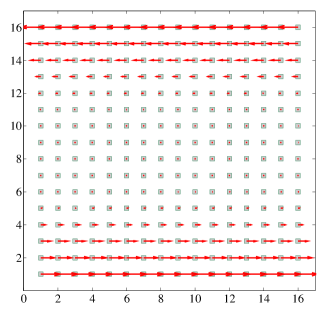
Figure 10: Charge density distribution and charge current for a $16\times 16$ system with $N=16$ electrons with PBCs. The lowest sub-band is completely filled.

The main features of quantum Hall states are deeply related to the existance of boundaries delimiting the physical space available for electron motion. When electrons are confined in a box, the wave functions must vanish approaching the walls. The effect of the boundaries is to lift the degeneracy of the Hofstadter sub-bands, that acquire a finite width. In other words, each sub-band in turn splits into a stack of levels. In Fig. 11 for pedagogical reasons and for the sake of comparison, we show the charge distribution and the edge currents for systems with $N=12$ (left) and $N=16$ (right) electrons, respectively, with open boundary conditions (OBCs). In the first case, all the electrons are accommodated in the lowest sub-band and a single edge current goes through the sample. The charge density is substantially homogeneous in the bulk and decreases when approaching the boundaries. For $N=16$, instead, the first sub-band is completely filled and the second one is partially filled, unlike the situation with PBCs where for $N=16$ the latter was empty. The second sub-band is characterized by a negative conductance and two different edge states with currents flowing in opposite directions are achieved (left panel). If no spin-orbit coupling is present, the $z$-spin current is simply opposite to the charge current: when the electrons move towards the left, there is a net spin current along the direction of their motion, while the electric current is directed to the right.

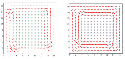
Figure 11: Homogeneous states of a for a $16\times 16$ system in the quantum Hall regime without RSOC, for OBCs. Left: The lowest sub-band only is populated. Right: Opposite edge currents due to the filling of different Hofstadter sub-bands.

When RSOC (and its dependence on the local density) is taken into account, our real-space numerical analysis automatically carries out a minimization of the ($\lambda$ constrained) energy, by allowing inhomogeneous solutions when phase separation occurs. In Fig. 12 we compare a situation in which the homogeneous system is inside the phase-separation region ($N=36$) and a system in which the homogeneous system is outside the phase-separation region ($N=101$). As it is evident, in the former case, we obtain an inhomogeneous solution in our real-space calculation. Interestingly, the edge currents run along the boundary of the self-nucleated droplet.

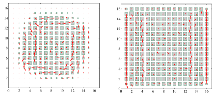
Figure 12: Charge density distributions and charge currents for a $16\times 16$ system. Left: Inhomogeneous quantum Hall state for a number of electrons $N=36$, corresponding to a filling at which the infinite homogeneous systems falls inside the phase-separation region. Right: Homogeneous quantum Hall state for a number of electrons $N=101$, corresponding to a filling at which the infinite homogeneous systems falls outside the phase-separation region.

V.2 Lattice model for QHE: Harper equation with RSOC

We consider a square lattice infinite in the $x$-direction and extended over $L$ unit cells (lattice constant $a=1$) in the $y$-direction. Electrons can hop between neighboring sites in the $xy$-plane and are subject to a strong homogeneous magnetic field $\mathbf{B}=B\hat{\bm{z}}$ generated by a site-dependent vector potential $\bm{A}(j)=(-By_{j},0,0)$. The tight-binding Hamiltonian in presence of RSOC is $H_{\rm TB}=H_{0}+H_{\rm RSOC}$ with

$$H_{0} = -\sum_{j}t_{j,j+x}\Big{[}e^{i2\pi\phi y_{j}}c^{\dagger}_{j+x}c_{j}+h.c.\Big{]}$$

$$- \sum_{j}t_{j,j+y}\Big{[}c^{\dagger}_{j+y}c_{j}+h.c.\Big{]}-E_{\rm Z}\sum_{j\sigma\sigma^{\prime}}\Big{[}c^{\dagger}_{j\sigma}\tau^{z}_{\sigma\sigma^{\prime}}c_{j\sigma^{\prime}}\Big{]},$$

$$H_{\rm RSOC} = \mathrm{i}\sum_{j,\sigma,\sigma^{\prime}}\gamma_{j,j+x}\Big{[}e^{i2\pi\phi y_{j}}c^{\dagger}_{j,\sigma}\tau^{y}_{\sigma\sigma^{\prime}}c_{j+x,\sigma^{\prime}}+h.c\Big{]}$$ (14)

$$- \mathrm{i}\sum_{j,\sigma,\sigma^{\prime}}\gamma_{j,j+y}\Big{[}c^{\dagger}_{j,\sigma}\tau^{x}_{\sigma\sigma^{\prime}}c_{j+y,\sigma^{\prime}}+h.c\Big{]}.$$

The orbital effect of the magnetic field is encoded in the phase factor acquired by the hopping amplitudes

$$t_{j,j+x(y)}\longrightarrow t_{j,j+x(y)}e^{\mathrm{i}e/\hbar\int_{j}^{j+x(y)}{\mathbf{A}\cdot\mathbf{dr}}},\,\,\,\,\,\,\,t_{j,j+x(y)}=t_{x(y)}$$

and

$$\gamma_{j,j+x(y)}\longrightarrow\gamma_{j,j+x(y)}e^{\mathrm{i}e/\hbar\int_{j}^{j+\hat{x}(\hat{y})}{\mathbf{A}\cdot\mathbf{dr}}},\,\,\,\,\,\,\gamma_{j,j+x(y)}=\gamma_{x(y)}$$

which can be written in terms of the flux $\phi$ through a lattice cell (in units of the flux quantum $\phi_{0}=h/e$). $\tau^{x}$, $\tau^{y}$ and $\tau^{z}$ are Pauli matrices acting on the electron spin and $E_{\rm Z}=g2\pi\phi$ the Zeeman coupling constant. An eigenstate of $H_{\rm TB}$ can be expanded as $|\Psi\rangle=\sum_{j\sigma}\psi_{\sigma}(x_{j},y_{j})c^{\dagger}_{j\sigma}|0\rangle$, with the wavefunction $\psi_{\sigma}(x_{j},y_{j})=\psi_{\sigma}(\ell,m)$ centered on the lattice site of coordinates $x_{j}=\ell$ and $y_{j}=m$. Translational invariance along $x$ allows for the factorization $\psi_{\sigma}(\ell,m)=\psi_{\sigma}(m)e^{ik_{x}\ell}$ and the eigenvalue problem can be solved in a ribbon of vertical size $L$.

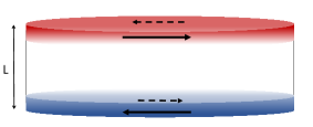
Figure 13: Schematic view of a ribbon with periodic boundary conditions along $x$ and finite size $L$ along $y$. For an homogeneous state only two edge states are present: the upper edge state (red) flows counterclockwise, while the lower edge (blue) flows clockwise.

The Schrödinger equation for the spinor

$$\Psi_{m}=\left(\begin{aligned} &\psi_{m\uparrow}\\ &\psi_{m\downarrow}\end{aligned}\right)\,\,\,\,\,m=0,\cdots,L-1$$ (15)

reads as

$$E\Psi_{m}=D_{m}\Psi_{m}+R_{m}\Psi_{m+1}+R_{m}^{\dagger}\Psi_{m-1},$$ (16)

known as Harper equation hofstadter-1976 ; demikhovskii-2006 ; morais-smith-2012 . RSOC enters in the off-diagonal elements of the $2\times 2$ blocks

$$D_{m} =\begin{pmatrix}-2t_{x}\cos(\tilde{k}_{x})-E_{\rm Z}&2\mathrm{i}\gamma_{x}\sin(\tilde{k}_{x})\\ -2\mathrm{i}\gamma_{x}\sin(\tilde{k}_{x})&-2t_{x}\cos(\tilde{k}_{x})+E_{\rm Z}\end{pmatrix}$$

$$R_{m} =\begin{pmatrix}-t_{y}&\ -\mathrm{i}\gamma_{y}\\ -\mathrm{i}\gamma_{y}&-t_{y}\\ \end{pmatrix},$$

where $\tilde{k}_{x}\equiv k_{x}+2\pi\phi m$. The solution of the coupled eigenvalue equations defined by Eq. (16) returns $2L$ energy sub-bands $E_{\ell}(k_{x})$ with $\ell=0,1,\cdots,2L-1$. It is convenient to take the origin of the $y$-axis $m=0$ at the middle of the ribbon, so that $m$ takes the integer values between $-L/2$ and $L/2-1$ (for simplicity we assume $L$ to be even here).

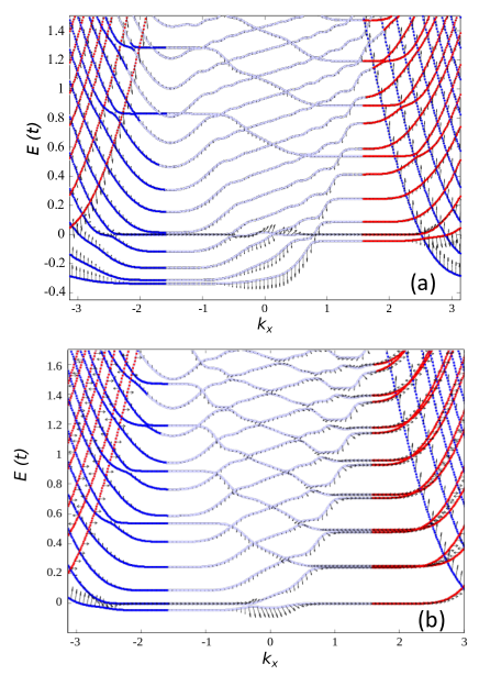
Figure 14: Electronic sub-bands for the two-dimensional system in strong magnetic field for (a) heterostructure formed by a region with RSOC ($\gamma_{1}=a_{01}=0.3t$ and a region with RSOC $\gamma_{2}=a_{02}=0.6t$; (b) heterostructure formed by a region without RSOC ($\gamma_{1}=0$ and a region with RSOC $\gamma_{2}=a_{0}=0.3t$. Colors distinguish the edge states – propagating along the top edge from left to right (in red) and along the bottom edge from right to left (in blue) – from the bulk states (light grey), according to the calculated expectation value of the $y$-coordinate $\langle m\rangle=\sum_{m\sigma}m|\psi_{m\sigma}|^{2}$. Black arrows represent magnitude and direction of the expectation value of the spin angular-momentum: vertical arrows stay for $\langle\sigma_{y}\rangle=1,\,\langle\sigma_{z}\rangle=0$, horizontal arrows for $\langle\sigma_{y}\rangle=0,\,\langle\sigma_{z}\rangle=1$.

In order to investigate inhomogeneous quantum Hall states we consider an interface in the $y$-direction between two (macroscopic) regions with different RSOC $\gamma_{1}$ and $\gamma_{2}$ (which might result from different electronic densities in the two regions due to a density-dependence of the RSOC) and compare the spectrum – as a function of the momentum $k_{x}$ – for this heterostructure with the conventional spectrum of Landau levels in absence of RSOC and with the case where RSOC is present but is homogeneous. Given a ribbon as in Fig. 13, numerical results are shown in Fig. 14 for the different cases: (a) $\gamma_{y(x)}=\gamma_{1}=0.3t$ for $0<m\leq L/2-1$, $\gamma_{y(x)}=\gamma_{2}=0.6t$ for $0>m\geq-L/2$ and $\gamma_{y}=(\gamma_{1}+\gamma_{2})/2$ at $m=0$; (b) $\gamma_{y(x)}=\gamma_{1}=0$ for $0<m\leq L/2-1$, $\gamma_{y(x)}=\gamma_{2}=0.3t$ for $0>m\geq-L/2$ and $\gamma_{y}=(\gamma_{1}+\gamma_{2})/2$ at $m=0$.

At $\phi\ll 1$ the bulk spectrum consists of a set of flat bands (Landau levels) which have different ordering and spin-polarizations depending on whether RSOC is present or not. Of course, inhomogeneous QH states have been investigated before (see, e.g., Ref. venturelli-2011, ; champel-2013, ; hashimoto-2008, ; lado-2013, and references therein). However, it is interesting that we face here an inhomogeneous QH state where different strengths of the local RSOC induce differently spin-polarized edge states. In Fig. 14(a,b) one can distinguish two sets of bulk levels which are connected at $k_{x}\approx 0$. It is interesting to note the avoided crossings between levels with different quantum numbers and the variation of the orientation of the spin particularly along the lowest energy levels. On the one hand, case (a) is rather similar to the case of no RSOC and differently gated regions of the system that was considered in Ref. venturelli-2011, . The main difference here is that the presence of a sizable RSOC forces the spin polarization of the edge states (moving in the $x$ direction) along the $y$ direction instead of the usual $z$ direction. On the other hand, in the case of Fig. 14(b) the upper edge lives in a region of vanishing RSOC and is polarized along $z$, while the blue (i.e. lower) edge lives in a region of sizable RSOC and carries a chiral spin polarized along $y$. The corresponding edge states that mix and interfere inside the bulk of the ribbon give rise to smoothly rotating spin polarizations. These effects, might be of applicative relevance for spin interferometry.giovannetti-2012 or they might play important roles in electronic transport. Note that even at $\gamma\neq 0$ there is always a level with electrons having the spin polarized in the $z$-direction, regardless of the momentum $k_{x}$ (the $s=0$ level in the previous section).

VI Spin Hall effect

In the ground state of the Rashba model the total $x(y)$-torques have to vanish and therefore from Eq. (11) we get

$$\sum_{i}G_{i}^{x(y)}=0=-\gamma_{i,i+x(y)}J^{z}_{i,i+x(y)}-\gamma_{i-x(y),i}J^{z}_{i-x(y),i},$$ (17)

which implies also a vanishing of the total $z$-polarized spin currents for $\gamma_{i,i+x(y)}=const$. However, consider for example a system with striped RSOC as depicted in the inset to Fig. 15b. Denote with $J^{z}_{1,2}$ the total z-spin current flowing along the bonds of the $\gamma_{1,2}$-stripes which are assumed to have the same width. Then we can rewrite Eq. (17) as

$$0=\gamma_{1}J^{z}_{1}+\gamma_{2}J^{z}_{2}\,\,\longrightarrow\,\,J^{z}_{2}=-\frac{a_{1}}{a_{2}}J^{z}_{1}$$

and the total $z$-spin current of the system is thus given by

$$J^{z}_{tot}=n_{str}\left(J^{z}_{1}+J^{z}_{2}\right)=n_{str}J^{z}_{1}\left(1-\frac{\gamma_{1}}{\gamma_{2}}\right)\,,$$

where $n_{str}$ denotes the total number of $\gamma_{1,2}$ stripes.

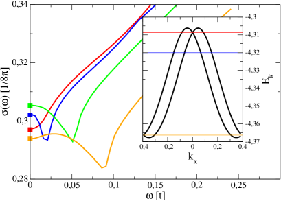
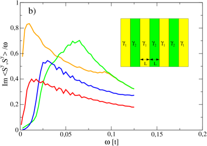
Figure 15: Top panel: Frequency dependence of the spin Hall correlation function Eq. (18) for different values of the chemical potential which is located within the lowest bands as indicated in the inset. Lower panel: Imaginary part of the response related to the time derivative of $S^{y}$. The inset depicts the coupling structure of the striped Rashba system ($L=4$) with RSOC $\gamma_{1}=0.2t$ and $\gamma_{1}=0.8t$, respectively.

The same reasoning can also be applied in a non-equilibrium situation, i.e. in the presence of an applied electric field, where it gives rise to the so-called spin Hall effect (SHE) dyakonov1971 , i.e. the generation of a transverse spin current by an applied electric field with the current spin polarization being perpendicular to both the field and the current flow. For a homogeneous system (with homogeneous linear RSOC) the SHE vanishes in a stationary situation because of the same argument, which leads to Eq. (17) and which has been first pointed out by Dimitrova dimitrova05 . On the other hand we have shown in Refs. epl, ; jscmag, ; jmagmat, that in the linear response regime a periodic modulation of the RSOC as depicted in Fig. 15 generates a finite SHE within the low doping doping regime where the electronic states are localized but can sustain a finite spin current under stationary conditions.

The spin Hall coefficient can be obtained as the zero frequency limit of the following spin-charge current correlation function as

$$\sigma^{sH}(\omega) = \sum_{ij}\Re\sigma^{reg}_{ij}(\omega)$$ (18)

$$\sigma^{reg}_{ij}(\omega) = -\frac{\mathrm{i}e}{N}\sum_{\ell,m}\frac{f_{\ell}-f_{m}}{E_{\ell}-E_{m}}\frac{\langle\ell|j^{z}_{i,i+y}|m\rangle\langle m|j^{ch}_{j,j+x}|\ell\rangle}{\omega+\mathrm{i}\eta+E_{\ell}-E_{m}},\,$$

where $|\ell\rangle$ and $E_{\ell}$ are exact eigenstates and eigenvalues of the system and $f_{\ell}$ denotes the corresponding Fermi function. Due to the modulation of the RSOC, there a band folding producing a sub-band structure in the reduced Brillouin zone. Fig. 15a shows the frequency dependence of $\sigma^{sH}(\omega)$ for a $L=4$ striped system (cf. inset to panel b) and a set of chemical potentials within the lowest pair of Rashba split sub-bands. Clearly $\sigma^{sH}(\omega)$ approaches a finite value for $\omega\to 0$ which is slightly reduced when the chemical potential corresponds to the energy of a band crossing. However, one has to additionally show that this is a result obtained under stationary conditions. This can be substantiated from the computation of $\Im\chi(S^{y},S^{y})/\omega$ which corresponds to the dynamics of the time derivative of $S^{y}$. From Fig. 15b it turns out this quantity vanishes in the limit of $\omega\to 0$ due to the strong localization of the bands perpendicular to the stripe direction. The vanishing of $dS^{y}/dt$ can also be derived directly from the equation of motion for $S^{y}$ which then provides another validation for Eq. (17) epl .

It is important to note that this effect is due to the modulation of the RSOC and cannot arise in a conventional charge-density wave system. Experimentally our proposal could be realized in the 2DEG at the interface of a LaAlO₃/SrTiO₃ ( LAO/STO) heterostructure with periodic top gating or in heterostructures of semiconductors with modulated Rashba SOC which have been already discussed in the literature in different contexts wang04 ; japa09 ; malard11 .

VII Conclusions

In this paper we discuss the role of density inhomogeneities in oxide interfaces. These inhomogeneities seem to be a common (if not ubiquitous) occurrence in LXO/STO oxide interfaces and likely have a submicrometric character. The inhomogeneous density distribution is directly related to an inhomogeneous distribution of the confining electric field perpendicular to the interface and, in turn, to an inhomogeneous distribution of the RSOC. This naturally leads to the idea that the RSOC can be phenomenologically assumed as a function of the local density, that increases at low density and is implemented in the simplified model presented in Sect. III. The RPA analysis and the real-space solution of the model on finite clusters show that a phase-separation instability is present, which also preemps the occurrence of an electronic instability at finite momentum.

The explicit solution of the model in real space finite lattices directly shows that the density-driven RSOC can indeed induce (or at least makes it easier) an EPS and that the high-density phase is fragmented into ‘puddles’ when disorder is present. This inhomogeneous distribution of electrons and RSOC gives rise to spin torques at the puddle boundaries. These torques act as sources and drains of spin currents, which tend to flow inside and around the puddles.

Spin and charge currents also flow at the boundaries of the density inhomogeneities, when strong magnetic fields drive the system into a quantum Hall state. When the edge is between a metallic filled region and an empty insulating matrix, the edge state assumes a simpler structure with the RSOC linking the spin to the momentum inducing a chiral edge state with the spin polarization on the interface plane. The edge states are instead more intricate and display a complex behavior at the interface between regions with differently filled Landau levels.

In summary, electronic inhomogeneities in oxide interfaces can induce inhomogeneous RSOC leading to interesting new physical effects (inhomogeneous spin currents and edge states). Of course these effects can be exploited and engineered for applicative purposes. This paves the way to effects of interest for spintronics, like spin interferometry or the occurrence of a robust spin Hall effect in systems with striped RSOC.

Acknowledgments

The Authors gratefully thank L. Benfatto and C. Castellani for stimulating discussions. This work was financially supported by the Ateneo 2016 project ‘Superconductivity in soft electronic matter’ of the University of Rome ‘Sapienza’

References

- (1) A. Ohtomo and H. Y. Hwang, (2004) Nature 427, 6
- (2) N. Reyren, et al., (2007) Science 317, 1196
- (3) A. Caviglia, et al., (2008) Nature 456, 624
- (4) J. Biscaras et al., (2010) Nat. Commun. 1, 89
- (5) J. Biscaras, et al., (2012) Phys. Rev. Lett. 108, 247004
- (6) Ariando, et al., (2011) Nat. Commun. 2, 188
- (7) Li Lu, C. Richter, J. Mannhart, and R. C. Ashoori, (2011) Nat. Phys. 7, 762
- (8) J. A. Bert et al., (2011) Nat. Phys. 7, 767
- (9) D. A. Dikin, et al., (2011) Phys. Rev. Lett. 107, 056802
- (10) M. M. Mehta, et al., (2012) Nat. Commun. 3, 955
- (11) J. A. Bert , et al., (2012) Phys. Rev. B 86, 060503(R)
- (12) G. E. D. K. Prawiroatmodjo, et al. (2016), Phys. Rev. B 93 184504.
- (13) A. D. Caviglia, et al., (2010) Phys. Rev. Lett. 104, 126803
- (14) M. Ben Shalom, et al., (2010) Phys. Rev. Lett. 105, 206401.
- (15) S. Caprara, F. Peronaci, and M. Grilli, (2012), Phys. Rev. Lett. 109, 196401
- (16) S. Hurand, et al., (2015), Sci. Rep. 5 12751.
- (17) Y. A. Bychkov and E. I. Rashba, (1984), J. Phys. C 17 6039
- (18) C. Bell, et al. (2009), Phys. Rev. Lett. 103, 226802
- (19) S. Caprara, M. Grilli, L. Benfatto, and C. Castellani (2011), Phys. Rev. B 84, 014514
- (20) D. Bucheli, S. Caprara, C. Castellani, and M. Grilli (2013), New J. Phys. 15 023014
- (21) Z. Ristic Z, et al. (2011) Europhys. Lett. 93, 17004
- (22) Feng Bi et al. (2013) arXiv:1302:0204
- (23) D. Bucheli, S. Caprara, and M. Grilli, (2015) Supercond. Sci. Technol. 28, 045004
- (24) C. Richter et al. (2013) Nature 502 528
- (25) Beena Kalisky, et al., (2013) Nat. Mat. 12 1091
- (26) M. Honig, J. A. Sulpizio, J. Drori, A. Joshua, E. Zeldov and S. Ilani, (2013) Nat. Mat. 12 1112
- (27) S. Caprara et al. (2013) Phys. Rev. B 88 020504(R).
- (28) S. Caprara, et al., (2015) Supercond. Sci. Technol. 28 014002
- (29) J. Biscaras et al., (2013) Nat. Mater. 12 542
- (30) D. Stornaiuolo,et al., (2012) App. Phys. Lett. 101, 222601
- (31) Uwe Treske, Nadine Heming, Martin Knupfer, Bernd Büchner, Emiliano Di Gennaro, Amit Khare, Umberto Scotti Di Uccio, Fabio Miletto Granozio, Stefan Krause, and Andreas Koitzsch, Universal electronic structure of polar oxide hetero-interfaces, Sci. Rep. in press.
- (32) M. Salluzzo, J. C. Cezar, N. B. Brookes, V. Bisogni, G. M. De Luca, C. Richter, S. Thiel, J. Mannhart, M. Huijben, A. Brinkman, G. Rijnders, and G. Ghiringhelli, (2009) Phys. Rev. Lett. 102, 166804.
- (33) Z. Zhong, A. Töth, and K. Held, (2013) Phys. Rev. B 87, 161102(R).
- (34) Z. Popovic̀, S. Satpathy, and R. Martin, (2008) Phys. Rev. Lett. 101, 256801
- (35) P. Delugas, A. Filippetti, V. Fiorentini, D. I. Bilc, D. Fontaine, and Ph. Ghosez (2011) Phys. Rev. Lett. 106 166807
- (36) N. Nakagawa, H. Y. Hwang, and D. A. Muller, (2006) Nat. Mater. 5 204.
- (37) Liping Yu and Alex Zunger, (2014) Nat. Commun. 5, 5118
- (38) D. Bucheli, M. Grilli, F. Peronaci, G. Seibold, and S. Caprara, (2014) Phys. Rev. B 89, 195448
- (39) N. Scopigno et al., (2016) Phys. Rev. Lett. 116, 026804
- (40) E. Fradkin, Field Theories of Condensed Matter systems, Addison-Wesley Publishing Company, 1991.
- (41) M. I. Dyakonov and V. I. Perel, (1971) Phys. Lett. A 35, 459
- (42) G. Seibold, D. Bucheli, S. Caprara, and M. Grilli, (2015) EPL 109, 17006.
- (43) Ol’ga V. Dimitrova, (2005) Phys. Rev. B 71, 245327.
- (44) G. Seibold, S. Caprara, M. Grilli, and R. Raimondi, (2015) EPL 112, 17004.
- (45) G. Seibold, S. Caprara, M. Grilli, and R. Raimondi, (2017) Journal of Superconductivity and Novel Magnetism 30, 123.
- (46) G. Seibold, S. Caprara, M. Grilli, and R. Raimondi, (2017) Journal of Magnetism and Magnetic Materials, http://dx.doi.org/10.1016/j.jmmm.2016.12.066.
- (47) X. F. Wang, (2004) Phys. Rev. B 69, 035302 .
- (48) G. I. Japaridze, Henrik Johannesson, and Alvaro Ferraz, (2009) Phys. Rev. B 80, 041308(R).
- (49) Mariana Malard, Inna Grusha, G. I. Japaridze, and Henrik Johannesson, (2011) Phys. Rev. B 84, 075466.
- (50) E. I. Rashba, (1960) Fiz. Tverd. Tela (Leningrad) 2, 1224. [E. I. Rashba, (1960) Sov. Phys.-Solid State 2 1109]
- (51) D. R. Hofstadter, (1976) Phys. Rev. B 14, 2239.
- (52) V. Ya. Demikhovskii and A. A. Perov, (2006) Europhys. Lett., 76, 477
- (53) W. Beugeling, N. Goldman, and C. Morais Smith, (2012) Phys. Rev. B 86, 075118
- (54) D. Venturelli et al., (2011) Phys. Rev. B 83, 075315.
- (55) Daniel Hernangómez-Pérez, et al., (2013) Phys. Rev. B 88, 245433
- (56) K. Hashimoto, et al., (2008) Phys. Rev. Lett. 101, 256802.
- (57) J. L. Lado, et al., (2013) Phys. Rev. B 88, 035448.
- (58) Luca Chirolli, Davide Venturelli, Fabio Taddei, Rosario Fazio, and Vittorio Giovannetti, (2012) Phys. Rev. B 85, 155317