Influence of anisotropic surface roughness on lubricated rubber friction with application to hydraulic seals

Abstract

Machine elements and mechanical components have often surfaces with anisotropic roughness, which may result from the machining processes, e.g. grinding, or from wear. Hence, it is important to understand how surface roughness anisotropy affects contact mechanics properties, such as friction and the interface separation, which is important for lubricated contacts. Here we extend and apply a multiscale mean-field model to the lubricated contact between a soft (e.g. rubber) elastic solid and a rigid countersurface. We consider surfaces with anisotropic surface roughness, and discuss how the fluid flow factors and friction factors depend on the roughness. We present an experimental study of the lubricated sliding contact between a nitrile butadiene rubber O-ring and steel surfaces with different types of isotropic and anisotropic surface roughness. The good quantitative comparison between the experimental results and the theory predictions suggests that the multiscale lubrication mechanisms are accurately captured by the theory.

1 Introduction

Soft contacts are crucial in numerous engineering and biological applications, and have gained increasing attention by scientists working in fundamental sciencegeneral_multiscale ; Ma20157366 ; 10.1371/journal.pone.0143415 and computational mechanicsStupkiewicz2016511 . Soft contacts occur, e.g., in the tribology of machine elementsSalant1999189 ; Hajjam200413 ; Wohlers200951 ; Scaraggi2012 ; Tan2015236 ; Scaraggi2014118 , in living matterDunn201345 ; Khosla201517587 ; Greene20115255 , and medical devicesLorenz2013 ; Sterner2016 , to name just a few. In some specific applications, the wet grip performance becomes the subject of international regulation, such as for tires (e.g. the EU tire label directiveEU.tires ) and for personal protective shoes (see e.g the test method for slip resistance of footwear ISO 13287:2012, leading to the GRIP rating documents by the Health & Safety Laboratory HSL, UK). In some other applications, instead, different surface roughness descriptors become the key parameters to be associated with the device failure behavior, such as the International Roughness Index (IRI) for road pavement engineering (shown to be related to the vehicles crash-ratepavement ) or a set of shaft roughness descriptors for rotatory sealsFlitney (to be kept within an allowable range of values, see e.g. RMA OS-1-1 and ISO 6194-1:2009).

Interestingly, despite the social, economic and environmental relevancy of the applications described above, the underlying tribological nature of the generic soft contact has not been widely recognized. Consequently, a strongly diverse design approach, often of the try-and-error nature, is used in those apparently-different (but fundamentally similar) scientific and technological fields. This might suggest that a dedicated applied research is probably needed to inject the current theoretical tribology understanding to practical applications of soft contacts.

A soft contact typically refers to an interaction between solids where at least one of the solids is characterized by a relatively small elastic modulus (say in the range $\mathrm{kPa}$ to $\mathrm{MPa}$). This results in relative low contact pressures (typically $\sim 1\ \mathrm{MPa}$ or less) which imply that the fluid rheology can be treated as pressure independent, i.e., the classical “high” pressure lubricant behaviors, such as piezo-viscosity and piezo-density, are unimportant. However, depending on the contact conditions other complex phenomena may appears such as the dewetting transitions (regulated by the interface spreading pressure). On the theoretical side, the fundamental understanding of the key role of roughness in soft interface mechanics, at least in those cases where adhesion/capillary, hydration and weeping mechanisms can be neglected, has been the subject of numerous investigations, in particular about the multiscale description of real surfaces under dry Persson20013840 ; Carbone2009 ; general_multiscale and wet BP ; Scaraggi2014118 ; Scaraggi2012 ; MS1 ; MS2 ; MS3 ; MS4 ; MS5 ; MS6 conditions. In Refs. BP ; MS2 ; MS4 Persson, Scaraggi et al. have derived a mean-field theory of the thin film lubrication, characterized by the so called flow and shear stress factorsPatir197812 . The theory can be applied to the lubricated contact between soft solids with realistic surface roughness, for both Newtonian and non-Newtonian fluids, and for anisotropic roughness.

In this work we will extend and apply the theory MS2 to practical cases, trying to unravel how specific anisotropy roughness parameters affect the so-called flow and stress factors which enter the fluid flow equation and the expression for the frictional shear stress. A case study related to dynamic seals with line contact geometry, such as O-rings, will be reported, together with an experimental study. Indeed, among the others, seals are crucial machine elements in almost any mechatronic device, and in particular in hydraulic and pneumatic components, where a seal failure can result in expensive production downtime or even environmentally hazardous leakage.

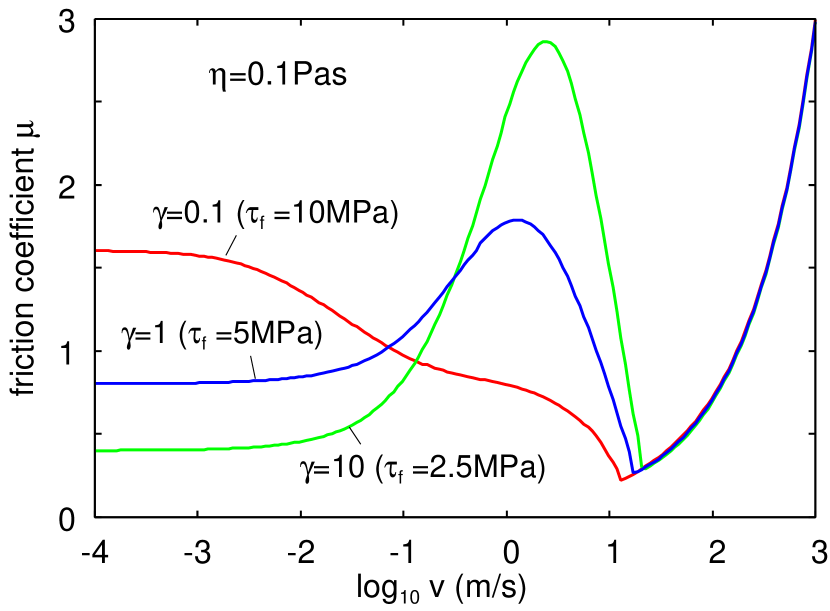
Figure 1: The calculated friction coefficient (Stribeck curves) as a function of the logarithm of the sliding speed for three different surfaces with the same angular averaged power spectra but different surface asymmetry. For a rubber cylinder (radius $R=2.5\ {\rm mm}$) with the normal load per unit length $F_{\rm N}/L=200\ {\rm N/m}$, sliding in the $x$-direction, orthogonal to the cylinder axis ($y$-direction). The substrate surface is rigid and randomly rough with the Tripp numbers: $\gamma=1$ (isotropic roughness), $\gamma=10$ (scratches along the sliding direction), and $\gamma=0.1$ (scratches orthogonal to the sliding direction). The rubber elastic modulus $E=5\ {\rm MPa}$ and Poisson ratio $\nu=0.5$. The lubricant fluid is Newtonian with the viscosity $\eta=0.1\ {\rm Pas}$. We assume in the area of real contact occur a frictional shear stress which equal $\tau_{\rm f}=10$, $5$ and $2.5\ {\rm MPa}$ for $\gamma=0.1$, $1$ and $10$, respectively. The substrate surfaces have the root-mean-square (rms) roughness $h_{\rm rms}=10\ {\rm\mu m}$, the rms slope 1.5 and the Hurst exponent $H=0.8$.

Surface roughness anisotropy can have different influence on the friction coefficient (and on wear) depending on the sliding speed. To illustrate this, consider a rubber cylinder sliding orthogonal to the cylinder axis on a lubricated substrate. The substrate is rigid and we consider two cases where the substrate has roughness scratches orthogonal to the sliding direction i.e. along the cylinder axis (corresponding to the Tripp number $\gamma<1$), and when the scratches are along the sliding direction (corresponding to the Tripp number $\gamma>1$). We assume the same angular averaged surface roughness power spectra in both cases.

In the boundary lubrication velocity region the friction force will be highest when the scratches are orthogonal to the sliding direction since in this case the rubber will be exposed to stronger time dependent deformations by the substrate asperities, resulting in a large viscoelastic contribution to the friction. For dry surfaces this has indeed been observed in experimentsCarbone2009 .

In the high-velocity part of the mixed lubrication region of the Stribeck curve the situation is opposite to that in the boundary lubrication regime. Thus when the scratches are orthogonal to the sliding direction, fluid in the valley cannot escape from the nominal rubber-substrate contact region as easily as when the scratches are along. This results in a stronger hydrodynamic pressure buildup, and larger surface separation, and lower friction force. This is illustrated in Fig. 1 where we show the calculated Stribeck curves (using the theory developed in Ref. MS2 ) for three surfaces with identical angular averaged surface roughness power spectra, but different anisotropy: $\gamma=1$ (isotropic roughness), $\gamma=0.1$ (scratches along the cylinder axis, orthogonal to the sliding direction) and $\gamma=10$ (scratches along the sliding direction).

The paper is organized as following. In Sec. 2 we provide a summary of the mean field theory for lubrication, with emphasis on the theory of flow and shear stress factors for the specific contact conditions matching the experimental setup. Furthermore we present numerical results which illustrate how different roughness parameters affect the flow and friction factors, and the related friction curves. In Sec. 3 we describe the experimental apparatus built for the friction tests, and in Sec. 4 we present the surface roughness power spectra of the studied surfaces. Sec. 5 reports the friction measurements. The measured data are compared in detail to theory predictions in Sec. 6. Sec. 7 contains the summary and conclusions.

2 Mean field theory of lubrication

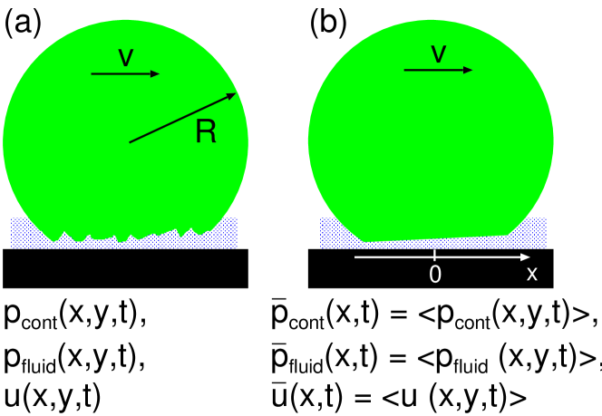
Figure 2: (a) Schematic of a rubber ball with a rough surface sliding on a smooth rigid substrate surface. Physical quantities like the contact pressure, the fluid pressure and the interface separation varies rapidly in space over many decades in length scales due to the nature of the surface roughness. The complex situation in (a) can be mapped on a simpler situation (b) where the fluid and contact pressures, and the surface separation, are locally-averaged quantities, which vary slowly in space on the length scale of the surface roughness. Those averaged quantities obey to modified fluid flow equations which contain two functions, denoted as flow factors, which depend on the locally averaged surface separation, and which are mainly determined by the surface roughness.

2.1 Effective equations of motion

We consider the simplest problem of an elastic cylinder (upper solid with length $B$ and radius $R$, with $B>>R$) sliding on a rigid solid (lower solid) with a nominal flat surface. We consider two cases:

(A) The upper solid has surface roughness while the lower solid is perfectly smooth.

(B) The upper solid is perfectly smooth while the lower solid has surface roughness.

We assume that the sliding occurs in the direction perpendicular to the cylinder axis, and we introduce a coordinate system with the $x$-axis along the sliding direction and with $x=0$ corresponding to the cylinder axis position, see the schematic of Fig. 2. The cylinder is squeezed against the substrate by the normal force $F_{\mathrm{N}}$. In the contact region between the cylinder and the substrate acts a nominal contact pressure:

$$\bar{p}_{0}(x,t)=\bar{p}_{\mathrm{cont}}(x,t)+\bar{p}_{\mathrm{fluid}}(x,t),$$

where $\bar{p}_{\mathrm{cont}}$ and $\bar{p}_{\mathrm{fluid}}$ are, respectively, the mean field pressures due to the direct asperity- and fluid-asperity interactions. Note that $\bar{p}_{0}(x,t)$ is the microscopic pressure averaged over surface areas $\sim\lambda\times\lambda$, where $\lambda$ is the wavelength of the longest (relevant) surface roughness component. This approach assumes a separation of length scales so that $\lambda<<w$, where $w$ is the width of the nominal contact region (which is of order the Hertz’s contact length $a_{\mathrm{H}}$). We consider the case of constant normal load so that

$$\int_{-\infty}^{\infty}dx\ \bar{p}_{0}(x,t)={\frac{F_{\mathrm{N}}}{B}}.$$

Let $\bar{u}(x,t)$ denote the (locally averaged) separation between the surfaces. For $\bar{u}>h_{\mathrm{rms}}$, where $h_{\mathrm{rms}}$ is the root-mean-square (rms) roughness,

$$\bar{p}_{\mathrm{cont}}(x,t)\approx\beta E_{\mathrm{r}}\mathrm{exp}\left(-\alpha{\frac{\bar{u}(x,t)}{h_{\mathrm{rms}}}}\right),$$

where $\alpha$ and $\beta$ are described in Ref. Persson2007 . Eq. (3) is valid for large enough $\bar{u}$. Since an infinite high pressure is necessary in order to squeeze the solids into complete contact we must have $\bar{p}_{\mathrm{cont}}\rightarrow\infty$ as $\bar{u}\rightarrow 0$. This is, of course, not obeyed by (3), and in the following calculations we therefore use the numerically calculated relation $\bar{p}_{\mathrm{cont}}(\bar{u})$, the latter reducing to (3) for large enough $\bar{u}$.

The macroscopic gap equation is determined by simple geometrical considerations. Thus, assuming the cylinder deformation to be within the Hertz regime for elastic solids, the gap equation reads

$$\bar{u}(x,t)=\bar{u}_{0}(t)+{\frac{x^{2}}{2R}}-{\frac{2}{\pi E_{\mathrm{r}}}}\int_{-\infty}^{\infty}dx^{\prime}\ \bar{p}_{0}(x^{\prime},t)\mathrm{ln}\left|{\frac{x-x^{\prime}}{x^{\prime}}}\right|,$$

where in the most general line-contact case $1/R=1/R^{\mathrm{up}}+1/R^{\mathrm{low}}$, where $R^{\mathrm{up}}$ and $R^{\mathrm{low}}$ are the radius of curvature of the top and bottom surface, respectively. In (3) and (4) $1/E_{\mathrm{r}}=1/E_{\mathrm{r}}^{\mathrm{up}}+1/E_{\mathrm{r}}^{\mathrm{low}}$ in the most general case, where the reduced elastic modulus is defined by $E_{\mathrm{r}}=E/\left(1-\nu^{2}\right)$, with $E$ and $\nu$ the Young’s elastic modulus and the Poisson ratio, respectively. In addition, the pressure $\bar{p}_{0}(x,t)$ must satisfy the normal load conservation condition (2).

To complete the system of equations we need an equation which determine the fluid pressure $\bar{p}_{\mathrm{fluid}}(x,t)$. The fluid flow is determined by the Navier-Stokes equation, but in the present case of fluid flow in a narrow gap between the solid walls, this equation can be simplified under the so called lubrication approximation, leading to the Reynolds equation. For surfaces with roughness on many length scales, this equation (even reproducing only the laminar motion), when coupled with (4), is numerically too complex to be solved directly in most cases. However, when there is a separation of length scales, i.e., if the longest (relevant) surface roughness component has a wavelength much smaller than the nominal cylinder-countersurface contact length (in the sliding direction), then it is possible to eliminate or (in the language of the renormalization group theory) integrate out the surface roughness degrees of freedom and obtain an effective equation of motion for the (locally averaged) fluid pressure. Such equations are characterized by two correction factors, namely $\phi_{\mathrm{p}}$ (pressure flow factor) and $\phi_{\mathrm{s}}$ (shear flow factor), which are mainly determined by the surface roughness and depend on the locally averaged surface separation $\bar{u}$. Thus, the effective two-dimensional (2D) fluid flow current for the case A (stationary cylinder with roughness)MS2 :

$$\mathbf{J}=-{\frac{\bar{u}^{3}\phi_{\mathrm{p}}(\bar{u})}{12\eta}}\nabla\bar{p}_{\mathrm{fluid}}+{\frac{1}{2}}\bar{u}\mathbf{v}_{0}+{\frac{1}{2}}h_{\mathrm{rms}}\phi_{\mathrm{s}}(\bar{u})\mathbf{v}_{0}$$

satisfies the mass conservation equation

$${\frac{\partial\bar{u}}{\partial t}}+\nabla\cdot\mathbf{J}=0$$

Substituting (5) in (6), and assuming $\mathbf{v}=v_{0}\hat{x}$, gives the modified Reynolds equation:

$${\frac{\partial\bar{u}}{\partial t}}={\frac{\partial}{\partial x}}\left[{\frac{\bar{u}^{3}\phi_{\mathrm{p}}(\bar{u})}{12\eta}}{\frac{\partial\bar{p}_{\mathrm{fluid}}}{\partial x}}-{\frac{1}{2}}\bar{u}v_{0}-{\frac{1}{2}}h_{\mathrm{rms}}\phi_{\mathrm{s}}(\bar{u})v_{0}\right].$$

The set of equations (1) to (4), and (7), represents 5 equations for the 5 unknown variables $\bar{p}_{0}$, $\bar{p}_{\mathrm{cont}}$, $\bar{p}_{\mathrm{fluid}}$, $\bar{u}$ and $\bar{u}_{0}$. Finally, considering steady sliding, $\partial\bar{u}/\partial t=0$, (7) is solved with Cauchy boundary conditions, whereas the cavitation Reynolds boundary condition is set at macroscopic scale by requiring $\bar{p}_{\mathrm{fluid}}\geq 0$ .

It is useful to define an effective viscosity $\eta_{\mathrm{eff}}=\eta/\phi_{\mathrm{p}}$ which depends on the surface roughness via $\phi_{\mathrm{p}}$. When studying fluid squeeze-out with $v_{0}=0$ (no sliding), the pressure flow factor (or the effective viscosity $\eta_{\mathrm{eff}}$) is the only parameter in the fluid flow dynamics (effective Reynolds equation) where the roughness enter.

2.2 Symmetry properties of the pressure flow factors

The flow current (5) (case A) was derived in Ref. MS2 assuming that the upper solid is stationary with surface roughness, while the substrate was assumed perfectly flat (no roughness) and moving with the velocity $\mathbf{v}_{0}$. For this case we will present numerical results below. We will also compare the theory with experimental results for another case (case B) where the upper solid is assumed to be perfectly smooth, whereas the substrate has roughness. The flow current for this situation is again given by (5) but with the shear flow factor replaced by $\phi_{\mathrm{s}}\rightarrow-\phi_{\mathrm{s}}$, while $\phi_{\mathrm{p}}$ is unchanged. This result can be proved by considering the mapping shown in Fig. 3.

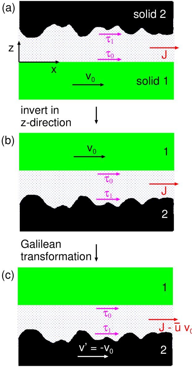
Figure 3: Mapping used to show how the flow factors change when the surface roughness of the two surfaces is interchanged.

We first invert the system along the $z$-direction. This leaves the flow current unchanged. Next we make a Galilean transformation to a new reference frame where the upper solid is stationary and the lower solid moves with the velocity $\mathbf{v}^{\prime}=-\mathbf{v}_{0}$. In the new reference frame the flow current equals $\mathbf{J}_{\mathrm{new}}=\mathbf{J}-\bar{u}\mathbf{v}_{0}$. For the original sliding system (case A; see Fig. 3(a)) the average fluid flow current is given by (5) so that for the final system (case B, Fig. 3):

$$\mathbf{J}_{\mathrm{new}}=\mathbf{J}-\bar{u}\mathbf{v}_{0}$$

$$=-{\frac{\bar{u}^{3}\phi_{\mathrm{p}}(\bar{u})}{12\eta}}\nabla\bar{p}_{\mathrm{fluid}}+{\frac{1}{2}}\bar{u}\mathbf{v}_{0}+{\frac{1}{2}}h_{\mathrm{rms}}\phi_{\mathrm{s}}(\bar{u})\mathbf{v}_{0}-\bar{u}\mathbf{v}_{0}$$

$$=-{\frac{\bar{u}^{3}\phi_{\mathrm{p}}(\bar{u})}{12\eta}}\nabla\bar{p}_{\mathrm{fluid}}-{\frac{1}{2}}\bar{u}\mathbf{v}_{0}+{\frac{1}{2}}h_{\mathrm{rms}}\phi_{\mathrm{s}}(\bar{u})\mathbf{v}_{0}$$

$$=-{\frac{\bar{u}^{3}\phi_{\mathrm{p}}(\bar{u})}{12\eta}}\nabla\bar{p}_{\mathrm{fluid}}+{\frac{1}{2}}\bar{u}\mathbf{v}^{\prime}-{\frac{1}{2}}h_{\mathrm{rms}}\phi_{\mathrm{s}}(\bar{u})\mathbf{v}^{\prime}.$$

Hence, denoting $\mathbf{v}^{\prime}$ with $\mathbf{v}_{0}$ for simplicity, we get

$$\mathbf{J}_{\mathrm{new}}=-{\frac{\bar{u}^{3}\phi_{\mathrm{p}}(\bar{u})}{12\eta}}\nabla\bar{p}_{\mathrm{fluid}}+{\frac{1}{2}}\bar{u}\mathbf{v}_{0}-{\frac{1}{2}}h_{\mathrm{rms}}\phi_{\mathrm{s}}(\bar{u})\mathbf{v}_{0}.$$

Thus the flow current for case B (the sliding system (c) in Fig. 3) can be obtained from that of case A (the original sliding system (a) in Fig. 3) by replacing $\phi_{\mathrm{s}}$ with $-\phi_{\mathrm{s}}$, while $\phi_{\mathrm{p}}$ is unchanged.

2.3 The frictional shear stress

Let us now study the frictional stress acting on the solids at the interface. We are interested in the locally averaged (effective) frictional stress $\bar{\tau}_{\mathrm{f}}=\langle\tau_{\mathrm{f}}(\mathbf{x})\rangle$. This is obtained by averaging $\tau_{\mathrm{f}}(\mathbf{x})$ over small surface areas of size $\sim\lambda\times\lambda$, where $\lambda$ is the wavelength of the longest (relevant) surface roughness component. The effective frictional stress has a contribution from the area of real contact and another from the fluid in the non-contact area, and we write

$$\bar{\tau}_{\mathrm{f}}=\bar{\tau}_{\mathrm{cont}}+\bar{\tau}_{\mathrm{fluid}}.$$

The (nominal) frictional stress resulting from the area of solid-solid contact acting on the lower surface (we assume the lower surface to be moving with the velocity $v_{0}$ while the upper solid is stationary) is derived in Appendix A:

$$\bar{\tau}_{\mathrm{cont}}^{\mathrm{up}}(x,t)=\tau_{1}{\frac{A_{1}(x,t)}{A_{0}}}-\bar{p}_{\mathrm{cont}}(x,t)\times$$

$$\left[{E_{\rm r}^{\rm up}\over E_{\rm r}^{\rm up}+E_{\rm r}^{\rm down}}\nabla\bar{u}^{\mathrm{up}}(x,t)+{E_{\rm r}^{\rm down}\over E_{\rm r}^{\rm up}+E_{\rm r}^{\rm down}}\nabla\bar{u}^{\rm down}(x,t)\right],$$

where the shear stress $\tau_{1}$ is positive when the sliding direction is along the positive $x$-direction, and negative otherwise. Note that $A_{1}(x,t)=A(x,t,\zeta_{1})$ is the area of real contact at the highest magnification, and $A_{0}$ the nominal contact area (of the elementary volume of roughness). $\bar{u}^{\mathrm{down}}(x,t)$ and $\bar{u}^{\mathrm{up}}(x,t)$ are the locally averaged (deformed) lower and upper surface, with $\bar{u}(x,t)=\bar{u}^{\mathrm{up}}(x,t)-\bar{u}^{\mathrm{down}}(x,t)$. The term proportional to $\bar{p}_{\mathrm{cont}}$ is the solid macro-rolling friction contribution acting on the upper solid, coming from the projection, onto the sliding direction, of the effective solid contact elementary forces. A similar friction stress (but with opposite sign on the adhesion contribution) acts on the upper solid:

$$\bar{\tau}_{\mathrm{cont}}^{\mathrm{down}}(x,t)=-\bar{\tau}_{\mathrm{cont}}^{\mathrm{up}}(x,t)$$

In this paper we consider only the line contact case, and in this case all mean field quantities, e.g., the local area of contact $A(x,y)$, depends only on $x$, as already assumed above. Furthermore, in the present calculations we neglect the adhesion between the solids. This is a valid assumption for positive spreading pressures, in which case there will be an effective short-ranged repulsion between the surfaces. Here we will also assume that the shear stress $\tau_{1}$ is independent of the local pressure and of the sliding speed. For most materials, e.g., rubber, $\tau_{1}$ will depend on the sliding speed but to illustrate the effect of the fluid dynamics on the friction, we prefer to keep $\tau_{1}$ as a constant.

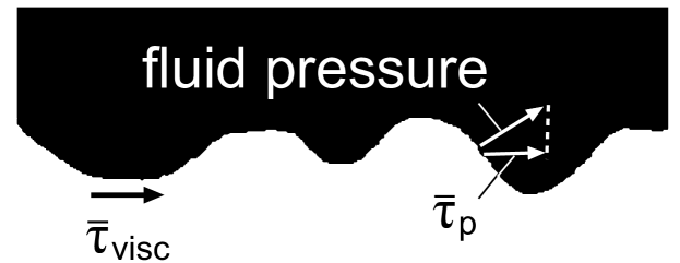
Figure 4: The shear stress acting on the solid walls from the fluid has a contribution $\tau_{\mathrm{visc}}$ from shearing the viscous fluid (proportional to the fluid viscosity) and a second contribution $\tau_{\mathrm{p}}$ from the tangential component of the fluid pressure $p(x,y)$ acting on the solid wall.

The effective frictional shear stress $\bar{\tau}_{\mathrm{fluid}}$ originating from the fluid has, in general, two contributions (see Fig. 4):

$$\bar{\tau}_{\mathrm{fluid}}=\bar{\tau}_{\mathrm{visc}}+\bar{\tau}_{\mathrm{p}}.$$

The first term $\bar{\tau}_{\mathrm{visc}}$ is determined by the effective shear stresses acting on the solid walls, whereas a second term $\bar{\tau}_{\mathrm{p}}$ is due to the projection of the effective fluid pressure forces along the sliding direction, i.e., $\bar{\tau}_{\mathrm{p}}^{\mathrm{down}}=\bar{p}_{\mathrm{fluid}}(x,t)\nabla{\bar{u}}^{\mathrm{down}}(x,t)$ for the lower surface, and ${\bar{\tau}}_{\mathrm{p}}^{\mathrm{up}}=-\bar{p}_{\mathrm{fluid}}(x,t)\nabla{\bar{u}}^{\mathrm{up}}(x,t)$ for the upper surface, where ${\bar{u}}^{\mathrm{down}}(x,t)=\left\langle u^{\mathrm{down}}(x,y,t)\right\rangle$ and ${\bar{u}}^{\mathrm{up}}(x,t)=\left\langle u^{\mathrm{up}}(x,y,t)\right\rangle$ are the locally-averaged (deformed) surface of the bottom and upper solid, respectively (as before). Thus, $\bar{\tau}_{\mathrm{visc}}$ takes into account the rough nature of the contact in the determination of the local effective frictional stresses, and in particular we show in the following that $\bar{\tau}_{\mathrm{visc}}$ includes a contribution coming from the projection of the local (asperity-scale) fluid pressure forces along the sliding direction (which we refer to as a micro-rolling friction term). The fluid shear stress is given by

$$\tau_{\mathrm{visc}}=\eta{\frac{\partial v_{x}}{\partial z}},$$

and on the bottom (down) and upper (up) surfaces it reads, respectively (all quantities depends on time but this variable is here and in what follows suppressed for convenience),

$$\tau_{\mathrm{visc}}^{\mathrm{down}}\left(\mathbf{x}\right)=-\frac{\eta\mathbf{v}_{0}}{u(\mathbf{x})}-{\frac{1}{2}}u(\mathbf{x})\nabla p(\mathbf{x}),$$

$$\tau_{\mathrm{visc}}^{\mathrm{up}}\left(\mathbf{x}\right)=\frac{\eta\mathbf{v}_{0}}{u(\mathbf{x})}-{\frac{1}{2}}u(\mathbf{x})\nabla p(\mathbf{x}),$$

resulting in

$$\tau_{\mathrm{fluid}}^{\mathrm{down}}\left(\mathbf{x}\right)=\tau_{\mathrm{visc}}^{\mathrm{down}}\left(\mathbf{x}\right)+p(\mathbf{x})\nabla u^{\mathrm{down}}(\mathbf{x}),$$

$$\tau_{\mathrm{fluid}}^{\mathrm{up}}\left(\mathbf{x}\right)=\tau_{\mathrm{visc}}^{\mathrm{up}}\left(\mathbf{x}\right)-p\left(\mathbf{x}\right)\nabla u^{\mathrm{up}}(\mathbf{x}).$$

Here $p=p_{\mathrm{fluid}}$ for simplicity of notation.

We will now calculate $\bar{\tau}_{\mathrm{fluid}}$ for one case only, namely when the upper solid is elastic and has random surface roughness and the lower solid is rigid and with a flat surface (no surface roughness). The other cases of interest can be studied in a similar way, and the derivation and results are given in Appendix B.

For the bottom surface: Since the bottom surface is flat and rigid, $\nabla u^{\mathrm{down}}=0$ and hence $\tau_{\mathrm{fluid}}^{\mathrm{down}}=\tau_{\mathrm{visc}}^{\mathrm{down}}$. Using (12a) we get in this case (see also Ref. MS2 ):

$$\langle\tau_{\mathrm{visc}}\rangle=\bar{\tau}_{\mathrm{visc}}=-\phi_{\mathrm{f}}\frac{\eta_{0}\mathbf{v}_{0}}{\bar{u}}-{\frac{1}{2}}\left\langle u\nabla p\right\rangle,$$

whereMS2

$$\phi_{\mathrm{f}}=\left\langle{\frac{\eta}{u(\mathbf{x})}}\right\rangle{\frac{\bar{u}}{\eta_{0}}},$$

where $\eta_{0}$ is the low shear rate fluid viscosity. Furthermore, for $\bar{u}<\bar{u}_{\mathrm{c}}$ (where $\bar{u}_{\mathrm{c}}$ is the average interfacial separation at the point when the contact area percolate)

$$\langle u\nabla p\rangle=6\eta_{0}\mathbf{v}_{0}\bar{u}\left\langle{\frac{1}{u}}\right\rangle.$$

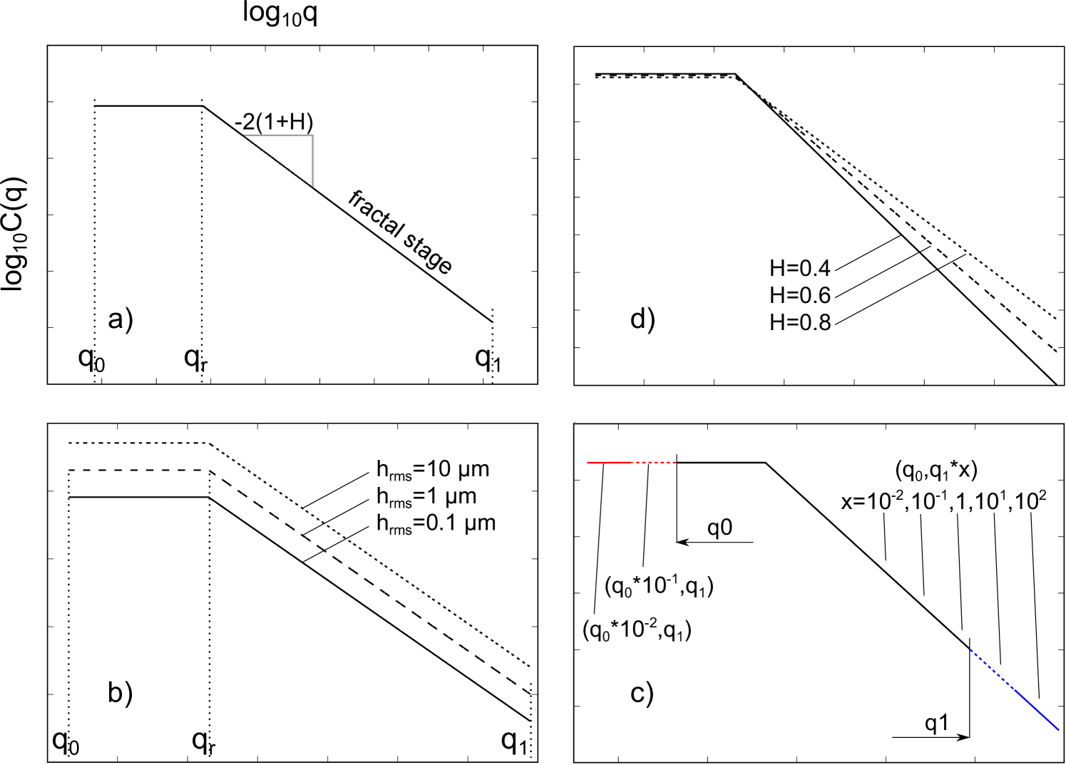
Figure 5: Schematic of the power spectral density (PSD) adopted to elucidate the role of roughness properties on the flow and friction factors. (a) The reference surface is characterized by a fractal content in the range of frequencies $\left[q_{\mathrm{r}},q_{1}\right]$, and a flat (roll-off) PSD in $\left[q_{0},q_{\mathrm{r}}\right]$. The latter PSD range provides a simplified mathematical representation of the typical decaying PSD behavior, at increasing wavenumbers, shown by real surfaces. (b) The comparison is made at constant wavenumbers and fractal dimension, but at varying rms surface roughness $h_{\mathrm{rms}}$. (c) Here $h_{\mathrm{rms}}$ and the fractal dimension are kept constant, whereas the wavenumbers $q_{0}$ and $q_{1}$ are alternately varied. Finally, (d) both wavenumbers $q_{0}$ and $q_{1}$, and $h_{\mathrm{rms}}$ are kept fixed, but the Hurst exponent $H$ ($H=3-D_{\mathrm{f}}$, where $D_{\mathrm{f}}$ is the fractal dimension) is varied.

On the other hand for $\bar{u}>>h_{\mathrm{rms}}$ one has MS2

$$\langle u\nabla p\rangle=\left(1-3D{\frac{\langle h^{2}\rangle}{\bar{u}^{2}}}\right)\bar{u}\nabla\bar{p}+6D{\frac{\langle h^{2}\rangle}{\bar{u}^{2}}\frac{\eta_{0}\mathbf{v}_{0}}{\bar{u}},}$$

where $\bar{p}=p_{\mathrm{fluid}}$. The general form for (16) and (17) is

$$\langle u\nabla p\rangle=\phi_{\mathrm{fp}}\bar{u}\nabla\bar{p}+\phi_{\mathrm{fs}}\frac{2\mathbf{v}_{0}\eta_{0}}{\bar{u}},$$

where the relations for $\phi_{\mathrm{fp}}$ and $\phi_{\mathrm{fs}}$, obtained by interpolation, are given in Ref. MS2 :

$$\phi_{\mathrm{fs}}={\frac{3\bar{u}}{\langle u^{-1}\rangle^{-1}+\theta(\bar{u}-\bar{u}_{\mathrm{c}})(\bar{u}-\bar{u}_{\mathrm{c}})(\bar{u}^{2}/\langle h^{2}\rangle)D^{-1}}},$$

and

$$\phi_{\mathrm{fp}}={\frac{\bar{u}(\bar{u}-\bar{u}_{\mathrm{c}})\theta(\bar{u}-\bar{u}_{\mathrm{c}})}{\bar{u}^{2}+3\langle h^{2}\rangle D}},$$

where $\theta(u)$ is the unit step function and the surface roughness anisotropic parameter, $D$, is related to the Tripp number $\gamma$ with $D=\left(1+\gamma\right)^{-1}$ MS2 . Substituting (18) in (14) gives the effective frictional shear stress acting on the bottom solid

$$\bar{\tau}_{\mathrm{visc}}^{\mathrm{down}}=-\left(\phi_{\mathrm{f}}+\phi_{\mathrm{fs}}\right){\frac{\eta_{0}\mathbf{v}_{0}}{\bar{u}}}-\frac{1}{2}\phi_{\mathrm{fp}}\bar{u}\nabla\bar{p}.$$

where $\phi_{\mathrm{f}}$, $\phi_{\mathrm{fs}}$ and $\phi_{\mathrm{fp}}$ are given by (15), (19) and (20).

For the top surface: The top surface has surface roughness and the fluid rolling term

$$p({\bf x})\nabla u({\bf x}),$$

is non-vanishing, where $u^{\mathrm{up}}({\bf x})=u({\bf x})$ in this case. Hence on the top surface the fluid acts with the local friction shear stress

$$\tau_{\mathrm{fluid}}^{\mathrm{up}}=\tau_{\mathrm{visc}}^{\mathrm{up}}-p\left(\mathbf{x}\right)\nabla u\left(\mathbf{x}\right).$$

From (13) and (23) we get

$$\langle\tau_{\mathrm{fluid}}^{\mathrm{up}}\rangle=\bar{\tau}_{\mathrm{fluid}}^{\mathrm{up}}=\left\langle{\frac{\eta\mathbf{v}_{0}}{u}}\right\rangle-{\frac{1}{2}}\langle u\nabla p\rangle-\langle p\nabla u\rangle.$$

To second order in the rms-roughness amplitude one has (see Ref. MS2 ):

$$\left\langle p\nabla u\right\rangle=\left\langle p_{1}\nabla u_{1}\right\rangle+\bar{p}\nabla\bar{u},$$

and

$$\left\langle u\nabla p\right\rangle=\left\langle u_{1}\nabla p_{1}\right\rangle+\bar{u}\nabla\bar{p}.$$

Next, using Eqs. (A5)-(A9) in Ref. MS2 it is easily shown that

$$\left\langle p_{1}\nabla u_{1}\right\rangle=-\left\langle u_{1}\nabla p_{1}\right\rangle.$$

Using (25)-(27) we get

$$\left\langle p\nabla u\right\rangle=-\left\langle u\nabla p\right\rangle+\bar{p}\nabla\bar{u}+\bar{u}\nabla\bar{p}.$$

Substituting (28) in (24) gives

$$\bar{\tau}_{\mathrm{fluid}}^{\mathrm{up}}=\left\langle\frac{\eta}{u}\right\rangle\mathbf{v}_{0}+{\frac{1}{2}}\left\langle u\nabla p\right\rangle-\bar{u}\nabla\bar{p}-\bar{p}\nabla\bar{u},$$

The last term in (29), $-\bar{p}\nabla\bar{u}$, is the fluid macro-rolling frictional shear stress $\bar{\tau}_{\mathrm{p}}^{\mathrm{up}}$ (since $-\bar{p}\nabla\bar{u}^{\mathrm{up}}=-\bar{p}\nabla\bar{u}$, given the bottom rigid and flat surface). Using (15), (18) and (29) we get

$$\bar{\tau}_{\mathrm{fluid}}^{\mathrm{up}}=\left(\phi_{\mathrm{f}}+\phi_{\mathrm{fs}}\right){\frac{\eta_{0}\mathbf{v}_{0}}{\bar{u}}}+{\frac{1}{2}}(\phi_{\mathrm{fp}}-2)\bar{u}\nabla\bar{p}-\bar{p}\nabla\bar{u}.$$

We do note that the global mechanical equilibrium along the sliding direction is conserved, i.e.

$$\int_{x_{a}}^{x_{b}}dx\leavevmode\nobreak\ \bar{\tau}_{\mathrm{fluid}}^{\mathrm{down}}+\int_{x_{a}}^{x_{b}}dx\leavevmode\nobreak\ \bar{\tau}_{\mathrm{fluid}}^{\mathrm{up}}+\bar{p}_{\mathrm{out}}\bar{u}_{\mathrm{out}}-\bar{p}_{\mathrm{in}}\bar{u}_{\mathrm{in}}=0,$$

where $\bar{p}_{\mathrm{out}}$ ($\bar{p}_{\mathrm{in}}$) and $\bar{u}_{\mathrm{out}}$ ($\bar{u}_{\mathrm{in}}$) are, respectively, the average fluid pressure and separation at the contact outlet (inlet).

2.4 Dependence of flow and friction factors on roughness parameters

In this section we present numerical results for the fluid flow factors $\phi_{\mathrm{p}}$ and $\phi_{\mathrm{s}}$, and for the frictional stress factors $\phi_{\mathrm{f}}$, $\phi_{\mathrm{fs}}$ and $\phi_{\mathrm{fp}}$, for solids with different surface roughness. Note that the accurate description of the flow and shear stress factors, and of the asperity-asperity contact, is crucial in the formulation of any mean field lubrication theory.

The power spectral densities (PSD) $C(q)$ adopted in this section are shown in Fig. 5. Fig. 5(a) shows the PSD of a surface with a (self affine) fractal region between the roll-off wavenumber $q_{\mathrm{r}}$ and the large wavenumber cut-off $q_{1}$. Most surfaces of engineering interest have a nearly flat roll-off region $q_{0}<q<q_{\mathrm{r}}$, where $C(q)$ is almost constantPersson2005 . Fig. 5(b) shows three power spectra with the same $q_{0}$, $q_{\mathrm{r}}$ and $q_{1}$ wavenumbers, and the same fractal dimension, but with different rms surface roughness $h_{\mathrm{rms}}$. Fig. 5(c) shows the case where $h_{\mathrm{rms}}$ and the fractal dimension are kept constant, whereas the large and small wavenumber cut-off are varied. Finally, in Fig. 5(d) both the cut-off and roll-off wavenumbers and $h_{\mathrm{rms}}$ are fixed, but the Hurst exponent $H$ ($H=3-D_{\mathrm{f}}$, where $D_{\mathrm{f}}$ is the fractal dimension) is varied.

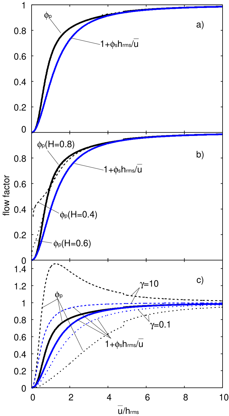
Figure 6: The mean field correction to the Poiseuille flow $\phi_{\mathrm{p}}$ (black lines) and the mean field correction to the Couette flow $\left(1+\phi_{\mathrm{s}}h_{\mathrm{rms}}/\bar{u}\right)$ (blue lines), as a function of the dimensionless average interface separation $\bar{u}/h_{\mathrm{rms}}$. In particular, in (a) we vary $h_{\mathrm{rms}}$, the small wavenumber cut-off $q_{0}$ and the large wavenumber cut-off $q_{1}$, whereas in (b) we vary the Hurst exponent $H$ and in (c) we vary the Tripp number.

The reference PSD has the small wavenumber cut-off $q_{0}=2\times 10^{3}\leavevmode\nobreak\ \mathrm{m}^{-1}$, the roll-off wavenumber $q_{r}=2\times 10^{5}\leavevmode\nobreak\ \mathrm{m}^{-1}$, the large wavenumber cut-off $q_{1}=7.8\times 10^{9}\leavevmode\nobreak\ \mathrm{m}^{-1}$, the rms roughness $h_{\mathrm{rms}}=1\leavevmode\nobreak\ \mathrm{\mu m}$ and the Hurst exponent $H=0.8$. The reference PSD correspond to a surface with the rms-slope $2.45$, so the surface with the rms-roughness $10\ \mathrm{\mu m}$, and the surfaces with the Hurst exponent $H=0.6$ and $0.4$ will have too large rms-slope to be physically reasonable, but for the present parameter study this is not very important. In what follows we assume that the elastic solid has the reduced Young’s modulus $E_{\mathrm{r}}=6.67\leavevmode\nobreak\ \mathrm{MPa}$, and the fluid is assumed to be Newtonian.

In Fig. 6 we show the mean field correction to the Poiseuille flow $\phi_{\mathrm{p}}$ (black lines) and the mean field correction to the Couette flow $\left(1+\phi_{\mathrm{s}}h_{\mathrm{rms}}/\bar{u}\right)$ (blue lines), as a function of the dimensionless average interface separation $\bar{u}/h_{\mathrm{rms}}$. In Fig. 6(a) we vary $h_{\mathrm{rms}}$, the small wavenumber cut-off $q_{0}$ and the large wavenumber cut-off $q_{1}$, whereas in (b) we vary the Hurst exponent $H$ and in (c) we vary the Tripp number. In Fig. 6(a) all curves superpose, i.e., the flow factors as a function of $\bar{u}/h_{\mathrm{rms}}$ are not sensitive to $q_{0}$, $q_{1}$ and $h_{\mathrm{rms}}$, at least not in the parameter range studied here. This is, however, not the case when we vary the Hurst exponent $H$ (see Fig. 6(b)) or the Tripp number $\gamma$ (see Fig. 6(c)). Let us explain for the pressure flow factor $\phi_{\mathrm{p}}$ the physical origin of this.

When we decrease the Hurst exponent, the roughness at short length scales increases, while the long wavelength roughness is nearly unchanged (assuming a fixed $h_{\mathrm{rms}}$ roughness amplitude). This implies that when $H$ decreases the surface rms-slope increases, which in turn decreases the contact area. Thus the pressure needed for the contact area to percolate (at which point $\phi_{\mathrm{p}}$ vanish) will increase when $H$ decreases. Since increasing pressure implies decreasing average interfacial separation it follows that the value of $\bar{u}/h_{\mathrm{rms}}$ where $\phi_{\mathrm{p}}$ first vanish will decrease as $H$ decreases, in agreement with Fig. 6(b). Here we have used that the average interfacial separation is mainly determined by the long wavelength roughness and therefore only weakly dependent on the Hurst exponent, assuming a constant $h_{\mathrm{rms}}$.

Fig. 6(c) shows that when we increase the Tripp number the fluid pressure flow factor increases. Since the pressure flow factor defines an effective viscosity $\eta_{\mathrm{eff}}=\eta/\phi_{\mathrm{p}}$ (see Sec. 2.1), this is equivalent to the statement that an increasing Tripp number result in a lower effective viscosity. This is easy to understand since a large Tripp number $\gamma>>1$ implies that there are roughness channels (in our case grinding scratches) along the fluid flow direction (i.e., orthogonal to the cylinder axis), which facilitate the flow of the fluid out from the nominal contact area. In the opposite limit $\gamma<<1$ the flow channels are orthogonal to the fluid flow direction (i.e. along the cylinder axis) which inhibit fluid squeeze-out and result in an effective viscosity which is larger than the bare viscosity for all interfacial separations.

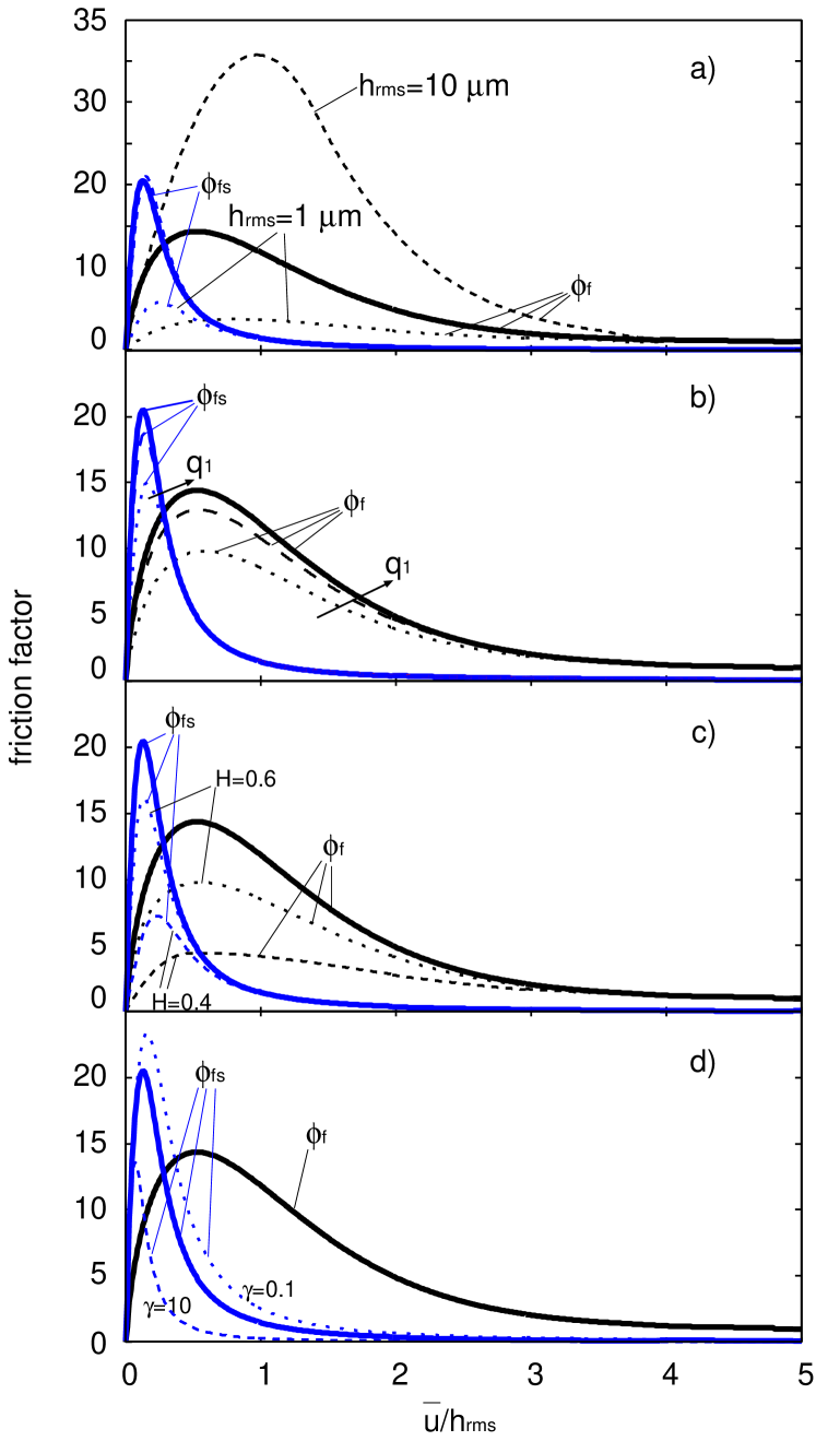
Figure 7: The mean field correction to the sliding shear stress ($\eta v_{0}/\bar{u}$) $\phi_{\mathrm{f}}$ (black lines) and $\phi_{\mathrm{fs}}$ (blue lines), as a function of the dimensionless average interface separation $\bar{u}/h_{\mathrm{rms}}$. In (a) we vary $h_{\mathrm{rms}}$ and the small wavenumber cut-off $q_{0}$, in (b) the large wavenumber cut-off $q_{1}$, in (c) the dependence on the fractal dimension and in (d) on the Tripp number.

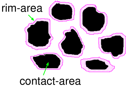
Figure 8: The contact area (black) and the rim area (pink). The most important contribution to $\langle u^{-1}\rangle$ comes from the pink area, i.e., from relative narrow strips of surface area at the rim of the contact area, where the surface separation is very small.

Figure 9: The mean field correction to the pressure gradient friction term ($\bar{u}\nabla p$) $\phi_{\mathrm{fp}}$ as a function of the dimensionless average interface separation $\bar{u}/h_{\mathrm{rms}}$. In particular, in (a) we vary $h_{\mathrm{rms}}$, the small wavenumber cut-off $q_{0}$ and the large wavenumber cut-off $q_{1}$ as well as the Hurst exponent $H$, whereas in (b) we vary the Tripp number.

In Fig. 7 we show the mean field correction $\phi_{\mathrm{f}}$ (black lines) to the sliding shear stress ($\eta v_{0}/\bar{u}$), and $\phi_{\mathrm{fs}}$ (blue lines), as a function of the dimensionless average interface separation $\bar{u}/h_{\mathrm{rms}}$. In Fig. 7(a) we show the dependence on $h_{\mathrm{rms}}$ and on the small wavenumber cut-off $q_{0}$. In Fig. 7(b) we vary the large wavenumber cut-off $q_{1}$, in Fig. 7(c) the fractal dimension, and in Fig. 7(d) the Tripp number. We first remark that $q_{0}$ has a negligible influence on the sliding shear stress (curves are superposed), whereas $q_{1}$, $h_{\mathrm{rms}}$ and $D_{\mathrm{f}}$ do influence the sliding shear stresses.

Fig. 7(a) shows that $\phi_{\mathrm{f}}$ increases with increasing $h_{\mathrm{rms}}$. This can be understood from the definition $\phi_{\mathrm{f}}\sim\left\langle\bar{u}/u\right\rangle=\bar{u}\langle u^{-1}\rangle$. Now, as $h_{\mathrm{rms}}$ becomes larger $\bar{u}$ will increase too [at low nominal contact pressures it is nearly proportional to $h_{\mathrm{rms}}$ (see Persson2007 )]. The quantity $\langle u^{-1}\rangle$ has its biggest contribution from the surface area where the separation $u$ is very small. This surface area is located in a narrow rim around the area of real contact (see Fig. 8). We will denote the non-contact surface area, where the surface separation is below, say $u<10\ \mathrm{nm}$, as the rim area. If $h_{\mathrm{rms}}$ is increased by adding only long-wavelength roughness to the surface profile then the rms-slope, and hence also the area of real contact, and the rim area, are nearly unchanged. In this case $\langle u^{-1}\rangle$ will be nearly unchanged, and $\phi_{\mathrm{f}}$ will increase with increasing $h_{\mathrm{rms}}$. However, in the present case the surface roughness height is scaled everywhere by a multiplicative factor, say $\zeta$ [equal to 10 or 0.1 in Fig. 7(a)]. In this case, at a constant applied pressure, if $\zeta$ increases, $\bar{u}$ will increase with roughly a factor of $\zeta$, while the contact area will decrease with roughly a factor $1/\zeta$. However, it is likely that the rim area will decrease slower with $\zeta$ then the surface area since it depends on the length of the boundary lines of the contact area which may decrease slower than the area itself. This would explain why $\phi_{\mathrm{f}}$, as a function of $\bar{u}/h_{\rm rms}$, increases as $h_{\mathrm{rms}}$ increases.

Similar considerations apply to $\phi_{\mathrm{fs}}$ in the range of average interface separation $\bar{u}<u_{\mathrm{c}}$, where again $\phi_{\mathrm{fs}}\sim\left\langle\bar{u}/u\right\rangle$. At larger separations, instead, all $\phi_{\mathrm{fs}}$ curves in Fig. 7(a) converge to a unique mastercurve, being $\phi_{\mathrm{fs}}\sim{h_{\mathrm{rms}}^{2}/}\bar{u}^{2}$.

Fig. 7(b) shows that when the large wavenumber cut-off $q_{1}$ increases, $\phi_{\rm f}$ increases too. This can be understood as follows: Note that $\bar{u}$ is mainly determined by the long wavelength roughness and hence does not depend on the cut-off $q_{1}$ unless $\bar{u}/h_{\rm rms}<<1$. We now consider the change in the contact as we move from the cut-off $q_{1}^{\prime}=0.1q_{1}$ to $q_{1}$. We consider first the system with the largest wavenumber cut-off and write $q=\zeta q_{0}$ with $q_{1}=\zeta_{1}q_{0}$. When we increase the magnification $\zeta$ the contact area decreases, i.e., new non-contact area appears in what appeared to be contact at a lower magnification. When the magnification is increased to $\zeta=0.1\zeta_{1}$ we observe what is essentially the contact as it would prevail for the system with the cut-off $q^{\prime}_{1}=0.1q_{1}$. When we increase the magnification from $\zeta=0.1\zeta_{1}$ to $\zeta=\zeta_{1}$ some regions which appeared to be in contact at the magnification $\zeta=0.1\zeta_{1}$, will now be observed to be non-contact regions with closely spaced surfaces, while the non-contact regions observed at the magnification $\zeta=0.1\zeta_{1}$ will still be non-contact regions with nearly the same surface separation as observed at the lower magnification. The “additional” non-contact area (with closely spaced surfaces) observed when increasing the magnification from $\zeta=0.1\zeta_{1}$ to $\zeta=\zeta_{1}$ will result in an important additional contribution to $\langle u^{-1}\rangle$. We conclude that $\phi_{\rm f}$ as a function of $\bar{u}/h_{\rm rms}$ will increase as $q_{1}$ increases.

When the fractal dimension increases (or Hurst exponent $H$ decreases), both $\phi_{\mathrm{f}}$ and $\phi_{\mathrm{fs}}$ decreases as shown in Fig. 7(c). This is easy to understand. When $H$ decreases the amplitude of the short wavelength roughness increases, while the long wavelength roughness, assuming a constant $h_{\mathrm{rms}}$, change very little. When the short wavelength roughness increases, the surface rms-slope and hence the surface area decreases. This imply that the rim area and hence also $\langle u^{-1}\rangle$ decreases as the Hurst exponent $H$ decreases. It follows that $\phi_{\mathrm{f}}$ will decrease when the fractal dimension increases at constant $h_{\mathrm{rms}}$.

Fig. 7(d) shows that $\phi_{\mathrm{f}}$ is unaffected by the anisotropy (Tripp number $\gamma$) of the surface. This is indeed expected because both the contact area (and the rim area) and the average surface separation are nearly independent of the surface anisotropy assuming identical angular averaged surface roughness power spectrum. Indeed, this hold exactly within the Persson’s contact mechanics theory where only the angular-averaged power spectral density Carbone2009 enters. As a consequence, $\phi_{\mathrm{f}}$ is unaffected by the Tripp number. The situation is different in the case of $\phi_{\mathrm{fs}}$, which at larger separation $\phi_{\mathrm{fs}}\sim D$, where $D=\left(1+\gamma\right)^{-1}$.

Finally, in Fig. 9 we show $\phi_{\mathrm{fp}}$, which is the mean field correction to the pressure gradient friction term, $\bar{u}\nabla p$, as a function of the dimensionless average interface separation $\bar{u}/h_{\mathrm{rms}}$. In Fig. 9(a) we vary $h_{\mathrm{rms}}$, the small wavenumber cut-off $q_{0}$ and the large wavenumber cut-off $q_{1}$ as well as the Hurst exponent $H$, whereas in Fig. 9(b) we vary the Tripp number. Here $\phi_{\mathrm{fp}}$ is mainly sensitive to the Tripp number through its dependence with $D$. However, differently from $\phi_{\mathrm{fs}}$, $\phi_{\mathrm{fp}}$ increases at increasing Tripp numbers. Thus, given the opposite behaviors shown by the various frictional sources ($\phi_{\mathrm{f}}$, $\phi_{\mathrm{fs}}$ and $\phi_{\mathrm{fp}}$) originating from the fluid viscous dissipation in anisotropically rough contacts, it is not possible to establish a general statement about the role of the Tripp number in wet contact mechanics, since the total friction will be determined by the relative weight and the variation of such friction factors terms along the effective contact domain. However, qualitatively, a mixed lubrication occurring under $\eta v_{0}/\left|\nabla p\right|\gg\bar{u}^{2}$, thus at relatively large values of contact pressures (leading to a small average interface separation) will be characterized by larger friction for transverse roughness than for longitudinal roughness, in agreement with experimental findings MS7 . For $\bar{u}^{2}\gg\eta v_{0}/\left|\nabla p\right|$, instead, the contact is expected to occur under small true contact area, leading to large interfacial separation and thus to larger friction for the longitudinal roughness than for the transverse roughness. The latter case will be discussed in the comparison with experimental results provided in the following.

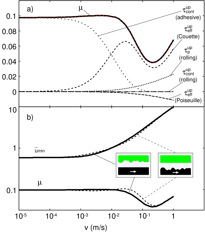
Figure 10: (a) The friction (black solid line) and the corresponding dissipation terms (other black lines) originating on the cylinder, as a function of the sliding speed. The solid black line is for the case of a rough steady cylinder of radius $R=2.5\leavevmode\nobreak\ \mathrm{mm}$ squeezed against a flat ideally smooth rigid sliding counter surface, under constant normal line load $F_{\mathrm{N}}=100\leavevmode\nobreak\ \mathrm{N/m}$. we consider a solid with a reduced elastic modulus $E_{\mathrm{r}}=6.67\leavevmode\nobreak\ \mathrm{MPa}$, as well as a Newtonian fluid, with dynamic viscosity $\eta=0.1\leavevmode\nobreak\ \mathrm{Pas}$. The shear stress occurring in the true contact areas is assumed constant and valued $\sigma_{\mathrm{f}}=1\leavevmode\nobreak\ \mathrm{MPa}$. The sliding speed is in the range between $10^{-5}$ and $1\leavevmode\nobreak\ \mathrm{m/s}$. The red solid line, instead, is for the same contact conditions of before but with the elasticity assigned to the bottom sliding surface (i.e. the cylinder is rigid and the substrate is deformable). (b) The friction coefficient (the lower solid and dashed lines) and the minimum average separation (the upper solid and dashed lines), as a function of the sliding speed, for the same contact condition of (a), but for the case of roughness on the cylinder (solid lines) or on the substrate (dashed lines). The full and dashed lines are for the cases where the cylinder is rigid and compliant, respectively.

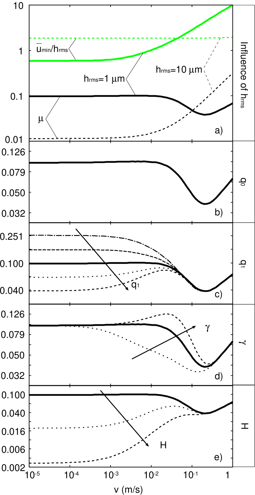
Figure 11: The friction as a function of the sliding speed, for the same parameters of Fig. 10(a) but for (from top to bottom): (a) varying $h_{\mathrm{rms}}$, (b) $q_{0}$, (c) $q_{1}$, (d) $\gamma$ and (e) Hurst exponent. The PSDs are described in Fig. 5.

2.5 Dependence of lubricated friction on roughness parameters

In this section we present numerical results for the Stribeck curve, for solids with different surface roughness. The power spectral densities (PSD) $C(q)$ adopted in this section are shown in Fig. 5. Again we consider a solid with reduced elastic modulus $E_{\mathrm{r}}=6.67\leavevmode\nobreak\ \mathrm{MPa}$, and assume a Newtonian fluid with the dynamic viscosity $\eta=0.1\leavevmode\nobreak\ \mathrm{Pas}$. The flow and friction factors used in the calculation below are those discussed before. In the following, unless differently specified, we consider a stationary cylinder of radius $R=2.5\leavevmode\nobreak\ \mathrm{mm}$, and with random surface roughness, squeezed against a flat ideally smooth sliding (speed $v_{0}$) counter surface. On the cylinder we apply the normal (line contact) load per unit length $F_{\mathrm{N}}/L=100\leavevmode\nobreak\ \mathrm{N/m}$, and the shear stress occurring in the true contact areas is assumed constant $\tau_{1}=1\leavevmode\nobreak\ \mathrm{MPa}$. The sliding speed is varied from $10^{-5}$ to $1\leavevmode\nobreak\ \mathrm{m/s}$.

We write the friction force acting on the cylinder as $F=\mu F_{\mathrm{N}}$. In Fig. 10(a) we show the friction coefficient $\mu$ (solid line), and the different contributions to the friction coefficient (dashed lines), as a function of the sliding speed. Thus, from top to bottom:

(1) the adhesive contribution to friction (i.e. the friction coming from the shearing action occurring in true solid contact area), proportional to the shear stress $\tau^{\mathrm{up}}_{\mathrm{cont}}(\mathrm{adhesive})$,

(2) the Couette-flow term [proportional to $\tau^{\mathrm{up}}_{\mathrm{eff}}(\mathrm{Couette})$],

(3) the rolling friction originating from the fluid pressure field [proportional to $\tau^{\mathrm{up}}_{\mathrm{p}}(\mathrm{rolling})$],

(4) the rolling friction originating from the solid contact pressure field [proportional to $\tau^{\mathrm{up}}_{\mathrm{cont}}(\mathrm{rolling})$],

(5) the Poiseuille-flow term [proportional to $\tau^{\mathrm{up}}_{\mathrm{eff}}(\mathrm{Poiseuille})$].

We note that the rolling friction coming from the solid contact pressure is zero, since the substrate is nominally flat and rigid (and,anyway, no solid bulk viscoelasticy is considered in this paper). In the same figure, the red solid line (approximately superposed with the black dashed line) is for the same contact conditions of before, but with the elasticity assigned to the bottom sliding surface (i.e. the cylinder is rigid and the substrate is deformable). We note that for the adopted set of contact parameters, the friction force is the same in the two cases.

Let us now instead consider the case where the roughness is transferred from the steady cylinder to the sliding substrate. Thus in Fig. 10(b) we show the friction coefficient (the lower solid and dashed lines) and the minimum average separation (the upper solid and dashed lines), as a function of the sliding speed, for the same contact condition of Fig. 10(a), but for the case of roughness on the cylinder (solid lines) or on the substrate (dashed lines). We note, as expected, that the different allocation of the roughness does play a role only in the mixed lubrication regime, where the asperity-fluid interactions dominate the contact mechanics.

In Fig. 11 we show the friction as a function of the sliding speed (and in Fig. 11(a) also the minimum surface separation), for the same parameters as in Fig. 10(a), except that we vary (from top to bottom): (a) $h_{\mathrm{rms}}$, (b) $q_{0}$, (c) $q_{1}$, (d) $\gamma$ and (e) the Hurst exponent. Fig. 11(a) shows that when the rms roughness increases from $1\ \mathrm{\mu m}$ (solid green line) to $10\ \mathrm{\mu m}$ (dashed green line), the build up of hydrodynamic fluid pressure with increasing sliding speed is not enough to increase the average surface separation, i.e., the (nominal) fluid pressure is negligible compared to the (nominal) asperity contact pressure. Thus, for $h_{\mathrm{rms}}=10\ \mathrm{\mu m}$ the minimum interface separation does not increase with increasing sliding speed, i.e. for all velocities studied it takes the same value as in the boundary lubrication regime. Nevertheless, Fig. 11(a) shows that there is a hydrodynamic contribution to the friction force (black dashed line). This is due to the shearing of the fluid in the small asperity gaps, and is described by the $\phi_{\mathrm{f}}$ term in the expression for the frictional shear stress. Therefore, in this case the hydrodynamic contribution to the friction is a truly micro-EHL effect, i.e. a hydrodynamic effect occurring at the scale of the roughness asperities.

In Fig. 11(b) and (c), we show the effect of the large and small roughness wavelength, respectively. As expected, $q_{0}$ has negligible effect on the friction curve, because it has only very small effect on the roughness solid contact mechanics. The large frequency cut-off $q_{1}$ (and the Hurst exponent, see Fig. 11(e)), instead, has a direct influence on the solid contact mechanics, in particular through the mean square roughness slope $\langle(\nabla h)^{2}\rangle$, which increases when $q_{1}$ increases. Thus, since the true contact area $A_{\mathrm{c}}$ (in the linear regime) scales as $A_{\mathrm{c}}\propto F_{\mathrm{N}}\langle(\nabla h)^{2}\rangle^{-1/2}$, the friction coefficient in the boundary regime will be proportional to $\langle(\nabla h)^{2}\rangle^{-1/2}$. Hence, the contact area and the friction coefficient will decrease at increasing $q_{1}$ (and decreasing $H$, see Fig. 11(e)). Finally, in Fig. 11(d) we show the effect of roughness anisotropy on the friction. As anticipated, for very low sliding speed, when hydrodynamic effects are negligible, the contact area, and hence also the friction force, does not depend on the anisotropy parameter $\gamma$ (note: this is true only if there is no viscoelastic contribution to the friction; see Fig. 1 and the discussion related to this figure). However, at higher sliding speeds (when $\bar{u}^{2}\gg\eta v_{0}/\left|\nabla p\right|$), where hydrodynamic effects becomes important, when the long axis of the (on the average elliptic) asperities are aligned along the sliding direction, fluid is more easily removed from the nominal contact region, resulting in smaller surface separation and larger friction force, than when the asperities are aligned perpendicular to the sliding direction.

2.6 Some comments on mean-field lubrication models

As pointed out above, an accurate treatment of the fluid flow and friction shear stress factors, as well as of the asperity-asperity contact, is crucial in the formulation of a mean field lubrication theory. To this point we observe that, (at least) the roughness contact mechanics has been the subject of dedicated and very detailed research efforts in recent years, leading to some controversial research papers but also to some incontestable results. Among the latter outcomes we remark the recognition, by analyticalgeneral_multiscale , numericalScaraggi.in.prep ; scaraggi2016effect and experimental approacheslorenz2010leak ; lorenz2013adhesion ; lorenz2013static , of the exponential relation between the average contact pressure $p_{\mathrm{cont}}$ and interface separation $\bar{u}$ in elastic contacts for large enough surface separation [see e.g. (3)]Persson2007 , as well as of the linearity between true contact area and contact pressure (for $A(p)/A_{0}<0.3$) in both elastic and viscoelastic contactsPersson2014 , the occurrence of solid percolation and its effects on the hydraulic resistivity (see e.g. (16) and related discussion)lorenz2010leak , and many others.

As an example, consider the contact pressure vs average separation relation, $\bar{p}=p(\bar{u})$, as given by (3). This relation follows from the Persson multiscale contact mechanics approachPersson2007 in the limit of $\bar{u}/h_{\mathrm{rms}}>>1$, and is in agreement with both experimental0953-8984-21-1-015003 and numerical studiesAlmqvist20112355 , except at very low nominal contact pressures where finite size effects occursAlmqvist20112355 . Therefore, for elastic solids with randomly rough surfaces any other pressure vs separation law (and related contact mechanics theory) not showing such an exponential behavior (e.g., the GW many-noninteracting-asperity theoryGreenwood300 ), should be avoided as building block for a mean-field lubrication theory.

In a recent paper Masjedi and Khonsari Khonsari observe that similar results are obtained when adopting the GW contact mechanics, as obtained in the 2009 paper by Persson and ScaraggiMS1 , where a mean field lubrication theory was developed based on the Persson contact mechanics theory. Here we note that in Ref. Khonsari two of the three roughness parameters, namely the mean asperity radius $\beta$ and the asperity surface density $n$, where used as fitting parameters. Indeed, the authors claim that such parameters are difficult to obtain from a power spectral density Khonsari , but in fact can be calculated as described by Nayak nayak . In particular:

$$\frac{1}{\beta^{2}}=\frac{8m_{4}}{3\pi}$$

and

$$n=\frac{1}{6\pi\sqrt{3}}\frac{m_{4}}{m_{2}},$$

where

$$m_{n}=\int d^{2}q\leavevmode\nobreak\ q^{n}C\left(\mathbf{q}\right).$$

Using these equations we calculate $\beta\approx 2\leavevmode\nobreak\ \mathrm{nm}$ and $\beta nh_{\mathrm{rms}}\approx 625$, whereas the value adopted by Masjedi and Khonsari Khonsari are $\beta=0.02\ \mathrm{mm}$ and $n\beta\sigma=0.05$. Thus, the model parameters adopted in Ref. Khonsari are orders away from those really describing the true contact system; as a result, the comparison reported in Khonsari have to be reconsidered, so that further clarifying research is needed on this aspect. In addition we note that a certain discrepancy can be observed also under elasto-hydrodynamics conditions, when no asperity-asperity or asperity-fluid interactions are relevant, reported on in Fig. 1a of Ref. Khonsari . This is likely due to a different numerical inlet distance adopted by Masjedi and Khonsari, which might sensibly affect the numerical results, as confirmed by the authors. Thus, it would have been more helpful to provide numerical results for exactly the same contact conditions.

3 Experimental setup

In order to experimentally investigate the lubricated line contact of a generic hydraulic seal, a test rig has been designed and set up at the Institute for Fluid Power Drives and Controls (IFAS). Here we summarize the experimental setup, whose detailed description can be found in another contribution conf.23 . A steel cylinder (radius $R=10\ \mathrm{cm}$) is rotated through a two-stepped gearbox (with $\tau_{2}/\tau_{1}=0.025$ being the relative transmission ratio) by an electric motor (connected to a frequency converter), whereas a strait segment of a nitrile butadiene rubber (NBR) O-ring (length $40$ mm) is squeezed with a normal force $F$ against the steel surface (see Fig. 12(a)). The cross section of the (undeformed) O-ring is circular, with the radius $r=2.5\ \mathrm{mm}$. The relative sliding velocity can be varied in the range $2$ to $25\leavevmode\nobreak\ \mathrm{mm/s}$ or $0.09$ to $1\leavevmode\nobreak\ \mathrm{m/s}$, depending on the selection of the gear ratio. The adopted lubricant is a standard HLP 46 hydraulic oil, with kinematic viscosity $\nu=137\leavevmode\nobreak\ \mathrm{mm{{}^{2}}/s}$ and oil density $\rho=875\leavevmode\nobreak\ \mathrm{kg/m}^{3}$ at ambient temperature. Finally, both rotating cylinder and seal specimen are located in a temperature-controlled bath chamber, which can be entirely flooded with a lubricant, at environment pressure, and with temperature adjustable in the range $10$ and $100\leavevmode\nobreak\ \mathrm{{{}^{\circ}}C}$.

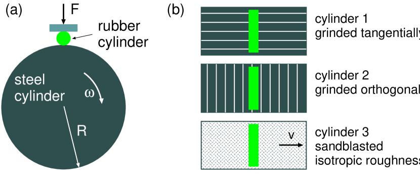
Figure 12: (a) Schematic picture of the experimental friction tester. The rubber cylinder is pushed with a dead weight towards the rotating steel cylinder. (b) The steel cylinder has surface roughness prepared by grinding the cylinder surface along the rotation direction (top), orthogonal to the rotation direction (middle) or by sandblasting (bottom). The latter results in surface roughness with isotropic statistical properties.

The experimental results, to be shown in in Sec. 5, were performed at a constant temperature of $20\pm 2^{\circ}\mathrm{C}$, whereas 5 different velocities are adopted in the present study ($2.5\leavevmode\nobreak\ \mathrm{mm/s}$, $4.5\leavevmode\nobreak\ \mathrm{mm/s}$, $8\leavevmode\nobreak\ \mathrm{mm/s}$, $14\leavevmode\nobreak\ \mathrm{mm/s}$ and $25\leavevmode\nobreak\ \mathrm{mm/s}$), as well as three different loads ($31.1$, $93.3$, and $155.5\leavevmode\nobreak\ \mathrm{N}$, corresponding to Hertz’s pressures ($\tilde{1}.2$, $2.1$, and $2.9\leavevmode\nobreak\ \mathrm{MPa}$) are applied for each velocity.

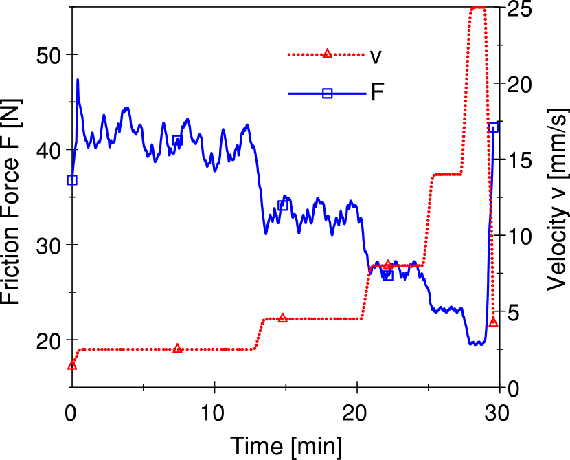
Figure 13: Friction force and velocity as a function of time during a typical experiment.

The test protocol, for each adopted rough surface (see in the following), is as follows. Under constant load, the sliding velocity is kept constant and friction measured during three cylinder revolutions before switching to the next velocity, leading to a total measurement time of about $30\leavevmode\nobreak\ \mathrm{min}$. This procedure is repeated three times using the same contact pair in order to detect possible running-in or wear effects of the seal. Afterward, a new seal and new load is used. The same lubricant is used during all experiments, however additional (repeated) experiments made at the end of the experimental campaign have confirmed that no measurable aging or contamination of the oil was occurring in the setup. An example chart showing the temporal evolution of the sliding speed, and corresponding measured friction force, is reported in Fig. 13.

Table 1: Normal load and maximum contact pressure (according to Hertz theory) during experiments.

Normal force (N)	Maximum cont. pressure (MPa)
31.1	1.2
93.3	2.1
155.5	2.9

4 Surface roughness power spectra

In all the experiments the contact consists of a steel cylinder with a rough surface, whereas the rubber can be considered smooth. Three cylinders with different surfaces were adopted. All the cylinder surfaces were first sandblasted to provide a statistically similar initial roughness. Next, the surfaces of two of the cylinders are grinded orthogonally (in the following, cylinder 2) or longitudinally (cylinder 1) to the sliding direction (perpendicular to the cylinder axis). A sketch of the surfaces is shown in Fig. 12(b). The surface roughness was measured at different positions along the azimuthal and meridian directions, through $20\leavevmode\nobreak\ \mathrm{mm}$ line-scans (eight scans for each surface). For the sandblasted cylinder $h_{\mathrm{rms}}\approx 1.0\leavevmode\nobreak\ \mathrm{\mu m}$, and for the surfaces with anisotropic roughness $h_{\mathrm{rms}}\approx 0.6\leavevmode\nobreak\ \mathrm{\mu m}$. The roughness is higher then recommended for a standard hydraulic cylinder rod, but is well suited for the investigation we provide in the following.

In the mean field theory it enters the two-dimensional (2D) power spectral density (PSD) $C(\mathbf{q})$ which can be calculated from the measured height profile $h(\mathbf{x})=h(x,y)$ using:

$$C\left(\mathbf{q}\right)=\left(2\pi\right)^{-2}\int d^{2}x\left\langle h\left(0\right)h\left(\mathbf{x}\right)\right\rangle e^{-i\mathbf{q}\cdot\mathbf{x}},$$

where the wave vector $q=(q_{x},q_{y})$, and where $h(\mathbf{x})$ is the surface roughness height at the point $\mathbf{x}=(x,y)$, with $\left\langle h\left(\mathbf{x}\right)\right\rangle=0$. However, (using a stylus profiler) we have only measured the topography $h=h(x)$ along a line, and in this case one can only calculate the one-dimensional power spectrum $C_{\mathrm{1D}}(q)$. For surfaces with isotropic roughness, $C_{\mathrm{2D}}\left(q\right)$ can be directly linked to line scans $C_{\mathrm{1D}}(q)$ usingCarbone2009

$$C_{\mathrm{2D}}\left(q\right)=-\int_{q}^{\infty}\frac{dk}{\pi}\leavevmode\nobreak\ {\frac{C_{\mathrm{1D}}^{\prime}(k)}{\sqrt{k^{2}-q^{2}}}}.$$

In Fig. 14, 15 and 16 we show, respectively, the calculated (averaged over 8 measurements repetitions) one dimensional surface roughness power spectra $C_{\mathrm{1D}}$ as a function of the wavenumber on log-log scale for cylinder 1 (longitudinal roughness), 2 (transverse roughness) and 3 (isotropic roughness). In the figures, the solid (red) and dashed (green) lines are, respectively, from line-scan along and perpendicular to the sliding direction. On the log-log scale, the PSDs are approximately linear for $q\gtrapprox 10^{5}\leavevmode\nobreak\ \mathrm{m}^{-1}$, and in particular the surfaces appear to be self affine fractal with the fractal dimension $D_{\mathrm{f}}=3-H\approx 2.2$, where $H$ denotes the Hurst exponent. Moreover, in Fig. 16 (isotropic roughness) we also show the 2D surface roughness power spectra, the latter calculated from the formula reported above. The solid blue lines indicate the slope of the corresponding self-affine region of the PSDs; they have been drawn displaced from experimental curves only for the sake of readability.

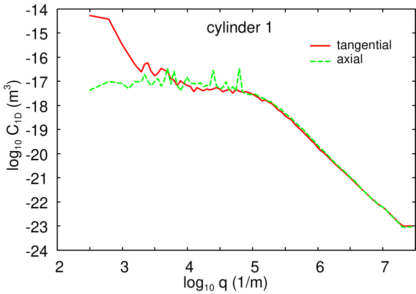
Figure 14: 1D surface roughness power spectra $C_{\mathrm{1D}}$ of cylinder surface 1 as a function of the wavenumber q; axial direction (dashed line) and the tangential direction (solid line).

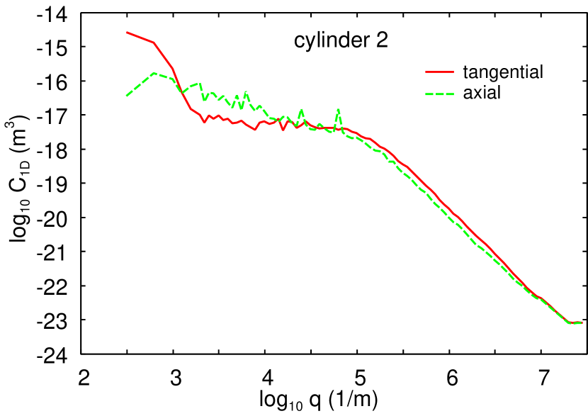
Figure 15: 1D surface roughness power spectra $C_{\mathrm{1D}}$ of cylinder surface 2 as a function of the wavenumber q; axial direction (dashed line) and the tangential direction (solid line).

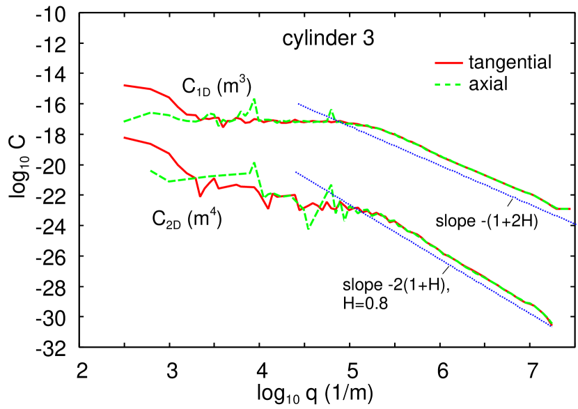
Figure 16: 1D and 2D surface roughness power spectra of cylinder surface 3 as a function of the wavenumber q along the axial direction (dashed line) and the tangential direction (solid line). The solid blue lines indicate the slope of the corresponding self-affine region of the PSDs; they have been drawn displaced from experimental curves only for the sake of readability.

5 Experimental results and discussion

5.1 Influence of squeezing load

In Fig. 17 we show for cylinder 2 (transverse roughness) the friction coefficient ${\mu}$ as a function of the sliding velocity $v_{0}$ for the three different loads. The plotted friction coefficient is the arithmetic mean of all corresponding measurements (error bars are not included in Fig. 17 for the sake of readability, but they will be included in the results following in this section).

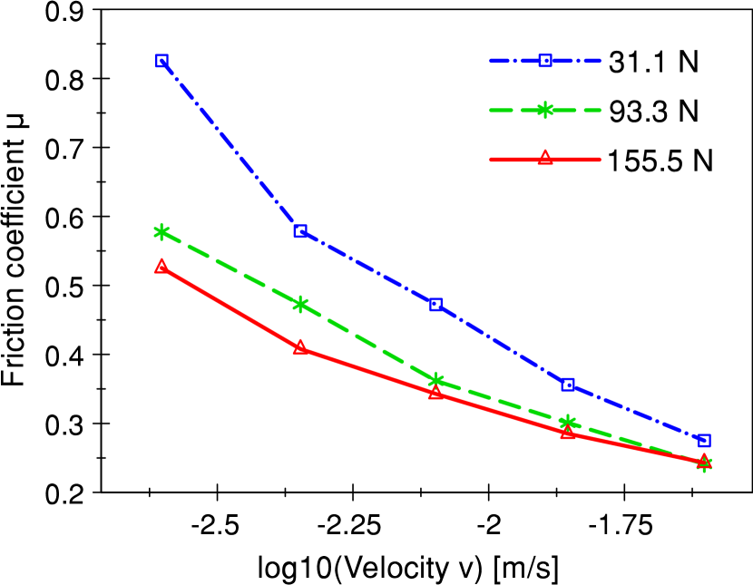
Figure 17: Friction coefficient $\mu$ as a function of the sliding velocity $v_{0}$ for all three normal loads. For cylinder 2 (transverse roughness).

Notice that the friction coefficient $\mu$ decreases as the velocity increases. Considering the adopted contact geometry and distribution of roughness and compliance on the solids, this behavior can be simply ascribed to the occurrence of the mixed lubrication regime in the contact. Furthermore, the friction coefficient decreases as the normal load increases. This too can be justified by observing that, in the mixed regime, part of the load is supported by the fluid-asperity interactions. Thus by, e.g., linearly increasing the load, the asperity contact area does not increase linearly with the load, and the tangential force, which is given by a a contact area term and a fluid shear term, increases less than linearly with increasing load, resulting in the lower friction coefficient (see Sec. 6).

5.2 Influence of the surface topography

Here we present the measured friction forces as a function of the sliding speed, for all three cylinders, at a normal load of $31.1\leavevmode\nobreak\ \mathrm{N}$ [Fig. 18(a)], $93.3\leavevmode\nobreak\ \mathrm{N}$ [Fig. 18(b)] and $155.5\leavevmode\nobreak\ \mathrm{N}$ [Fig. 18(c)].

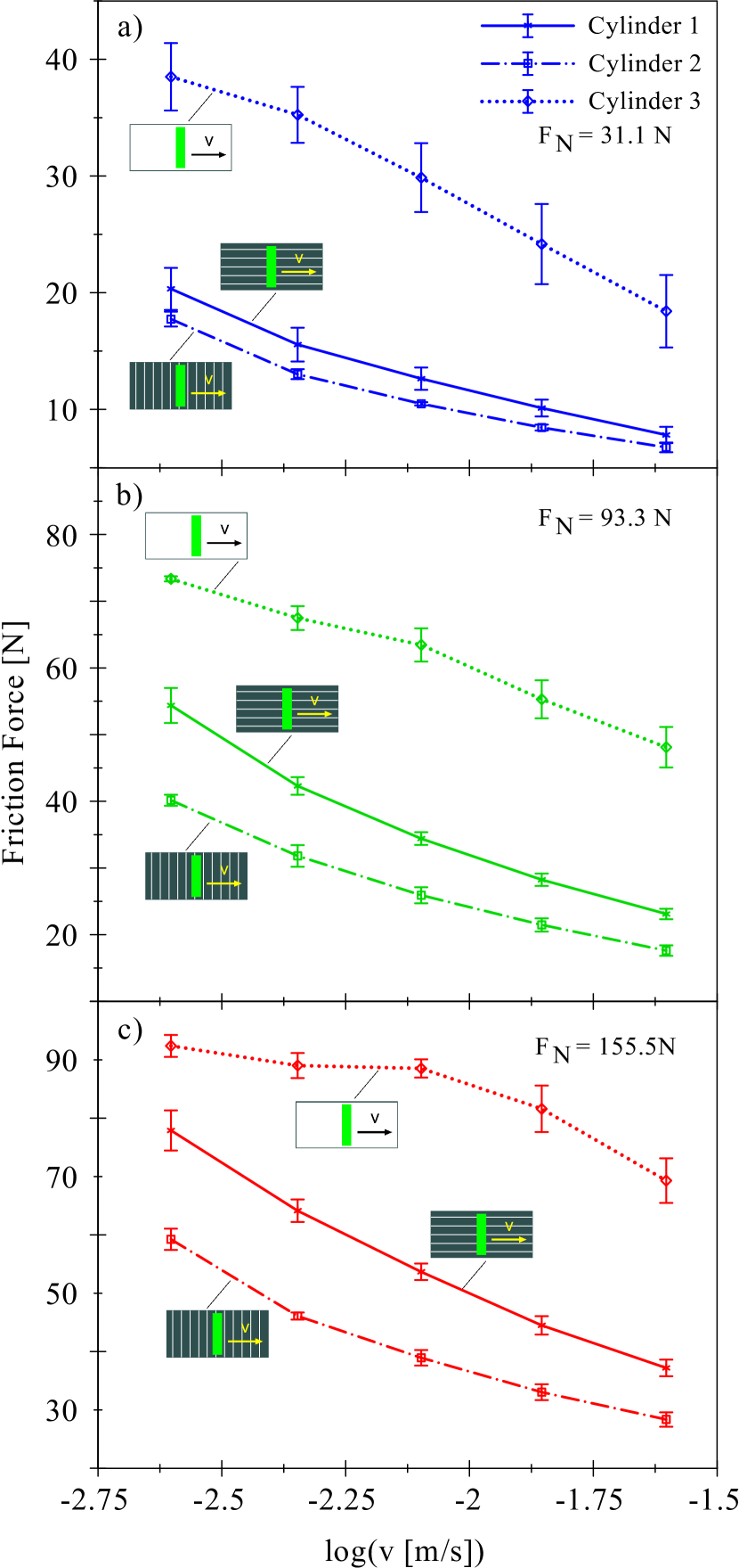
Figure 18: Friction forces as a function of the velocity $v$ (log scale), for all the test cylinders. Normal load (a) $31.1N$, (b) $93.3N$ and (c) $155.5N$.

The friction forces for cylinder 3 (isotropic roughness) are significantly higher, compared to the forces for cylinder 1 (longitudinal roughness) and 2 (transverse roughness). This is expected by the larger roughness, which makes the asperity-asperity interactions more important up to larger sliding velocities than for the lower roughness surfaces. Thus, at a same sliding speed, a larger solid contact area, and a larger solid contact friction, occurs for the rougher cylinder. We note that this is only true in the high velocity part of the mixed lubrication region, since in the boundary lubrication region the larger roughness result in smaller contact area and hence a smaller friction, at least if one can neglect the viscoelastic contribution to the friction (see Fig. 1 which illustrate this point).

It is interesting to compare the friction forces occurring for the contact case 1 and 2. In particular, the dissipation occurring for the cylinder with longitudinal roughness is always larger than for the transverse roughness. Considering that the rough surfaces show similar high (same Hurst exponent) and low (same root mean square roughness) frequency content, this must be due to the anisotropy of the surface. Indeed, as pointed out before, the grinding wear tracks along the sliding direction facilitate the removal of the fluid from the nominal contact region, and extend the boundary lubrication region to higher sliding speeds. In most cases this results in an increase in the friction force compared to the case of isotropic roughness with the same angular averaged power spectrum. In a similar way, when the grinding direction is orthogonal to the sliding direction, the fluid removal is reduced, resulting (in most cases) to lower friction than for isotropic roughness. This is also consistent with the results in Fig. 1 which in the high velocity part of the mixed lubrication part of the Stribeck curve show higher friction when sliding along the grinding direction.

The observation that the friction force of cylinder 1 is higher than the friction force of cylinder 2 applies to all investigated velocities and to all tested normal loads. Especially for the normal loads $93.3\leavevmode\nobreak\ \mathrm{N}$ and $155.5\leavevmode\nobreak\ \mathrm{N}$ the difference is significant. As the grinding direction is the only difference, the measured effect has to be caused by the anisotropic surfaces. In particular, the friction curves of cylinder 3, in the log-linear representation, show a negative curvature with respect to the (positive) curvature shown by the other surfaces.

At very low sliding speeds (in the boundary lubrication region) it is likely that the friction force is biggest when the grinding direction is orthogonal to the sliding direction. This is the case because fluid hydrodynamic effects are not important at very low sliding speed. At the same time there may be a viscoelastic contribution to the friction which will be largest when sliding orthogonal to the grinding direction (see discussion around Fig. 1); with the present experimental set-up we where not able to study the friction in the boundary lubrication velocity range.

To summarize, the friction asymmetry exhibited in Fig. 18 is related to the anisotropy of the adopted surface roughness, where surface 1 has a main scratch direction which is aligned with the sliding direction. This configuration has been shown in the literature to provide the smallest fluid-asperity interaction contribution ([12], [13], [15] and [16]): roughly speaking, the fluid is allowed to escape along the roughness channels (through the scratch valleys) without generate a strong fluid overpressure. Thus, the total fluid pressure is almost negligible, resulting in a larger amount of asperity-asperity interactions. This finally results in a Stribeck curve which occurs closer to the boundary-mixed regime, the latter typically characterized by a negative curvature. The opposite holds for the surfaces 2 and 3 where, instead, the fluid-asperity interaction is higher, allowing to displace the Stribeck curve toward the mixed-hydrodynamic regime, where the curvature is typically positive. This is in perfect agreement with the results also shown in Fig. 20.

5.3 Discussion

The experiments show a distinct influence of the surface topography, especially when comparing the two anisotropic surfaces 1 and 2. Two effects do contribute to the friction process.

i) The fluid-asperity interactions occurring when the sliding direction is perpendicular to the grooves main direction (so called transverse roughness) is typically stronger than for the aligned grooves (longitudinal roughness), when the groove representative size is smaller than the smallest nominal contact length. This is well known in the literature of mixed lubrication for soft contacts [11, 12] and of hydrodynamic lubrication for textured surfaces [13, 14]. Thus, a larger asperity-induced fluid pressure is provided for the transverse roughness, which in turn determines an increased average interfacial separation (resulting from the decrease of the solid-solid contact pressure) and, therefore, a reduced dry contact area. However, in term of the resulting fluid viscous dissipation, this stronger fluid-asperity interaction for the transverse roughness can cause both an increase or decrease of the total friction, depending on the range of sliding velocity at which this interaction dominates. Thus, in the present case the stronger fluid-asperity interaction (for the transverse roughness range) only determines a reduction of the dry-contact friction (due to the decrease of the contact area), whereas the fluid-viscous dissipation occurring at the asperity scale (micro-EHL) seems not to dominate this mixed lubrication contact configuration (as a counter example, see Ref. [15]).

ii) The reduced dry (or boundary lubricated) contact area suggested in i) determines, consequently, a reduction of the friction contributions coming from the intimate (or boundary mediated) asperity-asperity interaction. In particular, the solid-contact friction can originate, in the present case, by both the adhesive contribution (proportional to the dry true contact area) and by the micro-rolling contribution (a dissipation originating by the pulsating deformation on the rubber seal by the sliding asperities) [16]. For small true contact areas (of interest for the seal application), and depending on the sliding speed, the hysteretic contribution to friction is slightly dependent on the contact area. Thus, the decrease of dry contact obtained for the transverse roughness does induce a decrease of dry friction, resulting in the overall friction decrease with respect to the longitudinal roughness.

6 Theory analysis

In this section we will analyze the experimental results presented above. The friction coefficient as a function of sliding speed for the lubricated contact, the so called Stribeck curve, will be calculated. We will discuss in detail how the surface roughness influences the Stribeck curve, and in particular under which conditions it will shift the Stribeck curve to lower sliding speeds as this reduces the friction and the wear of the rubber seal. As input for the calculation, the surface roughness power spectra of the surfaces involved (Figures 14, 15 and 16), and the effective elastic modulus of the solids are needed. In the study below the surface roughness on the rubber surface will be neglected, and only the roughness of the steel cylinders is considered.

Due to the incomplete experimental information about the surface roughness anisotropy, and the absence of information about the frictional properties of the dry rubber-countersurface contacts, in particular how the frictional shear stress in the area of real contact depends on the sliding speed, the present study is only of semi-quantitative nature. Nevertheless, the origin of the observed dependency of the friction coefficient on the load and the influence of the surface roughness anisotropy on the friction will be explained. The anisotropy of surface roughness can be characterized by the Tripp number. Roughly speaking, the Tripp number is the ratio $\gamma=\xi_{x}$/$\xi_{y}$ between the axis of the elliptic cross-section (in the $xy$-plane) of an (average) asperity in real $(x,y)$ space. In fluid dynamics, the Tripp number is the quantity which naturally appears in the fluid flow equations. The Tripp number can be easily obtained from the 2D surface roughness power spectrum $C(q_{x},q_{y})$, see Ref. [17, 11]. Thus, to determine the Tripp number accurately, topography measurements over surface areas rather than 1D line-scans are necessary. It is clear, however, that in the present case, because of the preparation method, surface 3 has the Tripp number $\gamma=1$, while surface 2 has $\gamma<1$. Since surface 1 is ground orthogonal to the cylinder axis, i.e., along the sliding direction, it must have $\gamma>1$ but Fig. 14 shows it must be very close to one as nearly no difference occurs in the 1D power spectra along the two directions.

For a complete and accurate analysis one need in general the surface roughness power spectra for all wavenumbers, i.e., down to atomic distances corresponding to wavenumbers $q\approx 10^{10}\leavevmode\nobreak\ \mathrm{m}^{-1}$, or wavelength of order $\mathrm{nm}$, which requires studying the surface roughness with (near) atomic resolution, using, e.g., Atomic Force Microscopy (AFM). However, it will be shown below that the velocity and load dependency of the friction force in the present case is due mainly to the influence of the longest wavelength roughness components on the fluid dynamics. The large wavenumber cut-off $q_{1}$ is chosen so that the surface root mean square slope equal 1.3, when including all the roughness with wavenumber $q<q_{1}$. The results presented below are not sensitive to this assumption.

For the mixed-elastohydrodynamic calculations presented below the elastic properties of the solids are needed. The steel cylinders will be treated as rigid. Rubber is a viscoelastic material which can be characterized by a viscoelastic modulus $E\left(\omega\right)$ which depends on the frequency $\omega$ with which it is deformed. Note that $E\left(\omega\right)$ is a complex quantity, where the imaginary part is associated with energy dissipation, resulting from the friction force which acts between the rubber chain molecules when they slip relative to each other. For lubricated sliding friction the viscoelasticity of the rubber will also contribute to the friction in the area of contact. However, in the present study this will not be considered in detail but it will just be assumed that a constant frictional shear stress $\tau_{1}$ acts in the area of real contact (see also discussion below). Now, when the rubber cylinder slides on the steel counter surface there will be two types of deformations. First, there will be a macroscopic Hertz’s-like deformation of the rubber cylinder. This deformation is constant in time so it is determined by the low frequency modulus of the rubber which was measured (including non-linearity effects) to be about $E\approx 9\leavevmode\nobreak\ \mathrm{MPa}$. However, the true area of contact is determined by the interaction between the asperities on the steel surface and the rubber. During sliding this includes high-frequency deformations involving a band of deformation frequencies $\omega\approx qv$, where $q=2\pi/\lambda$ is the wavenumber (and $\lambda$ the wavelength) of a surface roughness component, and $v$ the sliding speed. This will result in a stiffening of the rubber with increasing sliding speed, and to a contact area $A(v)$ which, even for dry contact, decreases with increasing sliding speed. In this study this effect will not be included but it is assumed that in the boundary lubrication region $A\left(v\right)\tau\left(v\right)$, i.e. the adhesive contribution to friction, is a constant. Thus, the only velocity (and load) dependency in the figures presented below is due the fluid dynamics. In reality, this may not hold accurately, but it is likely that the strong velocity dependence observed in a relative narrow (mixed lubrication) velocity region, is due mainly to fluid dynamics effects.

We now consider the sliding of an elastic cylinder on the hard, lubricated counter surface with random roughness. First the friction for cylinder 3 is considered, which has surface roughness with isotropic statistical properties. Fig. 19 shows the fluid pressure and shear stress flow factors, $\phi_{\mathrm{p}}$ and $\phi_{\mathrm{s}}$, as a function of the surface separation $\bar{u}$, as obtained using the theory of Ref. [14]. Note that for isotropic roughness $\phi_{\mathrm{p}}<1$, and since the pressure flow factor appears together with the viscosity in the combination $\eta_{\mathrm{eff}}=\eta/\phi_{\mathrm{p}}>\eta$, it follows that the fluid pressure flow factor will shift the mixed lubrication region towards lower sliding speed, as well as increase the strength of the generic fluid-asperity interaction given the larger effective viscosity. When the surface roughness occurs on the moving substrate surface, as in the present case, the fluid shear stress flow factor $\phi_{\mathrm{s}}$ is positive, and according to Eq. (2) this will result in a shift of the Stribeck curve towards lower sliding speed. The physical reason for this is as follows: consider the rough substrate surface moving against the smooth elastic cylinder. The fluid carried in the valleys of the moving rough surface helps to transport fluid from the leading edge into the gap, and hence support fluid lubrication, and shift the Stribeck curve towards lower sliding speed.

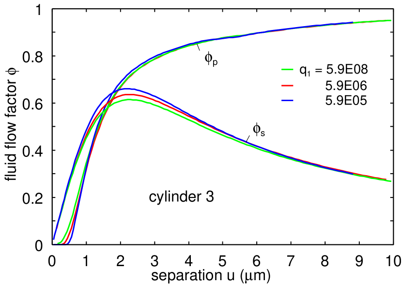
Figure 19: The fluid pressure flow factor $\phi_{P}$ and shear stress flow factor $\phi_{s}$ as a function of the surface separation using the surface roughness power spectrum of cylinder 3 with three different large wavenumber cut-off: $q_{1}=5.9\leavevmode\nobreak\ 10^{8}$, $q_{1}=5.9\leavevmode\nobreak\ 10^{6}$ and $q_{1}=5.9\leavevmode\nobreak\ 10^{8}$ $m^{-1}$.

A very important observation for what follows is that unless the contact pressure is very high, the flow factors are mainly determined by the most long-wavelength part of the surface roughness. This is illustrated in Fig. 19 where the flow factors for three different large wavenumber cut-off $q_{1}$ are shown. Note the relative small difference between the three cases in spite of the large variation (by three decades in length scale) in the cut-off $q_{1}$. The reason for this is that the long-wavelength (and large amplitude) surface roughness components generate the biggest fluid flow channels at the interface, and will hence influence the fluid flow dynamics at the interface much stronger than the smaller channels arising from the shorter surface roughness components. At very high contact pressures this is no longer the case, but for the present situation it holds to a very good approximation.

To obtain the Stribeck curve for cylinder 3, information about the frictional shear stress acting in the area of real contact is needed. For rubber sliding on dry hard rough surfaces the friction coefficient is usually nearly independent of the nominal contact pressure [7]. In particular, the frictional shear stress $\tau$ acting in the area of real contact is independent of the local contact pressure in the pressure range relevant in most applications involving rubber materials. For lubricated surfaces it was found above that the friction coefficient depends strongly on the load. In the hydrodynamic region for smooth surfaces the Stribeck curve depends on $\eta v/F_{\mathrm{n}}$ but this scaling is not valid in the mixed lubrication region. In Fig. 20 the relation between the friction coefficient and the sliding speed for cylinder 3 and for the three different loads used in the experiments reported on above are shown. In the calculations was assumed that a (velocity independent) frictional shear stress $\tau_{1}=13.5\leavevmode\nobreak\ \mathrm{MPa}$ acts in the area of real contact.

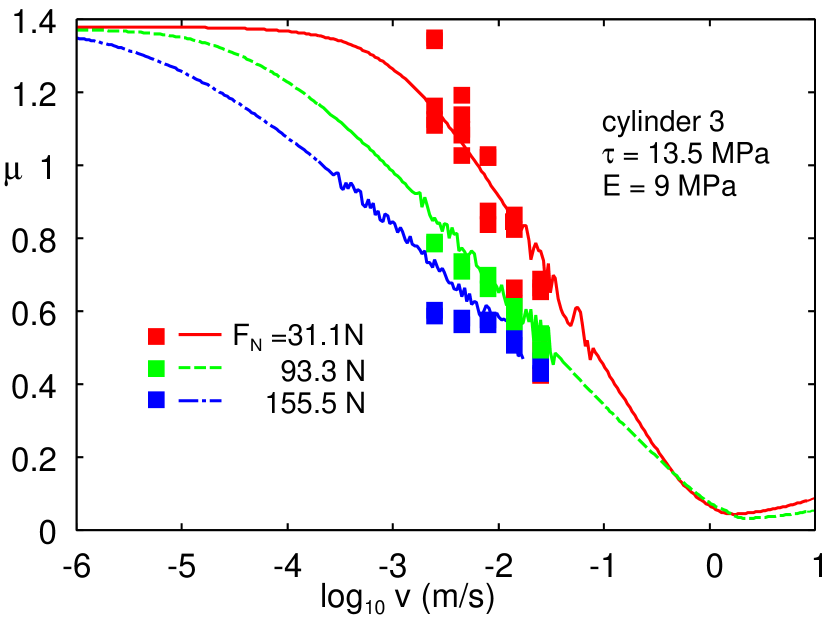
Figure 20: The calculated (solid lines) and measured friction coefficients as a function of sliding speed for three different loads, $F_{\mathrm{N}}$ = 31.1, 93.3 and 155.5 N.

Note that the friction coefficient depends on the load, in relative good agreement with the experimental data (square symbols). Due to a numerical instability, for the highest load the calculated results terminates before reaching the highest sliding speed. As pointed out above, unless the contact pressure is very large (resulting in very small interfacial separation), the fluid flow factors depend mainly on the longest wavelength roughness components. However, the area of real contact depends on all the roughness wavelength components and decreases continuously as the large wavenumber cut-off $q_{1}$ increases. In the boundary lubrication region all the load is carried by the area of real contact $A$ and in this case in our model the friction force $F_{\mathrm{f}}=A\tau$ (note: in reality, in the boundary lubrication velocity range there will also be a viscoelastic contribution to the friction from the time-dependent deformations of the rubber surface by the asperities of the countersurface). In Fig. 21 the Stribeck curves for cylinder 3 are shown, using three different large wavenumber cut-off $q_{1}$ but adjusting the frictional shear stress so the friction force in the boundary lubrication region is (nearly) the same in all cases. Note that in this case the Stribeck curves are nearly identical. This is the case only because the fluid flow factors are mainly determined by the most long-wavelength part of the surface roughness spectra, which is the same in all cases.

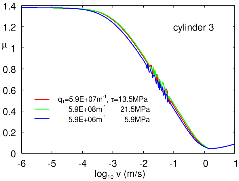
Figure 21: The calculated friction coefficients as a function of sliding speed for the load $F_{\mathrm{N}}$ = 31.1 N for several different large wavenumber cut-off q1.

We now consider the rubber friction for cylinder 2. For this case the fluid flow factors for three different cases are calculated, namely isotropic roughness (corresponding to the Tripp number $\gamma=1$), and for anisotropic roughness with the grinding groves along the sliding direction (corresponding to the Tripp number $\gamma=8$), and with the grinding direction orthogonal to the sliding direction (corresponding to the Tripp number $\gamma=1/8$) as in the actual system. Fig. 22 and 23 show the fluid flow and shear stress flow factors for all three cases, respectively.

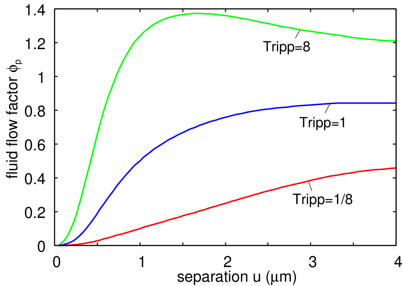
Figure 22: The fluid pressure flow factor $\phi_{P}$ as a function of the average separation u for cylinder 2 assuming the Tripp asymmetry number $\gamma$ = 1, 8 and 1/8.

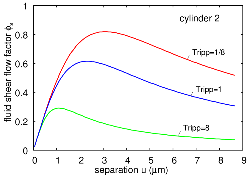
Figure 23: The fluid shear stress flow factor $\phi_{S}$ as a function of the average separation u for cylinder 2 assuming the Tripp asymmetry number $\gamma$ = 1, 8 and 1/8.

Note that for $\gamma=8$, for the surface separation $\bar{u}>1\leavevmode\nobreak\ \mathrm{\mu m}$ the fluid flow factor $\phi_{\mathrm{p}}>1$, which would shift the Stribeck curve towards higher sliding speeds. However, in the studied velocity range the interfacial separation is smaller than $0.6\leavevmode\nobreak\ \mathrm{\mu m}$, in which case the pressure flow factor is smaller than 1 (see Fig. 22). As a result the fluid pressure flow factor will shift the Stribeck curve to lower sliding speeds. Similarly, the shear stress flow factor shifts the Stribeck curve towards lower sliding speeds. For the surface with the grinding direction orthogonal to the sliding direction (which is the actual case for cylinder 2), $\gamma=1/8$, $\phi_{\mathrm{p}}<1$ for all interfacial separations, and both the pressure and shear stress flow factors shift the Stribeck curve towards lower sliding speed, see Fig. 24. Fig. 24 also show the calculated Stribeck curve for the cylinder 3 is shown (experimental data from Fig. 20).

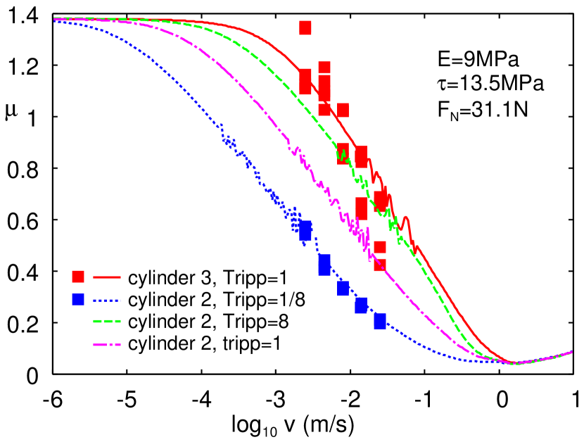
Figure 24: The calculated (solid lines) and measured friction coefficients as a function of sliding speed for the load $F_{\mathrm{N}}$ = 31.1 N.

Note that in the studied velocity interval the friction for cylinder 3 is larger than for cylinder 2, which is due to the larger roughness on cylinder 3, and also due to the difference in the surface roughness anisotropy, both of which result in faster fluid squeeze-out for cylinder 3.

7 Summary and conclusions

In this paper we have presented a combined experimental-theoretical investigation of the influence of anisotropic surfaces on the friction behavior of a hard-soft contacts. We have discussed in detail how the fluid flow and friction shear stress factors depend on the surface roughness. A test rig was described, which is designed to investigate a soft, lubricated line contact in detail. An O-ring cord is brought into contact with the lateral surface of an uniformly rotating steel cylinder. Three cylinders with different surfaces are used: One sandblasted isotropic surface and two anisotropic surfaces, grooved orthogonal or longitudinal to the direction of motion. A distinct influence of anisotropic surfaces is detected. The friction force decreases when the surface is grooved perpendicular to the direction of motion. Finally, the experimental results were compared with calculations. These experimental results clearly show that the anisotropy of surfaces in engineering applications has to be considered when modeling lubricated friction of hydraulic seals.

Appendix A

Here we show how to calculate the rolling friction (both micro- and macro-contributions) coming from the solid contact. We first observe that the following contact relation applies

$$p_{\mathrm{cont}}\left(\mathbf{x}\right)\nabla u\left(\mathbf{x}\right)=0,$$

leading to the equality

$$p_{\mathrm{cont}}\left(\mathbf{x}\right)\nabla u^{\mathrm{top}}\left(\mathbf{x}\right)=p_{\mathrm{cont}}\left(\mathbf{x}\right)\nabla u^{\mathrm{down}}\left(\mathbf{x}\right),$$

where $u^{\mathrm{top}}\left(\mathbf{x}\right)$ and $u^{\mathrm{down}}\left(\mathbf{x}\right)$ correspond to the top- and down-body surface, respectively. $p_{\mathrm{cont}}\left(\mathbf{x}\right)\nabla u^{\mathrm{down}}\left(\mathbf{x}\right)$ provides on the bottom solid (same but with minus sign on the upper solid) the tangential component of the locally-applied solid contact pressure, which contributes to the total measured sliding friction. We are interested in the ensemble average $\left\langle p_{\mathrm{cont}}\left(\mathbf{x}\right)\nabla u^{\mathrm{down}}\left(\mathbf{x}\right)\right\rangle$ which reads

$$\left\langle p_{\mathrm{cont}}\left(\mathbf{x}\right)\nabla u^{\mathrm{down}}\left(\mathbf{x}\right)\right\rangle=\frac{A_{\mathrm{c}}}{A_{0}}\left\langle p_{\mathrm{cont}}\left(\mathbf{x}\right)\nabla u^{\mathrm{down}}\left(\mathbf{x}\right)\right\rangle_{A_{\mathrm{c}}},$$

where $\left\langle{}\right\rangle_{A_{\mathrm{c}}}$ is the ensemble average provided on the solid contact domain. We write

$$\left\langle p_{\mathrm{cont}}\left(\mathbf{x}\right)\nabla u^{\mathrm{down}}\left(\mathbf{x}\right)\right\rangle_{A_{\mathrm{c}}}=\frac{\bar{p}_{\mathrm{cont}}\left(\mathbf{x}\right)}{A_{\mathrm{c}}/A_{0}}\left\langle\nabla u^{\mathrm{down}}\left(\mathbf{x}\right)\right\rangle_{A_{\mathrm{c}}}+\left\langle p_{1,\mathrm{cont}}\left(\mathbf{x}\right)\nabla u_{1}^{\mathrm{down}}\left(\mathbf{x}\right)\right\rangle_{A_{\mathrm{c}}},$$

$\frac{A_{\mathrm{c}}}{A_{0}}\left\langle p_{1,\mathrm{cont}}\left(\mathbf{x}\right)\nabla u_{1}^{\mathrm{down}}\left(\mathbf{x}\right)\right\rangle_{A_{\mathrm{c}}}=\left\langle p_{1,\mathrm{cont}}\left(\mathbf{x}\right)\nabla u_{1}^{\mathrm{down}}\left(\mathbf{x}\right)\right\rangle$ is the micro-rolling friction (to be calculated as shown in Ref. XX), whereas $\bar{p}_{\mathrm{cont}}\left(\mathbf{x}\right)\left\langle\nabla u^{\mathrm{down}}\left(\mathbf{x}\right)\right\rangle_{A_{\mathrm{c}}}$ is the macro-rolling friction. In (10a) and (10b) the term $\left\langle p_{1,\mathrm{cont}}\left(\mathbf{x}\right)\nabla u_{1}^{\mathrm{down}}\left(\mathbf{x}\right)\right\rangle$ is implicitly included in the true shear stress $\tau_{1}$.

Note that $\left\langle u^{\mathrm{down}}\left(\mathbf{x}\right)\right\rangle_{A_{\mathrm{c}}}$ corresponds to the average contact plane. $\left\langle u^{\mathrm{down}}\left(\mathbf{x}\right)\right\rangle_{A_{\mathrm{c}}}$ is thus given by $\bar{u}^{\mathrm{down}}\left(\mathbf{x}\right)+\bar{u}_{\mathrm{cp}}^{\mathrm{down}}\left(\mathbf{x}\right)$, where $\bar{u}_{\mathrm{cp}}^{\mathrm{down}}$ is the average separation separating the average bottom solid surface $\bar{u}^{\mathrm{down}}\left(\mathbf{x}\right)$ from the average contact plane$\left\langle u^{\mathrm{down}}\left(\mathbf{x}\right)\right\rangle_{A_{\mathrm{c}}}$. Note that $\bar{u}_{\mathrm{cp}}^{\mathrm{down}}\left(\mathbf{x}\right)+\bar{u}_{\mathrm{cp}}^{\mathrm{up}}\left(\mathbf{x}\right)=\bar{u}\left(\mathbf{x}\right)$, where $\bar{u}_{\mathrm{cp}}^{\mathrm{up}}$ is the average separation separating the average upper solid surface $\bar{u}^{\mathrm{up}}\left(\mathbf{x}\right)$ from the average contact plane$\left\langle u^{\mathrm{up}}\left(\mathbf{x}\right)\right\rangle_{A_{\mathrm{c}}}$, given that $\left\langle u^{\mathrm{down}}\left(\mathbf{x}\right)\right\rangle_{A_{\mathrm{c}}}=\left\langle u^{\mathrm{up}}\left(\mathbf{x}\right)\right\rangle_{A_{\mathrm{c}}}$. To calculate the macro-rolling friction we thus need to calculate $\bar{u}_{\mathrm{cp}}^{\mathrm{down}}\left(\mathbf{x}\right)$ (or $\bar{u}_{\mathrm{cp}}^{\mathrm{up}}\left(\mathbf{x}\right)$). We do this in an approximated way as follows. In particular, we consider the variation $d\bar{u}_{\mathrm{cp}}^{\mathrm{down}}\left(\mathbf{x}\right)$ as due to a variation of the average applied solid contact pressure $\sigma_{0}$

$$d\bar{u}_{\mathrm{cp}}^{\mathrm{down}}\left(\mathbf{x}\right)=\frac{1}{A_{\mathrm{c}}}\sum_{i}dA_{\mathrm{c}i}du_{i,\mathrm{cp}}^{\mathrm{down}},$$

where we have adopted $\left\langle{}\right\rangle_{A_{\mathrm{c}}}=A_{\mathrm{c}}^{-1}\sum_{i}dA_{\mathrm{c}i}$ for homogeneous processes, and where $dA_{\mathrm{c}i}$ is representative of the i-th asperity contact area. Since $du_{i,\mathrm{cp}}^{\mathrm{down}}=-dw_{i}^{\mathrm{down}}$, where $dw_{i}^{\mathrm{down}}$ is the local variation of displacement field, we thus write

$$d\bar{u}_{\mathrm{cp}}^{\mathrm{down}}\left(\mathbf{x}\right)=-\frac{1}{A_{\mathrm{c}}}\sum_{i}dA_{\mathrm{c}i}dw_{i}^{\mathrm{down}}.$$

By considering that, for practical applications, the average effective solid pressure acting in the generic i-th asperity contact area $\sigma_{i}$ is almost constantly valued (i.e. not dependent on the externally applied load, unless for very large contact areas), we can write

$$\frac{1}{A_{\mathrm{c}}}\sum_{i}dA_{\mathrm{c}i}dw_{i}^{\mathrm{down}}\approx\frac{1}{A_{0}\sigma_{0}}\sum_{i}dA_{\mathrm{c}i}\sigma_{i}dw_{i}^{\mathrm{down}}=\frac{1}{A_{0}\sigma_{0}}dU_{\mathrm{el}}^{\mathrm{down}}\left(\mathbf{x}\right),$$

where $dU_{\mathrm{el}}^{\mathrm{down}}$ is the interfacial elastic energy stored in the bottom solid. Therefore, the following differential relation applies in the linear solid contact regime

$$d\bar{u}_{\mathrm{cp}}^{\mathrm{down}}A_{0}\sigma_{0}=-dU_{\mathrm{el}}^{\mathrm{down}}.$$

Upon integrating the previous equation, and for the case of elastic contact where only one of the solids is rough, one can relatively easily show that

$$\bar{u}_{\mathrm{cp}}^{\mathrm{down}}\left(\mathbf{x}\right) =\bar{u}\left(\mathbf{x}\right)\frac{E_{\mathrm{r}}^{\mathrm{up}}}{E_{\mathrm{r}}^{\mathrm{down}}+E_{\mathrm{r}}^{\mathrm{up}}}$$

$$\bar{u}_{\mathrm{cp}}^{\mathrm{up}}\left(\mathbf{x}\right) =\bar{u}\left(\mathbf{x}\right)\frac{E_{\mathrm{r}}^{\mathrm{down}}}{E_{\mathrm{r}}^{\mathrm{down}}+E_{\mathrm{r}}^{\mathrm{up}}}.$$

Therefore, the macro-rolling solid friction term reads for the upper solid

$$-\bar{p}_{\mathrm{cont}}(x,t)\left[\nabla\bar{u}^{\mathrm{up}}(x,t)-\nabla\bar{u}(x,t)\frac{E_{\mathrm{r}}^{\mathrm{down}}}{E_{\mathrm{r}}^{\mathrm{down}}+E_{\mathrm{r}}^{\mathrm{up}}}\right]$$

and for the lower solid

$$\bar{p}_{\mathrm{cont}}(x,t)\left[\nabla\bar{u}^{\mathrm{down}}(x,t)+\nabla\bar{u}(x,t)\frac{E_{\mathrm{r}}^{\mathrm{up}}}{E_{\mathrm{r}}^{\mathrm{down}}+E_{\mathrm{r}}^{\mathrm{up}}}\right],$$

where

$$\nabla\bar{u}^{\mathrm{up}}(x,t)-\nabla\bar{u}(x,t)\frac{E_{\mathrm{r}}^{\mathrm{down}}}{E_{\mathrm{r}}^{\mathrm{down}}+E_{\mathrm{r}}^{\mathrm{up}}}=\nabla\bar{u}^{\mathrm{down}}(x,t)+\nabla\bar{u}(x,t)\frac{E_{\mathrm{r}}^{\mathrm{up}}}{E_{\mathrm{r}}^{\mathrm{down}}+E_{\mathrm{r}}^{\mathrm{up}}}.$$

Appendix B

In this section we describe how to calculate the frictional correction factors for the generic contact case where the roughness is included only on one of the two contact surfaces. The most general case where both surfaces are rough has been described by some of us in a recent paper MS4 ; MS3 by using a different homogenization procedure than used here. In a near future the authors will provide a unified homogenization framework for the most general wet contact case.

In Ref. MS2 we show how to calculate $\left\langle u\nabla p\right\rangle$ in the low contact pressure regime $\bar{u}\gg h_{rms}$ and high contact pressure regime $\bar{u}\ll\bar{u}_{c}$. We summarize here the main effective equations:

For the case where the rough surface is fixed MS2 :

$$\bar{u}\gg h_{\mathrm{rms}} : \left\langle u\nabla p\right\rangle=a_{1}\bar{u}\nabla\bar{p}+a_{2}\frac{2\mathbf{v}_{0}\eta_{0}}{\bar{u}}$$ (1)

$$\bar{u}\ll\bar{u}_{\mathrm{c}} : \left\langle u\nabla p\right\rangle=3\bar{u}\left\langle\frac{1}{u}\right\rangle\frac{2v_{0}\eta}{\bar{u}},$$ (2)

corresponding, respectively, to (16) and (17) and leading to an effective flow

$$J_{0}=-\phi_{\mathrm{p}}\frac{\bar{u}^{3}}{12\eta}\nabla\bar{p}+\frac{1}{2}\phi_{\mathrm{s}}h_{\mathrm{rms}}v_{0}+\frac{1}{2}\bar{u}v_{0}.$$

For the case where the rough surface is sliding:

Using the same procedure as in Ref. MS2 one we obtain

$$\bar{u}\gg h_{\mathrm{rms}} : \left\langle u\nabla p\right\rangle=a_{1}\bar{u}\nabla\bar{p}-a_{2}\frac{2\mathbf{v}_{0}\eta_{0}}{\bar{u}}$$ (3)

$$\bar{u}\ll\bar{u}_{\mathrm{c}} : \left\langle u\nabla p\right\rangle=-3\bar{u}\left\langle\frac{1}{u}\right\rangle\frac{2v_{0}\eta}{\bar{u}},$$ (4)

leading to an effective flow

$$J_{0}=-\phi_{\mathrm{p}}\frac{\bar{u}^{3}}{12\eta}\nabla\bar{p}-\frac{1}{2}\phi_{\mathrm{s}}h_{\mathrm{rms}}v_{0}+\frac{1}{2}\bar{u}v_{0}.$$

In (1) to (4) we have

$$a_{1} = \left(1-\langle h^{2}\rangle D{\frac{3}{\bar{u}^{2}}}\right)$$

$$a_{2} = 3D\frac{\langle h^{2}\rangle}{u^{2}}.$$

We now consider the effective frictional stresses. We write the separation, at first order, as

$$u\left(\mathbf{x}\right)=\bar{u}\left(\mathbf{x}\right)+u_{1}^{\mathrm{up}}\left(\mathbf{x}\right)+u_{1}^{\mathrm{down}}\left(\mathbf{x}\right),$$

where $u_{1}^{\mathrm{up}}\left(\mathbf{x}\right)=w_{1}^{\mathrm{up}}\left(\mathbf{x}\right)-h^{\mathrm{up}}\left(\mathbf{x}\right)$ and $u_{1}^{\mathrm{down}}\left(\mathbf{x}\right)=w_{1}^{\mathrm{down}}\left(\mathbf{x}\right)-h^{\mathrm{down}}\left(\mathbf{x}\right)$, where $w_{1}^{\mathrm{\cdot}}$ is the first order surface displacement field (positive when inward the solid) and $h^{\mathrm{\cdot}}$ is the surface roughness. Furthermore, we define the deformed locally averaged solids profile as $\bar{u}^{\mathrm{up}}\left(\mathbf{x}\right)$ and $\bar{u}^{\mathrm{down}}\left(\mathbf{x}\right)$, with $\bar{u}\left(\mathbf{x}\right)=\bar{u}^{\mathrm{up}}\left(\mathbf{x}\right)-\bar{u}^{\mathrm{down}}\left(\mathbf{x}\right)$ (see also in the main text). In this work we only consider the case where $h^{\mathrm{up}}\left(\mathbf{x}\right)=0$ or $h^{\mathrm{down}}\left(\mathbf{x}\right)=0$.
a) Upper surface fixed - lower surface sliding
In this case, the frictional shear stress acting on the upper surface is

$$\tau_{\mathrm{fluid}}^{\mathrm{up}}\left(\mathbf{x}\right)=\frac{\eta v_{0}}{u\left(\mathbf{x}\right)}-\frac{1}{2}u\left(\mathbf{x}\right)\nabla p\left(\mathbf{x}\right)-p\left(\mathbf{x}\right)\nabla\left(\bar{u}^{\mathrm{up}}\left(\mathbf{x}\right)+u_{1}^{\mathrm{up}}\left(\mathbf{x}\right)\right),$$

whereas on the lower surface

$$\tau_{\mathrm{fluid}}^{\mathrm{down}}\left(\mathbf{x}\right)=-\frac{\eta v_{0}}{u\left(\mathbf{x}\right)}-\frac{1}{2}u\left(\mathbf{x}\right)\nabla p\left(\mathbf{x}\right)+p\left(\mathbf{x}\right)\nabla\left(\bar{u}^{\mathrm{down}}\left(\mathbf{x}\right)-u_{1}^{\mathrm{down}}\left(\mathbf{x}\right)\right).$$

After some manipulation one gets

$$\left\langle\tau_{\mathrm{fluid}}^{\mathrm{up}}\left(\mathbf{x}\right)\right\rangle = \bar{\tau}_{\mathrm{visc}}^{\mathrm{up}}\left(\mathbf{x}\right)-\bar{p}\nabla\bar{u}^{\mathrm{up}}$$ (5)

$$\bar{\tau}_{\mathrm{visc}}^{\mathrm{up}}\left(\mathbf{x}\right) = \left(v_{0}\left\langle\frac{\eta}{u}\right\rangle+\frac{1}{2}\left\langle u\nabla p\right\rangle-\left\langle u_{1}^{\mathrm{down}}\nabla p_{1}\right\rangle\right)-\bar{u}\nabla\bar{p}$$ (6)

and

$$\left\langle\tau_{\mathrm{fluid}}^{\mathrm{down}}\left(\mathbf{x}\right)\right\rangle = \bar{\tau}_{\mathrm{visc}}^{\mathrm{down}}\left(\mathbf{x}\right)+\bar{p}\nabla\bar{u}^{\mathrm{down}}$$ (7)

$$\bar{\tau}_{\mathrm{visc}}^{\mathrm{down}}\left(\mathbf{x}\right) = -\left(v_{0}\left\langle\frac{\eta}{u}\right\rangle+\frac{1}{2}\left\langle u\nabla p\right\rangle-\left\langle u_{1}^{\mathrm{down}}\nabla p_{1}\right\rangle\right).$$ (8)

In (5) and (7) $\bar{p}\nabla\bar{u}^{\mathrm{up}}$ and $\bar{p}\nabla\bar{u}^{\mathrm{down}}$ correspond to the fluid rolling friction terms coming from the macroscopic deformed profile of the solids. $\left\langle u_{1}^{\mathrm{down}}\nabla p_{1}\right\rangle$ can be calculated by considering that, neglecting fluid-asperity flattening,

for the smooth bottom surface $$: \left\langle u_{1}^{\mathrm{down}}\nabla p_{1}\right\rangle=0$$

for the rough bottom surface $$: \left\langle u_{1}^{\mathrm{down}}\nabla p_{1}\right\rangle=\left\langle u\nabla p\right\rangle-\bar{u}\nabla\bar{p}.$$

a.1) Lower surface is smooth
In this case $\left\langle u_{1}^{\mathrm{down}}\nabla p_{1}\right\rangle=0$ resulting in

$$\bar{\tau}_{\mathrm{visc}}^{\mathrm{up}}\left(\mathbf{x}\right)=v_{0}\left\langle\frac{\eta}{u}\right\rangle+\frac{1}{2}\left\langle u\nabla p\right\rangle-\bar{u}\nabla\bar{p}$$

and

$$\bar{\tau}_{\mathrm{visc}}^{\mathrm{down}}\left(\mathbf{x}\right)=-\left(v_{0}\left\langle\frac{\eta}{u}\right\rangle+\frac{1}{2}\left\langle u\nabla p\right\rangle\right).$$

We write, using (1) and (2)

$$\left\langle\frac{\eta}{u}\right\rangle=\phi_{f}\frac{\eta}{\bar{u}}$$

and

$$\left\langle u\nabla p\right\rangle_{|\bar{u}\gg h_{\mathrm{rms}}}=\left(1-\langle h^{2}\rangle D{\frac{3}{\bar{u}^{2}}}\right)\bar{u}\nabla\bar{p}+3D\frac{\langle h^{2}\rangle}{u^{2}}\frac{2\mathbf{v}_{0}\eta_{0}}{\bar{u}}$$

$$\left\langle u\nabla p\right\rangle_{|\bar{u}\ll\bar{u}_{\mathrm{c}}}=3\bar{u}\left\langle\frac{1}{u}\right\rangle\frac{2v_{0}\eta}{\bar{u}}$$

leading, after interpolation, to

$$\left\langle u\nabla p\right\rangle=\phi_{\mathrm{fp}}\bar{u}\nabla\bar{p}+\phi_{\mathrm{fs}}\frac{2\mathbf{v}_{0}\eta_{0}}{\bar{u}},$$

with

$$\phi_{\mathrm{fp}} = {\frac{\bar{u}(\bar{u}-\bar{u}_{\mathrm{c}})\theta(\bar{u}-\bar{u}_{\mathrm{c}})}{\bar{u}^{2}+3\langle h^{2}\rangle D}}$$

$$\phi_{\mathrm{fs}} = \frac{3\bar{u}}{\langle u^{-1}\rangle^{-1}+\theta(\bar{u}-\bar{u}_{\mathrm{c}})(\bar{u}-\bar{u}_{\mathrm{c}})(\bar{u}^{2}/\langle h^{2}\rangle)D^{-1}}.$$

Finally we have

$$\bar{\tau}_{\mathrm{visc}}^{\mathrm{up}} = \left(\phi_{\mathrm{f}}+\phi_{\mathrm{fs}}\right){\frac{\eta_{0}\mathbf{v}_{0}}{\bar{u}}}+\frac{1}{2}\left(\phi_{\mathrm{fp}}-2\right)\bar{u}\nabla\bar{p}$$

$$\bar{\tau}_{\mathrm{visc}}^{\mathrm{down}} = -\left(\phi_{\mathrm{f}}+\phi_{\mathrm{fs}}\right){\frac{\eta_{0}\mathbf{v}_{0}}{\bar{u}}}-\frac{1}{2}\phi_{\mathrm{fp}}\bar{u}\nabla\bar{p}.$$

a.2) Lower surface is rough
In that case $\left\langle u_{1}^{\mathrm{down}}\nabla p_{1}\right\rangle=\left\langle u\nabla p\right\rangle-\bar{u}\nabla\bar{p}$ and

$$\tau_{\mathrm{visc}}^{\mathrm{up}}\left(\mathbf{x}\right)=v_{0}\left\langle\frac{\eta}{u}\right\rangle-\frac{1}{2}\left\langle u\nabla p\right\rangle$$

and

$$\tau_{\mathrm{visc}}^{\mathrm{down}}\left(\mathbf{x}\right)=-\left(v_{0}\left\langle\frac{\eta}{u}\right\rangle-\frac{1}{2}\left\langle u\nabla p\right\rangle+\bar{u}\nabla\bar{p}\right).$$

We write, using (3) and (4)

$$\left\langle\frac{\eta}{u}\right\rangle=\phi_{\mathrm{f}}\frac{\eta}{\bar{u}}$$

and

$$\left\langle u\nabla p\right\rangle_{|\bar{u}\gg h_{rms}}=\left(1-\langle h^{2}\rangle D{\frac{3}{\bar{u}^{2}}}\right)\bar{u}\nabla\bar{p}-3D\frac{\langle h^{2}\rangle}{u^{2}}\frac{2\mathbf{v}_{0}\eta_{0}}{\bar{u}}$$

$$\left\langle u\nabla p\right\rangle_{|\bar{u}\ll\bar{u}_{c}}=-3\bar{u}\left\langle\frac{1}{u}\right\rangle\frac{2v_{0}\eta}{\bar{u}},$$

leading, after interpolation, to

$$\left\langle u\nabla p\right\rangle=\phi_{\mathrm{fp}}\bar{u}\nabla\bar{p}-\phi_{\mathrm{fs}}\frac{2\mathbf{v}_{0}\eta_{0}}{\bar{u}},$$

where $\phi_{\mathrm{fp}}$ and $\phi_{\mathrm{fs}}$ are as before. Finally we have

$$\tau_{\mathrm{visc}}^{\mathrm{up}} = \left(\phi_{\mathrm{f}}+\phi_{\mathrm{fs}}\right){\frac{\eta_{0}\mathbf{v}_{0}}{\bar{u}}}-\frac{1}{2}\phi_{\mathrm{fp}}\bar{u}\nabla\bar{p}$$

$$\tau_{\mathrm{visc}}^{\mathrm{down}} = -\left(\phi_{\mathrm{f}}+\phi_{\mathrm{fs}}\right){\frac{\eta_{0}\mathbf{v}_{0}}{\bar{u}}}+\frac{1}{2}\left(\phi_{\mathrm{fp}}-2\right)\bar{u}\nabla\bar{p}.$$

Summarizing:

Up fixed Low fixed

Up rough $$\begin{array}[]{c}\bar{\tau}_{\mathrm{visc}}^{\mathrm{up}}=\left(\phi_{\mathrm{f}}+\phi_{\mathrm{fs}}\right){\frac{\eta_{0}\mathbf{v}_{0}}{\bar{u}}}+\frac{1}{2}\left(\phi_{\mathrm{fp}}-2\right)\bar{u}\nabla\bar{p}\\ \bar{\tau}_{\mathrm{visc}}^{\mathrm{down}}=-\left(\phi_{\mathrm{f}}+\phi_{\mathrm{fs}}\right){\frac{\eta_{0}\mathbf{v}_{0}}{\bar{u}}}-\frac{1}{2}\phi_{\mathrm{fp}}\bar{u}\nabla\bar{p}\end{array}$$

Low rough

References

- [1] Scaraggi M. and Persson Bo N.J. General contact mechanics theory for randomly rough surfaces with application to rubber friction. The Journal of Chemical Physics, 2015.
- [2] S. Ma, M. Scaraggi, D. Wang, X. Wang, Y. Liang, W. Liu, D. Dini, and F. Zhou. Nanoporous substrate-infiltrated hydrogels: A bioinspired regenerable surface for high load bearing and tunable friction. Advanced Functional Materials, 25(47):7366–7374, 2015.
- [3] Edward D. Bonnevie, Devis Galesso, Cynthia Secchieri, Itai Cohen, and Lawrence J. Bonassar. Elastoviscous transitions of articular cartilage reveal a mechanism of synergy between lubricin and hyaluronic acid. PLoS ONE, 10(11):1–15, 11 2015.
- [4] S. Stupkiewicz, J. Lengiewicz, P. Sadowski, and S. Kucharski. Finite deformation effects in soft elastohydrodynamic lubrication problems. Tribology International, 93:511–522, 2016.
- [5] R.F. Salant. Theory of lubrication of elastomeric rotary shaft seals. Proceedings of the Institution of Mechanical Engineers, Part J: Journal of Engineering Tribology, 213(3):189–201, 1999.
- [6] M. Hajjam and D. Bonneau. Elastohydrodynamic analysis of lip seals with microundulations. Proceedings of the Institution of Mechanical Engineers, Part J: Journal of Engineering Tribology, 218(1):13–21, 2004.
- [7] A. Wohlers, O. Heipl, B.N.J. Persson, M. Scaraggi, and H. Murrenhoff. Numerical and experimental investigation on o-ring-seals in dynamic applications. International Journal of Fluid Power, 10(3):51–59, 2009.
- [8] M. Scaraggi and G. Carbone. A two-scale approach for lubricated soft-contact modeling: An application to lip-seal geometry. Advances in Tribology, 2012.
- [9] Gui-Bin Tan, Shu-Hai Liu, De-Guo Wang, and Si-Wei Zhang. Spatio-temporal structure in wax–oil gel scraping at a soft tribological contact. Tribology International, 88:236 – 251, 2015.
- [10] M. Scaraggi and B.N.J. Persson. Theory of viscoelastic lubrication. Tribology International, 72:118–130, 2014.
- [11] A.C. Dunn, J.A. Tichy, J.M. Uruenã, and W.G. Sawyer. Lubrication regimes in contact lens wear during a blink. Tribology International, 63:45–50, 2013.
- [12] T. Khosla, J. Cremaldi, J.S. Erickson, and N.S. Pesika. Load-induced hydrodynamic lubrication of porous films. ACS Applied Materials and Interfaces, 7(32):17587–17591, 2015.
- [13] G.W. Greene, X. Banquy, D. Woog Lee, D.D. Lowrey, J. Yu, and J.N. Israelachvili. Adaptive mechanically controlled lubrication mechanism found in articular joints. Proceedings of the National Academy of Sciences of the United States of America, 108(13):5255–5259, 2011.
- [14] B. Lorenz, B.A. Krick, N. Rodriguez, W.G. Sawyer, P. Mangiagalli, and B.N.J. Persson. Static or breakloose friction for lubricated contacts: The role of surface roughness and dewetting. Journal of Physics Condensed Matter, 25(44), 2013.
- [15] O. Sterner, R. Aeschlimann, S. Zürcher, C. Scales, D. Riederer, N.D. Spencer, and S.G.P. Tosatti. Tribological classification of contact lenses: From coefficient of friction to sliding work. Tribology Letters, 63(1), 2016.
- [16] Regulation (ec) no 1222/2009 of the European Parliament and of the Council of 25 November 2009.
- [17] Ahmed Elghriany, Ping Yi, Peng Liu, and Quan Yu. Investigation of the effect of pavement roughness on crash rates for rigid pavement. Journal of Transportation Safety & Security, 8(2):164–176, 2016.
- [18] R. Flitney. Seals and Sealing Handbook: Sixth Edition. 2014. cited By 0.
- [19] Persson B.N.J. Theory of rubber friction and contact mechanics. Journal of Chemical Physics, 115(8):3840–3861, 2001.
- [20] Carbone G., Lorenz B., Persson B.N.J., and Wohlers A. Contact mechanics and rubber friction for randomly rough surfaces with anisotropic statistical properties. The European Physical Journal E: Soft Matter and Biological Physics, 29(3):275–284, 2009.
- [21] B.N.J. Persson. Fluid dynamics at the interface between contacting elastic solids with randomly rough surfaces. Journal of Physics Condensed Matter, 22(26), 2010. cited By 23.
- [22] B.N.J. Persson and M. Scaraggi. On the transition from boundary lubrication to hydrodynamic lubrication in soft contacts. Journal of Physics Condensed Matter, 21(18), 2009. cited By 39.
- [23] B.N.J. Persson and M. Scaraggi. Lubricated sliding dynamics: Flow factors and stribeck curve. European Physical Journal E, 34(10):113, 2011. cited By 17.
- [24] M. Scaraggi, G. Carbone, and D. Dini. Lubrication in soft rough contacts: A novel homogenized approach. Part II - Discussion. Soft Matter, 7(21):10407–10416, 2011. cited By 19.
- [25] M. Scaraggi, G. Carbone, B.N.J. Persson, and D. Dini. Lubrication in soft rough contacts: A novel homogenized approach. Part I - Theory. Soft Matter, 7(21):10395–10406, 2011. cited By 34.
- [26] M. Scaraggi. Lubrication of textured surfaces: A general theory for flow and shear stress factors. Physical Review E - Statistical, Nonlinear, and Soft Matter Physics, 86(2), 2012. cited By 16.
- [27] M. Scaraggi and B.N.J. Persson. Time-dependent fluid squeeze-out between soft elastic solids with randomly rough surfaces. Tribology Letters, 47(3):409–416, 2012. cited By 10.
- [28] N. Patir and H.S. Cheng. An average flow model for determining effects of three-dimensional roughness on partial hydrodynamic lubrication. Trans. ASME Ser. F, J. Lubr. Technol., 100(1 , Jan. 1978):12–17, 1978. cited By 946.
- [29] B.N.J. Persson. Relation between interfacial separation and load: A general theory of contact mechanics. Physical Review Letters, 99(12), 2007. cited By 77.
- [30] Persson B.N.J. …. Journal of …, 27(10):105102, 2015.
- [31] Persson B.N.J., Albohr O., Tartaglino U., Volokitin A.I., and Tosatti E. On the nature of surface roughness with application to contact mechanics, sealing, rubber friction and adhesion. Journal of Physics Condensed Matter, 17(1):R1–R62, 2005.
- [32] M. Scaraggi, G. Carbone, and D. Dini. Experimental evidence of micro-ehl lubrication in rough soft contacts. Tribology Letters, 43(2):169–174, 2011. cited By 19.
- [33] Scaraggi M. and Persson B.N.J. Friction and universal contact area law for randomly rough viscoelastic contacts. Journal of Physics Condensed Matter, 27(10), 2015.
- [34] M Scaraggi and BNJ Persson. The effect of finite roughness size and bulk thickness on the prediction of rubber friction and contact mechanics. Proceedings of the Institution of Mechanical Engineers, Part C: Journal of Mechanical Engineering Science, 230(9):1398–1409, 2016.
- [35] B Lorenz and B NJ Persson. Leak rate of seals: Effective-medium theory and comparison with experiment. The European Physical Journal E: Soft Matter and Biological Physics, 31(2):159–167, 2010.
- [36] B Lorenz, BA Krick, N Mulakaluri, M Smolyakova, S Dieluweit, WG Sawyer, and BNJ Persson. Adhesion: role of bulk viscoelasticity and surface roughness. Journal of Physics: Condensed Matter, 25(22):225004, 2013.
- [37] B Lorenz, BA Krick, N Rodriguez, WG Sawyer, P Mangiagalli, and BNJ Persson. Static or breakloose friction for lubricated contacts: the role of surface roughness and dewetting. Journal of Physics: Condensed Matter, 25(44):445013, 2013.
- [38] Persson B.N.J. and Scaraggi M. Friction and universal contact area law for randomly rough viscoelastic contacts. Journal of Physics: Condensed Matter, 27(10):105102, 2015.
- [39] B Lorenz and B N J Persson. Interfacial separation between elastic solids with randomly rough surfaces: comparison of experiment with theory. Journal of Physics: Condensed Matter, 21(1):015003, 2009.
- [40] Almqvist A., Campañá C., Prodanov N., and Persson B.N.J. Interfacial separation between elastic solids with randomly rough surfaces: Comparison between theory and numerical techniques. Journal of the Mechanics and Physics of Solids, 59(11):2355–2369, 2011.
- [41] J. A. Greenwood and J. B. P. Williamson. Contact of nominally flat surfaces. Proceedings of the Royal Society of London A: Mathematical, Physical and Engineering Sciences, 295(1442):300–319, 1966.
- [42] M Masjedi and MM Khonsari. Mixed lubrication of soft contacts: An engineering look. Proceedings of the Institution of Mechanical Engineers, Part J: Journal of Engineering Tribology, 231(2):263–273, 2017.
- [43] R.P. Nayak. Random process model of rough surfaces. J Lubric Technol Trans ASME, 93 Ser F(3):398–407, 1971.
- [44] J. Angerhausen, H. Murrenhoff, L. Dorogin, M. Scaraggi, B. Lorenz, and Bo N.J. Persson. Influence of anisotropic surfaces on the friction behaviour of hydraulic seals. In Proceedings of the 2016 Bath/ASME Symposium on Fluid Power and Motion Control, 2016.