Narrowing the window of inflationary magnetogenesis

Abstract

We consider inflationary magnetogenesis where the conformal symmetry is broken by the term $f^{2}(\phi)F_{\alpha\beta}F^{\alpha\beta}$. We assume that the magnetic field power spectrum today between 0.1 and $10^{4}$ Mpc is a power law, with upper and lower limits from observation. This fixes $f$ to be close to a power law in conformal time in the window during inflation when the modes observed today are generated. In contrast to previous work, we do not make any assumptions about the form of $f$ outside these scales. We cover all possible reheating histories, described by an average equation of state $-1/3<\bar{w}<1$. Requiring that strong coupling and large backreaction are avoided both at the background and perturbative level, we find the bound $\delta_{B_{0}}<5\times 10^{-15}\left(\frac{r}{0.07}\right)^{1/2}\kappa\mathrm{G}$ for the magnetic field generated by inflation, where $r$ is the tensor-to-scalar ratio and $\kappa$ is a constant related to the form of $f$. This estimate has an uncertainty of one order of magnitude related to our approximations. The parameter $\kappa$ is $<100$, and values $\gtrsim 1$ require a highly fine-tuned form of $f$; typical values are orders of magnitude smaller.

1 Introduction

Cosmic magnetogenesis.

There seem to be cosmic magnetic fields from galactic scales all the way up to the largest observable scale of $10^{4}$ Mpc [1]. Magnetic fields in galaxies and clusters are of the order $10^{-5}$ G to $10^{-6}$ G, while on cosmological scales their amplitude is poorly known, with an upper limit of $10^{-9}$ G and there seems to be a conservative lower limit of $10^{-17}$ G. Galactic fields are likely generated from much smaller seed fields by the dynamo mechanism [1, 2]. The origin of the seed fields, as well as magnetic fields with large correlation lengths, unaffected by magnetohydrodynamic processes, remains unexplained.

A natural possibility to obtain fields with large correlation lengths is to generate them during inflation. In inflation, quantum fluctuations of scalar perturbations are amplified and their amplitude freezes out as the wavelength is stretched above the Hubble scale. As electromagnetic fields are conformally invariant, expansion does not have a similar effect on them. Inflationary magnetogenesis therefore requires breaking the conformal symmetry of electromagnetism [3]. Possibly the simplest way of doing so (apart from coupling the electromagnetic field strength to the Riemann tensor, which does not give a large enough amplitude [3]) is to couple the electromagnetic field to a scalar field $\phi$, possibly the inflaton, via the term $f(\phi)^{2}F_{\alpha\beta}F^{\alpha\beta}$, where $F_{\alpha\beta}$ is the field strength [4]. Canonically normalising the kinetic term then leads to a field-dependent modification of the electric coupling, and keeping it perturbative constrains the range of validity of any study that does not take non-perturbative QED into account [4]. The energy density of the electromagnetic field also must not be so large as to interfere with inflation and magnetogenesis [5, 6, 7] (though having a significant fraction of the energy density in the electromagnetic field does not necessarily prevent inflation [8, 9, 10, 11, 12]). Moreover, even if the electromagnetic field is subdominant for the background, it is important to check that its perturbations do not spoil the success of the inflationary generation of a Gaussian spectrum of nearly scale-invariant adiabatic perturbations [13, 14, 15, 16, 17, 18, 19, 20]. As the magnetic field has vanishing background and Gaussian perturbations, its energy density, quadratic in the field, induces non-Gaussian perturbations [21, 22, 23, 24, 25, 26, 27, 28, 19], which are strongly constrained by observations. Much of the work has assumed that either the coupling function $f$ [5, 17, 19] or some quantities more directly related to the magnetic field [14, 16, 18] is a power law, though [7] considered a more involved form.

We extend previous work by only assuming that the magnetic field spectrum today is a power law in the observable region (which leads to $f$ essentially being a power law during the era in inflation when the observed magnetic fields are generated), without assumptions about the shape outside of that region. We only consider non-helical magnetic fields.

In section 2 we describe our setup and the asymptotic matching method used to obtain super-Hubble solutions, and test it in a case where the exact solution is known. In section 3 we compare the theoretical power spectrum against observations, taking into account the constraints discussed above. In section 4 we compare to previous work and summarise our results. In appendix A we show that a power-law magnetic power spectrum leads to a power-law form for $f$ in the observable window.

2 The magnetogenesis setup

2.1 Non-conformal coupling

The action and the equation of motion.

We follow the notations of LABEL:Bamba:2003av,_Bamba:2004cu,_Martin:2007ue, where more details can be found about the basic formalism. We consider the action

$$S\left[\phi,A_{\mu}\right] = -\frac{1}{4}\int{\rm d}^{4}x\sqrt{-g}f^{2}(\phi)F_{\mu\nu}F^{\mu\nu}+S_{\mathrm{other}}\,,$$ (2.1)

where $F_{\mu\nu}=\nabla_{\mu}A_{\nu}-\nabla_{\nu}A_{\mu}$ is the electromagnetic field tensor, $\phi$ is a scalar field (which may or may not be the inflaton), $f$ is a so far unspecified function, and $S_{\mathrm{other}}$ contains all other terms which, we assume, do not break the conformal invariance of $A_{\mu}$ at tree level. We neglect any other interaction terms between $A_{\mu}$ and other fields. If the interaction energy density associated with such terms is negative, this could weaken our constraints based on demanding that the electromagnetic energy density is not too large, discussed in section 3.2. We consider only non-helical magnetic fields. Variation of Eq. (2.1) gives the equation of motion for $A_{\mu}$,

$$\partial_{\mu}\left[\sqrt{-g}f^{2}\left(\phi\right)F^{\mu\nu}\right] = 0\ .$$ (2.2)

In a spatially flat Friedmann-Lemaître-Robertson-Walker universe with the metric

$${\rm d}s^{2}=a^{2}(\eta)\left(-{\rm d}\eta^{2}+{\rm d}{\boldsymbol{x}}^{2}\right)$$ (2.3)

and in the Coulomb gauge, where $A_{0}=0$ and $\partial_{i}A^{i}=0$, Eq. (2.2) reads

$$A_{i}^{\prime\prime}+2\frac{f^{\prime}}{f}A_{i}^{\prime}-\delta^{jk}\partial_{j}\partial_{k}A_{i} = 0\,,$$ (2.4)

where prime denotes derivative with respect to conformal time $\eta$.

The quantised field $A_{i}(t,\boldsymbol{x})$ can then be written as

$$A_{i}(\eta,\boldsymbol{x}) = \int\frac{{\rm d}^{3}k}{(2\pi)^{3/2}}\sum_{\lambda=1}^{2}\epsilon_{i\lambda}(\boldsymbol{k})\biggl{[}b_{\lambda}(\boldsymbol{k})A(\eta,k){\rm e}^{i\boldsymbol{k}\cdot\boldsymbol{x}}+b_{\lambda}^{\dagger}(\boldsymbol{k}){A}^{*}(\eta,k){\rm e}^{-i\boldsymbol{k}\cdot\boldsymbol{x}}\biggr{]}\,,$$ (2.5)

where $\boldsymbol{k}$ is the comoving wavenumber, with the completeness and orthogonality relations

$$\sum_{\lambda=1}^{2}\epsilon^{i}_{\lambda}(\boldsymbol{k})\epsilon_{j\lambda}(\boldsymbol{k})=\delta^{i}{}_{j}-\hat{k}^{i}\hat{k}_{j}\,,\qquad\epsilon_{\lambda}^{i}(\boldsymbol{k}){\epsilon_{\lambda}}_{i}(\boldsymbol{k})=1\,,$$ (2.6)

where $\hat{k}^{i}\equiv k^{i}/\sqrt{k^{j}k_{j}}$, and $b_{\lambda}(\boldsymbol{k})$ and $b_{\lambda}^{\dagger}(\boldsymbol{k})$ are annihilation and creation operators with standard commutation relations:

$$\left[b_{\lambda}(\boldsymbol{k}),b_{\lambda^{\prime}}^{\dagger}({\boldsymbol{k}}^{\prime})\right]={\delta}^{3}(\boldsymbol{k}-{\boldsymbol{k}}^{\prime})\delta_{\lambda\lambda^{\prime}}\,,\quad\left[b_{\lambda}(\boldsymbol{k}),b_{\lambda^{\prime}}({\boldsymbol{k}}^{\prime})\right]=\left[b_{\lambda}^{\dagger}(\boldsymbol{k}),b_{\lambda^{\prime}}^{\dagger}({\boldsymbol{k}}^{\prime})\right]=0\ .$$ (2.7)

As only the background dynamics are relevant here, we have $\phi=\phi(\eta)$, so we can directly write $f(\eta)$. Writing the Fourier amplitude in (2.5) as ${\cal A}(\eta,k)\equiv f(\eta)a(\eta)A(\eta,k)$ we get the most convenient form of the equation of motion

$${\cal A}^{\prime\prime}(\eta,k)+\left(k^{2}-\frac{f^{\prime\prime}}{f}\right){\cal A}(\eta,k)=0\ .$$ (2.8)

The commutation relation between $A_{i}$ and the canonical momentum fixes the normalisation as

$$\mathcal{A}(\eta,k){\mathcal{A}^{\prime}}^{*}(\eta,k)-{\mathcal{A}^{\prime}}(\eta,k)\mathcal{A}^{*}(\eta,k)=i\ .$$ (2.9)

The energy-momentum tensor.

The electric and magnetic fields are

$$E_{\mu}=F_{\mu\nu}u^{\nu}=(0,-a^{-1}{A}^{\prime}_{i})\,,\quad B_{\mu}=\frac{1}{2}\epsilon_{\mu\nu\alpha\beta}u^{\beta}F^{\nu\alpha}\,,$$ (2.10)

where the four-velocity is $u^{\mu}=a^{-1}\left(1,\boldsymbol{0}\right)$. The electromagnetic energy-momentum tensor is

$$T_{\mu\nu}=f^{2}(\phi)\bigg{(}F_{\mu\alpha}{F_{\nu}}^{\alpha}-\frac{1}{4}g_{\mu\nu}F_{\alpha\beta}F^{\alpha\beta}\bigg{)}\,,$$ (2.11)

so the energy density is

$$u^{\alpha}u^{\beta}T_{\alpha\beta} =-\frac{f^{2}(\phi)}{2a^{2}}A^{\prime}_{i}{A^{\prime}}^{i}-\frac{f^{2}(\phi)}{4}F_{ij}F^{ij}=-\frac{f^{2}(\phi)}{2}\bigg{(}E_{i}E^{i}+B_{i}B^{i}\bigg{)}$$

$$\equiv u^{\alpha}u^{\beta}T_{E,\alpha\beta}+u^{\alpha}u^{\beta}T_{B,\alpha\beta}\ .$$ (2.12)

Using Eqs. (2.5), (2.6) and (2.7) we get

$$\rho_{B}(\eta) \equiv -\langle{u^{\alpha}u^{\beta}T_{B,\alpha\beta}}\rangle=\int_{0}^{\infty}\frac{{\rm d}k}{2\pi^{2}}\left[\frac{k}{a(\eta)}\right]^{4}\left|{\cal A}(\eta,k)\right|^{2}\equiv\int_{0}^{\infty}\frac{\mathrm{d}k}{k}\delta_{B}^{2}(\eta,k)$$ (2.13)

$$\rho_{E}(\eta) \equiv -\langle{u^{\alpha}u^{\beta}T_{E,\alpha\beta}}\rangle=f^{2}(\phi)\displaystyle\int_{0}^{\infty}\frac{{\rm d}k}{2\pi^{2}}\left[\frac{k}{a(\eta)}\right]^{4}k^{-2}\left|\left[\frac{{\cal A}(\eta,k)}{f(\phi)}\right]^{\prime}\right|^{2}\equiv\int_{0}^{\infty}\frac{\mathrm{d}k}{k}\delta_{E}^{2}(\eta,k),$$

where $\langle{}\rangle$ denotes vacuum expectation value and we have defined the magnetic and electric power spectra

$$\delta^{2}_{B}(\eta,k) \equiv \frac{k^{5}}{2\pi^{2}}\frac{1}{a(\eta)^{4}}\left|{\cal A}(\eta,k)\right|^{2}$$ (2.15)

$$\delta^{2}_{E}(\eta,k) \equiv \frac{k^{3}}{2\pi^{2}}\frac{f(\phi)^{2}}{a(\eta)^{4}}\left|\left[\frac{{\cal A}(\eta,k)}{f(\phi)}\right]^{\prime}\right|^{2}\ .$$ (2.16)

2.2 IR-UV matching

The equation of motion (2.8) does not have a general analytical solution. Solutions have been considered for specific forms of $f(\eta)$ (or $f(\phi)$) [4, 5, 7, 17, 19]. In this work we want to make as few assumptions about $f(\eta)$ as possible. We therefore solve Eq. (2.8) separately in the infrared (IR) and the ultraviolet (UV) regimes, i.e. in the sub- and super-Hubble limits respectively, and patch the solutions together, as done in LABEL:Demozzi:2009fu.

In the large-momentum (UV) limit we get an oscillating solution. Taking the positive frequency mode (corresponding to the Bunch–Davies vacuum) with the normalisation (2.9) gives

$$\mathcal{A}_{\rm UV}(\eta,k)=\frac{1}{\sqrt{2k}}e^{-ik\eta}\ .$$ (2.17)

In the small momentum (IR) limit, Eq. (2.8) can be written as

$$\left\{f^{2}(\eta)\left[\frac{\mathcal{A}_{\rm IR}(\eta,k)}{f(\eta)}\right]^{\prime}\right\}^{\prime}=0\,,$$ (2.18)

with the general solution [5]

$$\mathcal{A}_{\rm IR}(\eta,k) = C_{1}(k)f(\eta)+C_{2}(k)f(\eta)\int^{\eta}_{\eta_{i}}\frac{\mathrm{d}\tau}{f(\tau)^{2}}$$ (2.19)

$$\equiv C_{1}(k)f(\eta)+C_{2}(k)F(\eta)\,,$$

where $\eta_{i}$ is some initial time and the second line defines the quantity $F$ [changing $\eta_{i}$ just corresponds to a redefinition of $C_{1}(k)$].

We consider slow-roll inflation and work to zeroth order in the slow-roll parameters, which corresponds to exponential expansion $a\propto e^{Ht}$, where $t$ is cosmic time and $H$ is constant; in terms of conformal time, we have $a=-1/(\eta H)$. We normalise the scale factor so that $a_{0}=1$, where the subscript 0 refers to today. We now impose the condition that the UV and IR solutions (2.17) and (2.19) and their first derivatives match at $aH=-\eta^{-1}=\sigma_{k}k$, where $\sigma_{k}$ is a constant that is not much different from unity. As the IR and UV solutions are valid in the well-separated regions, $k\ll aH$ and $k\gg aH$, respectively, there is a range of possible choices of where to match them, and $\sigma_{k}$ parametrises the related uncertainty. The matching assumes that the form of $f$ is such that modes that have crossed into the IR do not cross back into the UV. As we will consider upper bounds on the magnetic field amplitude, this is a conservative assumption. If a mode were to cross back from the IR into the UV, its amplitude would oscillate and not grow, so the magnetic field amplitude would decrease. The matching conditions are

$$\mathcal{A}_{\rm UV}[-(\sigma_{k}k)^{-1},k]=\mathcal{A}_{\rm IR}[-(\sigma_{k}k)^{-1},k]\,,\quad\mathcal{A}_{\rm UV}^{\prime}[-(\sigma_{k}k)^{-1},k]=\mathcal{A}_{\rm IR}^{\prime}[-(\sigma_{k}k)^{-1},k].\quad\quad$$ (2.20)

Inserting Eqs. (2.17) and (2.19) into Eq. (2.20) and taking into account the normalisation condition (2.9), we get the unique (up to a phase) solution

$$\sqrt{2k}C_{1}(k) = F^{\prime}[-(\sigma_{k}k)^{-1}]+ikF[-(\sigma_{k}k)^{-1}]$$

$$\sqrt{2k}C_{2}(k) = -f^{\prime}[-(\sigma_{k}k)^{-1}]-ikf[-(\sigma_{k}k)^{-1}]\ .$$ (2.21)

We expect this approximation to capture the leading super-Hubble term.

2.3 Approximate versus exact solution

Let us check the accuracy of the matching solution in a case where the exact solution is known. We consider the coupling function $f(\eta)=(\eta/\eta_{\mathrm{end}})^{-\alpha}\propto a^{\alpha}$, where $\alpha$ is a constant and the subscript “${\mathrm{end}}$” refers to the end of inflation.

Exact solution in the power-law case.

In this case Eq. (2.8) reduces to a Bessel equation, with the solutions [4, 7]

$${\cal A}(\eta,k)=\sqrt{-k\eta}\left[N_{1}(k)H^{(1)}_{\alpha+\frac{1}{2}}(-k\eta)+N_{2}(k)H^{(2)}_{\alpha+\frac{1}{2}}(-k\eta)\right]\,,$$ (2.22)

where $H^{(i)}_{\alpha+\frac{1}{2}}$ are Hankel functions and $N_{i}(k)$ are integration constants. In the UV limit $k\rightarrow\infty$ we have

$$H^{(1)}_{\alpha+\frac{1}{2}}(-k\eta)\simeq\sqrt{\frac{2}{\pi(-k\eta)}}e^{-i\frac{\pi}{2}\left(\alpha+\frac{1}{2}\right)}e^{-ik\eta}\,,$$ (2.23)

so the normalisation (2.9) and the property $H^{(2)}_{\alpha+\frac{1}{2}}(-k\eta)=H^{(1)}_{\alpha+\frac{1}{2}}(-k\eta)^{*}$ fix $N_{1}(k)=\sqrt{\pi/(4k)}$ and $N_{2}(k)=0$. The IR limit of the properly normalised mode is then (up to a constant phase)

$${\cal A}(\eta,k) = \sqrt{\frac{-\eta}{4\pi}}\left[e^{-i\frac{\pi}{2}\left(\alpha+\frac{1}{2}\right)}2^{\alpha+\frac{1}{2}}\Gamma\left(\alpha+\frac{1}{2}\right)(-k\eta)^{-\alpha-\frac{1}{2}}\right.$$ (2.25)

$$\left.+e^{i\frac{\pi}{2}(\alpha+\frac{1}{2})}2^{-\alpha-\frac{1}{2}}\Gamma\left(-\alpha-\frac{1}{2}\right)(-k\eta)^{\alpha+\frac{1}{2}}\right]\ .$$

For $\alpha+\frac{1}{2}>0$ the first term of Eq. (2.25) dominates, and the magnetic amplitude is, from Eq. (2.15),

$$\delta_{B}(\eta,k) = \frac{2^{\alpha-1}}{\pi^{\frac{3}{2}}}\Gamma\left(\alpha+\frac{1}{2}\right)\frac{(-\eta)^{-\alpha}}{a^{2}(\eta)}k^{-\alpha+2}\ .$$ (2.26)

For $\alpha+\frac{1}{2}<0$ the second term is dominant, and we get

$$\delta_{B}(\eta,k) = \frac{2^{-\alpha-2}}{\pi^{\frac{3}{2}}}\Gamma\left(-\alpha-\frac{1}{2}\right)\frac{(-\eta)^{\alpha+1}}{a^{2}(\eta)}k^{\alpha+3}\ .$$ (2.27)

Matched solution in the power-law case.

Let us compare these exact results to the approximate solution obtained by the matching procedure. With a suitable choice of $\eta_{i}$ we have $F=\eta^{\alpha+1}\eta_{\mathrm{end}}^{-\alpha}/(2\alpha+1)$, so the general IR solution (2.19) is

$$\mathcal{A}_{\rm IR}(\eta,k)=C_{1}(k)\left(\frac{\eta}{\eta_{\mathrm{end}}}\right)^{-\alpha}+\frac{C_{2}(k)}{2\alpha+1}\eta_{\mathrm{end}}\left(\frac{\eta}{\eta_{\mathrm{end}}}\right)^{\alpha+1}\,,$$ (2.28)

and the matching conditions (2.2) give

$$\begin{dcases}\sqrt{2k}C_{1}(k)=\frac{\alpha+1-i\sigma_{k}^{-1}}{2\alpha+1}(-\eta_{\mathrm{end}})^{-\alpha}(\sigma_{k}k)^{-\alpha}\\ \sqrt{2k}C_{2}(k)=-(\alpha+i\sigma_{k}^{-1})(-\eta_{\mathrm{end}})^{\alpha}(\sigma_{k}k)^{\alpha+1}\end{dcases}\,,$$ (2.29)

so the solution is

$${\cal A}_{\rm IR}(\eta,k) = \frac{1}{2\alpha+1}\sqrt{\frac{-\eta}{2}}\left[(\alpha+1-i\sigma_{k}^{-1})\sigma_{k}^{-\alpha}(-k\eta)^{-\alpha-\frac{1}{2}}\right.$$ (2.30)

$$\left.+(\alpha+i\sigma_{k}^{-1})\sigma_{k}^{\alpha+1}(-k\eta)^{\alpha+\frac{1}{2}}\right]\ .$$

The magnetic amplitude is, for $\alpha+\frac{1}{2}>0$,

$$\delta_{B}(\eta,k) = \frac{\sqrt{(\alpha+1)^{2}+\sigma_{k}^{-2}}}{2\pi(2\alpha+1)}\sigma_{k}^{-\alpha}\frac{(-\eta)^{-\alpha}}{a(\eta)^{2}}k^{-\alpha+2}\,,$$ (2.31)

and for $\alpha+\frac{1}{2}<0$ we get

$$\delta_{B}(\eta,k) = \frac{\sqrt{\alpha^{2}+\sigma_{k}^{-2}}}{2\pi|2\alpha+1|}\sigma_{k}^{\alpha+1}\frac{(-\eta)^{\alpha+1}}{a(\eta)^{2}}k^{\alpha+3}\ .$$ (2.32)

The approximate solution (2.30) has the same dependence on $k$ and $\eta$ as the exact mode (2.25) in the super-Hubble limit, so the magnetic field spectrum is qualitatively correct. The sub-leading terms of Eq. (2.22) are not captured by the matching approximation, so in the case $\alpha+\frac{1}{2}>0$ we do not get a right estimate of the electric power spectrum (as the leading term of Eq. (2.16) then vanishes). However, we will find that in this case the amplitude of the magnetic power spectrum is anyway too small to match observations, so this does not limit our results. The numerical prefactor of the amplitude depends on $\sigma_{k}$, but for reasonable choices it is close to the exact result. For the often studied case of a scale-invariant spectrum, $\alpha=2$ or $\alpha=-3$, the ratio of the approximate and exact result is $\frac{\sqrt{9+\sigma_{k}^{-2}}}{15}\sigma_{k}^{-2}$; for matching at Hubble crossing, $\sigma_{k}=1$, this factor is $\approx 0.2$, and the correct amplitude is obtained for $\sigma_{k}\approx 0.5$.

2.4 Requirements for successful magnetogenesis

Strong coupling, backreaction and perturbations.

In order to obtain successful magnetogenesis by breaking conformal invariance with the function $f$, some well-known conditions have to be satisfied. The first one is that for the model to stay perturbative, the electromagnetic coupling constant has to remain small [4, 5]. When we rescale the vector potential as $A^{\alpha}\rightarrow f^{-1}A^{\alpha}$ to obtain a canonically normalised kinetic term, the fine structure constant $\alpha_{\mathrm{EM}}$ scales as $\alpha_{\mathrm{EM}}\rightarrow f^{-2}\alpha_{\mathrm{EM}}$. At late times we have to recover standard electromagnetism, so then $f=1$ and $\alpha_{\mathrm{EM}}^{-1}\approx 137$ (neglecting the running). A common assumption in the literature is that $f\geq 1$, but since radiative corrections are proportional to $f^{-2}\alpha_{\mathrm{EM}}$, it could be allowed to be slightly smaller than unity while still marginally maintaining perturbativity. In order to be conservative, we impose the limit $f\geq f_{\mathrm{min}}$, where $f_{\mathrm{min}}\geq 0.1$ quantifies the dependence on the assumed lower limit. We assume that $f=1$ at the end of inflation and after.

The second condition is that in order for the calculation in a fixed inflationary background to be consistent, the energy density in the electric and magnetic fields has to be negligible during inflation [5, 6, 7]. Significant electromagnetic contribution does not necessarily spoil inflationary magnetogenesis, but its influence on inflationary dynamics has to be taken into account [8, 9, 10, 11, 12]. The third condition is that the electromagnetic perturbations must not be so large as to spoil the success of the inflationary mechanism of generating the observed scalar perturbation [13, 14, 15, 16, 17, 18, 19, 20]. We discuss the backreaction and perturbation constraints in section 3.2.

It is well known that the coupling function $f\propto\eta^{-\alpha}$ leads to either the strong coupling problem, the backreaction problem, or to a too small amplitude [5, 6]; in LABEL:Ferreira:2013sqa a more complicated form of $f$ was proposed to get around these problems. We now show that, for slow-roll inflation, producing a power-law spectrum with an amplitude consistent with observations, while avoiding both the strong coupling and backreaction problems, would be very contrived regardless of the form of $f$.

3 Constraints on magnetogenesis

3.1 Theoretical and observed power spectra

Theoretical power spectrum.

We assume that the magnetic power spectrum in the range where magnetic fields have been observed is a power law, $\delta_{B}^{2}(\eta_{0},k)\propto k^{n_{B}+3}$. We denote the time that corresponds to the beginning of inflation by $\eta_{\mathrm{beg}}=-\sigma_{k}^{-1}k_{\mathrm{beg}}^{-1}$, and the times that correspond to matching the longest and shortest wavelength modes in the observable region by $\eta_{1}=-\sigma_{k}^{-1}k_{1}^{-1}$ and $\eta_{2}=-\sigma_{k}^{-1}k_{2}^{-1}$ respectively. It is convenient to choose (with no loss of generality) the integration constant $\eta_{i}=\eta_{2}$ in Eq. (2.19). The magnetic field amplitude is then, from Eqs. (2.15) and (2.19),

$$\delta_{B}(\eta,k) = \frac{k^{2}}{2\pi a(\eta)^{2}}\left|\sqrt{2k}C_{1}(k)f(\eta)+\sqrt{2k}C_{2}(k)f(\eta)\int^{\eta}_{\eta_{2}}\frac{\mathrm{d}\tau}{f(\tau)^{2}}\right|\ .$$ (3.1)

The fact that $\delta_{B}$ is a power law does not imply that $f$ is a power law. However, in appendix A we show that $f$ can deviate significantly from a power law only for a small range of e-folds, which would not affect our conclusions. Therefore we take $f$ to be a power law in the region where the observed modes are generated. For $\eta_{1}<\eta<\eta_{2}$, we then have $f=D(\eta/\eta_{\mathrm{end}})^{-\alpha}$, where $D$ is a constant. We make no assumptions about the form of $f$ outside the observable range, except that $f\geq f_{\mathrm{min}}$ throughout and $f(\eta_{\mathrm{end}})=1$. We will not be able to write the solution down fully even for the modes in the observable range, because the second term in Eq. (3.1) depends on the history of the function $f(\eta)$ everywhere between the beginning of the observable region and the end of inflation. At the end of inflation the $C_{1}(k)$ term in Eq. (3.1) is given by

$$\sqrt{2k}C_{1}(k)f(\eta_{\mathrm{end}}) = F^{\prime}[-(\sigma_{k}k)^{-1}]+ikF[-(\sigma_{k}k)^{-1}]$$ (3.2)

$$= \frac{D^{-1}}{2\alpha+1}\left[\left(\alpha+1-i\sigma_{k}^{-1}\right)\left(\frac{k}{k_{\mathrm{end}}}\right)^{-\alpha}\right.$$

$$\left.+\left(\alpha+i\sigma_{k}^{-1}\right)\left(\frac{k_{2}}{k_{\mathrm{end}}}\right)^{-2\alpha-1}\left(\frac{k}{k_{\mathrm{end}}}\right)^{\alpha+1}\right]\,,$$

where $k_{\mathrm{end}}=-(\sigma_{k}\eta_{\mathrm{end}})^{-1}$. This term involves the values of $F$ only during the time the modes are generated. In contrast, the second term depends also on the value of $F$ after the observable modes have left the Hubble radius, and thus on the entire history of $f$ after $\eta_{1}$. At the end of inflation the $C_{2}(k)$ term is given by

$$\sqrt{2k}C_{2}(k)F(\eta_{\mathrm{end}}) = -\left\{f^{\prime}[-(\sigma_{k}k)^{-1}]+ikf[-(\sigma_{k}k)^{-1}]\right\}F(\eta_{\mathrm{end}})$$ (3.3)

$$= D\left(\alpha+i\sigma_{k}^{-1}\right)\eta_{\mathrm{end}}^{-1}\left(-\eta_{\mathrm{end}}\sigma_{k}k\right)^{\alpha+1}\int_{\eta_{2}}^{\eta_{\mathrm{end}}}d\tau f(\tau)^{-2}$$

$$\equiv D\left(\alpha+i\sigma_{k}^{-1}\right)\eta_{\mathrm{end}}^{-1}\left(-\eta_{\mathrm{end}}\sigma_{k}k\right)^{\alpha+1}\kappa(\eta_{\mathrm{end}}-\eta_{2})$$

$$\approx -\kappa D\left(\alpha+i\sigma_{k}^{-1}\right)\left(\frac{k_{2}}{k_{\mathrm{end}}}\right)^{-1}\left(\frac{k}{k_{\mathrm{end}}}\right)^{\alpha+1}\,,$$

where on the last line we have taken into account that the universe expands by a large factor between the end of the observational region and the end of inflation, so $\eta_{\mathrm{end}}/\eta_{2}\ll 1$. We have introduced the constant $\kappa\equiv(\eta_{\mathrm{end}}-\eta_{2})^{-1}\int_{\eta_{2}}^{\eta_{\mathrm{end}}}d\tau f(\tau)^{-2}$, which parametrises the lack of knowledge about the form of $f$. We have $f\geq f_{\mathrm{min}}$, so $0<\kappa<f_{\mathrm{min}}^{-2}\leq 100$.

Adding the two contributions, we get

$$\sqrt{2k}\mathcal{A}(\eta_{\mathrm{end}},k) =\frac{D^{-1}}{2\alpha+1}\left\{\left(\alpha+1-i\sigma_{k}^{-1}\right)\left(\frac{k}{k_{\mathrm{end}}}\right)^{-\alpha}\right.$$

$$\left.+(\alpha+i\sigma_{k}^{-1})\left[1-(2\alpha+1)\kappa f(\eta_{2})^{2}\right]\left(\frac{k_{2}}{k_{\mathrm{end}}}\right)^{-2\alpha-1}\left(\frac{k}{k_{\mathrm{end}}}\right)^{\alpha+1}\right\}\,.$$ (3.4)

As the matching approximation is expected to capture only the leading super-Hubble modes, the first term should dominate for $\alpha+\frac{1}{2}>0$, so

$$\delta_{B}(\eta_{\mathrm{end}},k)=\frac{\sqrt{(\alpha+1)^{2}+\sigma_{k}^{-2}}D^{-1}}{2\pi(2\alpha+1)a_{\mathrm{end}}^{2}}\left(\frac{k}{k_{\mathrm{end}}}\right)^{2-\alpha}k_{\mathrm{end}}^{2}\,,$$ (3.5)

where $a_{\mathrm{end}}\equiv a(\eta_{\mathrm{end}})$. For $\alpha+\frac{1}{2}<0$, the second term should dominate, so

$$\delta_{B}(\eta_{\mathrm{end}},k)=\frac{\sqrt{\alpha^{2}+\sigma_{k}^{-2}}D^{-1}}{2\pi|2\alpha+1|a_{\mathrm{end}}^{2}}\left[1+|2\alpha+1|\kappa f(\eta_{2})^{2}\right]\left(\frac{k_{2}}{k_{\mathrm{end}}}\right)^{-2\alpha-1}\left(\frac{k}{k_{\mathrm{end}}}\right)^{\alpha+3}k_{\mathrm{end}}^{2}\ .$$ (3.6)

There is a potential problem in that the coefficient of Eq. (3.6) can be large. The ratio of Eqs. (3.6) and (3.5) is $\sim|1-(2\alpha+1)\kappa f(\eta_{2})^{2}|(k/k_{2})^{2\alpha+1}$. At $k_{2}$, the ratio is independent of the spectral index. In the case $\alpha+\frac{1}{2}>0$, the consistency of our treatment therefore requires that the terms 1 and $-(2\alpha+1)\kappa f(\eta_{2})^{2}$ accurately cancel, whereas in the case $\alpha+\frac{1}{2}<0$ we must have $|2\alpha+1|\kappa f(\eta_{2})^{2}\gg 1$ (this is what happens in the power-law case discussed in section 2.3). However, when we compare to observations, we will see that the term (3.5) is anyway negligibly small compared to the observed magnetic field amplitude, and unless the condition $|2\alpha+1|\kappa f(\eta_{2})^{2}\gg 1$ is satisfied, the second term is too small as well.

The observed power spectrum.

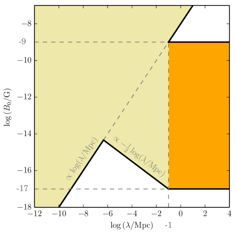
Figure 1: Constraints on $B_{0}$, the magnetic field strength today, as a function of the comoving scale $\lambda$. White regions are observationally excluded. Values above the diagonal line $\propto\log(\lambda/\mathrm{Mpc})$ have been processed by MHD and cannot be simply related to the primordial values. Orange marks the region that we use for constraints.

Observational constraints on the amplitude of magnetic fields on large scales today are summarised in LABEL:Durrer:2013pga. Combining theoretical bounds from magnetohydrodynamical turbulence decay, observational limits from Faraday rotation measurement, cosmic microwave background (CMB) anisotropies and spectral distortions, gamma ray observations, ultra-high-energy cosmic ray observations and constraints from initial seed fields for galactic dynamo, they get the following constraints for the current magnetic field strength $B_{0}$ in units of gauss (G) as a function of scale $\lambda$:

$$\log\bigg{(}\frac{B_{0}}{\mathrm{G}}\bigg{)}\in\begin{cases}\left[-17,-9\right]&\text{if }\log\left(\frac{\lambda}{\mathrm{Mpc}}\right)\in\left[-1,4\right]\vspace{0.1cm}\\ \left[-17.5-\frac{1}{2}\log\left(\frac{\lambda}{\mathrm{Mpc}}\right),-8+\log\left(\frac{\lambda}{\mathrm{Mpc}}\right)\right]&\text{if }\log\left(\frac{\lambda}{\mathrm{Mpc}}\right)\in\left[-6.3,-1\right]\vspace{0.1cm}\\ \left[-8+\log\left(\frac{\lambda}{\mathrm{Mpc}}\right),\text{no upper limit}\right]&\text{if }\log\left(\frac{\lambda}{\mathrm{Mpc}}\right)\in[-9,-6.3]\end{cases}\ .$$ (3.7)

These constraints on the observed power spectrum are shown in figure 1. The observational upper limit $B_{0}\lesssim 10^{-9}$ G comes mainly from the CMB and the Faraday rotation of radio emission spectra of distant quasars. The most important constraint is that on comoving wavelengths $\lambda>0.1$ Mpc, the amplitude has to be between $10^{-17}$ G and $10^{-9}$ G today. The lower limit comes from the non-observation of inverse Compton scattering from very high energy gamma rays and has the caveat that this could possibly be explained by plasma instabilities instead of large-scale coherent magnetic fields [1]. We follow the common interpretation of the observations in terms of a magnetic field. The Planck collaboration has reported the constraint $B_{0}<4.4$ nG at $\lambda=$ 1 Mpc [20]. They also get the marginalised constraint $n_{B}<-0.008$, but this has to be interpreted with care, as the constraint for a fixed amplitude can be quite different. The smaller the amplitude, the more freedom there is for the spectral index. Because the Planck data only gives an upper bound on $B_{0}$, it is consistent with any value of the spectral index for a small enough amplitude. The tilt $n_{B}$ of a power-law solution corresponds to the slope in figure 1 and the allowed values between 0.1 and $10^{4}$ Mpc translate to the upper and lower limits $|n_{B}+3|<3.2$, i.e. $-6.2<n_{B}<0.2$.

On small scales, the evolution is affected by the non-linear coupling between magnetic fields and plasma in the early universe. The system enters a turbulent regime, where energy is transferred from large to small scales and is eventually dissipated into heating up the plasma [1]. The line ${\rm log}(B_{0}/\mathrm{G})\propto{\rm log}(\lambda/$Mpc) in figure 1 corresponds to the largest possible regions that can have been processed by causal magnetohydrodynamics. Magnetic fields initially above the line (when scaled as $B_{0}=B_{\rm in}a_{\rm in}^{2},\lambda=\lambda_{\rm in}/a_{\rm in}$, where “$\rm{in}$” refers to the initial value; recall that $a_{0}=1$) decay through turbulence until they hit the line. Therefore there are no reliable constraints on the amplitude of primordial magnetic fields above the line. Although there is a lower limit on the observed magnetic fields between and $10^{-9}$ and $0.1$ Mpc that is below the magnetohydrodynamical line, it is not clear whether the origin of these fields is primordial, and, if so, whether their amplitude is simply scaled by $1/a^{2}$. We therefore exclude them from the analysis, and only consider the wavelengths between $\lambda_{2}=0.1$ Mpc and $\lambda_{1}=10^{4}$ Mpc. Including the smaller-scale modes would significantly tighten our constraints. On scales between $0.1$ Mpc and $10^{4}$ Mpc, the observational constraints on the amplitudes are below the magnetohydrodynamic line, so we assume that the magnetic fields retain their primordial spectrum and are only diluted by the expansion of the universe as $B\propto a^{-2}$. The magnetic power spectrum today is then simply related to the value at the end of inflation as $\delta_{B}(\eta_{0},k)=a_{\mathrm{end}}^{2}\delta_{B}(\eta_{\mathrm{end}},k)$.

Observational limits and the theoretical power spectrum.

Let us first consider the case $\alpha+\frac{1}{2}>0$. From Eq. (3.5) we have

$$\delta_{B}(\eta_{0},k) = a_{\mathrm{end}}^{2}\delta_{B}(\eta_{\mathrm{end}},k)$$ (3.8)

$$= \frac{\sqrt{(\alpha+1)^{2}+\sigma_{k}^{-2}}}{2\pi(2\alpha+1)}D^{-1}\left(\frac{k}{k_{\mathrm{end}}}\right)^{-\alpha+2}k_{\mathrm{end}}^{2}=\frac{\sqrt{(\alpha+1)^{2}+\sigma_{k}^{-2}}}{2\pi(2\alpha+1)}f(-k^{-1})^{-1}k^{2}$$

$$< 7.0\times 10^{-57}\sqrt{(\alpha+1)^{2}+\sigma_{k}^{-2}}f_{\mathrm{min}}^{-1}(\lambda/\mathrm{Mpc})^{-2}\ \mathrm{G}\,,$$

where we have put in $k=2\pi/\lambda$ and written $\lambda^{-2}=2.0\times 10^{-57}(\lambda/$Mpc$)^{-2}$ G. We have also taken into account that for $\delta_{B}\propto k^{-\alpha+2}$ the constraint $|n_{B}+3|<3.2$ implies $0.4<\alpha<3.6$. For the maximum comoving wavelength on which we have observational constraints, $\lambda_{1}=10^{4}$ Mpc, and the extreme value $f_{\mathrm{min}}^{-1}=10$, we get $\delta_{B}(\eta_{0},k_{1})<7\times 10^{-64}\sqrt{(\alpha+1)^{2}+\sigma_{k}^{-2}}$ G, many orders of magnitude below $10^{-17}$ G for any reasonable value of $\sigma_{k}$. The case $\alpha+\frac{1}{2}>0$ is therefore excluded.

Let us now look at the case $\alpha+\frac{1}{2}<0$. As $\delta_{B}\propto k^{\alpha+3}$, the constraint $|n_{B}+3|<3.2$ gives $-4.6<\alpha<-1.4$. We get the maximum amplitude when the second term in the square brackets in Eq. (3.6) is much larger than 1, in which case

$$\delta_{B}(\eta_{0},k) = a_{\mathrm{end}}^{2}\delta_{B}(\eta_{\mathrm{end}},k)=\frac{\sqrt{\alpha^{2}+\sigma_{k}^{-2}}}{2\pi}\kappa f(\eta_{2})\left(\frac{k}{k_{2}}\right)^{\alpha+3}k_{2}^{2}\ .$$ (3.9)

The amplitude is enhanced by the factor $f(\eta_{2})$. At $k_{2}=2\pi/(0.1$ Mpc) we have $\delta_{B}(\eta_{0},k_{2})<10^{-54}\sqrt{\alpha^{2}+\sigma_{k}^{-2}}\kappa f(\eta_{2})$ G, so we need $\sqrt{\alpha^{2}+\sigma_{k}^{-2}}\kappa f(\eta_{2})\geq 10^{37}$ to reach $10^{-17}$ G (as $\alpha<0$, $f(\eta_{2})>1$ guarantees that there is no strong coupling anywhere in the region of interest). However, $f(\eta_{2})$ cannot be increased without limit, as the electromagnetic energy density must not become so large as to spoil the success of inflation.

3.2 Backreaction and perturbations

Background constraint from backreaction.

We have to check that the contribution of the electromagnetic field to the energy density, Eqs. (2.13) and (2.1), disturbs neither the background evolution during inflation nor the generation of the curvature perturbation. Let us first consider the background contribution. A conservative limit is that the electromagnetic contribution to the energy density is less than the total energy density during inflation, $\rho_{BE}\equiv\rho_{B}+\rho_{E}<3M_{{}_{\mathrm{Pl}}}^{2}H^{2}$. Note that if the averaged equation of state during reheating is larger than $1/3$, the electromagnetic energy density could overtake the inflaton decay products and dominate the radiation density, in contradiction with observations. We do not consider the constraints arising from avoiding that.

The energy density of the electromagnetic field is given by an integral over the modes generated from the beginning of inflation. From Eqs. (2.1), (2.16), (2.19) and (2.2) we get for the electric contribution

$$\rho_{E}(\eta) > \frac{1}{a(\eta)^{4}f^{2}(\eta)}\frac{1}{2\pi^{2}}\int_{k_{\mathrm{beg}}}^{-\sigma_{k}^{-1}\eta^{-1}}\frac{\mathrm{d}k}{k}k^{3}|C_{2}(k)|^{2}$$ (3.10)

$$> \frac{1}{a(\eta)^{4}f^{2}(\eta)}\frac{1}{4\pi^{2}}\int_{k_{1}}^{-\sigma_{k}^{-1}\eta^{-1}}\mathrm{d}kk\left[f^{\prime}(-\sigma_{k}^{-1}k^{-1})^{2}+k^{2}f(-\sigma_{k}^{-1}k^{-1})^{2}\right]\,,$$

where we have dropped the contribution from the era before the observable modes are generated, since we know nothing about it. We know the form of $f$ between $k_{1}$ and $k_{2}$, but between $k_{2}$ and $k_{\mathrm{end}}$ we know only the initial and final values $f(\eta_{2})$ and $f(\eta_{\mathrm{end}})=1$, and that $f\geq f_{\mathrm{min}}$. We therefore get constraints during the time that the observable modes are generated and at the end of inflation, but not between.

During the time that the observational modes are generated, $\eta_{1}\leq\eta\leq\eta_{2}$, we obtain the following lower bound for the electric energy density

$$\rho_{E}(\eta) > \frac{\alpha^{2}+\sigma_{k}^{-2}}{8\pi^{2}(\alpha+2)}\sigma_{k}^{-2}\left[1-\left(-\eta\sigma_{k}k_{1}\right)^{2\alpha+4}\right]H^{4}\ .$$ (3.11)

This gives a non-trivial constraint when $\alpha+2<0$. For the magnetic energy density, we get similarly from Eqs. (2.13), (2.15), (2.19) and (2.2)

$$\rho_{B}(\eta) > \frac{\alpha^{2}+\sigma_{k}^{-2}}{8\pi^{2}(2\alpha+1)^{2}(\alpha+3)}\sigma_{k}^{-4}\left[1-\left(-\eta\sigma_{k}k_{1}\right)^{2\alpha+6}\right]H^{4}\,,$$ (3.12)

where we have dropped terms that are too small to be relevant. The magnetic field contribution is subdominant to the electric field contribution, except possibly for $\alpha\gtrsim-2$, in which case the constraint $\rho_{BE}<3M_{{}_{\mathrm{Pl}}}^{2}H^{2}$ is anyway trivially satisfied. The background constraints are strongest at $\eta_{2}$. Requiring $\rho_{E}<3M_{{}_{\mathrm{Pl}}}^{2}H^{2}$ with Eq. (3.11) gives the constraint $\alpha>-3.0$, using $H/M_{{}_{\mathrm{Pl}}}<3\times 10^{-5}$. This value is for $\sigma_{k}=1$, but the dependence on $\sigma_{k}$ is only logarithmic.

At the end of inflation we have for the electric field

$$\rho_{E}(\eta_{\mathrm{end}}) > \frac{1}{a_{\mathrm{end}}^{4}}\frac{1}{4\pi^{2}}\int_{k_{1}}^{k_{\mathrm{end}}}\mathrm{d}kk\left[f^{\prime}(-\sigma_{k}^{-1}k^{-1})^{2}+k^{2}f(-\sigma_{k}^{-1}k^{-1})^{2}\right]$$ (3.13)

$$= \frac{1}{a_{\mathrm{end}}^{4}}\frac{1}{4\pi^{2}}\left\{\int_{k_{1}}^{k_{2}}\mathrm{d}kk\left[f^{\prime}(-\sigma_{k}^{-1}k^{-1})^{2}+k^{2}f(-\sigma_{k}^{-1}k^{-1})^{2}\right]\right.$$

$$\left.+\int_{k_{2}}^{k_{\mathrm{end}}}\mathrm{d}kk\left[f^{\prime}(-\sigma_{k}^{-1}k^{-1})^{2}+k^{2}f(-\sigma_{k}^{-1}k^{-1})^{2}\right]\right\}$$

$$> \frac{1}{a_{\mathrm{end}}^{4}}\frac{1}{4\pi^{2}}\left\{\int_{k_{1}}^{k_{2}}\mathrm{d}kk\left[f^{\prime}(-\sigma_{k}^{-1}k^{-1})^{2}+k^{2}f(-\sigma_{k}^{-1}k^{-1})^{2}\right]\right.$$

$$\left.+\int_{k_{2}}^{k_{\mathrm{end}}}\mathrm{d}kkf^{\prime}(-\sigma_{k}^{-1}k^{-1})^{2}\right\}\ .$$

In the integral from $k_{1}$ to $k_{2}$, we can insert the known form of $f$. We can write the integral from $k_{2}$ to $k_{\mathrm{end}}$ as $\int_{k_{2}}^{k_{\mathrm{end}}}\mathrm{d}kkf^{\prime}(-\sigma_{k}^{-1}k^{-1})^{2}=4\sigma_{k}^{-2}\int_{x_{\mathrm{end}}}^{x_{2}}\mathrm{d}x(\mathrm{d}f/\mathrm{d}x)^{2}\geq 4\sigma_{k}^{-2}[f(\eta_{2})-1]^{2}/(x_{2}-x_{\mathrm{end}})$, where $x=(\sigma_{k}k)^{-4}$. The inequality follows from writing the integral as an average over the range from $x_{\mathrm{end}}$ to $x_{2}$ and using the fact that variance is non-negative: $\int_{x_{\mathrm{end}}}^{x_{2}}\mathrm{d}x(\mathrm{d}f/\mathrm{d}x)^{2}\equiv(x_{2}-x_{\mathrm{end}})\langle{(\mathrm{d}f/\mathrm{d}x)^{2}}\rangle\geq(x_{2}-x_{\mathrm{end}})\langle{\mathrm{d}f/\mathrm{d}x}\rangle^{2}$. The result is, dropping terms that are too small to be relevant,

$$\rho_{E}(\eta_{\mathrm{end}}) > \frac{\sigma_{k}^{-2}}{\pi^{2}}f^{2}(\eta_{2})\left(\frac{k_{2}}{k_{\mathrm{end}}}\right)^{4}\left\{\frac{\alpha^{2}+\sigma_{k}^{-2}}{8(\alpha+2)}\left[1-\left(\frac{k_{1}}{k_{2}}\right)^{2\alpha+4}\right]+1\right\}H^{4}\ .$$ (3.14)

For the magnetic field energy density we get

$$\rho_{B}(\eta_{\mathrm{end}}) > \frac{\alpha^{2}+\sigma_{k}^{-2}}{8\pi^{2}(\alpha+3)}\sigma_{k}^{-4}\kappa^{2}f^{2}(\eta_{2})\left(\frac{k_{2}}{k_{\mathrm{end}}}\right)^{4}\left[1-\left(\frac{k_{1}}{k_{2}}\right)^{2\alpha+6}\right]H^{4}\ .$$ (3.15)

For $\alpha\gtrsim-2$, the constraint from the magnetic field can be more stringent than the one from the electric field.

Making use of Eq. (3.9) to replace $f(\eta_{2})$, the limit $\rho_{E}(\eta_{\mathrm{end}})+\rho_{B}(\eta_{\mathrm{end}})<3M_{{}_{\mathrm{Pl}}}^{2}H^{2}$ can be evaluated with Eqs. (3.14) and (3.15) and we obtain

$$\delta_{B}(\eta_{0},k) < 4\sqrt{3}\pi^{2}\frac{M_{{}_{\mathrm{Pl}}}}{H}\kappa\left\{\frac{\sigma_{k}^{2}}{2\alpha+4}\left[1-\left(\frac{k_{1}}{k_{2}}\right)^{2\alpha+4}\right]+\frac{\kappa^{2}}{2\alpha+6}\left[1-\left(\frac{k_{1}}{k_{2}}\right)^{2\alpha+6}\right]\right.$$ (3.16)

$$\left.+\frac{4\sigma_{k}^{2}}{\alpha^{2}+\sigma_{k}^{-2}}\right\}^{-\frac{1}{2}}\left(\frac{k}{k_{2}}\right)^{\alpha+3}(\sigma_{k}^{-1}\lambda_{\mathrm{end}})^{-2}$$

$$\approx 4.6\times 10^{-51}\kappa\left(\frac{r}{0.07}\right)^{-\frac{1}{2}}\left\{\frac{\sigma_{k}^{2}}{2\alpha+4}\left[1-\left(\frac{k_{1}}{k_{2}}\right)^{2\alpha+4}\right]+\frac{\kappa^{2}}{2\alpha+6}\left[1-\left(\frac{k_{1}}{k_{2}}\right)^{2\alpha+6}\right]\right.$$

$$\left.+\frac{4\sigma_{k}^{2}}{\alpha^{2}+\sigma_{k}^{-2}}\right\}^{-\frac{1}{2}}\left(\frac{k}{k_{2}}\right)^{\alpha+3}\left(\frac{\sigma_{k}^{-1}\lambda_{\mathrm{end}}}{\mathrm{Mpc}}\right)^{-2}G\ .$$

The quantity $\sigma_{k}^{-1}\lambda_{\mathrm{end}}$ is the smallest wavelength that exits the Hubble radius during inflation. It depends on the inflationary scale and the dynamics of preheating,

$$\sigma_{k}^{-1}\lambda_{\mathrm{end}} = \frac{2\pi}{a_{\mathrm{end}}H}=\frac{2\pi\sqrt{3}M_{{}_{\mathrm{Pl}}}}{a_{\mathrm{end}}\sqrt{\rho_{\mathrm{end}}}}$$ (3.17)

$$= 2\pi\sqrt{3}M_{{}_{\mathrm{Pl}}}\left[\frac{g_{*}(T_{\mathrm{reh}})}{g_{*}(T_{0})}\right]^{\frac{1}{12}}\left(\rho_{\mathrm{reh}}\rho_{\gamma 0}\right)^{-\frac{1}{4}}\left(\frac{\rho_{\mathrm{reh}}}{\rho_{\mathrm{end}}}\right)^{\frac{1+3\bar{w}}{6(1+\bar{w})}}$$

$$\approx 140\times 10^{-6}\left[\frac{g_{*}(T_{\mathrm{reh}})}{10.75}\right]^{\frac{1}{12}}\left(\frac{\rho_{\mathrm{reh}}}{\rho_{\mathrm{BBN}}}\right)^{-\frac{1}{4}}\left(\frac{\rho_{\mathrm{reh}}}{\rho_{\mathrm{end}}}\right)^{\frac{1+3\bar{w}}{6(1+\bar{w})}}\mathrm{Mpc}$$

$$> 140\times 10^{-6}\left(\frac{\rho_{\mathrm{end}}}{\rho_{\mathrm{BBN}}}\right)^{-\frac{1}{4}}\mathrm{Mpc}\approx 5.2\times 10^{-23}\left(\frac{r}{0.07}\right)^{-\frac{1}{4}}\mathrm{Mpc}\,,$$

where we have used the adiabatic relation $g_{*S}(T)T^{3}a^{3}=$ constant, “${\mathrm{reh}}$” refers to reheating, $\rho_{\gamma 0}=\frac{\pi^{2}}{15}T_{0}^{4}$ with $T_{0}=2.725$ K is the radiation energy density today, $-1/3<\bar{w}<1$ is the average (over the number of e-folds) equation of state between the end of inflation and the onset of the radiation era, and $g_{*}$ is the effective number of energy degrees of freedom, which we have assumed to be the same as the effective number of entropy degrees of freedom $g_{*S}$. On the next-to-last line we have inserted the lower limit on the reheating energy density from big bang nucleosynthesis, which is $\rho_{\mathrm{BBN}}=\frac{\pi^{2}}{30}g_{*}(T_{\mathrm{BBN}})T_{\mathrm{BBN}}^{4}$ where $T_{\mathrm{BBN}}=4.7$ MeV is the lowest possible temperature for thermalisation of Standard Model particles after inflation [35]; as $g_{*}(4.7\ \mathrm{MeV})=10.75$, this gives $\rho_{\mathrm{reh}}^{1/4}>\rho_{\mathrm{BBN}}^{1/4}=6.4$ MeV. On the last line we have written $H/M_{{}_{\mathrm{Pl}}}=3\times 10^{-5}(r/0.07)^{\frac{1}{2}}$, see footnote 2, corresponding to $\rho_{\mathrm{end}}^{1/4}=3\times 10^{16}(r/0.07)^{\frac{1}{4}}$ GeV. Note that we can get the lower limit in two different ways. If $\bar{w}\leq 1/3$, we maximise $\rho_{\mathrm{reh}}$ by putting it equal to $\rho_{\mathrm{end}}$, in which case $\bar{w}$ is irrelevant. If $\bar{w}\geq 1/3$, we minimise $\rho_{\mathrm{reh}}$ by putting it equal to $\rho_{\mathrm{BBN}}$, in which case $\bar{w}=1/3$ gives the minimal amplitude. In both cases the density factors reduce to $(\rho_{\mathrm{end}}/\rho_{\mathrm{BBN}})^{-1/4}$.

Inserting Eq. (3.17) into Eq. (3.16), we have

$$\delta_{B}(\eta_{0},k) < 1.7\times 10^{-6}\kappa\left\{\frac{\sigma_{k}^{2}}{2\alpha+4}\left[1-\left(\frac{k_{1}}{k_{2}}\right)^{2\alpha+4}\right]+\frac{\kappa^{2}}{2\alpha+6}\left[1-\left(\frac{k_{1}}{k_{2}}\right)^{2\alpha+6}\right]\right.$$ (3.18)

$$\left.+\frac{4\sigma_{k}^{2}}{\alpha^{2}+\sigma_{k}^{-2}}\right\}^{-\frac{1}{2}}\left(\frac{k}{k_{2}}\right)^{\alpha+3}\mathrm{G}\ .$$

Note that the dependence on $r$ (i.e. on the inflationary energy scale) drops out. In the case where the second term (i.e. the magnetic contribution) or the last term dominates, the constraint is anyway too weak to be relevant, so only the first term is important. Taking into account $\alpha\geq-3.0$, the most difficult amplitude to reproduce is the one on the largest wavelengths. We get the following $\alpha$-dependent constraint on the amplitude:

$$\delta_{B}(\eta_{0},k_{1}) < 1.7\times 10^{-6}\sigma_{k}^{-1}\kappa\left\{\frac{1}{2\alpha+4}\left[1-\left(\frac{k_{1}}{k_{2}}\right)^{2\alpha+4}\right]\right\}^{-\frac{1}{2}}\left(\frac{k_{1}}{k_{2}}\right)^{\alpha+3}\mathrm{G}\ .$$ (3.19)

The maximum value is reached for $\alpha=-3$,

$$\delta_{B}(\eta_{0},k_{1}) < 2\times 10^{-11}\sigma_{k}^{-1}\kappa\mathrm{G}\,,$$ (3.20)

and we get the minimal value for $\alpha=-1.4$,

$$\delta_{B}(\eta_{0},k_{1}) < 2\times 10^{-14}\sigma_{k}^{-1}\kappa\mathrm{G}\ .$$ (3.21)

While in principle we could get a magnetic field amplitude of $10^{-9}$ G by taking $\kappa=100$, this would correspond to an extremely fine-tuned situation. The function $f$ (and thus the QED coupling) would have to jump immediately at the end of the observational window to the value $f_{\mathrm{min}}$ at the limit of perturbativity, and then to the standard value $f=1$ immediately before the end of inflation. Also, in this case the contribution from $f^{\prime 2}$ between $k_{2}$ and $k_{\mathrm{end}}$ (which we have neglected) would be large, and we would have to jointly minimise the contribution from $\kappa$ (which calls for a rapid shift in $f$) and the constraint from $f^{\prime 2}$ (which calls for $f$ not to change rapidly). We do not consider such optimisation, but now consider the limit from perturbations, which turns out to be stronger than the background limit.

Constraint from perturbations.

We consider the gauge invariant curvature perturbation $\zeta=-\psi-H\delta\rho/\dot{\rho}$, which receives contributions both from the inflaton and the electromagnetic field. Assuming single-field slow-roll inflation, the spectrum of the inflaton contribution $\zeta_{I}$ is

$$\mathcal{P}_{\zeta_{I}} = \frac{1}{8\pi^{2}\epsilon}\frac{H^{2}}{M_{{}_{\mathrm{Pl}}}^{2}}\,,$$ (3.22)

where $\epsilon$ is the first slow-roll parameter. The contribution of the electromagnetic energy density to the curvature perturbation is

$$\zeta_{BE} = -H\frac{\delta\rho_{BE}}{\dot{\rho}}=\frac{\delta\rho_{BE}}{6\epsilon M_{{}_{\mathrm{Pl}}}^{2}H^{2}}=\frac{4\pi^{2}}{3}\mathcal{P}_{\zeta_{I}}\frac{\delta\rho_{BE}}{H^{4}}\,,$$ (3.23)

where we have inserted $\dot{\rho}=-6\epsilon M_{{}_{\mathrm{Pl}}}^{2}H^{3}$ and used Eq. (3.22).

The component $\zeta_{BE}$ is non-Gaussian since $\rho_{BE}$ given in Eq. (2.1) is quadratic in the vector potential ${\cal A}$. The electromagnetic field is therefore constrained both by the observed amplitude of the total curvature perturbation ${\cal P}_{\zeta}=2.2\times 10^{-9}$ [36] and by observational bounds on primordial non-Gaussianity. Detailed investigation of the non-Gaussian signatures [21, 22, 23, 24, 25, 26, 27, 28, 19] is beyond the scope of our current work. To get a rough constraint, we approximate the magnitude of the bispectrum as $\langle\zeta^{3}\rangle\sim{\cal P}_{\zeta_{BE}}^{\frac{3}{2}}$ and use the Planck limit on local non-Gaussianity $f_{\rm NL}=2.5\pm 5.7$ [37]. This constrains the contribution of ${\cal P}_{\zeta_{BE}}$ to the total spectrum to be at most at the percent level. Moreover, if the magnetic contribution ${\cal P}_{\zeta_{BE}}$ is strongly scale dependent, the measured scale invariance of primordial perturbations yields a quantitatively similar constraint. To account for both constraints, we parameterise the electromagnetic contribution to the power spectrum as $\mathcal{P}_{\zeta_{BE}}\leq 10^{-2}\mathcal{P}_{\zeta}\sigma_{\zeta}$, with the default value $\sigma_{\zeta}=1$. If $\mathcal{P}_{\zeta_{BE}}$ is close to scale invariant, its contribution could possibly be larger, given that the electromagnetic and matter perturbations could equilibrate in reheating, so that there are no isocurvature perturbations observable in the CMB. The parameter $\sigma_{\zeta}$ can be adjusted to suit, and our limits anyway turn out not to depend strongly on $\sigma_{\zeta}$.

As the electromagnetic field is assumed to be energetically subdominant during inflation, its fluctuations generate isocurvature perturbations. Therefore the total curvature perturbation $\zeta=\zeta_{I}+\zeta_{BE}$ is not conserved but evolves during and after inflation. The evolution of $\zeta$ depends on the details of reheating, see e.g. LABEL:Bonvin:2011dt. After reheating the universe contains a large number of charged particles that rapidly dissipate the electric field. Because the magnetic fields scale as radiation $B^{2}\propto a^{-4}$ on superhorizon scales, the magnetic contribution to the curvature perturbation (3.23) remains constant during radiation domination. A detailed analysis of the evolution is beyond the scope of our current work, and we look only at the electromagnetic contribution to the curvature perturbation at the end of inflation, $\zeta_{BE}(\eta_{\rm end})$. If its contribution to the total power spectrum is small compared to the observed amplitude, the electromagnetic contribution to the final curvature perturbation is expected to be small.

Using the expression (2.1) of the electromagnetic energy density, we can express the spectrum of $\zeta_{BE}$ at the end of inflation as

$${\cal P}_{\zeta_{BE}}^{\rm end} = \left(\mathcal{P}^{\rm end}_{\zeta_{I}}\right)^{2}\;\frac{(2\pi)^{5}k^{3}}{9H^{8}}\int\mathrm{d}^{3}q\left\{\left[P_{E}(q)P_{E}(|{\bf k-q}|)+P_{B}(q)P_{B}(|{\bf k-q}|)\right]\right.$$ (3.24)

$$\times\left.\left(1+{\rm cos}^{2}\theta\right)-4{\rm cos}\theta\;{\rm Re}\left[P_{BE}(q)P_{BE}(|{\bf k-q}|)\right]\right\}$$

$$\gtrsim \left(\mathcal{P}^{\rm end}_{\zeta_{I}}\right)^{2}\;\frac{(2\pi)^{5}k^{3}}{9H^{8}}\int_{k_{1}<q,|{\bf k}-{\bf q}|<k_{2}}\mathrm{d}^{3}q\left\{\left[P_{E}(q)P_{E}(|{\bf k-q}|)+P_{B}(q)P_{B}(|{\bf k-q}|)\right]\right.$$

$$\times\left.\left(1+{\rm cos}^{2}\theta\right)-4{\rm cos}\theta\;{\rm Re}\left[P_{BE}(q)P_{BE}(|{\bf k-q}|)\right]\right\}\,,$$

where $\theta$ is the angle between ${\bf q}$ and ${\bf k-q}$. The magnetic and electric power spectra used here are related to Eqs. (2.15) and (2.16) as $P_{B}\equiv\delta_{B}^{2}/(4\pi k^{3}f^{2})$ and $P_{E}\equiv\delta_{E}^{2}/(4\pi k^{3}f^{2})$. The cross spectrum is defined as $\langle B_{i}{}^{*}({\bf k})E_{j}{}({\bf k^{\prime}})\rangle=-(2\pi)^{3}\delta({\bf k}-{\bf k^{\prime}})i\epsilon_{ijk}\hat{k}^{k}P_{BE}(k)$, with $P_{BE}\equiv k({\cal A}/f)({\cal A}/f)^{\prime}{}^{*}/[a^{4}(2\pi)^{3}]$. On the second line we have taken into account that while we cannot evaluate the convolution integrals in Eq. (3.24) without knowing the full form of the coupling $f(\eta)$, we can get a lower limit for the full result by calculating the result in the range $k_{1}<k<k_{2}$. As the third term in the integrand is not positive definite, this limit is not watertight. However, as the electric contribution usually dominates over the magnetic contribution and the electric-magnetic cross term is oscillatory, we expect that our lower limit is valid, barring fine-tuned cases. We use the power-law form $f=D(k_{\rm end}/k)^{-\alpha}$ in the window $k_{1}<k<k_{2}$ and substitute the asymptotic solution (3.1), which leaves us with convolutions of the form $\int\mathrm{d}^{3}qq^{n}|{\bf k}-{\bf q}|^{n}$. We use methods similar to the ones presented in Refs. [39, 40, 41] and estimate the integrals by including contributions from the three regimes, $q\ll k$, $q\sim k$ and $q\gg k$. This gives a reasonable order of magnitude estimate, which suffices for our purposes.

$$\frac{\mathcal{P}_{\zeta_{BE}}^{\rm end}}{(\mathcal{P}^{\rm end}_{\zeta_{I}})^{2}} \gtrsim \frac{f(\eta_{2})^{4}(\alpha^{2}+\sigma_{k}^{-2})^{2}}{18}\sigma_{k}^{-4}\left(\frac{k_{2}}{k_{\rm end}}\right)^{8}\left(\frac{k}{k_{2}}\right)^{3}\Bigg{\{}\kappa^{4}\sigma_{k}^{-4}I_{2\alpha+3}(k)+I_{2\alpha+1}(k)$$ (3.25)

$$\left.+\frac{4\kappa^{2}\sigma_{k}^{-2}}{4\alpha+7}\left[1-\left(\frac{k}{k_{2}}\right)^{4\alpha+7}\right]\right\}$$

$$= \frac{\delta^{4}_{B}(\eta_{0},k)(\sigma_{k}^{-1}\lambda_{\mathrm{end}})^{8}}{18(2\pi)^{4}}\left(\frac{k}{k_{2}}\right)^{-4\alpha-9}\Bigg{\{}I_{2\alpha+3}(k)+\kappa^{-4}\sigma_{k}^{4}I_{2\alpha+1}(k)$$

$$\left.+\frac{4\kappa^{-2}\sigma_{k}^{2}}{4\alpha+7}\left[1-\left(\frac{k}{k_{2}}\right)^{4\alpha+7}\right]\right\}\,,$$

where

$$I_{n}(k)\equiv\frac{1}{2n+3}\left[1-\left(\frac{k}{k_{2}}\right)^{2n+3}\right]+\frac{2}{n+3}\left(\frac{k}{k_{2}}\right)^{n}\left[\left(\frac{k}{k_{2}}\right)^{n+3}-\left(\frac{k_{1}}{k_{2}}\right)^{n+3}\right]\,,$$ (3.26)

and on the second line of Eq. (3.25) we have used Eq. (3.9).

The condition $\mathcal{P}_{\zeta_{BE}}^{\rm end}\leq 10^{-2}\sigma_{\zeta}\mathcal{P}_{\zeta}^{\rm end}$ ensuring that the spectrum of $\zeta_{BE}$ at the end of inflation is smaller than the observed spectrum of curvature perturbations then translates Eq. (3.25) into an upper bound on $\delta_{B}(\eta_{0},k)$. Violation of this condition does not strictly rule out the setup, because the curvature perturbation evolves over reheating and this might decrease $\zeta$ to the observed level. However, we may at least argue that CMB observations imply quite non-trivial constraints for such scenarios.

Given $-3.0<\alpha<-1.4$, the middle term in Eq. (3.25) (which arises from the purely electric contribution) gives the strongest bound, which comes from the longest wavelength. Using $\mathcal{P}_{\zeta_{BE}}^{\rm end}\leq 10^{-2}\sigma_{\zeta}\mathcal{P}_{\zeta}^{\rm end}$, assuming that the electromagnetic contribution is clearly subdominant, $\mathcal{P}_{\zeta_{I}}\approx\mathcal{P}_{\zeta}=2.2\times 10^{-9}$, and using the lower limit (3.17) on $\sigma_{k}^{-1}\lambda_{\mathrm{end}}$, the constraint from Eq. (3.25) is

$$\delta_{B}(\eta_{0},k_{1})<5\times 10^{-15}|4\alpha+5|^{1/4}\left(\frac{r}{0.07}\right)^{\frac{1}{2}}\sigma_{k}^{-1}\sigma_{\zeta}^{1/4}\kappa\mathrm{G}\ .$$ (3.27)

The dependence on $\alpha$ is weak, since $|4\alpha+5|^{1/4}\simeq 0.9$ for $\alpha=-1.4$ and $\simeq 1.6$ for $\alpha=-3$.

Note that the perturbation constraint (3.27) depends crucially on the assumption that the observed curvature perturbation is dominantly generated by the inflaton. It does not apply if the inflaton contribution to the total curvature perturbation is small, as in the curvaton scenario [42, 43, 44]. The electromagnetic energy density goes down as $a^{-4}$ after reheating, the same way as the inflaton decay products, so the curvaton will dampen its contribution to the total perturbation in the same way as it dampens the inflaton contribution. Hence the perturbative constraint disappears in this case.

4 Conclusions

Comparison to previous work.

A number of earlier papers have put constraints of varying degrees of generality on magnetogenesis models where the conformal symmetry is broken by $f(\phi)$, starting from LABEL:Demozzi:2009fu, which noted that a power-law form leads to either the backreaction or strong coupling problem, or to a too small amplitude. In LABEL:Ferreira:2013sqa the authors consider a form of $f(\phi)$ tuned to avoid these problems, as well as the effect of optimising the reheating history (and assuming the curvaton scenario to decouple the amplitude of inflationary perturbations and the Hubble scale), with a maximum amplitude of $10^{-17}$ G around $10^{4}$ Mpc today and $10^{-13}$ G on Mpc scales. They consider the strong coupling problem and backreaction problem, but not the effect of the electromagnetic perturbations, which gives our strongest limit. These values are consistent with our background-only limit, although this need not have been the case, as the spectrum of LABEL:Ferreira:2013sqa is not a power law. In LABEL:Ferreira:2014hma the authors consider a power-law form for $f$ and take into account the bispectrum (which we did not consider). They find a maximum value of $10^{-15}$ G on Mpc scales. Contrary to our case where $f$ can have arbitrary form between the end of the observational window and the end of inflation, both papers find the maximum amplitude for the lowest inflationary scale.

Some studies have derived upper limits by adopting a power-law description of quantities related directly to the magnetic field rather than to the coupling function and other more model-independent studies [14, 16, 18]. However, in this case it is not possible to consider the important strong coupling constraint. The study [6] is rather model-independent and takes the strong coupling issue into account, but it only gives an upper limit on the minimum value of the magnetic field, not on the maximum possible value.

It is easy to understand why our background constraint is independent of the inflationary scale. The maximum magnetic energy density is proportional to the total energy density during inflation. If the inflationary scale is higher, then on the one hand the magnetic field amplitude at the end of inflation is larger. On the other hand, the universe has to expand by a larger factor to end up at the radiation energy density today, fixed by the measured CMB temperature. For instantaneous reheating, the energy density in the inflaton decay products goes like $\propto a^{-4}$, like the magnetic energy density, so the two effects exactly compensate each other. Taking into account different reheating histories and the change in the number of relativistic degrees of freedom does not change the conclusion for the maximum magnetic field amplitude. For the perturbative constraints, the amplitude of the induced curvature perturbations is proportional to the magnetic energy density, but the total curvature perturbation, to which we compare, is fixed by observation, so the first above mentioned effect is absent, and we are left with the dependence $\delta_{B}(\eta_{0},k)\propto r^{1/2}$. If we used the theoretical inflaton spectrum (3.22) instead and assumed $\epsilon<1$ (as done in LABEL:Fujita:2014sna) or fixed $\epsilon=0.01$ (as done in LABEL:Ferreira:2014hma), our perturbative limit would have a less stringent dependence on $r$.

Summary.

We find that the requirement that the power spectrum today on the observed scales is a power law determines the coupling $f$ to essentially be a power law, $f\propto\eta^{-\alpha}$. Crucially, we make no assumptions about the form of $f$ outside the window where the observable modes are generated, apart from avoiding strong coupling. We take this range of scales to be between 0.1 Mpc and $10^{4}$ Mpc. From the constraint on the backreaction on the background evolution in the observable window and at the end of inflation, optimising over all possible reheating histories described by an average equation of state $-1/3<\bar{w}<1$, we find the limit

$$\delta_{B}(\eta_{0},k_{1}) < 2\times 10^{-14}\sigma_{k}^{-1}\kappa\,\mathrm{G}\,,$$ (4.1)

where $\sigma_{k}$ parametrises the uncertainty due to our approximation of matching the sub- and super-Hubble modes when solving for the magnetic field, and is not expected to be much different from unity. The parameter $\kappa$ parametrises the unknown form of $f$ outside the observational window, and is $<100$. This is a conservative bound, and it is not guaranteed that there exists a function $f$ that can saturate it. If such a function exists, it will be extremely fine-tuned, and we would naturally expect $\kappa\ll 1$. We also find that the spectral index of the magnetic field has to lie between $-3<n_{B}<0.2$, i.e. $-1.4<\alpha<-3$.

Taking into account that the electromagnetic perturbations cannot disturb the power spectrum of curvature perturbations too much, we get the limit

$$\delta_{B}(\eta_{0},k_{1})<5\times 10^{-15}|4\alpha+5|^{1/4}\left(\frac{r}{0.07}\right)^{1/2}\sigma_{k}^{-1}\sigma_{\zeta}^{1/4}\kappa\,\mathrm{G}\,,$$ (4.2)

where $\sigma_{\zeta}$ is the maximum fractional contribution of the electromagnetic power spectrum contribution to the total curvature power spectrum, with $\sigma_{\zeta}=1$ corresponding to a maximum of $10^{-2}$. This limit is more stringent, but it can be avoided if the curvature perturbation is not generated by the inflaton but for example via the curvaton mechanism. We only consider the perturbative limit at the end of inflation, but evolution during and after inflation could modify this bound.

The assumption of a power-law form for the observed magnetic field and the lever arm of five orders of magnitude in wavelength are important for our limits. If we extend the constraints down to lengths of $\lambda_{2}=10^{-6}$ Mpc, the requirement on the amplitude tightens linearly with $\lambda_{2}$, which makes the electromagnetic contribution to the curvature perturbations too large if the latter are generated through the standard inflationary mechanism. If we go all the way to $10^{-9}$ Mpc, the backreaction becomes too large at the level of the background already and the mechanism we discussed is ruled out altogether. Considering a more general spectrum could loosen the constraints, and more detailed investigation of the bispectrum and other higher-order statistics could lead to more stringent constraints.

Appendix A Form of the coupling function

From the magnetic power spectrum to the coupling function.

Here we show that if the magnetic spectrum is a power law, $\delta_{B}(\eta_{0},k)^{2}\propto k^{n_{B}+3}$ in the observable region $k_{1}\leq k\leq k_{2}$, then $f$ can significantly deviate from a power law only for a small range of e-folds. From Eqs. (2.2) and (3.1) we have

$$\delta_{B}(\eta_{\mathrm{end}},k)^{2} \propto k^{5}\left|C_{1}(k)+C_{2}(k)\int^{\eta_{\mathrm{end}}}_{\eta_{2}}\frac{\mathrm{d}\tau}{f(\tau)^{2}}\right|^{2}$$ (A.1)

$$\propto k^{4}\left.\left[g^{\prime}(\eta)^{2}+k^{2}g(\eta)^{2}\right]\right|_{\eta=-(\sigma_{k}k)^{-1}}\,,\quad$$

where we have denoted $g(\eta)\equiv-F(\eta)-\kappa(\eta_{2}-\eta_{\mathrm{end}})f(\eta)>0$. Writing $\dot{g}\equiv\mathrm{d}g/\mathrm{d}N=\eta_{\mathrm{end}}e^{N}g^{\prime}$ and $n\equiv\frac{1}{2}(n_{B}-3)$, we get

$$\mathrm{e}^{-2nN}\propto\dot{g}^{2}+\sigma_{k}^{-2}g^{2}\ .$$ (A.2)

Writing $g(N)=h(N)\mathrm{e}^{-nN}$, the solution of Eq. (A.2) is given by

$$h = h_{0}\sin[\phi(N)]$$ (A.3)

$$\dot{h}-nh = h_{0}\sigma_{k}^{-1}\cos[\phi(N)]\,,$$ (A.4)

where $h_{0}>0$ is a constant. The condition $g>0$ implies $0<\phi<\pi$. Eliminating $h$, we find that $\phi(N)$ satisfies the equation

$$\dot{\phi}=\sigma_{k}^{-1}+n\tan\phi\ .$$ (A.5)

Sum of two power-laws.

If $\dot{\phi}=0$, the constant $\phi\equiv\phi_{c}$ is given by $\sigma_{k}^{-1}+n\tan\phi_{c}=0$. Then $g$ is a power-law, $F+\kappa(\eta_{2}-\eta_{\mathrm{end}})f\propto e^{-nN}\propto\eta^{-n}$. This implies that

$$f(\eta)=D\left(\frac{\eta}{\eta_{2}}\right)^{-n}+\frac{1}{2}\left[\sqrt{D^{2}-\frac{4}{(2n+1)\kappa(1-\eta_{\mathrm{end}}/\eta_{2})}}-D\right]\left(\frac{\eta}{\eta_{2}}\right)^{n+1}\,,$$ (A.6)

where $D$ is a constant. Unless $D$ is zero or tuned to make the second term vanish, $f$ is not a power law. However, in order to get a large enough amplitude to match observations, $D$ must be very large (for the reasons discussed in section 3.1), so the second term is negligible, and $f$ is close to a power-law.

Deviations from power-law behaviour.

If $\dot{\phi}\neq 0$, the solution has two branches,

$$\sigma_{k}^{-1}(\sigma_{k}^{2}n^{2}+1)(N+N_{c}) = \phi+\sigma_{k}n\ln(\cos\phi+\sigma_{k}n\sin\phi)$$ (A.7)

$$\sigma_{k}^{-1}(\sigma_{k}^{2}n^{2}+1)(N+N_{c}) = \phi+\sigma_{k}n\ln(-\cos\phi-\sigma_{k}n\sin\phi)\,,$$ (A.8)

where $N_{c}$ is an integration constant. The first branch covers $0<\phi<\phi_{c}<\pi/2$ and the second covers $\phi_{c}<\phi<\pi$. If $\phi$ does not go near $0$ or $\pi$, the modification to the power-law amplitude due to $\sin\phi$ is less than unity, and occurs only for a limited range of e-folds, so $f$ is essentially a power law. If $\phi$ approaches $0$ or $\pi$, the amplitude of $f$ can be damped by an arbitrarily large factor at small or large $N$, respectively (note that, by construction, the observed power spectrum is unaffected, as the decrease in $f$ is compensated by an increase in $f^{\prime}$). However, this only changes $f$ in a small region that has to be tuned to be near either the end or the beginning of the observational window. Even in this fine-tuned case, $f$ deviates from a power law only for a small range of e-folds, and this does not change our results.

References

- [1] R. Durrer and A. Neronov, Cosmological Magnetic Fields: Their Generation, Evolution and Observation, Astron. Astrophys. Rev. 21 (2013) 62, [1303.7121].
- [2] R. Pakmor, F. Marinacci and V. Springel, Magnetic fields in cosmological simulations of disk galaxies, Astrophys. J. 783 (2014) L20, [1312.2620].
- [3] M. S. Turner and L. M. Widrow, Inflation Produced, Large Scale Magnetic Fields, Phys. Rev. D37 (1988) 2743.
- [4] B. Ratra, Cosmological ’seed’ magnetic field from inflation, Astrophys. J. 391 (1992) L1–L4.
- [5] V. Demozzi, V. Mukhanov and H. Rubinstein, Magnetic fields from inflation?, JCAP 0908 (2009) 025, [0907.1030].
- [6] T. Fujita and S. Mukohyama, Universal upper limit on inflation energy scale from cosmic magnetic field, JCAP 1210 (2012) 034, [1205.5031].
- [7] R. J. Z. Ferreira, R. K. Jain and M. S. Sloth, Inflationary magnetogenesis without the strong coupling problem, JCAP 1310 (2013) 004, [1305.7151].
- [8] S. Kanno, J. Soda and M.-a. Watanabe, Cosmological Magnetic Fields from Inflation and Backreaction, JCAP 0912 (2009) 009, [0908.3509].
- [9] S. Kanno, M. Kimura, J. Soda and S. Yokoyama, Anisotropic Inflation from Vector Impurity, JCAP 0808 (2008) 034, [0806.2422].
- [10] J. M. Wagstaff and K. Dimopoulos, Particle Production of Vector Fields: Scale Invariance is Attractive, Phys. Rev. D83 (2011) 023523, [1011.2517].
- [11] K. Dimopoulos, G. Lazarides and J. M. Wagstaff, Eliminating the -problem in SUGRA Hybrid Inflation with Vector Backreaction, JCAP 1202 (2012) 018, [1111.1929].
- [12] M. Karčiauskas, Dynamical Analysis of Anisotropic Inflation, Mod. Phys. Lett. A31 (2016) 1640002, [1604.00269].
- [13] M. Giovannini, Large-scale magnetic fields, curvature fluctuations and the thermal history of the Universe, Phys. Rev. D76 (2007) 103508, [0707.0857].
- [14] T. Suyama and J. Yokoyama, Metric perturbation from inflationary magnetic field and generic bound on inflation models, Phys. Rev. D86 (2012) 023512, [1204.3976].
- [15] M. Giovannini, Fluctuations of inflationary magnetogenesis, Phys. Rev. D87 (2013) 083004, [1302.2243].
- [16] C. Ringeval, T. Suyama and J. Yokoyama, Magneto-reheating constraints from curvature perturbations, JCAP 1309 (2013) 020, [1302.6013].
- [17] C. Bonvin, C. Caprini and R. Durrer, Magnetic fields from inflation: The CMB temperature anisotropies, Phys. Rev. D88 (2013) 083515, [1308.3348].
- [18] T. Fujita and S. Yokoyama, Critical constraint on inflationary magnetogenesis, JCAP 1403 (2014) 013, [1402.0596].
- [19] R. J. Z. Ferreira, R. K. Jain and M. S. Sloth, Inflationary Magnetogenesis without the Strong Coupling Problem II: Constraints from CMB anisotropies and B-modes, JCAP 1406 (2014) 053, [1403.5516].
- [20] Planck collaboration, P. Collaboration, Planck 2015 results. XIX. Constraints on primordial magnetic fields, Astron. Astrophys. 594 (2016) A19, [1502.01594].
- [21] C. Caprini, F. Finelli, D. Paoletti and A. Riotto, The cosmic microwave background temperature bispectrum from scalar perturbations induced by primordial magnetic fields, JCAP 0906 (2009) 021, [0903.1420].
- [22] R. R. Caldwell, L. Motta and M. Kamionkowski, Correlation of inflation-produced magnetic fields with scalar fluctuations, Phys. Rev. D84 (2011) 123525, [1109.4415].
- [23] L. Motta and R. R. Caldwell, Non-Gaussian features of primordial magnetic fields in power-law inflation, Phys. Rev. D85 (2012) 103532, [1203.1033].
- [24] R. K. Jain and M. S. Sloth, Consistency relation for cosmic magnetic fields, Phys. Rev. D86 (2012) 123528, [1207.4187].
- [25] N. Barnaby, R. Namba and M. Peloso, Observable non-gaussianity from gauge field production in slow roll inflation, and a challenging connection with magnetogenesis, Phys. Rev. D85 (2012) 123523, [1202.1469].
- [26] D. H. Lyth and M. Karciauskas, The statistically anisotropic curvature perturbation generated by , JCAP 1305 (2013) 011, [1302.7304].
- [27] T. Fujita and S. Yokoyama, Higher order statistics of curvature perturbations in IFF model and its Planck constraints, JCAP 1309 (2013) 009, [1306.2992].
- [28] S. Nurmi and M. S. Sloth, Constraints on Gauge Field Production during Inflation, JCAP 1407 (2014) 012, [1312.4946].
- [29] K. Bamba and J. Yokoyama, Large scale magnetic fields from inflation in dilaton electromagnetism, Phys. Rev. D69 (2004) 043507, [astro-ph/0310824].
- [30] K. Bamba and J. Yokoyama, Large-scale magnetic fields from dilaton inflation in noncommutative spacetime, Phys. Rev. D70 (2004) 083508, [hep-ph/0409237].
- [31] J. Martin and J. Yokoyama, Generation of Large-Scale Magnetic Fields in Single-Field Inflation, JCAP 0801 (2008) 025, [0711.4307].
- [32] BICEP2, Keck Array collaboration, Planck and K. A. Collaborations, Improved Constraints on Cosmology and Foregrounds from BICEP2 and Keck Array Cosmic Microwave Background Data with Inclusion of 95 GHz Band, Phys. Rev. Lett. 116 (2016) 031302, [1510.09217].
- [33] M. Viel, J. Lesgourgues, M. G. Haehnelt, S. Matarrese and A. Riotto, Constraining warm dark matter candidates including sterile neutrinos and light gravitinos with WMAP and the Lyman-alpha forest, Phys. Rev. D71 (2005) 063534, [astro-ph/0501562].
- [34] M. Viel, G. D. Becker, J. S. Bolton and M. G. Haehnelt, Warm dark matter as a solution to the small scale crisis: New constraints from high redshift Lyman- forest data, Phys. Rev. D88 (2013) 043502, [1306.2314].
- [35] P. F. de Salas, M. Lattanzi, G. Mangano, G. Miele, S. Pastor and O. Pisanti, Bounds on very low reheating scenarios after Planck, Phys. Rev. D92 (2015) 123534, [1511.00672].
- [36] Planck collaboration, P. Collaboration, Planck 2015 results. XIII. Cosmological parameters, Astron. Astrophys. 594 (2016) A13, [1502.01589].
- [37] Planck collaboration, P. Collaboration, Planck 2015 results. XVII. Constraints on primordial non-Gaussianity, Astron. Astrophys. 594 (2016) A17, [1502.01592].
- [38] C. Bonvin, C. Caprini and R. Durrer, Magnetic fields from inflation: the transition to the radiation era, Phys. Rev. D86 (2012) 023519, [1112.3901].
- [39] A. Mack, T. Kahniashvili and A. Kosowsky, Microwave background signatures of a primordial stochastic magnetic field, Phys. Rev. D65 (2002) 123004, [astro-ph/0105504].
- [40] C. Caprini, R. Durrer and T. Kahniashvili, The Cosmic microwave background and helical magnetic fields: The Tensor mode, Phys. Rev. D69 (2004) 063006, [astro-ph/0304556].
- [41] T. Kahniashvili and B. Ratra, Effects of Cosmological Magnetic Helicity on the Cosmic Microwave Background, Phys. Rev. D71 (2005) 103006, [astro-ph/0503709].
- [42] K. Enqvist and M. S. Sloth, Adiabatic CMB perturbations in pre - big bang string cosmology, Nucl. Phys. B626 (2002) 395–409, [hep-ph/0109214].
- [43] D. H. Lyth and D. Wands, Generating the curvature perturbation without an inflaton, Phys. Lett. B524 (2002) 5–14, [hep-ph/0110002].
- [44] T. Moroi and T. Takahashi, Effects of cosmological moduli fields on cosmic microwave background, Phys. Lett. B522 (2001) 215–221, [hep-ph/0110096].
- [45] D. Green and T. Kobayashi, Constraints on Primordial Magnetic Fields from Inflation, JCAP 1603 (2016) 010, [1511.08793].