Data-driven modeling of collaboration networks: A cross-domain analysis

M. V. Tomasello, G. Vaccario, F. Schweitzer

1 Introduction

The availability of large-scale and time resolved data sets about economic, scientific or social activities opens new venues to address the long standing question of how we collaborate. This question becomes more important as globalization leads to a vast increase of collaborations in many areas of human activity, including science and economics (narin1991globalization; luukkonen1992understanding; Georghiou1998GlobalCoop; hagedoorn2002inter). One could argue that collaboration patterns change with respect to the actors and the domain of activity, but there may be also evidence for common features across different domains. In the latter case, we could hypothesize that a unified modeling approach should be able to reproduce, and to explain, the structural and the dynamic features of collaborations in different domains. To demonstrate this is the aim of our paper.

The present study is focused on two domains with a large impact on human development, (i) economy and (ii) science. Specifically, we refer to (i) firms collaborating in Research and Development (R&D) alliances and (ii) scientists collaborating in co-authored publications. For both cases large, comprehensive and structured data sets about individual collaboration activities have become available. The data sets analyzed in this study are (i) the Thomson Reuters SDC Platinum database, listing around 15 000 inter-firm R&D alliances and (ii) a data set of over 300 000 co-authored papers in physics, which was obtained from the APS scholars database with additional disambiguation of authors names. For the details we refer to Section 3.1.

The time-aggregated data about these collaboration events can be conveniently represented by means of a complex network, where the nodes are the actors, or agents as we denote them in the following, and the links are the recorded collaborations. The structural features of such collaboration networks have been already investigated in different domains. Previous works have, for instance, discussed the presence of clusters, or communities, both in R&D networks of firms (rosenkopf2008investigating; tomasello2016riseandfall) and in co-authorship networks of scientists (Newman2001Clustering). The existence of such communities also impacts performance criteria (guimera2005team; Sarigol2014) and affectknowledge transfer (tomasello2016knowledge_exchange; sorenson06:_compl) and the ability to innovate (KoBaNaSchJEBO; sammarra2008heterogeneity; valverde07:_topol). Other topological analyses focus on importance measures to characterize nodes (Scholtes2016; estrada05:_subgr; borgatti05:_centr).

However, even the most refined topological characterization of collaboration networks can only constitute a first step toward their comprehensive and systematic understanding. This has to include the mechanisms that shape the structure and dynamics of such networks at the level of nodes, or agents. In particular, we need to identify the rules, or strategies, that agents follow in choosing their collaboration partners – such that at the end the observed collaboration networks emerge.

To combine the empirical analysis with a formal approach of the network formation we have proposed data-driven modeling as a suitable methodology. It is, for the application at hand, comprised of the following four steps: (a) proposition of an agent-based model (ABM) that shall explain the formation of collaboration networks, (b) reconstruction of the collaboration networks using the empirical data from two different domains, (c) calibration of the free parameters of the ABM for each domain by means of the empirical networks, (d) validation of the ABM for each domain by reproducing network features not used for the calibration.

This leaves us with the question about agent-based models that are suitable for being used in a data-driven approach. Some ABM rooted in economics propose a utility function for an agent which weight costs and benefits of collaborations (KoBaNaSchJEBO; konig2012efficiency). Agents create or maintain links only if this mutually increases their utility, and delete existing links otherwise. Such ABM allow to prove general features of, e.g., R&D networks such as sparseness or stability, dependent on certain cost functions. But because of theoretical assumptions about the utility function and the partner selection they cannot easily be calibrated against network data. Therefore, we have developed an ABM in the context of R&D collaborations (tomasello2014therole) which assumes simple rules of link formation that are followed by agents with certain probabilities (see Section 2 for details). Such probabilities can be calibrated against available network data.

In this paper, we build on the existing ABM (tomasello2014therole) which was already applied to R&D alliances (tomasello2015quantifying; garas2017selection), but has not been extended to, or validated in, other domains yet. Hence, the goal of this work is twofold. On the one hand, we want to understand whether the same agent-based model can reproduce the topology of both R&D and co-authorship networks. On the other hand, we want to identify similarities and differences - at the microscopic level - with respect to the agents’ choice of collaboration partners. To the best of our knowledge no study has tried yet to unify findings in these two domains and find systematic, reproducible and universal patterns in collaboration networks. This investigation can also provide some evidence to our initial conjecture whether there may be a unified modeling approach for collaboration networks in different domains.

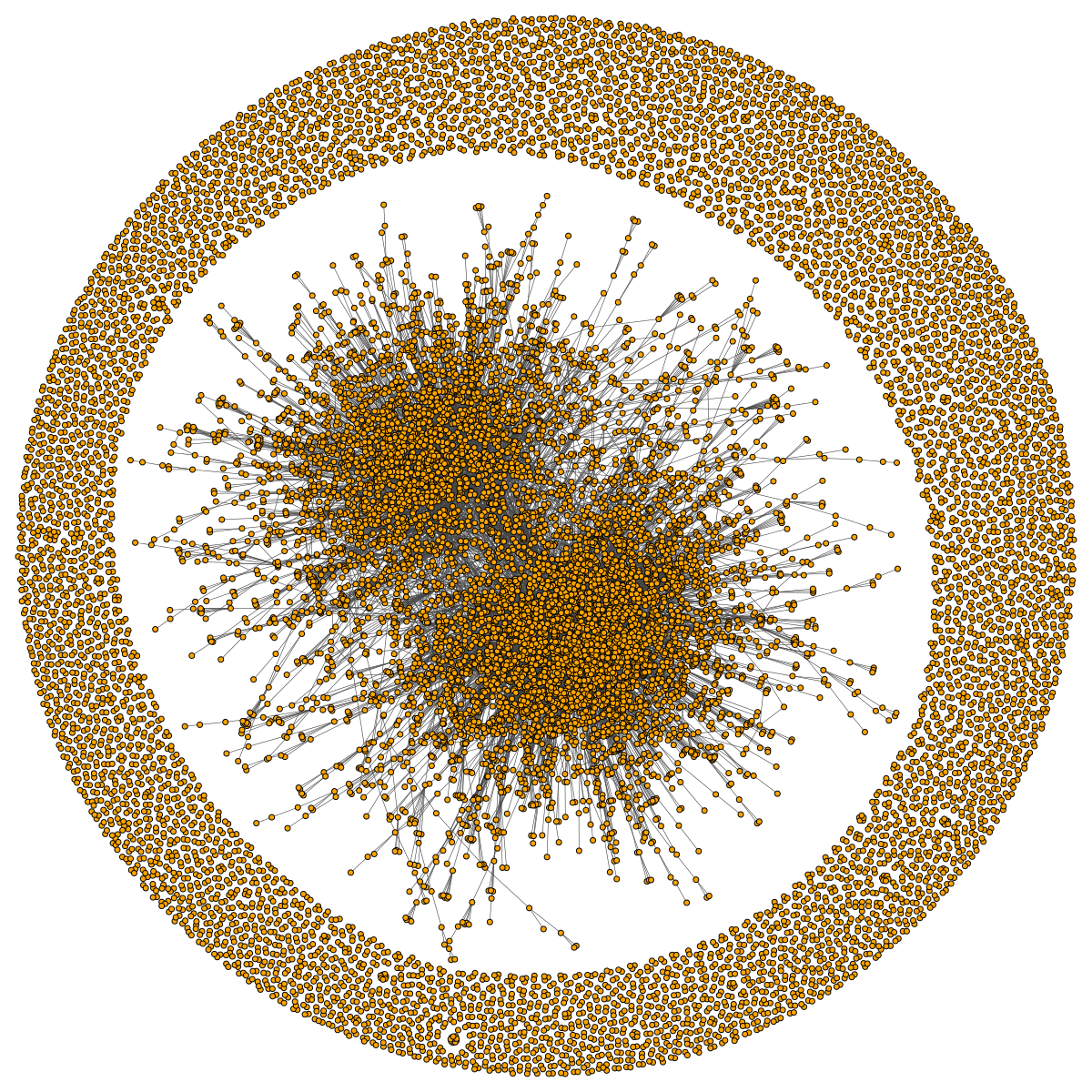
(a) (b)

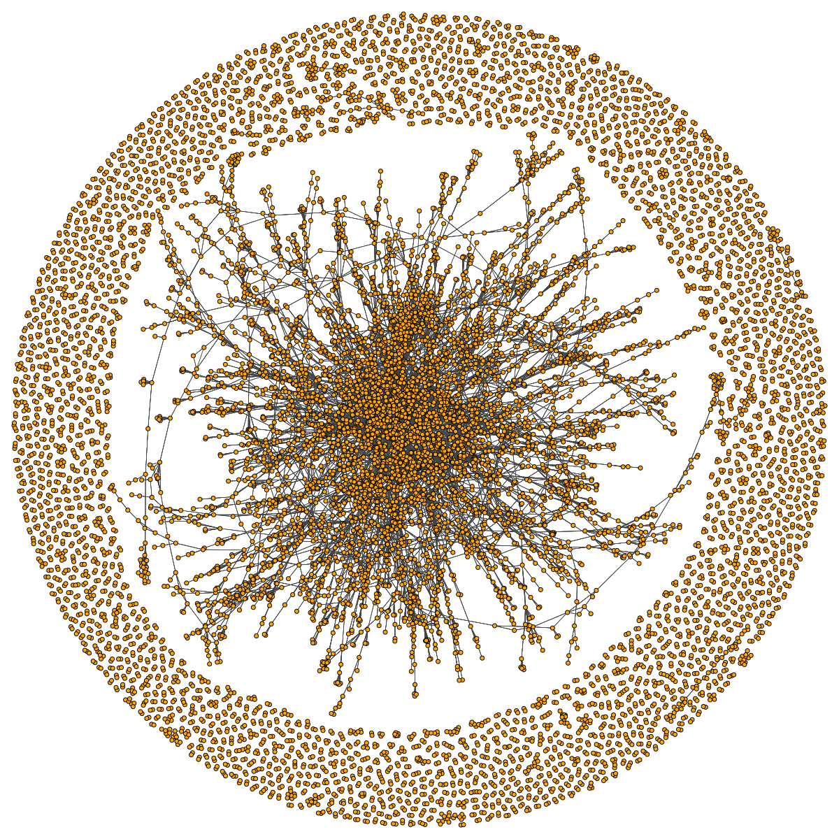
Figure 1: Visualization of collaboration networks: (left) R&D alliances of firms, (right) co-authorship relations of scientists. For the data sets see Section 3.1. We show the complete R&D network with about 14 000 nodes and 21 000 links, but only a sampled co-authorship network with about 11 000 nodes and 32 000 links (i.e. 10% of randomly chosen co-authors). For both networks we use the layout algorithm of fruchterman_reingold_1991.

2 Agent-based model of collaborations

How do economic actors or scientists choose their collaboration partners? At first, one would argue that scientists as decision makers are quite different from firms. In addition, inside their respective domain, how they choose partners may very much depend on the specific economic sector or scientific discipline. Thus, there is no ad-hoc evidence that such a problem can be addressed using the same modeling framework.

On the other hand, in order to reproduce a macroscopic structure such as a collaboration network, we may not need to include all the microscopic details that distinguish economic from social agents. Instead, an agent-based model should abstract from these details, to capture only the essential features of the decision making process. In this sense, we aim at an agent-based model that includes a minimalistic set of microscopic rules. We argue that this agent-based model is correct if it is able to reproduce a specific set of macroscopic properties of the different collaboration networks, namely degree distribution, path length distribution, distribution of community sizes, that are not used for the calibration of the model. At the same time, the agent-based model has to provide degrees of freedom to allow a proper calibration to reflect the differences of the domains in their respective empirical data.

In order to achieve this goal, this study utilizes a previously proposed agent-based model (tomasello2014therole) that has the above mentioned features. The model is flexible in that it builds on five probabilities to capture the choice of agents for collaborating with either established nodes or newcomers, which need to be calibrated. Obviously, different sets of probabilities may match the same macroscopic features. In order to distinguish between them, we adopt a Maximum-Likelihood approach that uses the mean degree, the mean path length, and the global clustering coefficient of the resulting collaboration network as quantities to be exactly matched.

In the model, agents represent nodes in a collaboration network and links between nodes represent collaboration events. Each agent is characterized by two individual attributes, activity $a_{i}$ and label $l_{i}$. Activity reflects the propensity to participate in a collaboration, while label indicates that the agent belongs to a group with a certain influence, discussed in detail below. The agent’s dynamics can be divided in two steps: first, the agent decides with whom to link, which impacts the network topology and the size of the network if a newcomer is chosen. Second, she adjusts her label, i.e. she keeps her previous label if she already has one, or she adopts the label of the counterparty if she is a newcomer, or she receives a new label, as discussed below.

Activation.

The model is initialized by assigning individual activities $a_{i}$ to agents which are sampled without replacement from the empirical distribution of activities (see Section 3.1). Hence, these activities are different for each agent and kept constant in time for the simulation. Next, at each time step, we select an agent to initiate a collaboration with probability $p_{i}$ proportional to its activity, $p_{i}=\eta a_{i}$, where $\eta$ is a rescaling parameter that we fix by imposing that $\sum_{i}p_{i}$ is equal to the number of collaboration event empirically observed per day.

Non-labeled versus labeled agents.

Activated agents can belong to two different groups: (a) newcomers, if they never engaged in a collaboration before, or (b) established agents, if they were already part of a previous collaboration. We distinguish between these groups by means of the agent label $l_{i}$. Newcomers are non-labeled, $l_{i}=0$, whereas established agents get a label depending on their first collaboration, $l_{i}>0$.

Collaboration size.

When an agent is activated, she initiates a collaboration. The number of partners for her collaboration, $m_{i}$, is obtained by sampling at random from the empirical size distribution of collaborating groups (see Section 3.1). The selection of partners is independent of the activity or other characteristics of the agent.

Collaboration partners.

Given the size of the collaboration, the initiator chooses partners either from the group of newcomers or from the group of established agents. This choice also depends on the label of the initiator herself and can be expressed by five probabilities. A labeled initiator links to another agent with the same label with probability $p^{L}_{s}$, to an agent with a different label with probability $p^{L}_{d}$, or to an agent without any label with probability $p^{L}_{n}$. If the initiator is a newcomer, i.e. non-labeled, she links to an labeled agent with probability $p^{N\!L}_{l}$ and to another newcomer with probability $p^{N\!L}_{n}$. Because the probabilities have to sum up to one, we have two constrains $p^{L}_{s}+p^{L}_{d}+p^{L}_{n}=1$ and $p^{N\!L}_{n}+p^{N\!L}_{l}=1$.

Link formation.

The probabilities to choose collaboration partners only consider the two groups, newcomers and established agents. To specify which of the specific agents from these groups are chosen, we adopt the preferential attachment rule. Precisely, the initiator $i$ selects, among all agents from the specific group, agent $j$ as collaborator with a probability proportional to the degree $k_{j}$ of $j$. If the initiator chooses a non-labeled agent ($k_{j}=0$) as collaborator, she will select uniformly at random from all non-labeled agents. After selecting the $m_{i}$ partners, we link all of them to the initiator, this way creating a clique of size $m+1$.

Label dynamics.

In our model, agents are initialized as non-labeled agents, i.e. they are considered as newcomers. An agent receives a label only when entering the network (which may consist of disconnected communities). This can happen in two different ways: either the agent initiates a collaboration, or the agent is chosen as partner by an activated agent. In the first case, the agent gets a new label assigned that was not used before. In the second case, the agent adopts the label from the initiator of the collaboration. The label is a unique attribute of an agent, i.e. once an agent has obtained a label, this cannot be changed.

Figure 2 summarizes the agent-based model described above. It illustrates the possible choices for the two different groups, newcomers and established agents. We note again that this choice progresses in three steps: First, activated agents choose ($m$ times) between newcomers and established agents as partners. Subsequently, if activated agents already have a label assigned, they have the choice between the group with the same label or groups with a different label. Finally, within the groups, agents choose their partners with respect to their degree. Obviously, the number of agents in each group and the degree of agents change dynamically as the network evolves.

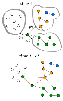
(a)   (b)

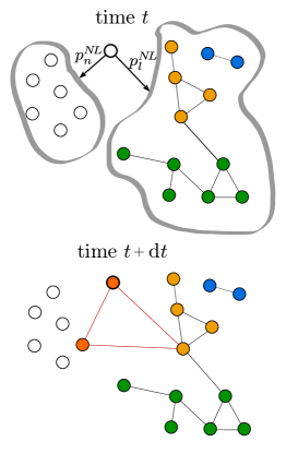
Figure 2: Two representative examples of collaboration selection and of label propagation. (a) A labeled agent (whose label is depicted in green) is activated at time $t$ and has to form an alliance with $m=2$ partners. She links to an agent having a different label (depicted in yellow) and one non-labeled, at time $t+\!dt$. (b) Likewise, a non-labeled agent gets activated at time $t\!$ and forms an alliance with $m=2$ partners. She links with one non-labeled agent and one labeled (yellow) agent at time $t\!+\!dt$.

3 Model calibration

3.1 Data sources

Our agent-based model, as already mentioned, will be calibrated and validated against data sets from two different domains, covering inter-firm R&D alliances and co-authorship of scientific papers. In the following, we describe the two data sets and afterwards how they are used as input for the model.

R&D network.

To reconstruct the R&D network of collaborating firms we use SDC Platinum database. It contains data about approximately 672,000 announced alliances from all countries between 1984 and 2009 with daily resolution. The economic actors participating in these alliances are of several types, e.g. investors, manufacturing firms and universities, but for simplicity we address them as firms. Each actor listed in the data set is associated with a SIC (Standard Industrial Classification) code that allows us to unambiguously assign its corresponding industrial sector. Further, the purpose of each alliance is characterized by various flags, e.g. manufacturing, licensing, research and development (R&D). We restrict ourselves to all alliances with the flag “R&D”, which gives us 14,829 alliances connecting 14,561 firms. The number of partners involved in each alliance can vary (see Section 3.2 for details). In most cases the alliance size is two, however it can also be three or higher.

In order to reconstruct the R&D network, we focus on the time-aggregated data set. Each firm engaged in a R&D alliance becomes a node and un-directed links connect nodes involved in the same alliance. By adopting this procedure, the 14,829 R&D alliances result in a total of 21,572 links connecting 14,561 nodes. To compare collaborations in different industrial sectors, we reconstruct six distinct R&D networks for the six largest industrial sectors. According to our data set, these are related to computer software, pharmaceuticals, R&D laboratory and testing, computer hardware, electronic components and communications equipment. An alliance is considered as part of a given sector if one of the collaborating firms has a matching SIC code. The details for the sectoral networks are given in Table 1. Additionally, we compare these sectoral networks with an aggregated R&D network, previously analyzed by tomasello2014therole, which was obtained by considering all the R&D alliances together, i.e. more than just the six largest industrial sectors.

Co-authorship network.

To reconstruct the collaboration network of scientists, we use the data set from the American Physical Society about papers published in any APS journal, namely Physical Review Letters, Reviews of Modern Physics, and all Physical Review journals. (APS). From this data set we use, for each publication, the names of the authors and PACS codes of the papers, to assign the publications to different research areas. We restrict ourselves to the period from 1983 to 2010, for which we use the time-aggregated data.

This data set has the limitation that the authors are identified by strings which often contain inconsistencies, e.g. missing special characters or spelling mistakes. Thus, in order to really make use of the APS data set, we have to disambiguate authors names in a separate, but time consuming, data processing. The latter involves matching the papers in the APS data set with Microsof Academic Search (MSAS) service, where both papers and authors have unique identifiers. The MSAS is a search engine which mines data from a bibliographic database containing information about scholars and their publications from 15 different disciplines. We have used the Application Programming Interface (API) of MSAS to obtain information about scholars publishing on APS. This way, we obtain a list of unique authors that we can use.

To reconstruct the co-authorship network, each unique author is represented by a node and links connect nodes that have co-authored at least one paper in the aggregated data set. Following this procedure, the 73,000 papers listed in the data set result in 300,000 links connecting 95,000 nodes.

At difference with the R&D networks, where firms are characterized by SIC codes, authors are not associated with any classification. Authors can change their research subject during their career, thus making a categorization on the author level difficult. Instead, the classification, i.e. the PACS number, is assigned to the links of the network representing the papers. For this reason, we build co-authorship networks of different fields by using the PACS numbers assigned to papers. In order to have co-authorship networks comparable in size and density with the R&D networks, we select the following six representative PACS numbers: 03 (quantum mechanics, field theories and special relativity), 04 (general relativity and gravitation) 42, (optics), 72 (electronic transport in condensed matter), 74 (superconductivity) and 89 (other areas of applied and interdisciplinary physics, that for example includes network theory). We report the sizes of these networks in Table 1.

	$N$	$E$	Links
Aggregated R&D network	14,561	14,829	21,572
Sectoral R&D networks
Pharmaceuticals (SIC 283)	3,829	5,277	6,019
Computer hardware (SIC 357)	1,582	2,672	4,047
Communications equipment (SIC 366)	1,133	1,888	2,726
Electronic components (SIC 367)	1,615	2,574	3,756
Computer software (SIC 737)	3,381	4,134	5,862
R&D, laboratory and testing (SIC 873)	3,188	4,032	5,364
Co-authorship networks
Quant. mech., field theories, spec. relativity (PACS 03)	21,501	19,647	56,111
General relativity and gravitation (PACS 04)	8,294	8,158	32,513
Optics (PACS 42)	27,436	20,105	94,961
Electronic transport in condensed matter (PACS 72)	19,492	11,687	55,818
Superconductivity (PACS 74)	14,920	10,541	52,615
Other applied and interdisciplin. physics (PACS 89)	4,881	2,873	8,777

Table 1: Number of nodes $N$, of collaboration events $E$ and of resulting links in our representation for the aggregated R&D network, the six largest sectoral R&D networks, and the six representative co-authorship networks. For all domains, we consider the respective cumulative networks, i.e. the networks obtained by keeping all the links at any time.

3.2 Input quantities

Based on the two data sets, we now calculate the two empirical inputs needed for our agent-based model, namely the size distribution of the collaboration events and the activity distribution of the agents.

Size of collaboration events.

In the SDC alliance data set, the size of a collaboration event is the number of firms per R&D alliance, while in the co-authorship data set it is the number of co-authors per paper. To study these, we analyzed the distributions of partners per collaboration event, $P(m)$, in both considered data sets.

With respect to our six sectoral R&D networks, we find that the size distribution is right-skewed with values ranging between 2 and 20. It should be noted that the identification of the functional form of these distributions (e.g., power-law, exponential, log-normal and so on) is outside of the scope of this study, therefore we leave it as a possible extension. Most of the collaborations are stipulated between two partners, but some alliances – the so-called consortia – involve three or more partners. In Figure 3 we report such distributions for two represetative industrial sectors. Results for four more industrial sectors are presented in Appendix A, confirming that the right-skewed distribution holds for all sectoral R&D networks, with only small differences in the tails of the respective distributions. These results are in line with the ones presented in (tomasello2014therole) for the aggregated R&D network.

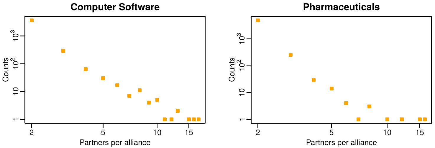
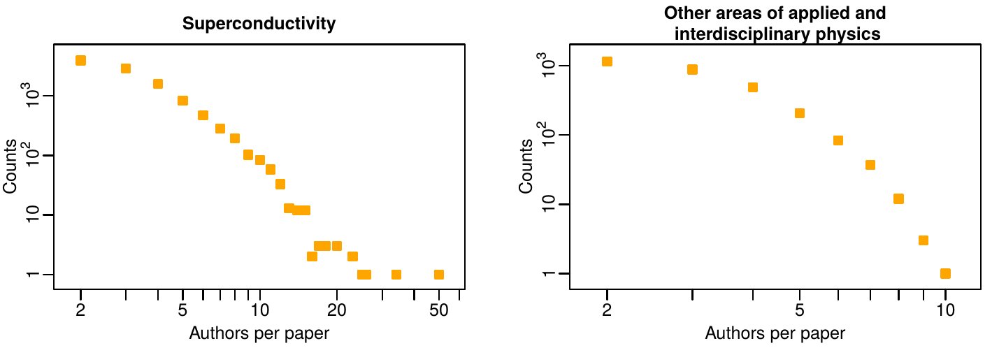
Figure 3: Distribution of the number of partners per alliance for two representative industrial sectors: computer software (top left)) and pharmaceutics (top right), as measured from the SDC data set. Distribution of the number of authors per paper for two representative co-authorship networks: superconductivity (bottom left) and interdisciplinary physics (bottom right), as measured from the APS-MSAS data set.

Regarding the size of scientific collaborations, we find results similar to the R&D alliances. I.e., most papers in our APS-MSAS data set have two co-authors with a broad right-skewed size distribution for all PACS numbers investigated. From our analysis, we have excluded all papers written by only one author because we are are interested in collaboration networks, where such papers would only generate isolated nodes. For this reason, the counts start from 2 in all of our plots. Figure 3 gives representative examples from two PACS numbers. Differently from the sectoral R&D networks, the co-authorship networks exhibit a larger degree of variability among PACS numbers. This is due to the fact that the typical number of authors per paper strongly depends on the field. To give an example, the field of applied and interdisciplinary physics is characterized by significantly fewer authors per paper (at most 10) than the field of general relativity and gravitation (whose right tail reaches 55 authors per paper). In Figure LABEL:fig:sectoral_partners and Figure LABEL:fig:authors_per_paper_distr in Appendix A, we show the distribution of collaboration sizes for respectively the six sectoral R&D networks and the six co-authorship networks.

Agents’ activity.

This is one of the two key attributes assigned to agents in our model. We apply a measure developed in the setting of temporal networks (holme2012temporal), which has been already used to analyze various data sets (barabasi2005origin; barabasi99:_emerg; pastor-satorras01:_dynam_correl_proper_inter), also in the context of R&D and co-authorship networks (tomasello2014therole; perra2012activity).

Following these approaches, we argue that activity reflects the propensity of an agent to participate in a collaboration event. Precisely, we define the empirical activity of an agent $i$ at time $t$ as the number of collaboration events, $e^{\Delta t}_{i,t}$, involving agent $i$ during a time window $\Delta t$ ending at time $t$ divided by the total number of collaboration events, $E^{\Delta t}_{t}$, involving any agent during the same period of time: $$a^{\Delta t}_{i,t}=\frac{{e^{\Delta t}_{i,t}}}{{E^{\Delta t}_{t}}}.$$ (1) For both the SDC alliance and APS-MSAS data sets, we measure the empirical distribution of activity, $P(a)$, for four different time windows, $\Delta t=1,5,10$ and 26. When the time window is shorter than 26 years (the entire data set observation period), we compute the activity by shifting the time window in 1-year increments and then we average the results. For simplicity, from now on, we will write $a^{\Delta t=26years}_{i,2009}$ as $a_{i}$, which is the activity over the longest time window. Interestingly, we find that these distributions are independent of the size of the time window, which is a robust feature for both R&D and co-authorship collaborations. In Figure 4, we report these results for two representative sectoral R&D networks and two representative co-authorship networks. For a visualization of the complete results for the six sectoral R&D networks see (tomasello2014therole) (Supplementary information) and for the six co-authorship networks see Figure LABEL:fig:coauthorship_activities in Appendix A.

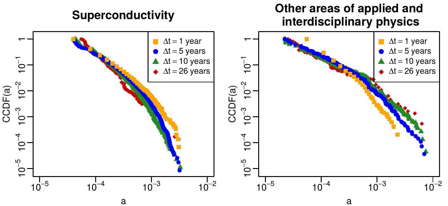
Figure 4: Complementary cumulative distribution function (CCDF) of the empirical firm activities, measured for two representative industrial sectors (from the SDC data set, (tomasello2014therole) Supplementary information), and of the empirical author activities, measured for two representative co-authorship networks (from the APS-MSAS data sets). We considered for 4 different time windows $\Delta t$ of 1, 5, 10 and 26 years.

3.3 Implementation and optimal model selection

To reproduce the collaboration networks from the two domains, we implement the agent-based model described in Section 2. For the simulations, we take the number of agents, $N$, and the total number of collaboration events, $E$, from the respective empirical networks. The two input parameters, size of the collaboration event, $m_{i}$, and agent activity, $a_{i}$, are obtained by sampling from the above distributions, $P(m)$ and $P(a)$. With that, the only free parameters in our model are the five probabilities $p_{s}^{L}$, $p_{d}^{L}$, $p_{n}^{L}$, $p_{n}^{NL}$, $p_{n}^{NL}$ which we vary in order to find which combination gives the best match between the simulated and the observed network. For more information about the exploration of the parameter space see Appendix B. For the comparison we use the following quantities: average degree, $\left\langle k\right\rangle$, average path length, $\left\langle l\right\rangle$, and global clustering coefficient, $C$, and define the respective relative errors $\varepsilon_{\left\langle k\right\rangle}$, $\varepsilon_{\left\langle l\right\rangle}$ and $\varepsilon_{C}$ between the observed and the simulated quantities. We require that these errors have to be smaller than a threshold $\varepsilon^{0}$. For all probability combinations we perform 25 simulations. We then select the combination that gives us the highest fraction of networks that match the criterion $\varepsilon<\varepsilon_{0}$. The optimal probabilities are indicated using a star (e.g. $p*_{s}^{L}$).

	$\quad p^{*L}_{s}$	$p^{*L}_{d}$	$p^{*L}_{n}$	$p^{*N\!L}_{l}$	$p^{*N\!L}_{nl}$
Aggregated R&D network	0.30	0.30	0.40	0.75	0.25
Sectoral R&D networks
Pharmaceuticals (SIC 283)	0.35	0.35	0.30	0.80	0.20
Computer hardware (SIC 357)	0.55	0.30	0.15	0.90	0.10
Communications equipment (SIC 366)	0.75	0.15	0.10	0.80	0.20
Electronic components (SIC 367)	0.65	0.20	0.15	0.90	0.10
Computer software (SIC 737)	0.55	0.20	0.25	0.95	0.05
R&D, laboratory and testing (SIC 873)	0.40	0.40	0.20	0.20	0.80
Co-authorship networks
Quant. mech., field theor., spec. relativity (PACS 03)	0.85	0.05	0.10	0.45	0.55
General relativity and gravitation (PACS 04)${}^{\dagger}{}$	0.50	0.05	0.45	0.05	0.95
Optics (PACS 42)	0.60	0.05	0.35	0.35	0.65
Electronic transport in condensed matter (PACS 72)	0.50	0.05	0.45	0.30	0.70
Superconductivity (PACS 74)	0.55	0.05	0.40	0.35	0.65
Other applied and interdisciplin. physics (PACS 89)	0.65	0.05	0.30	0.25	0.75

Table 2: Optimal sets of probabilities to simulated the collaboration networks. The optimal probabilities are indicated using ${}^{*}$. Recall that the probability of a labeled agent to select an agent with the same label is $p^{L}_{s}$, to select an agent with a different label is $p^{L}_{d}$) and to select a non-labeled agent is $p^{L}_{n}$). While, the probability of a non-labeled agent to select a labeled agent is $p^{N\!L}_{l}$ and to select a non-labeled agent is $p^{N\!L}_{nl}$. The probabilities $p^{L}_{s}$, $p^{L}_{d}$ and $p^{L}_{n}$ sum up to 1; likewise, $p^{N\!L}_{l}$ and $p^{N\!L}_{nl}$ sum up to 1.

${}^{\dagger}{}$ Only for the co-authorship network in general relativity and gravitation (PACS 04) the model is unable to generate a network matching all the three measures $\left\langle k\right\rangle$, $\left\langle l\right\rangle$ and $C$ at the same time. Only $\left\langle l\right\rangle$ and $C$ can be retrieved with an accuracy of 30%, while the generated $\left\langle k\right\rangle$ is not compatible with the empirical measure. Even though we report these values for completeness, they cannot be considered significant.

In Table 2 we report the optimal set of probabilities for the collaboration networks from the two different domains. The network simulated using the optimal set of probabilities will be named optimal simulated networks. In Table LABEL:table:collaboration_networks_empirical in Appendix B, we report the $\left\langle k\right\rangle$, $\left\langle l\right\rangle$ and $C$ of the optimal simulated networks and they can be compared with the respective values for the observed networks. With this, we are set for the validation of our agent-based model which of course has to include features of the network that were not used for the calibration of the model.

4 Model validation

4.1 Reproducing four distributions

To validate our agent-based model, we compare the empirical networks with the statistical properties of the simulated ones using the optimal set of probabilities. For the comparison, we use macroscopic features such as distributions of degrees, path lengths, local clustering coefficients and sizes of the disconnected components. Additionally, we also investigate microscopic, or agent centric, features such as labels. The validation procedure is similar to the one described in (tomasello2014therole). To validate the above mentioned distributions, we emphasize that for the calibration we did not use information about the distributions, but only about the respective average values, $\left\langle k\right\rangle$, $\left\langle l\right\rangle$ and $C$, to calculate the relative errors.

Figure 5 and Figure 6 show these distributions for one representative sectoral R&D network and one co-authorship network. We observe a remarkable match between the simulated and the empirical distributions for all four quantities. In particular, the model reproduces the emergence of a giant component in both networks, together with many smaller components down to size two.

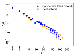
(a) (b)

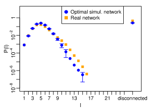
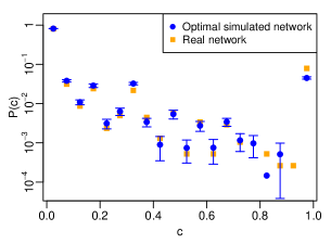
(c) (d)

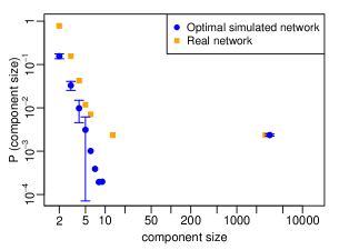
Figure 5: Distributions of node degrees (a), path lengths (b), local clustering coefficients (c) and component sizes (d) for the real and the 25 optimal simulated networks in “Pharmaceuticals”(SIC code 283). The blue circles in our plots correspond to the mean values and the error bars correspond to the standard deviations of all the quantities we analyze on the 25 realizations of each optimal simulated collaboration network. In many cases, the error bars are not visible, because the values are very narrowly distributed across these 25 realizations.

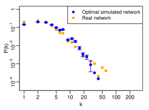
(a) (b)

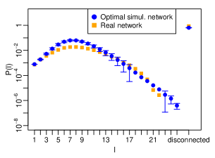
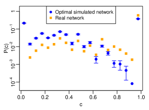
(c) (d)

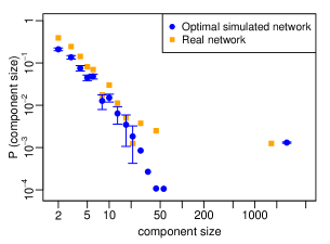
Figure 6: Distributions of node degrees (a), path lengths (b), local clustering coefficients (c) and component sizes (d) for the real and the 25 optimal simulated networks in applied and interdisciplinary physics (PACS number 89).

4.2 Community structures and groups of influence

The second part of our validation regards the modular structure of the collaboration networks in terms of communities. We start by evaluating and comparing the community structure of the observed networks and of the simulated ones using the optimal set of probabilities. Then, we verify that the groups of influence defined by the agents’ labels well reproduce the community structure of the simulated networks.

Community structure of empirical and simulated networks.

To detect the community structure in the observed networks, we employ a widely used algorithm, Infomap (rosvall2008infomap), which is based on the probability flow of random walks on networks. In Table LABEL:table:collaboration_networks_clusters in Appendix C, we report the number of communities found in each network. In Figure 7 (a), we give a visual representation of the respective communities in the co-authorship network in applied and interdisciplinary physics.

In order to quantify the goodness of the community partitions detected by Infomap, we use a normalized modularity score $Q$. This coefficient is equal to 1 when all links connect only nodes belonging to the same community, equal to 0 for a network where links are placed randomly, and equal to -1 when links are formed only among nodes populating distinct communities. Interestingly, we find that all the R&D and co-authorship networks are characterized by a high modularity as reported in Table LABEL:table:collaboration_networks_clusters in Appendix C. Precisely, all the $Q$ scores for partitions originated by Infomap are significantly higher than the equivalent scores on randomly generated networks with the same degree sequence, especially in the domain of co-authorship networks. We can safely conclude that our high $Q$ values are indicative of a real modular structure, and not a simple artifact of the network’s size and density(reichardt2006networks).

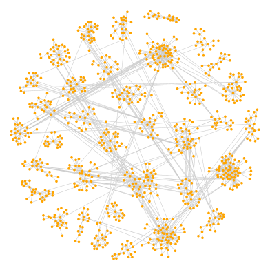
(a) (b)

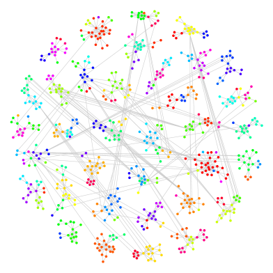
Figure 7: Co-authorship network in applied and interdisciplinary physics (PACS number 89).(a) Visual representation of the empirical network, considering only the 30 largest clusters detected by the Infomap algorithm. Distinct clusters are represented by grouping nodes in distinct regions of the plot area. (b) Visual representation of one realization of the simulated network, considering only the 30 largest clusters detected by the Infomap algorithm. Distinct clusters are represented by node groups in distinct regions of the plot area. In addition, we depict our node labels by using different colors: most of the nodes in a given cluster share the same label.

To detect communities structure on the simulated networks, we employ the same procedure we have described above. We visualize the partitioning detected for the co-authorship network in other applied and interdisciplinary physics in Figure 7 (b). The simulated distributions of clusters size match their empirical counterparts, which is far from being trivial given that no information about the community structure was used for the calibration. We report this result for the “Pharmaceuticals” R&D network in Figure 8 (a), and for the co-authorship network in applied and interdisciplinary physics in Figure 8 (b).

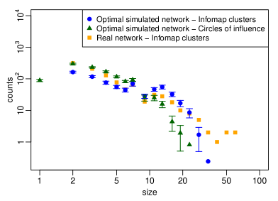
(a) (b)

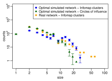
Figure 8: Size distribution of i. the circles of influence in the 25 realizations of the optimal simulated network, ii. the Infomap clusters in the 25 realizations of the optimal simulated network and iii. the Infomap clusters in the empirical network for “Pharmaceuticals” (SIC code 283) (a) and “Applied and interdisciplinary physics” (PACS number 89) (b).

Another evidence of their similarity is the modularity score of the optimal simulated networks – $Q^{*}=0.61\pm 0.01$ for the Pharmaceuticals R&D network, and $Q^{*}=0.87\pm 0.01$ for the co-authorship network in interdisciplinary physics. These values are close to their empirical equivalents, 0.62 and 0.92 respectively. In all cases, the modularity scores are significantly greater (with a $p$-value computationally indistinguishable from zero) than the ones obtained for a set of 100 randomly generated networks with the same degree sequence, proving that the obtained modularity cannot be expected or explained simply with the degree sequence.

Community structure using the agents’ labels.

In order to estimate the overlap between the communities detected using the Infomap algorithm and the group of influence defined by our agents’ labels, we use the normalized mutual information coefficient $I_{\mathrm{norm}}$ (danon2005comparing). We find that labels are actually able to reproduce the community structures of collaboration networks coming from both the economic and the scientific domains. $I_{\mathrm{norm}}(\mathrm{Labels,~{}Infomap~{}clusters})=0.887\pm 0.003$ for the “Pharmaceuticals” R&D network, and $I_{\mathrm{norm}}(\mathrm{Labels,~{}Infomap~{}clusters})=0.952\pm 0.002$ for the co-authorship network in interdisciplinary physics. This result is even more remarkable if we consider that the Infomap algorithm detects structural clusters based on the probability flow of random walks in the network, while our label propagation mechanism consists of an assignment of a fixed membership attribute – which is not only closer to a real phenomenon, but also computationally easier.

4.3 Distribution of path lengths at link formation

Finally, we compare the empirical and the simulated networks with respect to the distribution of path lengths between every pair of agents at the moment preceding the link formation. This is different from the distribution of path lengths analyzed before, which was computed on the time-aggregated networks. Now we are interested to know whether agents preferably form links with agents already part of the same connected component or with agents from another component or with newcomers. The respective distribution of link types is shown in Figure 9 for the “Pharmaceuticals” R&D network, and in Figure 10 for the co-authorship network in interdisciplinary physics. In all cases, there is a higher number of links with agents inside the same connected component or with newcomers. We emphasize the very good match between the empirical and the simulated frequencies of link types.

For links connecting agents which are already in the same connected component we can further discuss the network distance, or path length between two agents. It is interesting whether agents at larger network distances are still able to know each other and to form a link. Trivially, agents at distance 1 have already a collaboration (and can start a new one), whereas agents at distance 2 have one collaborator in common. We report our findings about the path length between agents before they engage in a collaboration in Figure 9 for the “Pharmaceuticals” R&D network, and in Figure 10 for the co-authorship network in interdisciplinary physics. We see that in the case of R&D networks agents preferably choose close collaborators for a new collaboration (path length up to 5), whereas for co-authorship networks agents prefer previous collaborators or collaborators at distance 2. In conclusion, the model correctly predicts the formation of links between agents no matter whether they are already in the same network component or not and gives an exact calculation of the shortest path length at the moment of link formation.

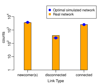
(a) (b)

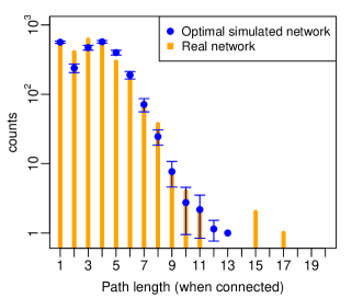
Figure 9: Temporal path length analysis for “Pharmaceuticals” R&D network (SIC code 283) . (a) Distribution of link types for empirical and simulated networks: “newcomer(s)” means that at least one of the agents was isolated (i.e. not yet part of the network) before the link formation; “disconnected” refers to agents already belonging to the network, but placed in two disconnected components; “connected” refers to agents already belonging to the same network component prior to the link formation. (b) Distribution of path lengths at the moment of link formation (only for agents belonging to the same connected component).

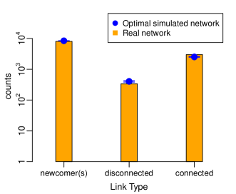
(a) (b)

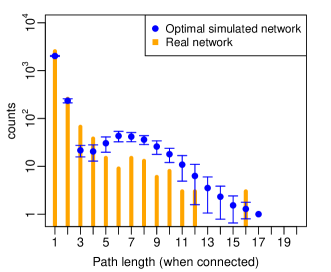
Figure 10: Temporal path length analysis for the co-authorship network in applied and interdisciplinary physics (PACS number 89) . (a) Distribution of link types for empirical and simulated networks: “newcomer(s)” means that at least one of the agents was isolated (i.e. not yet part of the network) before the link formation; “disconnected” refers to agents already belonging to the network, but placed in two disconnected components; “connected” refers to agents already belonging to the same network component prior to the link formation. (b) Distribution of path lengths at the moment of link formation (only for agents belonging to the same connected component).