Communication Complexity of Correlated Equilibrium in Two-Player Games
Abstract
We show a communication complexity lower bound for finding a correlated equilibrium of a two-player game. More precisely, we define a two-player game called the 2-cycle game and show that the randomized communication complexity of finding a -approximate correlated equilibrium of the 2-cycle game is . For small approximation values, this answers an open question of Babichenko and Rubinstein (STOC 2017). Our lower bound is obtained via a direct reduction from the unique set disjointness problem.
1 Introduction
If there is intelligent life on other planets, in a majority of them, they
would have discovered correlated equilibrium before Nash equilibrium.Roger Myerson
One of the most famous solution concepts in game theory is Nash equilibrium [Nas51]. Roughly speaking, a Nash equilibrium is a set of mixed strategies, one per player, from which no player has an incentive to deviate. A well-studied computational problem in algorithmic game theory is that of finding a Nash equilibrium of a given (non-cooperative) game. The complexity of finding a Nash equilibrium has been studied in several models of computation, including computational complexity, query complexity and communication complexity. Since finding a Nash equilibrium is considered a hard problem, researchers studied the problem of finding an approximate Nash equilibrium, where intuitively, no player can benefit much by deviating from his mixed strategy. For surveys on algorithmic game theory in general and equilibria in particular see for example [NRTV07, Rou10, Gol11, Rou16b].
A natural setting in which approximate equilibria concepts are studied is the setting of uncoupled dynamics [HMC03, HM06], where each player knows his own utilities and not those of the other players. The rate of convergence of uncoupled dynamics to an approximate equilibrium is closely related to the communication complexity of finding the approximate equilibrium [CS04].
Communication complexity is a central model in complexity theory that has been extensively studied. In the two-player randomized model [Yao79] each player gets an input and their goal is to solve a communication task that depends on both inputs. The players can use both common and private random coins and are allowed to err with some small probability. The communication complexity of a protocol is the total number of bits communicated by the two players. The communication complexity of a communication task is the minimal number of bits that the players need to communicate in order to solve the task with high probability, where the minimum is taken over all protocols. For surveys on communication complexity see for example [KN97, LS09, Rou16a].
In a recent breakthrough, Babichenko and Rubinstein [BR17] proved the first non-trivial lower bound on the randomized communication complexity of finding an approximate Nash equilibrium.
An important generalization of Nash equilibrium is correlated equilibrium [Aum74, Aum87]. Whereas in a Nash equilibrium the players choose their strategies independently, in a correlated equilibrium the players can coordinate their decisions, choosing a joint strategy. Babichenko and Rubinstein [BR17] raised the following questions:
Does a communication protocol
for finding an approximate correlated equilibrium of two-player games exist?
Is there a communication complexity lower bound?
We answer these questions for small approximation values. As far as we know, prior to this work, no non-trivial answers were known (neither positive nor negative), not even for the problem of finding an exact correlated equilibrium of two-player games. In contrast, in the multi-party setting, there is a protocol for finding an exact correlated equilibrium of -player binary action games with bits of communication [HM10, PR08, JL15].
There are two notions of correlated equilibrium which we call correlated and rule correlated equilibria. In a correlated equilibrium no player can benefit from replacing one action with another, whereas in a rule correlated equilibrium no player can benefit from simultaneously replacing every action with another action (using a switching rule). While the above two notions are equivalent, approximate correlated and approximate rule correlated equilibria are not equivalent, but are closely related.
Our first communication complexity lower bound is for finding a -approximate correlated equilibrium of a two-player game called the 2-cycle game. We note that every two-player game has a trivial -approximate correlated equilibrium (which can be found with zero communication).
Theorem 1.1.
For every , every randomized communication protocol for finding an -approximate correlated equilibrium of the 2-cycle game, with error probability at most , has communication complexity at least .
Since every approximate rule correlated equilibrium is an approximate correlated equilibrium, the following lower bound follows from Theorem 1.1. It remains an interesting open problem to prove bounds on the communication complexity of finding a constant approximate rule correlated equilibrium of two-player games.
Theorem 1.2.
For every , every randomized communication protocol for finding an -approximate rule correlated equilibrium of the 2-cycle game, with error probability at most , has communication complexity at least .
Note that Theorems 1.1 and 1.2 imply a lower bound of for the randomized query complexity of finding a -approximate correlated, respectively rule correlated, equilibrium of the 2-cycle game on actions.
Next, we show a communication complexity lower bound for finding a -approximate Nash equilibrium of the 2-cycle game. As previously mentioned, Babichenko and Rubinstein [BR17] proved the first non-trivial lower bound on the randomized communication complexity of finding an approximate Nash equilibrium. More precisely, they proved a lower bound of on the randomized communication complexity of finding an -approximate Nash equilibrium of a two-player game, for every , where is some small constant. Their proof goes through few intermediate problems and involves intricate reductions. We believe our proof is more simple and straightforward. Moreover, for small approximation values, we get a stronger lower bound of , as opposed to the lower bound of [BR17].
Theorem 1.3.
For every , every randomized communication protocol for finding an -approximate Nash equilibrium of the 2-cycle game, with error probability at most , has communication complexity at least .
Using similar ideas to the ones used in the proof of Theorem 1.3, we get a communication complexity lower bound for finding an approximate well supported Nash equilibrium of the 2-cycle game.
Theorem 1.4.
For every , every randomized communication protocol for finding an -approximate well supported Nash equilibrium of the 2-cycle game, with error probability at most , has communication complexity at least .
The 2-cycle game is a very simple game, in the sense that it is a win-lose, sparse game, in which each player has a unique best response to every action. Moreover, the 2-cycle game has a unique pure Nash equilibrium, hence the non-deterministic communication complexity of finding a Nash or correlated equilibrium of the 2-cycle game is .
The construction of the utility functions of the 2-cycle game was inspired by the gadget reduction of [RW16] which translates inputs of the fixed-point problem in a compact convex space to utility functions. However, the utility functions of the 2-cycle game are defined using the unique out-neighbor function on a directed graph.
Our lower bounds are obtained by a direct reduction from the unique set disjointness problem. We show that the randomized communication complexity of finding the pure Nash equilibrium of the 2-cycle game is and that given an approximate Nash or correlated equilibrium of the 2-cycle game, the players can recover the pure Nash equilibrium with small amount of communication. Note that for small approximation values, Theorems 1.1–1.4 are tight for the class of win-lose, sparse games, up to logarithmic factors, as a player can send his entire utility function using bits of communication.
Based on the 2-cycle game, we define a Bayesian game for two players called the Bayesian 2-cycle game. This is done by splitting the original game into smaller parts, where each part corresponds to a type and is in fact a smaller 2-cycle game. The players are forced to play the same type each time, hence the problem of finding an approximate Bayesian Nash equilibrium of this game is essentially reduced to the problem of finding an approximate Nash equilibrium of the 2-cycle game. For a constant , Theorem 1.5 gives a tight lower bound of for finding a constant approximate Bayesian Nash equilibrium of the Bayesian 2-cycle game on types.
Theorem 1.5.
Let and . Then, for every , every randomized communication protocol for finding an -approximate Bayesian Nash equilibrium of the Bayesian 2-cycle game on actions and types, with error probability at most , has communication complexity at least .
We note that our results do not hold for much larger approximation values, since there are examples of approximate equilibria of the 2-cycle game for larger approximation values, that can be found with small amount of communication (see Appendix A for details). We discuss some of the remaining open problems in Section 6.
1.1 Related Works
We overview previous works related to the computation of Nash and correlated equilibria of two-player games.
Computational complexity.
The computational complexity of finding a Nash equilibrium has been extensively studied in literature. Papadimitriou [Pap94] showed that the problem is in \PPAD, and over a decade later it was shown to be complete for that class, even for inverse polynomial approximation values [DGP09, CDT09]. However, for constant approximation values, Lipton et al. [LMM03] gave a quasi-polynomial time algorithm for finding an approximate Nash equilibrium, and this was shown to be optimal by Rubinstein [Rub16] under an ETH assumption for \PPAD. In stark contrast, exact correlated equilibrium can be computed for two-player games in polynomial time by a linear program [HS89]. The decision version of finding Nash and correlated equilibria with particular properties have also been considered in literature (for examples see [GZ89, CS08, ABC11, BL15, DFS16]). Finally, we note that Rubinstein [Rub15] showed that finding a constant approximate Nash equilibrium of Bayesian games is \PPAD-complete.
Query complexity.
[FS16] showed a lower bound of on the deterministic query complexity of finding an -approximate Nash equilibrium, where . In the other direction, [FGGS15] showed a deterministic query algorithm that finds a -approximate Nash equilibrium by making queries. For randomized query complexity, [FS16] showed a lower bound of for finding an -approximate Nash equilibrium, where . In the other direction, [FS16] showed a randomized query algorithm that finds a -approximate Nash equilibrium by making queries. For coarse correlated equilibrium, Goldberg and Roth [GR14] provided a randomized query algorithm that finds a constant approximate coarse correlated equilibrium by making queries.
Communication complexity.
The study of the communication complexity of finding a Nash equilibrium was initiated by Conitzer and Sandholm [CS04], where they showed that the randomized communication complexity of finding a pure Nash equilibrium (if it exists) is . On the other hand, [GP14] showed a communication protocol that finds a 0.438-approximate Nash equilibrium by exchanging bits of communication, and [CDF+16] showed a communication protocol that finds a 0.382-approximate Nash equilibrium with similar communication. In a recent breakthrough, Babichenko and Rubinstein [BR17] proved the first lower bound on the communication complexity of finding an approximate Nash equilibrium. They proved that there exists a constant , such that for all , the randomized communication complexity of finding an -approximate Nash equilibrium is at least . Note that before [BR17] no communication complexity lower bound was known even for finding an exact mixed Nash equilibrium.
1.2 Proof Overview
The 2-cycle game is defined on two directed graphs, one for each player, where both graphs have a common vertex set of size . The actions of each player are the vertices. The utility of a pair of vertices for a player is 1 if he plays the unique out-neighbor (according to his graph) of the vertex played by the other player, otherwise it is 0.
Each graph is constructed from a subset of , such that the two subsets have exactly one element in common. The union of the two graphs has a unique 2-cycle that corresponds to the element in the intersection of the subsets. We show that the 2-cycle game has a unique pure Nash equilibrium, that also corresponds to the 2-cycle in the union of the graphs. Since it is hard to find the element in the intersection of the subsets, finding the pure Nash equilibrium of the 2-cycle game is also hard.
Next, we show that each player can extract from an approximate correlated equilibrium a partial mixed strategy on his actions, by looking at the edges of his graph. We show that the partial strategies are either concentrated on the pure Nash equilibrium or one of these partial strategies has an unusual probability on a vertex which is closely related to the pure Nash equilibrium.
Assuming that the latter does not hold, we show that the partial strategies are concentrated on the pure Nash equilibrium as follows: The union of the two graphs is a layered graph with layers. In that graph there is a path of length that ends at the 2-cycle. Using a delicate analysis of the structure of the graph, we prove inductively, moving forward along the path, that the players play the vertices along the path (up to but not including the 2-cycle) with small probability. Since the partial strategies hold a meaningful weight of the correlated distribution, they must be concentrated on the 2-cycle, i.e. the pure Nash equilibrium.
Given these partial strategies, the players can recover the pure Nash equilibrium with small amount of communication. The lower bound then follows from the hardness of finding the pure Nash equilibrium of the 2-cycle game.
The proof of the lower bound for finding an approximate Nash equilibrium is very similar, however it does not require such a delicate analysis.
2 Preliminaries
2.1 General Notation
Strings.
For two bit strings , let be the concatenation of and . For a bit string and an index , is the bit in and is the negated bit string, that is is the negation of .
Probabilities of sets.
For a function , where is some finite set, and a subset , let . Define and . For a function , where are some finite sets, and a subset , let . For a subset and , let . Similarly, for a subset and let .
Conditional distributions.
For a distribution over , where are some finite sets, and let be the distribution over defined as
Similarly, for let be the distribution over defined as
2.2 Win-Lose and Bayesian Games
A win-lose, finite game for two players and is given by two utility functions and , where and are finite sets of actions. We say that the game is an game, where . A mixed strategy for player is a distribution over and a mixed strategy for player is a distribution over . A mixed strategy is called pure if it has only one action in its support. A correlated mixed strategy is a distribution over . A switching rule for player is a mapping from to and a switching rule for player is a mapping from to .
A Bayesian, finite game for two players and is given by a distribution over and two utility functions and , where , are finite sets of actions, and , are finite sets of types. We say that the game is on actions and types where and . A mixed strategy for player is a distribution over and a mixed strategy for player is a distribution over . A mixed strategy is called pure if it has only one action in its support.
2.3 Approximate Correlated Equilibrium
Definition 2.1.
Let . An -approximate correlated equilibrium of a two-player game is a correlated mixed strategy such that the following two conditions hold:
-
1.
For every actions ,
-
2.
For every actions ,
Definition 2.2.
Let . An -approximate rule correlated equilibrium of a two-player game is a correlated mixed strategy such that the following two conditions hold:
-
1.
For every switching rule for player ,
-
2.
For every switching rule for player ,
When the approximation value is zero, the two notions above coincide. The following proposition states that every approximate rule correlated equilibrium is an approximate correlated equilibrium.
Proposition 2.3.
Let and let be an -approximate rule correlated equilibrium of a two-player game. Then, is an -approximate correlated equilibrium of the game.
Proof.
Assume towards a contradiction that is not an -approximate correlated equilibrium. Then, without loss of generality, there exist actions such that
Define a switching rule for player as follows:
Then, for every and , it holds that . Therefore,
which is a contradiction. ∎
In the other direction, the following holds.
Proposition 2.4.
Let and let be an -approximate correlated equilibrium of an action two-player game. Then, is an -approximate rule correlated equilibrium of the game.
Proof.
Assume towards a contradiction that is not an -approximate rule correlated equilibrium. Then, without loss of generality, there exists a function such that
From an averaging argument, there exists such that
which is a contradiction. ∎
The Communication Task
The communication task of finding an -approximate (rule) correlated equilibrium is as follows. Consider a win-lose, finite game for two players and , given by two utility functions and .
The inputs:
The actions sets and the approximation value are known to both players. Player gets the utility function and player gets the utility function . The utility functions are given as truth tables of size each.
At the end of the communication:
Both players know the same correlated mixed strategy over , such that is an -approximate (rule) correlated equilibrium.
2.4 Approximate Nash Equilibrium
Definition 2.5.
Let . An -approximate Nash equilibrium of a two-player game is a pair of mixed strategies for the players respectively, such that the following two conditions hold:
-
1.
For every mixed strategy for player ,
-
2.
For every mixed strategy for player ,
An approximate Nash equilibrium with is called an exact Nash equilibrium. A two-player game has a pure Nash equilibrium , where and , if there exists an exact Nash equilibrium , where the support of is and the support of is .
Definition 2.6.
Let . An -approximate well supported Nash equilibrium of a two-player game is a pair of mixed strategies for the players respectively, such that the following two conditions hold:
-
1.
For every action and every action ,
-
2.
For every action and every action ,
When the approximation value is zero, the two notions above coincide. The following proposition states that every approximate well supported Nash equilibrium is an approximate Nash equilibrium.
Proposition 2.7.
Let and let be an -approximate well supported Nash equilibrium of a two-player game. Then, is an -approximate Nash equilibrium of the game.
Proof.
Let be a mixed strategy for player . For every action and every action ,
Therefore,
Similarly, for every mixed strategy for player , every action and every action ,
Therefore,
∎
The Communication Task
The communication task of finding an -approximate (well supported) Nash equilibrium Consider a win-lose, finite game for two players and , given by two utility functions and .
The inputs:
The actions sets and the approximation value are known to both players. Player gets the utility function and player gets the utility function . The utility functions are given as truth tables of size each.
At the end of the communication:
Player knows a mixed strategy over and player knows a mixed strategy over , such that is an -approximate (well supported) Nash equilibrium.
2.5 Approximate Bayesian Nash Equilibrium
Definition 2.8.
An -approximate Bayesian Nash equilibrium of a two-player game is a set of mixed strategies for player and a set of mixed strategies for player such that the following two conditions hold:
-
1.
For every type and every mixed strategy for player ,
-
2.
For every type and every mixed strategy for player ,
The Communication Task
The communication task of finding an -approximate Bayesian Nash equilibrium Consider a Bayesian, finite game for two players and , on actions and types, that is given by the distribution over and the two utility functions and .
The inputs:
All the sets , the distribution and the approximation value are known to both players. Player gets the utility function and player gets the utility function . The utility functions are given as truth tables of size at most each.
At the end of the communication:
Player knows a set of mixed strategies and player knows a set of mixed strategies , such that is an -approximate Bayesian Nash equilibrium.
3 The 2-Cycle Game
Let , . The 2-cycle game is constructed from two -bit strings for which there exists exactly one index , such that . Throughout the paper, all operations (adding and subtracting) are done modulo .
The graphs.
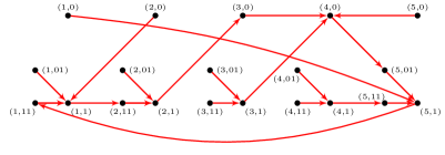
Given a string , player computes the graph on the set of vertices with the following set of directed edges (an edge is directed from into ):
See an example of such a graph in Figure 1.
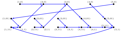
Given a string , player computes the graph on the same set of vertices with the following set of directed edges:
See an example of such a graph in Figure 2.
The actions and utility functions.
The sets of actions are . The utility function of player is defined for every pair of actions as
The utility function of player is defined for every pair of actions as
This is a win-lose, game, where . We call it the 2-cycle game or more specifically, the 2-cycle game.
3.1 Notations
For two vertices , is a 2-cycle if and . For a vertex , define
That is, is the set of incoming neighbors to in , and is the set of incoming neighbors to in . Let and . For a subset , define
For every , layer is the set of vertices defined as
Another useful set of vertices is a midway layer defined as
Edges in of the form for are called back-edges. For a vertex , define
For a subset , define
Let be the strings from which the game was constructed. Note that determines , and determines . For an index we say that is disputed if . Otherwise, we say that is undisputed. Define to be the unique disputed index. We denote the following key vertices:
For , and a function , we say that is -concentrated on if
To simplify notations, for a function taking inputs from the set and a vertex , we write instead of .
3.2 Basic Properties
The following are some useful, basic properties of the 2-cycle game.
Proposition 3.1 (Out-degree).
For every , there exists exactly one such that . Similarly, for every , there exists exactly one such that .
Proof.
Follows immediately from the definitions of and . ∎
Proposition 3.2 (Max in-degree).
For every , it holds that and .
Proof.
Follows immediately from the definitions of and . ∎
By the following claim, the 2-cycle game has exactly one 2-cycle.
Proposition 3.3 (A 2-cycle).
Let be a back-edge. If , then . Otherwise, and is a 2-cycle.
Proof.
Let , for some and assume there exits , for some . By the definition of ,
If , then and by the definition of , . Otherwise and . Since it holds that . Since it holds that and by the definition of , . ∎
3.3 Pure Nash Equilibrium
By Claim 3.4 below, the 2-cycle game has a unique pure Nash equilibrium. Together with Proposition 3.3, the pure Nash equilibrium of the game is its 2-cycle.
Claim 3.4.
The 2-cycle game has exactly one pure Nash equilibrium .
Proof.
By Proposition 3.3, is a 2-cycle. That is, and . Let be the mixed strategy for player with support and be the mixed strategy for player with support . Then,
For every mixed strategy for player it holds that
Similarly, for every mixed strategy for player ,
Therefore, is a pure Nash equilibrium.
Let such that or .
Let be the mixed strategy for player with support and
be the mixed strategy for player with support .
By Proposition 3.3, either or .
By proposition 3.1,
there exist such that and .
If then let be the mixed strategy for player with support .
We get that
and
Otherwise , then let be the mixed strategy for player with support . We get that
and
Therefore, is not a pure Nash equilibrium. ∎
The following theorem states that finding the pure Nash equilibrium (equivalently, the 2-cycle) of the 2-cycle game is hard. The proof is by a reduction from the following search variant of unique set disjointness: Player gets a bit string and player gets a bit string . They are promised that there exists exactly one index such that . Their goal is to find the index . It is well known that the randomized communication complexity of solving this problem with constant error probability is [BFS86, KS92, Raz92]. This problem is called the universal monotone relation. For more details on the universal monotone relation and its connection to unique set disjointness see [KN97].
Theorem 3.5.
Every randomized communication protocol for finding the pure Nash equilibrium of the 2-cycle game, with error probability at most , has communication complexity at least .
Proof.
Let be the inputs to the search variant of unique set disjointness described above. Consider the 2-cycle game which is constructed from these inputs, given by the utility functions . Assume towards a contradiction that there exists a communication protocol for finding the pure Nash equilibrium of the 2-cycle game with error probability at most and communication complexity . The players run on and with probability at least , at the end of the communication, player knows and player knows , such that is the pure Nash equilibrium of the game. By Claim 3.4, and . Given to the players and respectively, both players know the index , which is a contradiction. ∎
4 Approximate Correlated Equilibrium of The 2-Cycle Game
The following theorem states that given an approximate correlated equilibrium of the 2-cycle game, the players can recover the pure Nash equilibrium.
Theorem 4.1.
Consider a 2-cycle game, given by the utility functions . Let and let be an -approximate correlated equilibrium of the game. Then, there exists a deterministic communication protocol, that given , to player , and , to player , uses bits of communication, and at the end of the communication player outputs an action and player outputs an action , such that is the pure Nash equilibrium of the game.
Theorem 1.1 follows from Theorem 3.5 and Theorem 4.1. For the rest of this section we prove Theorem 4.1. The proof uses the notion of slowly increasing probabilities. For more details on slowly increasing probabilities see Section 4.1.
Definition 4.2 (Slowly increasing probabilities).
Let . A pair of functions and is -slowly increasing for the 2-cycle game if for every the following conditions hold:
-
1.
.
-
2.
.
In particular, if then . Similarly, if then .
The next lemma states that given a pair of functions which is -slowly increasing for the 2-cycle game, for a small enough , the players can recover the pure Nash equilibrium. The proof is in Section 4.2
Lemma 4.3.
Consider a 2-cycle game, given by the utility functions . Let and be a pair of functions which is -slowly increasing for the game, where . Then, there exists a deterministic communication protocol, that given , and to player , and , and to player , uses bits of communication, and at the end of the communication player outputs an action and player outputs an action , such that is the pure Nash equilibrium of the game.
We prove that an approximate correlated equilibrium for the 2-cycle game implies the existence of a slowly increasing pair of functions. Theorem 4.1 follows from Lemma 4.3 and Claim 4.4.
Claim 4.4.
Let be an -approximate correlated equilibrium of the 2-cycle game, where . Then, there exists a pair of functions and which is -slowly increasing for the game. Moreover, player knows , player knows and .
Proof.
Define a function as
and a function as
Let and assume that for some . We will show that . Let (if there is no such vertex we are done). By Definition 2.1, for every ,
By Proposition 3.1, there exists such that . Therefore,
Summing over every we get that
where we bounded the left-hand side by Proposition 3.2
and the right-hand side by the assumption.
The same holds when replacing with , with , and with .
That is, for every , if for some ,
then .
Finally, we bound :
where the first step follows from the definition of and from Proposition 3.1 and the second step follows from Definition 2.1. Therefore, . ∎
4.1 On Slowly Increasing Probabilities
In this section we describe some useful, basic properties of slowly increasing probabilities for the 2-cycle game.
Recall that for a vertex , is the set of vertices such that but is not a back-edge. The following proposition states that a back-edge adds at most to the probability of its vertices.
Proposition 4.5.
Let and let and be a pair of functions which is -slowly increasing for the 2-cycle game. Let , where , and . Then .
Proof.
Recall that for , . The following proposition states that bounding the probabilities of vertices in a midway layer implies a bound on the corresponding layer.
Proposition 4.6.
Let and let and be a pair of functions which is -slowly increasing for the 2-cycle game. Let such that . Then,
Recall that an index is disputed if , where are the strings from which the game was constructed, otherwise is undisputed. The game has exactly one disputed index .
Proposition 4.7.
Let and let and be a pair of functions which is -slowly increasing for the 2-cycle game. Let be the strings from which the game was constructed. For every , if is undisputed and then .
Proof.
Let and assume that is undisputed and . There are exactly two edges in going into , from the vertices and . Since is undisputed, and . By Definition 4.2,
∎
4.2 From Slowly Increasing Probabilities to The Pure Nash Equilibrium
In this section we prove Lemma 4.3. Consider a 2-cycle game, given by the utility functions . Let and be a pair of functions which is -slowly increasing for the game, where . By Claim 3.4, the pure Nash equilibrium of the game is .
The deterministic communication protocol for finding is described in Algorithm 1. Player gets , and and player gets , and . The communication complexity of this protocol is clearly at most .
-
1.
Player checks if there exists such that and . If there is such an index he sends it to player . Then, player outputs and player outputs . Otherwise, player sends a bit to indicate that there is no such index.
-
2.
Player checks if . If it is, player finds such that , where and , and sends to player . Then, player outputs and player outputs . Otherwise, player sends a bit to indicate that .
-
3.
Player finds such that , where and , and sends to player . Then, player outputs and player outputs .
By Proposition 4.7, if there exists such that and , then has to be . In this case the players output and respectively. Otherwise, . In this case, the correctness of the protocol follows from Lemma 4.8 below.
Lemma 4.8.
Consider a 2-cycle game, given by the utility functions . Let and be a pair of functions which is -slowly increasing for the game, where . Let . Then, either or the following two conditions hold:
-
1.
is -concentrated on .
-
2.
is -concentrated on .
Note that if then and . Otherwise, then and . For the rest of this section we prove Lemma 4.8. Assume that . First, note that therefore
and by Proposition 4.5,
Next, we prove that for every ,
| (1) |
Recall that . By Proposition 4.6, (1) implies that for every . Note that . We prove (1) by induction on , from to .
Layer :
First we bound . Note that in there is no edge from to or to . Moreover, by Proposition 3.1, every vertex has exactly one out-going edge in each graph. That is, in , either there is an edge from to or there is an edge from to , but not both. Therefore,
where the first step follows from Definition 4.2, Proposition 4.5 and since .
Next we bound .
In , either there are edges from and to and respectively,
or there are edges from and to , but not both.
Therefore, by Definition 4.2,
Put together we get that .
Layers :
Fix . By Proposition 3.1, every vertex has exactly one out-going edge in each graph. That is, in each graph, either and have no incoming edges from layer , or has no incoming edges from layer . If and have no incoming edges from layer in then
where the first step holds since and the second step follows from Proposition 4.5. Otherwise, has no incoming edges from layer in and then
where the first step follows from Proposition 4.5
since
and the second step follows from Definition 4.2.
The same holds when replacing with , and with .
(the fact that there are no back-edges in could only decrease the bound).
That is,
| (2) |
Put together we get that
Assume that and that (1) holds for every . By Proposition 4.6, for every . Therefore,
Bounding on the remaining vertices.
It remains to bound on the vertices , where . It holds that
where the first step follows from (2), the second step follows from Proposition 4.6 and the third step follows from (1). Finally,
where the first two steps follow from Definition 4.2, the third step follows from Proposition 4.6 and fourth step follows from (1).
Bounding on the remaining vertices.
We already bounded on the vertices and . It remains to bound on the vertices and . Denote . Since there is not back-edge into ,
where the first two steps follow from Definition 4.2, the third step follows from Proposition 4.6 and fourth step follows from (1). Finally,
where the first three steps follow from Definition 4.2, the fourth step follows from Proposition 4.6 and the fifth step follows from (1).
5 Approximate Nash Equilibrium of The 2-Cycle Game
The following theorem states that given an approximate Nash equilibrium of the 2-cycle game, the players can recover the pure Nash equilibrium.
Theorem 5.1.
Consider a 2-cycle game, given by the utility functions . Let and let be an -approximate Nash equilibrium of the game. Then, there exists a deterministic communication protocol, that given , to player , and , to player , uses bits of communication, and at the end of the communication player outputs an action and player outputs an action , such that is the pure Nash equilibrium of the game.
Theorem 1.3 follows from Theorem 3.5 and Theorem 5.1. For the rest of this section we prove Theorem 5.1. The proof uses the notion of non-increasing probabilities. For more details on non-increasing probabilities see Section 5.1.
Definition 5.2 (Non-increasing probabilities).
Let . A pair of distributions , each over the set of actions , is -non-increasing for the 2-cycle game if for every the following conditions hold:
-
1.
If then .
-
2.
If then .
In particular, if then and therefore . Similarly, if then .
The next lemma states that given a pair of distributions which is -non-increasing for the 2-cycle game, for a small enough , the players can recover the pure Nash equilibrium. The proof is in Section 5.2
Lemma 5.3.
Consider a 2-cycle game, given by the utility functions . Let be a pair of distributions, each over the set of actions , which is -non-increasing for the game, where . Then, there exists a deterministic communication protocol, that given , and to player , and , and to player , uses at most bits of communication, and at the end of the communication player outputs an action and player outputs an action , such that is the pure Nash equilibrium of the game.
We prove that an approximate Nash equilibrium for the 2-cycle game is a non-increasing pair of functions. Theorem 5.1 follows from Lemma 5.3 and Claim 5.4.
Claim 5.4.
Let be an -approximate Nash equilibrium of the 2-cycle game, where . Then, the pair is -non-increasing for the game.
Proof.
Let and assume that for every . Let be a vertex such that (there must exist such a vertex since is a distribution). By Proposition 3.1, there exists a vertex such that . Note that by our assumption, and . Define a distribution over as follows:
By Definition 2.5,
where the last step follows from Proposition 3.2.
Since we conclude that .
The same holds when replacing with , with , and with .
That is, for every , if for every
then .
∎
5.1 On Non-Increasing Probabilities
In this section we describe some useful, basic properties of non-increasing probabilities for the 2-cycle game.
Recall that for a vertex , is the set of vertices such that but is not a back-edge. The following proposition states that back-edges can be ignored when bounding the probabilities of out-neighbors.
Proposition 5.5.
Let and let be a pair of distributions, each over the set of actions , which is -non-increasing for the 2-cycle game. Let be a back-edge, where . Assume that , then .
Proof.
Recall that for , . The following proposition states that bounding the probabilities of vertices in a midway layer implies a bound on the corresponding layer.
Proposition 5.6.
Let and let be a pair of distributions, each over the set of actions , which is -non-increasing for the 2-cycle game. Let such that . If for every then .
Recall that an index is disputed if , where are the strings from which the game was constructed, otherwise is undisputed. The game has exactly one disputed index .
Proposition 5.7.
Let and let be a pair of distributions, each over the set of actions , which is -non-increasing for the 2-cycle game. Let be the strings from which the game was constructed. For every , if is undisputed and then .
Proof.
Let and assume that is undisputed and . There are exactly two edges in going into , from the vertices and . Since is undisputed, and . Therefore, . ∎
5.2 From Non-Increasing Probabilities to The Pure Nash Equilibrium
In this section we prove Lemma 5.3. Consider a 2-cycle game, given by the utility functions . Let be a pair of distributions, each over the set of actions , which is -non-increasing for the game, where . By Claim 3.4, the pure Nash equilibrium of the game is .
The deterministic communication protocol for finding is described in Algorithm 2. Player gets , and and player gets , and . The communication complexity of this protocol is clearly at most .
Player checks if there exists such that and . If there is such an index , player sends to player . Then, player outputs and player outputs . Otherwise, player sends a bit to indicate that there is no such index. Then, player outputs such that and player outputs such that .
By Proposition 5.7, if there exists such that and , then has to be . In this case the players output and respectively. Otherwise, . In this case, the correctness of the protocol follows from Lemma 5.8 below. Note that since , we have that and .
Lemma 5.8.
Consider a 2-cycle game, given by the utility functions . Let be a pair of distributions, each over the set of actions , which is -non-increasing for the game, where . Then, either or the following two conditions hold:
-
1.
is -concentrated on .
-
2.
is -concentrated on .
Remark 5.9.
The proof of Lemma 4.8 in Section 4.2 is slightly more delicate than the proof of Lemma 5.8. Unlike the analysis of the slowly-increasing probabilities, here we do not use the fact that every vertex has exactly one out-going edge in each graph (see Proposition 3.1), as this would not improve the parameters of Theorem 1.3.
For the rest of this section we prove Lemma 5.8. Assume that . First, note that therefore
By Proposition 5.5, since
Next, we prove that for every and every ,
| (3) |
By Proposition 5.6, (3) implies that for every . We prove (3) by induction on , from to .
Layer :
Layers :
Bounding on the remaining vertices.
Bounding on the remaining vertices.
We already bounded on the vertices and . It remains to bound on the vertices and . Denote . Since there is not back-edge into ,
where the last step follows from (3), Proposition 5.6 and (4). Therefore, by Definition 5.2, . Finally,
where the last step follows from (4) and (5). Therefore, by Definition 5.2, .
5.3 Approximate Well Supported Nash Equilibrium
Since every -approximate well supported Nash equilibrium is an -approximate Nash equilibrium (see Proposition 2.7), Theorem 1.3 gives a lower bound for the communication complexity of finding -approximate well supported Nash equilibrium, for . However, the following claim shows that every -approximate well supported Nash equilibrium, for , is a pair of -non-increasing functions for the 2-cycle game. Theorem 1.4 follows from Lemma 5.3 and Claim 5.10.
Claim 5.10.
Let be an -approximate well supported Nash equilibrium of the 2-cycle game, where . Then, the pair is -non-increasing for the game.
Proof.
Let and assume that for every . Let be a vertex such that (there must exist such a vertex since is a distribution). By Proposition 3.1, there exists a vertex such that . Note that by our assumption, . By Definition 2.6,
Therefore, .
The same holds when replacing with , with , and with .
That is,
for every , if for every ,
then .
∎
5.4 Approximate Bayesian Nash Equilibrium
We prove a lower bound for finding an approximate Bayesian Nash equilibrium of a game called the Bayesian 2-cycle game. The Bayesian 2-cycle game is constructed from sub-games, where each sub-game is similar to the 2-cycle game. We use the construction defined in Section 3 on strings that have at most one disputed index. We call the resulted game the no-promise 2-cycle game.
The Bayesian 2-Cycle Game
Let be two -bit strings, where for some and . Assume there exists exactly one index , such that .
The graphs.
The actions, types, prior distribution and utility functions.
Define , and is set to be the uniform distribution over the set . For , let be the utility functions associated with the graphs and respectively, as defined in Section 3. Note that the utility functions and define a no-promise 2-cycle game, where . We call it the sub-game. The utility function of player is defined for every type and every pair of actions as
The utility function of player is defined for every type and every pair of actions as
This is a Bayesian game on actions and types.
Pure Nash Equilibrium of a Sub-Game
Let . If the sub-game has a disputed index (that is, ), then it is a 2-cycle game and by Claim 3.4 it has exactly one pure Nash equilibrium , where and . If the sub-game has no disputed index, then it has no pure Nash equilibrium.
Let be the -bit strings from which the Bayesian game was constructed. Note that determines , and determines . Since there exists exactly one index for which , there exists exactly one type such that the sub-game has a pure Nash equilibrium , where , and .
If player knows and player knows such that is a pure Nash equilibrium of the sub-game, for some , then both players know the index for which . Therefore, finding a pure Nash equilibrium of a sub-game is hard.
Claim 5.11.
Every randomized communication protocol for finding a pure Nash equilibrium of a sub-game of the Bayesian 2-cycle game on actions and types, with error probability at most , has communication complexity at least .
Let and let be an -approximate Bayesian Nash equilibrium of the Bayesian 2-cycle game on actions and types. Since the prior distribution is uniform over the set , for every , is an -approximate Nash equilibrium of the sub-game. The following claim states that, for every , if the sub-game has no pure Nash equilibrium then and cannot be concentrated.
Claim 5.12.
Let and let . and let be an -approximate Nash equilibrium of the no-promise 2-cycle game. Assume that the game has no pure Nash equilibrium. Then, for every , is not -concentrated on and is not -concentrated on .
Proof.
Let . We prove that is not -concentrated on . The proof that is not -concentrated on is similar. Assume towards a contradiction that is -concentrated on . By Proposition 3.1, there exists such that . Let , . Note that . Define a distribution over as follows:
It holds that
where the last step follows from Proposition 3.2.
Since we conclude that .
That is, is -concentrated on .
Note that Proposition 3.1 holds also for no-promise 2-cycle games.
Therefore, there exists such that .
Repeating the same argument with instead of , instead of and instead of ,
we get that is -concentrated on .
Therefore, , but that can only happen if is a 2-cycle,
which is a contradiction.
∎
Our Lower Bound
In this section we prove Theorem 1.5. Let and assume towards a contradiction that there is a randomized communication protocol that finds an -approximate Bayesian Nash equilibrium of the Bayesian 2-cycle game on actions and types, with error probability at most and communication , where .
Given utility functions of the Bayesian 2-cycle game to players and respectively, the players run on the utility functions, exchanging bits, and at the end of the communication, with probability at least , player has a set of mixed strategies and player has a set of mixed strategies , such that is an -approximate Bayesian Nash equilibrium of the game.
For , we define -non-increasing for the no-promise 2-cycle game the same way that -non-increasing for the 2-cycle game are defined. Let and let . Note that Claim 5.4 holds also when replacing the 2-cycle game with a no-promise 2-cycle game. Therefore, since is an -approximate Nash equilibrium for the sub-game, the pair is -non-increasing for the sub-game.
If the sub-game has a pure Nash equilibrium then it is a 2-cycle game and there exists an index for which . By Lemma 5.8, either or is -concentrated on . Otherwise, the sub-game has no pure Nash equilibrium. Note that Proposition 5.7 holds also when replacing the 2-cycle game with a no-promise 2-cycle game. That is, for every such that , since , it holds that . Moreover, by Claim 5.12, is not -concentrated on . Therefore, player can determine if the sub-game has a pure Nash equilibrium or not.
Let be the type for which the sub-game has a pure Nash equilibrium. That is, the sub-game is a 2-cycle game. Player finds and sends it to player , using bits of communication. Then, the players run the protocol guaranteed by Lemma 5.3, for finding the pure Nash equilibrium of the sub-game, exchanging at most bits. That is, the players can find the pure Nash equilibrium of a sub-game with communication and error probability at most , which is a contradiction to Claim 5.11.
6 Open Problems
We highlight some open problems.
-
1.
Coarse correlated equilibrium: The 2-cycle game has an exact coarse correlated equilibrium defined as follows: Let and be two arbitrary edges from and respectively, such that and . Let . Note that finding such a distribution requires only small amount of communication. Therefore, it is not possible to prove non-trivial communication complexity lower bounds for finding a coarse correlated equilibrium of the 2-cycle game. A natural open problem is to prove any non-trivial bounds on the communication complexity of finding a coarse correlated equilibrium of a two-player game.
-
2.
Gap amplification: Our lower bounds hold for inverse polynomial approximation values. It would be interesting to find a way to amplify the approximation without losing much in the lower bound. In particular, it is still an open problem to prove a non-trivial communication complexity lower bound for finding a constant approximate rule correlated equilibrium of a two-player game.
-
3.
Multi-player setting: Babichenko and Rubinstein [BR17] proved an exponential communication complexity lower bound for finding a constant approximate Nash equilibrium of an -player binary action game. It would be interesting to obtain such an exponential lower bound using techniques that are similar to the ones discussed in this paper, avoiding the simulation theorems and Brouwer function. Note that exponential lower bounds can not be obtained for finding a correlated equilibrium of multi-player games, as there is a protocol for finding an exact correlated equilibrium of -player binary action games with bits of communication [HM10, PR08, JL15].
Acknowledgements
We thank Amir Shpilka, Noam Nisan and Aviad Rubinstein for very helpful conversations.
References
- [ABC11] Per Austrin, Mark Braverman, and Eden Chlamtáč. Inapproximability of NP-Complete Variants of Nash Equilibrium, pages 13–25. Springer Berlin Heidelberg, Berlin, Heidelberg, 2011.
- [Aum74] Robert Aumann. Subjectivity and correlation in randomized strategies. Journal of Mathematical Economics, 1(1):67–96, 1974.
- [Aum87] Robert Aumann. Correlated equilibrium as an expression of bayesian rationality. Econometrica, 55(1):1–18, 1987.
- [BFS86] László Babai, Peter Frankl, and Janos Simon. Complexity classes in communication complexity theory (preliminary version). In FOCS, pages 337–347, 1986.
- [BL15] Siddharth Barman and Katrina Ligett. Finding any nontrivial coarse correlated equilibrium is hard. In Proceedings of the Sixteenth ACM Conference on Economics and Computation, EC ’15, Portland, OR, USA, June 15-19, 2015, pages 815–816, 2015.
- [BR17] Yakov Babichenko and Aviad Rubinstein. Communication complexity of approximate nash equilibria. In STOC, 2017. To appear.
- [CDF+16] Artur Czumaj, Argyrios Deligkas, Michail Fasoulakis, John Fearnley, Marcin Jurdzinski, and Rahul Savani. Distributed methods for computing approximate equilibria. In Web and Internet Economics - 12th International Conference, WINE 2016, Montreal, Canada, December 11-14, 2016, Proceedings, pages 15–28, 2016.
- [CDT09] Xi Chen, Xiaotie Deng, and Shang-Hua Teng. Settling the complexity of computing two-player nash equilibria. J. ACM, 56(3), 2009.
- [CS04] Vincent Conitzer and Tuomas Sandholm. Communication complexity as a lower bound for learning in games. In Machine Learning, Proceedings of the Twenty-first International Conference (ICML 2004), Banff, Alberta, Canada, July 4-8, 2004, 2004.
- [CS08] Vincent Conitzer and Tuomas Sandholm. New complexity results about nash equilibria. Games and Economic Behavior, 63(2):621–641, 2008.
- [DFS16] Argyrios Deligkas, John Fearnley, and Rahul Savani. Inapproximability Results for Approximate Nash Equilibria, pages 29–43. Springer Berlin Heidelberg, Berlin, Heidelberg, 2016.
- [DGP09] Constantinos Daskalakis, Paul W. Goldberg, and Christos H. Papadimitriou. The complexity of computing a nash equilibrium. SIAM J. Comput., 39(1):195–259, 2009.
- [FGGS15] John Fearnley, Martin Gairing, Paul W. Goldberg, and Rahul Savani. Learning equilibria of games via payoff queries. Journal of Machine Learning Research, 16:1305–1344, 2015.
- [FS16] John Fearnley and Rahul Savani. Finding approximate nash equilibria of bimatrix games via payoff queries. ACM Trans. Economics and Comput., 4(4):25:1–25:19, 2016.
- [Gol11] Paul Goldberg. Surveys in Combinatorics 2011. London Mathematical Society Lecture Note Series, 2011.
- [GP14] Paul W. Goldberg and Arnoud Pastink. On the communication complexity of approximate nash equilibria. Games and Economic Behavior, 85:19–31, 2014.
- [GR14] Paul W. Goldberg and Aaron Roth. Bounds for the query complexity of approximate equilibria. In ACM Conference on Economics and Computation, EC ’14, Stanford , CA, USA, June 8-12, 2014, pages 639–656, 2014.
- [GZ89] Itzhak Gilboa and Eitan Zemel. Nash and correlated equilibria: Some complexity considerations. Games and Economic Behavior, 1(1):80 – 93, 1989.
- [HM06] Sergiu Hart and Andreu Mas-Colell. Stochastic uncoupled dynamics and nash equilibrium. Games and Economic Behavior, 57(2):286–303, 2006.
- [HM10] Sergiu Hart and Yishay Mansour. How long to equilibrium? the communication complexity of uncoupled equilibrium procedures. Games and Economic Behavior, 69(1):107–126, 2010.
- [HMC03] Sergiu Hart and Andreu Mas-Colell. Uncoupled dynamics do not lead to nash equilibrium. American Economic Review, 93(5):1830–1836, 2003.
- [HS89] Sergiu Hart and David Schmeidler. Existence of correlated equilibria. Math. Oper. Res., 14(1):18–25, 1989.
- [JL15] Albert Xin Jiang and Kevin Leyton-Brown. Polynomial-time computation of exact correlated equilibrium in compact games. Games and Economic Behavior, 91:347–359, 2015.
- [KN97] Eyal Kushilevitz and Noam Nisan. Communication Complexity. Cambridge University Press, New York, NY, USA, 1997.
- [KS92] Bala Kalyanasundaram and Georg Schnitger. The probabilistic communication complexity of set intersection. SIAM J. Discrete Math., 5(4):545–557, 1992.
- [LMM03] Richard J. Lipton, Evangelos Markakis, and Aranyak Mehta. Playing large games using simple strategies. In Proceedings 4th ACM Conference on Electronic Commerce (EC-2003), San Diego, California, USA, June 9-12, 2003, pages 36–41, 2003.
- [LS09] Troy Lee and Adi Shraibman. Lower bounds in communication complexity. Foundations and Trends in Theoretical Computer Science, 3(4):263–398, 2009.
- [Nas51] J.F. Nash. Non-cooperative games. Annals of Mathematics, 54(2):286–295, 1951.
- [NRTV07] Noam Nisan, Tim Roughgarden, Eva Tardos, and Vijay V Vazirani. Algorithmic Game Theory. Cambridge University Press, New York, NY, USA, 2007.
- [Pap94] Christos H. Papadimitriou. On the complexity of the parity argument and other inefficient proofs of existence. J. Comput. Syst. Sci., 48(3):498–532, 1994.
- [PR08] Christos H. Papadimitriou and Tim Roughgarden. Computing correlated equilibria in multi-player games. J. ACM, 55(3):14:1–14:29, 2008.
- [Raz92] Alexander A. Razborov. On the distributional complexity of disjointness. Theor. Comput. Sci., 106(2):385–390, 1992.
- [Rou10] Tim Roughgarden. Computing equilibria: a computational complexity perspective. Economic Theory, 42(1):193–236, 2010.
- [Rou16a] Tim Roughgarden. Communication complexity (for algorithm designers). Foundations and Trends in Theoretical Computer Science, 11(3-4):217–404, 2016.
- [Rou16b] Tim Roughgarden. Twenty Lectures on Algorithmic Game Theory. Cambridge University Press, 2016.
- [Rub15] Aviad Rubinstein. Inapproximability of nash equilibrium. In Proceedings of the Forty-Seventh Annual ACM on Symposium on Theory of Computing, STOC 2015, Portland, OR, USA, June 14-17, 2015, pages 409–418, 2015.
- [Rub16] Aviad Rubinstein. Settling the complexity of computing approximate two-player nash equilibria. In IEEE 57th Annual Symposium on Foundations of Computer Science, FOCS 2016, 9-11 October 2016, Hyatt Regency, New Brunswick, New Jersey, USA, pages 258–265, 2016.
- [RW16] Tim Roughgarden and Omri Weinstein. On the communication complexity of approximate fixed points. In IEEE 57th Annual Symposium on Foundations of Computer Science, FOCS 2016, 9-11 October 2016, Hyatt Regency, New Brunswick, New Jersey, USA, pages 229–238, 2016.
- [Yao79] Andrew Chi-Chih Yao. Some complexity questions related to distributive computing (preliminary report). In Proceedings of the 11h Annual ACM Symposium on Theory of Computing, April 30 - May 2, 1979, Atlanta, Georgia, USA, pages 209–213, 1979.
Appendix A Trivial Approximate Equilibria of The 2-Cycle Game
In this section, we provide trivial approximate equilibria of the 2-cycle game from which it is not possible to recover the disputed index.
A.1 Approximate Correlated Equilibrium
Let us suppose that for all , we have .
We define a joint distribution as follows
where is some normalizing constant less than 2 such that .
Let . For every action of Alice such that , we have that for all . Similarly for every action of Bob such that , we have that for all . Also, for every action of Alice such that , we have that for all . And, similarly for every action of Bob such that , we have that for all . Since is symmetric111i.e., for all ., it follows that in order to show that is an -approximate correlated equilibrium we only need to consider a vertex when .
First, we consider when . Let . We have
Now if and then, we have . Thus, we assume , as we suppose . Then, we have
This implies,
Next, we consider when . Let . We have
Now if and then, we have . Also if then, we have . Thus, we assume and . Then, we have
This implies,
Finally, we consider when . Let . We have
Now if and then, we have . Also if and then, we have . Since we have that and . Then we have
This implies,
Thus, is an -approximate correlated equilibrium. From Proposition 2.4, we have that is also an -approximate rule correlated equilibrium.
A.2 Approximate Nash Equilibrium
Let us suppose that for all , we have . We define mixed strategies of Alice and Bob respectively as follows
Let . For every mixed strategy for Alice, we have
For every mixed strategy for Bob, we have
Thus, we have that and defined above are -approximate Nash equilibrium.
A.3 Well Supported Nash Equilibrium
We define mixed strategies of Alice and Bob respectively as follows
Let . For every action and every action ,
For every action and every action ,
Thus, we have that and defined above are -approximate well supported Nash equilibrium.