Probabilistic Search for Structured Data via
Probabilistic Programming and Nonparametric Bayes

Abstract

Databases are widespread, yet extracting relevant data can be difficult. Without substantial domain knowledge, multivariate search queries often return sparse or uninformative results. This paper introduces an approach for searching structured data based on probabilistic programming and nonparametric Bayes. Users specify queries in a probabilistic language that combines standard SQL database search operators with an information theoretic ranking function called predictive relevance. Predictive relevance can be calculated by a fast sparse matrix algorithm based on posterior samples from CrossCat, a nonparametric Bayesian model for high-dimensional, heterogeneously-typed data tables. The result is a flexible search technique that applies to a broad class of information retrieval problems, which we integrate into BayesDB, a probabilistic programming platform for probabilistic data analysis. This paper demonstrates applications to databases of US colleges, global macroeconomic indicators of public health, and classic cars. We found that human evaluators often prefer the results from probabilistic search to results from a standard baseline.

1 Introduction

We are surrounded by multivariate data, yet it is difficult to search. Consider the problem of finding a university with a city campus, low student debt, high investment in student instruction, and tuition fees within a certain budget. The US College Scorecard dataset (Council of Economic Advisers, 2015) contains these variables plus hundreds of others. However, choosing thresholds for the quantitative variables — debt, investment, tuition, etc — requires domain knowledge. Furthermore, results grow sparse as more constraints are added. Figure 1(a) shows results from an SQL SELECT query with plausible thresholds for this question that yields only a single match.

This paper shows how to formulate a broad class of probabilistic search queries on structured data using probabilistic programming and information theory. The core technical idea combines SQL search operators with a ranking function called predictive relevance that assesses the relevance of database records to some set of query records, in a context defined by a variable of interest. Figures 2(a) and 3(a) show two examples, expanding and then refining the result from Figure 1(a) by combining predictive relevance with SQL. Predictive relevance is the probability that a candidate record is informative about the answers to a specific class of predictive queries about unknown fields in the query records.

The paper presents an efficient implementation applying a simple sparse matrix algorithm to the results of inference in CrossCat (Mansinghka et al., 2016). The result is a scalable, domain-general search technique for sparse, multivariate, structured data that combines the strengths of SQL search with probabilistic approaches to information retrieval. Users can query by example, using real records in the database if they are familiar with the domain, or partially-specified hypothetical records if they are less familiar. Users can then narrow search results by adding Boolean filters, and by including multiple records in the query set rather than a single record. An overview of the technique and its integration into BayesDB (Mansinghka et al., 2015) is shown in Figure 5.

We demonstrate the proposed technique with databases of (i) US colleges, (ii) public health and macroeconomic indicators, and (iii) cars from the late 1980s. The paper empirically confirms the scalability of the technique and shows that human evaluators often prefer results from the proposed technique to results from a standard baseline.

⬇

%bql SELECT

... "institute",

... "median_sat_math",

... "admit_rate",

... "tuition",

... "median_student_debt",

... "instructional_invest",

... "locale"

... FROM college_scorecard

... WHERE

... "locale" LIKE '%City%'

... "tuition" < 50000

... "median_student_debt" < 10000

... "instructional_invest" > 50000

... LIMIT 10

(a) Standard SQL. Using a SQL WHERE clause to search for a university with a city campus, low student debt (at most $10K), high investment in student instruction (at least $50K), and a tuition within their budget (at most $50K). Due to sparsity in the dataset for the chosen thresholds, the Boolean conditions in the clause have only a single matching result, shown in the table below. The user needs to iteratively adjust the thresholds in order to obtain more results which match the search query.

institute	admit	sat	tuition	debt	investment	locale
Duke University	11%	745	47,243	7,500	50,756	Midsize City

⬇

%bql SELECT

... "institute",

... "admit_rate",

... "median_sat_math",

... "tuition",

... "median_student_debt",

... "instructional_invest",

... "locale"

... FROM college_scorecard

... ORDER BY

... RELEVANCE PROBABILITY

... TO HYPOTHETICAL ROW ((

... "locale" = 'Midsize City'

... "tuition" = 50000,

... "median_student_debt" = 10000,

... "instructional_invest" = 50000

... ))

... IN THE CONTEXT OF

... "instructional_invest"

... DESC

... LIMIT 10

(a) Relevance to hypothetical record. If the search query is instead specified as a hypothetical record in a BQL RELEVANCE PROBABILITY query, then ORDER BY can give the top-10 ranked matches. The results are all top-tier schools with high teaching investment, a city or large suburban campus, and low student debt. However, the user is surprised by the highly stringent admission rates at these colleges, which are mostly below 10%.

institute	admit	sat	tuition	debt	investment	locale
Duke University	11%	745	47,243	7,500	50,756	Midsize City
Princeton University	8%	755	41,820	7,500	52,224	Large Suburb
Harvard University	6%	755	43,938	6,500	49,500	Midsize City
Univ of Chicago	8%	758	49,380	12,500	83,779	Large City
Mass Inst Technology	8%	770	45,016	14,990	62,770	Midsize City
Calif Inst Technology	8%	785	43,362	11,812	92,590	Midsize City
Stanford University	5%	745	45,195	12,782	93,146	Large Suburb
Yale University	6%	750	45,800	13,774	107,982	Midsize City
Columbia University	7%	745	51,008	23,000	80,944	Large City
University of Penn.	10%	735	47,668	21,500	49,018	Large City

⬇

%bql SELECT

... "institute",

... "admit_rate",

... "median_sat_math",

... "tuition",

... "median_student_debt",

... "instructional_invest",

... "locale"

... FROM college_scorecard

... WHERE

... "admit_rate" > 0.10

... AND "locale" LIKE '%City%'

... ORDER BY

... RELEVANCE PROBABILITY

... TO EXISTING ROWS IN (

... 'Duke University',

... 'Harvard University',

... 'Mass Inst Technology',

... 'Yale University',

... )

... IN THE CONTEXT OF

... "instructional_invest"

... DESC

... LIMIT 10

(a) Relevance to observed records combined with SQL. Combining BQL and SQL to search for colleges which are most relevant to the schools from 2(a) in the context of ‘‘instructional investment’’, but that must have (i) less stringent admissions (at least 10%) and (ii) city campuses only. The quantitative search metrics of interest for the colleges in the result set are all significantly better than the national average, but they are mostly below the more selective schools in 2(a).

institute	admit	sat	tuition	debt	investment	locale
Duke University	11%	745	47,243	7,500	50,756	Midsize City
Georgetown Univ	17%	710	46,744	17,000	31,102	Midsize City
Johns Hopkins Univ	16%	730	47,060	16,250	77,339	Midsize City
Vanderbilt Univ	13%	760	43,838	13,000	79,372	Large City
University of Penn.	10%	735	47,668	21,500	49,018	Large City
Carnegie Mellon	24%	750	49,022	25,250	31,807	Midsize City
Rice University	15%	750	40,566	9,642	40,056	Midsize City
Univ Southern Calif	18%	710	48,280	21,500	43,170	Midsize City
Cooper Union	15%	710	41,400	18,250	21,635	Large City
New York University	35%	685	46,170	23,300	30,237	Large City

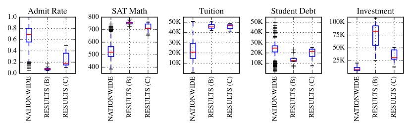
Figure 3: Combining predictive relevance probability in the Bayesian Query Language (BQL) with standard techniques in SQL to search the US College Scorecard dataset. The full data contains over 7000 colleges and 1700 variables, and is available for download at collegescorecard.ed.gov/data.

2 Establishing an information theoretic definition of context-specific predictive relevance

[width=]figures/relevance-mi-hypotheses-same

(a) Same generative process for $\mathbf{x}_{\mathcal{Q}}$ and $x_{r}$.

[width=]figures/relevance-mi-hypotheses-diff

(b) Different generative processes for $\mathbf{x}_{\mathcal{Q}}$ and $x_{r}$.

Figure 4: The predictive relevance of a collection of query records $\mathcal{Q}$ to a candidate record $r$, in the context of variable $c$, computes the probability that $\mathbf{x}_{[\mathcal{Q},c]}$ and $x_{[r,c]}$ are drawn from 4(a) the same generative process, versus 4(b) different generative processes. The latent variables $z_{0}$ and $z_{1}$ are indicators for the generative process of the records; and $\theta^{c}_{0}$ (resp. $\theta^{c}_{1})$ are distributional parameters of data under model $z_{0}$ (resp. $z_{1}$) for variable $c$. Hyperparameter $\alpha$ dictates the prior on $z$, and $\lambda$ dictates the prior on distributional parameters $\theta$. The symbol $c^{*}$ denotes a new dimension which is statistically dependent on $c$, and for which no values are observed for either $\mathcal{Q}$ or $r.$ Conditioned on hyperparameters, knowing $X_{[r,c^{*}]}$ in 4(a) carries information about the unknown values $\mathbf{X}_{[\mathcal{Q},c^{*}]}$, whereas in 4(b) it does not.

⬇

%bql SELECT "country", "oil", "hdi"

... FROM population

... WHERE "government" IS NOT 'monarchy'

... ORDER BY

... RELEVANCE PROBABILITY

... TO HYPOTHETICAL ROW WITH VALUES

... (("oil"=27, "snow"=0.2, "hdi"=180))

... IN THE CONTEXT OF "hdi"

Query Results

country	oil	hdi
USA	31	197
Australia	19
Greece	03	180
Peru	17	147
China	21
Lebanon		145
…	…	…

CrossCat-Incorporate-Record (Algorithm 3)CrossCat-Predictive-Relevance (Algorithm 1) BayesDB Query Engine

Country	Relevance Prob
	$\hat{\bm{\phi}}^{1}$	$\hat{\bm{\phi}}^{2}$	$\hat{\bm{\phi}}^{3}$	avg
China	0	1	0	0.33
USA	1	1	1	1.00
Lebanon	0	0	0	0.00
Greece	1	0	1	0.66
Australia	1	0	1	0.66
Peru	1	0	0	0.33
…	…	…	…

SQLSorting

Figure 5: BayesDB workflow for computing context-specific predictive relevance between database records. Modeling and inference in BayesDB produces an ensemble of posterior CrossCat model structures. Each structure specifies (i) a column partition for the factorization of the joint distribution of all variables in the database, using a Chinese restaraunt process; and (ii) a separate row partition within each block of variables, using a Dirichlet process mixture. The column partition clusters variables into different “contexts”, where all variables in a context are probably dependent on one another. With each context, the row partition clusters records which are probably informative of one another. End-user queries for predictive relevance are expressed in Bayesian Query Langauge. The BQL interpreter aggregates relevance probabilities across the ensemble, and can use them as a ranking function in a probabilistic ORDER BY query.

In this section, we outline the basic set-up and notations for the database search problem, and establish a formal definition of the probability of “predictive relevance” between records in the database.

2.1 Finding predictively relevant records

Suppose we are given a sparse dataset $\mathscr{D}\,{=}\,\left\{{\mathbf{x}_{1},\mathbf{x}_{2},\dots,\mathbf{x}_{N}}\right\}$ containing $N$ records, where each $\mathbf{x}_{r}\,{=}\,(x_{[r,1]},\dots,x_{[r,p]})$ is an instantiation of a $p$-dimensional random vector, possibly with missing values. For notational convenience, we refer to arbitrary collections of observations using sets as indices, so that $\mathbf{x}_{[R,C]}\,{\equiv}\,\left\{{x_{[r,c]}:r\in{R},c\in{R}}\right\}$. Bold-face symbols denote multivariate entities, and variables are capitalized as $X_{[r,c]}$ when they are unobserved (i.e. random).

Let $\mathcal{Q}\,{\subset}\,[N]$ index a small collection of “query records” $\mathbf{x}_{\mathcal{Q}}\,{=}\,\left\{{\mathbf{x}_{q}:q\in\mathcal{Q}}\right\}$. Our objective is to rank each item $\mathbf{x}_{i}\,{\in}\,\mathscr{D}$ by how relevant it is for formulating predictions about values of $\mathbf{x}_{\mathcal{Q}}$, “in the context” of a particular dimension $c$. We formally define the context of $c$ as a subset of dimensions $\mathcal{V}\,{\subseteq}\,[p]$ such that for an arbitrary record $r^{*}$ and each $v\,{\in}\,\mathcal{V}$, the random variable $X_{[r^{*},v]}$ is statistically dependent with $X_{[r^{*},c]}$.

In other words, we are searching for records $i$ where knowledge of $\mathbf{x}_{[i,\mathcal{V}]}$ is useful for predicting $\mathbf{x}_{[\mathcal{Q},\mathcal{V}]}$, had we not known the values of these observations.

2.2 Defining context-specific predictive relevance using mutual information

We now formalize the intuition from the previous section more precisely. Let $\mathcal{R}_{c}(\mathcal{Q},r)$ denote the probability that $r$ is predictively relevant to $\mathcal{Q}$, in the context of $c$. Furthermore, let $c^{*}$ denote the index of a new dimension in the length-$p$ random vectors, which is statistically dependent on dimension $c$ (i.e. is in its context) but is not one of the $p$ existing variables in the database. Since $c^{*}$ indexes a novel variable, its value for each row $r$ is itself a random variable, which we denote $X_{[r,c^{*}]}$. We now define the probability that $r$ is predictively relevant to $\mathcal{Q}$ in the context of $c$ as the posterior probability that the mutual information of $X_{[r,c^{*}]}$ and each query record $X_{[q,c^{*}]}$ is non-zero:

$$\mathcal{R}_{c}(\mathcal{Q},r)=$$ (1)

$$\quad\quad\mathbb{P}\left[\bigcap\limits_{q\in\mathcal{Q}}\left(\mathcal{I}(X_{[q,c^{*}]}:X_{[r,c^{*}]})>0\right)\mathrel{\bigg{|}}\lambda_{c^{*}},\alpha,\mathscr{D}\right].$$

The symbol $\lambda_{c^{*}}$ refers to an arbitrary set of hyperparameters which govern the distribution of dimension $c^{*}$, and $\alpha$ is a context-specific hyperparameter which controls the prior on structural dependencies between the random variables $\left\{{X_{[r,c^{*}]}:r\in[N]}\right\}$. Moreover, the mutual information $\mathcal{I}$, a well-established measure for the strength of predictive relationships between random variables (Cover and Thomas, 2012), is defined in the usual way,

$$\mathcal{I}(X_{[q,c^{*}]}:X_{[r,c^{*}]}\mid\lambda_{c^{*}},\alpha,\mathscr{D})=$$ (2)

$$\quad\mathbb{E}\left[\log\left(\frac{p(X_{[q,c^{*}]},X_{[r,c^{*}]}|\lambda_{c^{*}},\alpha,\mathscr{D})}{p(X_{[q,c^{*}]}|\lambda_{c^{*}},\alpha,\mathscr{D})p(X_{[r,c^{*}]}|\lambda_{c^{*}},\alpha,\mathscr{D})}\right)\right].$$

Figure 4 illustrates the predictive relevance probability in terms of a hypothesis test on two competing graphical models, where the mutual information is non-zero in panel 4(a) indicating predictive relevance; and zero in panel 4(b), indicating predictive irrelevance.

2.3 Related Work

Our formulation of predictive relevance in terms of mutual information between new variables $X_{[r,c^{*}]}$ is related to the idea of “property induction” from the cognitive science literature (Rips, 1975; Osherson et al., 1990; Shafto et al., 2008), where subjects are asked to predict whether an entity has a property, given that some other entity has that property; e.g. how likely are cats to have some new disease, given that mice are known to have the disease?

It is also informative to consider the relationship between the predictive relevance $\mathcal{R}_{c}(\mathcal{Q},r)$ in Eq (1) and the Bayesian Sets ranking function from the statistical modeling literature (Ghahramani and Heller, 2005):

$$\textrm{score}_{\textrm{Bayes-Sets}}(\mathcal{Q},r)=\frac{p(\mathbf{x}_{r}{\mid}\mathbf{x}_{\mathcal{Q}})}{p(\mathbf{x}_{r})}.$$ (3)

Bayes Sets defines a Bayes Factor, or ratio of marginal likelihoods, which is used for hypothesis testing without assuming a structure prior. On the other hand, predictive relevance defines a posterior probability, whose value is between 0 and 1, and therefore requires a prior over dependence structure between records (our approach outlined in Section 3 is based on nonparametric Bayes). While Bayes Sets draws inferences using only the query and candidate rows without considering the rest of the data, predictive relevance probabilities are necessarily conditioned on $\mathscr{D}$ as in Eq (1). Finally Bayes Sets considers the entire data vectors for scoring, whereas predictive relevance considers only dimensions which are in the context of a variable $c$, making it possible for two records to be predictively relevant in some context but probably predictively irrelevant in another.

3 Computing the probability of predictive relevance using nonparametric Bayes

This section describes the cross-categorization prior (CrossCat, Mansinghka et al. (2016)) and outlines algorithms which use CrossCat to efficiently estimate predictive relevance probabilities Eq (1) for sparse, high-dimensional, and heterogenously-typed data tables.

CrossCat is a nonparametric Bayesian model which learns the full joint distribution of $p$ variables using structure learning and divide-and-conquer. The generative model begins by partitioning the set of $p$ variables into blocks using a Chinese restaurant process. This step is CrossCat’s “outer” clustering, since it partitions the columns of a data table where variables correspond to columns, and records correspond to rows. Let $\pi$ denote the partition of $[p]$ whose $k$-th block is $\mathcal{V}^{k}\,{\subseteq}\,[p]$: for $j\,{\neq}\,{k}$, all variables in $\mathcal{V}^{k}$ are mutually (marginally and conditionally) independent of all variables in $\mathcal{V}^{j}$. Within block $k$, the variables $\mathbf{x}_{[r,\mathcal{V}^{k}]}$ follow a Dirichlet process mixture model (Escobar and West, 1995), where we focus on the case the joint distribution factorizes given the latent cluster assignment $z^{k}_{r}$. This step is an “inner” clustering in CrossCat, since it specifies a cluster assignment for each row in block $k$. CrossCat’s combinatorial structure requires detailed notation to track the latent variables and dependencies between them. The generative process for an exchangeable sequence $(\mathbf{X}_{1},\dots,\mathbf{X}_{N})$ of $N$ random vectors is summarized below.

Table 3: Symbols used to describe CrossCat prior

Symbol	Description
$\alpha_{0}$	Concentration hyperparameter of column CRP
$\alpha_{1}$	Concentration hyperparameter of row CRP
$v_{c}$	Index of variable $c$ in column partition
$\mathcal{V}^{k}$	List of variables in block $k$ of column partition
$z^{k}_{r}$	Cluster index of $r$ in row partition of block $k$
$\mathcal{C}^{k}_{y}$	List of rows in cluster $y$ of block $k$
$M_{c}$	Joint distribution of data for variable $c$
$\lambda_{c}$	Hyperparameters of $M_{c}$
$X_{[r,c]}$	$r$-th observation of variable $c$
$\textsc{Set}(l)$	Unique items in list $l$

CrossCat Prior 1. Sample column partition into blocks. $\mathbf{v}=(v_{1},\dots,v_{p})\sim\textsc{Crp}(\cdot|\alpha_{0})$ $\mathcal{V}^{k}\leftarrow\left\{{c\,{\in}\,[p]:v_{c}\,{=}\,k}\right\}$ foreach $k\,{\in}\,\textsc{Set}(\mathbf{v})$ 2. Sample row partitions within each block. $\mathbf{z}^{k}\,{=}\,(z^{k}_{1},\dots,z^{k}_{N})\sim\textsc{Crp}(\cdot|\alpha_{1})$ foreach $k\,{\in}\,\textsc{Set}(\mathbf{v})$ $\mathcal{C}^{k}_{y}\leftarrow\left\{{r\,{\in}\,[N]:z^{k}_{r}\,{=}\,y}\right\}$ foreach $k\,{\in}\,\textsc{Set}(\mathbf{v})$ foreach $y\,{\in}\,\textsc{Set}(\mathbf{z}^{k})$ 3. Sample data jointly within row cluster. $\left\{{X_{[r,c]}:r\in\mathcal{C}^{k}_{y}}\right\}\sim M_{c}(\cdot|\lambda_{c})$ foreach $k\,{\in}\,\textsc{Set}(\mathbf{v})$ foreach $y\,{\in}\,\textsc{Set}(\mathbf{z}^{k})$ foreach $c\,{\in}\,\mathcal{V}^{k}$

The representation of CrossCat in this paper assumes that data within a cluster is sampled jointly (step 3), marginalizing over cluster-specific distributional parameters:

$$M_{c}(\mathbf{x}_{[\mathcal{C}^{k}_{y},c]},\lambda_{c})=\int_{\theta}\prod_{r\in{\mathcal{C}^{k}_{y}}}p(x_{[r,c]}|\theta)p(\theta|\lambda_{c})d\theta.$$

This assumption suffices for our development of predictive relevance, and is applicable to a broad class of statistical data types (Saad and Mansinghka, 2016) with conjugate prior-likelihood representations such as Beta-Bernoulli for binary, Dirichlet-Multinomial for categorical, Normal-Inverse-Gamma-Normal for real values, and Gamma-Poisson for counts.

Given dataset $\mathscr{D}$, we refer to Obermeyer et al. (2014) and Mansinghka et al. (2016) for scalable algorithms for posterior inference in CrossCat, and assume we have access to an ensemble of $H$ posterior samples $\left\{{\hat{\bm{\phi}}^{1},\dots,\hat{\bm{\phi}}^{H}}\right\}$ where each $\hat{\bm{\phi}}^{h}$ is a realization of all variables in Table 3.

3.1 Estimating predictive relevance using CrossCat

We now describe how to use posterior samples of CrossCat to efficiently estimate the predictive relevance probability $\mathcal{R}_{c}(\mathcal{Q},r)$ from Eq (1). Letting $c$ denote the context variable, we formalize the novel variable $c^{*}$ as a fresh column in the tabular population which is assigned to the same block $k$ as $c$ (i.e. $k\,{=}\,v_{c}\,{=}\,v_{c^{*}})$. As shown by Saad and Mansinghka (2017), structural dependencies induced by CrossCat’s variable partition are related to an upper-bound on the probability there exists a statistical dependence between $c$ and $c^{*}$. To estimate Eq (1), we first treat the mutual information between $X_{[q,c^{*}]}$ and $X_{[r,c^{*}]}$ as a derived random variable, which is a function of their random cluster assignments $z^{k}_{q}$ and $z^{k}_{r}$,

$$(z^{k}_{q},z^{k}_{r})\mapsto\mathcal{I}(X_{[q,c^{*}]}:X_{[r,c^{*}]}|z^{k}_{q},z^{k}_{r},\alpha_{1},\lambda_{c^{*}}).$$ (4)

The key insight, implied by step 3 of the CrossCat prior, is that, conditioned on their assignments, rows from different clusters are sampled independently, which gives

$$z^{k}_{q}\neq z^{k}_{r}$$

$${\iff}\,p(x_{[q,c^{*}]},x_{[r,c^{*}]}|z^{k}_{q},z^{k}_{r},\lambda_{c^{*}},\alpha_{1},\mathscr{D})=$$

$$\quad\quad p(x_{[q,c^{*}]}|z^{k}_{q},\lambda_{c^{*}},\alpha_{1},\mathscr{D})p(x_{[r,c^{*}]}|z^{k}_{r},\lambda_{c^{*}},\alpha_{1},\mathscr{D})$$

$${\iff}\,\mathcal{I}(X_{[q,c^{*}]}:X_{[r,c^{*}]}|z^{k}_{q},z^{k}_{r},\alpha_{1},\lambda_{c^{*}})=0,$$ (5)

where the final implication follows directly from the definition of mutual information in Eq (2). Note that Eq (5) does not depend on the particular choice of $\lambda_{c^{*}}$, and indeed this hyperparameter is never represented explicitly. Moreover, hyperparameter $\alpha_{1}$ (corresponding to $\alpha$ in Figure 4) is the concentration of the Dirichlet process for CrossCat row partitions.

Eq (5) implies that we can estimate the probability of non- zero mutual information between $X_{[r,c^{*}]}$ and each $X_{[q,c^{*}]}$ for $q\,{\in}\,\mathcal{Q}$ by forming a Monte Carlo estimate from the ensemble of posterior CrossCat samples,

$$\mathcal{R}_{c}(\mathcal{Q},r)$$

$$=\mathbb{P}\left[\bigcap\limits_{q\in\mathcal{Q}}\left(\mathcal{I}(X_{[q,c^{*}]}:X_{[r,c^{*}]})>0\right)\mathrel{\bigg{|}}\lambda_{c^{*}},\alpha_{1},\mathscr{D}\right]$$

$$=\mathbb{P}\left[\bigcap\limits_{q\in\mathcal{Q}}\left(z^{v_{c}}_{q}=z^{v_{c}}_{r}\right)\mathrel{\bigg{|}}\alpha_{1},\mathscr{D}\right]$$

$$\approx\frac{1}{H}\sum_{h=1}^{H}\left[\mathbb{I}\left[\bigcap\limits_{q\in\mathcal{Q}}\left(\hat{z}^{\hat{v}_{c}^{h},h}_{q}=\hat{z}^{\hat{v}_{c}^{h},h}_{r}\right)\right]\right],$$ (6)

where $\hat{v}_{c}^{h}$ indexes the context block, and $\hat{z}^{\hat{v}_{c}^{h},h}_{r}$ denotes cluster assignment of $r$ in the row partition of $\hat{v}_{c}^{h}$, according to the sample $\hat{\bm{\phi}}^{h}$. Algorithm 1 outlines a procedure (used by the BayesDB query engine from Figure 5) for formulating a Monte Carlo based estimator for a predictive relevance query using CrossCat.

Algorithm 1 CrossCat-Predictive-Relevance

1:$\left\{\begin{array}[]{l}\mbox{CrossCat samples:}\;\hat{\bm{\phi}}^{h}\;\mbox{for}\;h=1{,}\dots,H\\ \mbox{query rows:}\;\mathcal{Q}=\left\{{{q_{i}}:1\leq{i}\leq\lvert\mathcal{Q}\rvert}\right\}\\ \mbox{context variable:}\;c\\ \end{array}\right.$

2:predictive relevance of each existing row in $\mathscr{D}$ to $\mathcal{Q}$ 

3:for $r=1,\dots,N$ do $\triangleright$ for each existing row

4:  for $h=1,\dots,H$ do $\triangleright$ for each CrossCat sample

5:   $k\leftarrow\hat{v}^{h}_{c}$ $\triangleright$ retrieve the context block

6:   for $q\in\mathcal{Q}$ do $\triangleright$ for each query row

7:     if $\hat{z}^{k,h}_{q}\neq\hat{z}^{k,h}_{r}$ then $\triangleright$ $r$ and $q$ are different clusters

8:      $\mathcal{R}^{h}_{c}(\mathcal{Q},r)\leftarrow 0$ $\triangleright$ $r$ irrelevant to some $q$

9:      break         

10:   else$\triangleright$ $r$ in same cluster as all $q\in\mathcal{Q}$

11:     $\mathcal{R}^{h}_{c}(\mathcal{Q},r)\leftarrow 1$ $\triangleright$ $r$ relevant to all $q$      

12:  $\mathcal{R}_{c}(\mathcal{Q},r)\leftarrow\frac{1}{H}\sum_{h=1}^{H}\mathcal{R}^{h}_{c}(\mathcal{Q},r)$ $\triangleright$ average relevances

13:return $\left\{{\mathcal{R}_{c}(\mathcal{Q},r):1\leq{r}\leq{N}}\right\}$

3.2 Optimizing the estimator using a sparse matrix-vector multiplication

In this section, we show how to greatly optimize the naive, nested for-loop implementation in Algorithm 1 by instead computing predictive relevance for all $r$ through a single matrix-vector multiplication.

Define the pairwise cluster co-occurrence matrix $\mathbf{S}^{k,h}$ for block $k$ of CrossCat sample $\hat{\bm{\phi}}^{h}$ to have binary entries $\mathbf{S}^{k,h}_{i,j}\,{=}\,\mathbb{I}[\hat{z}^{k,h}_{i}\,{=}\,\hat{z}^{k,h}_{j}]$. Furthermore, let $\mathbf{1}_{\mathcal{Q}}$ denote a length-$N$ vector with a 1 at indexes $q\,{\in}\,\mathcal{Q}$ and 0 otherwise. We vectorize $\mathcal{R}_{c}(\mathcal{Q},r)$ across $r\,{\in}\,[N]$ by:

$$\mathbf{u}^{h} =\frac{1}{\lvert\mathcal{Q}\rvert}\;\mathbf{S}^{k,h}\;\mathbf{1}_{\mathcal{Q}} h=1,\dots,H$$ (7)

$$\mathcal{R}_{c}(\mathcal{Q},\cdot) =\frac{1}{H}\sum_{h=1}^{H}\mathbf{u}^{h}.$$ (8)

The resulting length-$N$ vector $\mathbf{u}^{h}$ in Eq (7) satisfies $\mathbf{u}^{h}_{r}\,{=}\,1$ if and only if $\hat{z}^{k,h}_{r}\,{=}\,\hat{z}^{k,h}_{q}$ for all $q\,{\in}\,\mathcal{Q}$, which we identify as the argument of the indicator function in Eq (6). Finally, by averaging $\mathbf{u}^{h}$ across the $H$ samples in Eq (8), we arrive at the vector of relevance probabilities.

For large datasets, constructing the $N{\times}{N}$ matrix $\mathbf{S}^{k,h}$ using $\Theta(N^{2})$ operations is prohibitively expensive. Algorithm 2 describes an efficient procedure that exploits CrossCat’s sparsity to build $\mathbf{S}^{k,h}$ in expected time ${\ll}\,O(N^{2})$ by using (i) a sparse matrix representation, and (ii) CrossCat’s partition data structures to avoid considering all pairs of rows. This fast construction means that Eq (7) is practical to implement for large data tables.

The algorithm’s running time depends on (i) the number of clusters $\lvert\textsc{Set}(\hat{\mathbf{z}}^{k})\rvert$ in line 3; (ii) the average number of rows per cluster $\lvert\hat{\mathcal{C}}^{k}_{y}\rvert$ in line 4; and (iii) the data structures used to represent $\mathbf{S}^{k,h}$ in line 5. Under the CRP prior, the expected number of clusters is $O(\alpha_{1}\log(N))$, which implies an average occupancy of $O(N/(\alpha_{1}\log(N)))$ rows per cluster. If the sparse binary matrix is stored with a list-of-lists representation, then the update in line 5 requires $O(1)$ time. Furthermore, we emphasize that since $\mathbf{S}^{k,h}$ does not depend $\mathcal{Q}$, its cost of construction is amortized over an arbitrary number of queries.

Algorithm 2 CrossCat-Co-Occurrence-Matrix

1:CrossCat sample $\hat{\bm{\phi}}^{h}$; block index $k$.

2:Pairwise co-occurrence matrix $\mathbf{S}^{k,h}$

3:for $y\in\textsc{Set}(\hat{\mathbf{z}}^{k})$ do $\triangleright$ for each cluster in block $k$

4:  for $r\in\hat{\mathcal{C}}^{k}_{y}$ do $\triangleright$ for each row in the cluster

5:   Set $\mathbf{S}^{k,h}_{r,j}=1$, where $j\in\hat{\mathcal{C}}^{k}_{y}$ $\triangleright$ update the matrix   

6:return $\mathbf{S}^{k,h}$

3.3 Computing predictive relevance probabilities for query records that are not in the database

We have so far assumed that the query records must consist of items that already exist in the database. This section relaxes this restrictive assumption by illustrating how to compute relevance probabilities for search records which do not exist in $\mathscr{D}$, and are instead specified by the user on a per-query basis (refer to the BQL query in Figure 5 for an example of a hypothetical query record). The key idea is to (i) incorporate the new records into each CrossCat sample $\hat{\bm{\phi}}^{h}$ by using a Gibbs-step to sample cluster assignments from the joint posterior (Neal, 2000); (ii) compute Eq (7) on the updated samples; and (iii) unincorporate the records, leaving the original samples unmutated.

Letting $\left\{{\mathbf{x}_{[N+i]}:1\leq{i}\leq{t}}\right\}$ denote $t$ (partially observed) new rows and $\mathcal{Q}=\left\{{N{+}1,\dots,N{+}t}\right\}$ the query, we compute $\mathcal{R}_{c}(\mathcal{Q},r)$ for all $r$ by first applying CrossCat-Incorporate-Record (Algorithm 3) to each $q\,{\in}\,\mathcal{Q}$ sequentially. Sequential incorporation corresponds to sampling from the sequence of predictive distributions, which, by exchangeability, ensures that each updated $\hat{\bm{\phi}}^{h}$ contains a sample of cluster assignments from the joint distribution, guaranteeing correctness of the Monte Carlo estimator in Eq (6). Note that since CrossCat specifies a non-parametric mixture, the proposal clusters include all existing clusters, plus one singleton cluster $\max(\mathbf{z}^{k})\,{+}\,1$. We next update the co-occurrence matrices in time linear in the size of the sampled cluster and then evaluate Eq (7) and (8). To unincorporate, we reverse lines 9-11 and restore the co-occurrence matrices. Figure 6 confirms that the runtime scaling is asymptotically linear, varying the (i) number of new rows, (ii) fraction of variables specified for the new rows that are in the context block (i.e. query sparsity), (iii) number of clusters in the context block, and (iv) number of variables in the context block.

Algorithm 3 CrossCat-Incorporate-Record

1:CrossCat sample $\bm{\phi}$; context $c$; new row $\mathbf{x}_{N+1}$

2:Updated crosscat sample $\bm{\phi}^{\prime}$

3:$k\leftarrow v_{c}$ $\triangleright$ Retrieve block of context variable

4:$Y\leftarrow\max(\mathbf{z}^{k})+1$ $\triangleright$ Retrieve proposal clusters

5:for $y\,{=}\,1,\dots,Y$ do $\triangleright$ Compute cluster probabilities

6:     $n_{y}\leftarrow\begin{cases}\left|{\mathcal{C}^{k}_{y}}\right|&\text{if }y\in\mathbf{z}^{k}\\ \alpha_{1}&\text{if }y=\max({\mathbf{z}^{k}})\,{+}\,1\end{cases}$

7:     $l_{y}\leftarrow\left(\prod_{c\in\mathcal{V}^{k}}M_{c}(x_{[N{+}1,c]}|\mathbf{x}_{[\mathcal{C}^{k}_{y},c]},\lambda_{c})\right)n_{y}$

8:$z^{k}_{N+1}\sim\textsc{Categorical}(l_{1},\dots,l_{Y})$ $\triangleright$ Sample cluster

9:${\mathbf{z}^{\prime}}^{k}\leftarrow\mathbf{z}^{k}\cup\left\{{z^{k}_{N+1}}\right\}$ $\triangleright$ Append cluster assignment

10:${\mathcal{C}^{\prime}}^{k}_{z^{k}_{N{+}1}}\leftarrow\mathcal{C}^{k}_{z^{k}_{N+1}}\cup\left\{{N{+}1}\right\}$ $\triangleright$ Append row to cluster

11:$\mathscr{D}^{\prime}\leftarrow\mathscr{D}\cup\left\{{\mathbf{x}_{[N+1,\mathcal{V}^{k}]}}\right\}$ $\triangleright$ Append record to database

12:return $\bm{\phi}^{\prime}$ $\triangleright$ Return the updated sample

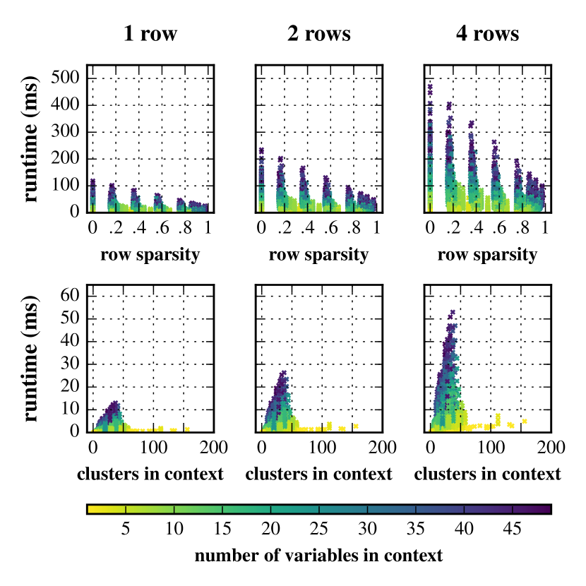
Figure 6: Empirical measurements of the asymptotic scaling of CrossCat-Incorporate-Record (Algorithm 3) on the Gapminder dataset (Section 4). The color of each measurement indicates the number of variables in the block of the context variable; each column shows a different number of records (1, 2, 4, and 8) incorporated by the algorithm. The top panels shows that, for a fixed number of variables in the context, the runtime (in milliseconds) decays linearly with the sparsity of the hypothetical records (dimensions which are not in the same block as the context variable are ignored). The lower panels show the runtime increasing linearly with the number of clusters in the context; the number of variables in the context dictates the slope of the curve.

(a) Pairwise CrossCat predictive relevances in different contexts

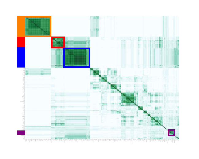
(b) CrossCat (life expectancy)

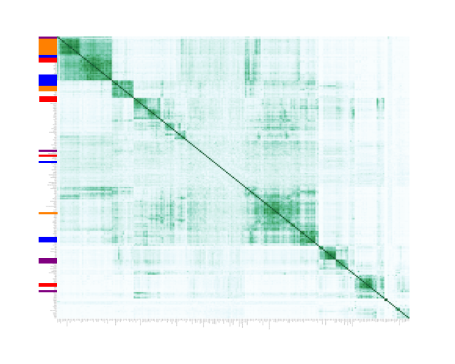
(c) CrossCat (exports, % gdp)

(d) Pairwise cosine similarities in different contexts

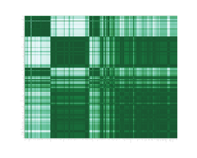
(e) Cosine (life expectancy)

(f) Cosine (exports, % gdp)

Concept	Representative Countries in the Concept
Low-Income Nations	Burundi, Ethiopia, Uganda, Benin, Malawi, Rwanda, Togo, Guinea, Senegal, Afghanistan, Malawi
Post-Soviet Nations	Russia, Ukraine, Bulgaria, Belarus, Slovakia, Serbia, Croatia, Poland, Hungary, Romania, Latvia
Western Democracies	France, Britain, Germany, Netherlands, Italy, Denmark, Finland, Sweden, Norway, Australia, Japan
Small Wealthy Nations	Qatar, Bahrain, Kuwait, Emirates, Singapore, Israel, Gibraltar, Bermuda, Jersey, Cayman Islands

(a) Countries which are mutually predictive in the context of “life expectancy” according to CrossCat’s relevance matrix 7(b).

Figure 7: 7(b) – 7(f) Pairwise heatmaps of countries from the Gapminder dataset in the contexts of “life expectancy at birth” and “exports of goods and services (% of gdp) ”, using CrossCat predictive relevance and cosine similarity. Each row and column in a matrix is a country, and a cell value (between 0 and 1) indicates the strength of match between those two countries. 4(a) CrossCat learns a sparse set of relevances; for “life expectancy”, these broadly correspond to common-sense taxonomies of countries based on shared geographic, political and macroeconomic characteristics. These concepts were manually labeled by inspecting clusters of countries in matrix 7(b); the colors in the matrix correspond to countries in the table which belong to the concept of that color. Note that the relevance structure differs significantly when ranking in the context of “exports, % gdp”, as shown by the colors in matrix 7(c) where the clusters of mutually relevant countries form a different pattern than in 7(b). Cosine similarity learns dense, noisy sets of spuriously high-ranking countries with coarser structure, as shown in 7(e) and 7(f). Refer to Appendix C for more baselines.

⬇

%bql .barplot

... ESTIMATE "country",

... RELEVANCE PROBABILITY

... TO EXISTING ROWS IN

... ('United States')

... IN THE CONTEXT OF

... "life expectancy at birth"

... AS "rel_us_lifexp"

... FROM gapminder

... ORDER BY "rel_us_lifexp" DESC

... LIMIT 15

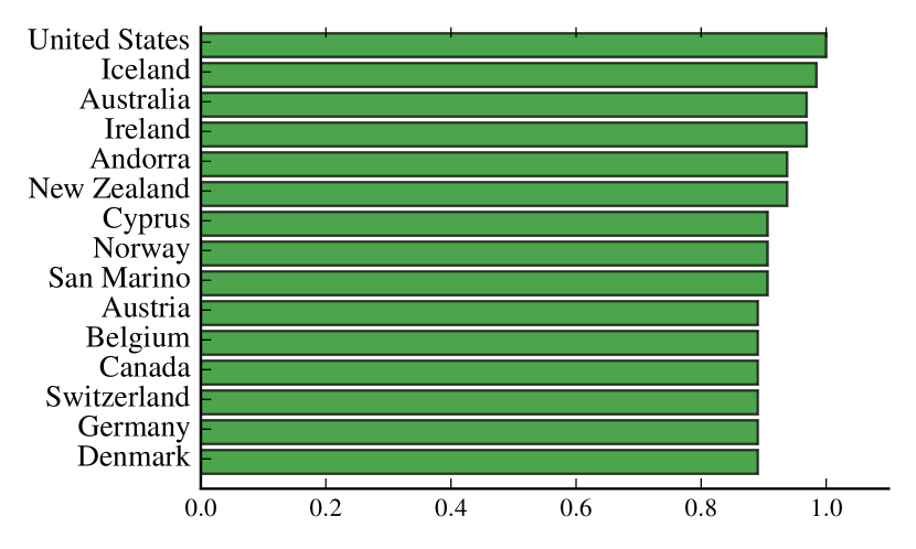
(a) Relevance to USA in the context of “life expectancy”

Measles, mumps, & rubella vaccines (% population)

Under 5 mortality rate

Dead children per woman

access to improved sanitation facilities (% population)

access to improved drinking water sources (% population)

human development index

body mass index (kg/m2)

murder rate (per 100,000)

food supply (kilocalories per person)

contraceptive prevalence (% women ages 15-49)

alcohol consumption (liters per adult)

prevalence of tobacco use among adults (% population)

(a) Variables in the context of “life expectancy at birth”

Figure 8: Using BQL to search for the top 15 countries in the Gapminder dataset ranked by their relevance to the United States in the context of “life expectancy at birth” finds rich, Western democracies with advanced healthcare systems.

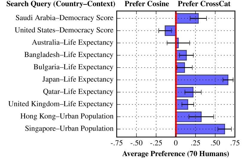
Figure 9: Comparing human preferences for the top-ranked countries returned by cosine similarity versus CrossCat predictive relevance, in 10 representative search queries (shown on the y-axis). For each query, human subjects were given the top 10 most relevant countries, according to both cosine and CrossCat, and then asked to choose which results they preferred, if any. We scored the responses in the following way: “countries returned by cosine are more relevant” (score = -1); “countries returned by CrossCat are more relevant” (score = +1); “both results are equally relevant” (score = 0). The x-axis shows the scores averaged across 70 humans, surveyed on the cloud through crowdflower.com. Error bars represent one standard error of the mean. For most of the queries, human preferences are biased in favor of CrossCat’s rankings. Further details on the experimental design and results are given in Appendix B.

4 Applications

This section illustrates the efficacy of predictive relevance in BayesDB by applying the technique to several search problems in real-world, sparse, and high-dimensional datasets of public interest.

4.1 College Scorecard

The College Scorecard (Council of Economic Advisers, 2015) is a federal dataset consisting of over 7000 colleges and 1700 variables, and is used to measure and improve the performance of US institutions of higher education. These variables include a broad set of categories such as the campus characteristics, academic programs, student debt, tuition fees, admission rates, instructional investments, ethnic distributions, and completion rates. We analyzed a subset of 2000 schools (four-year institutions) and 100 variables from the categories listed above.

Suppose a student is interested in attending a city university with a set of desired specifications. Starting with a standard SQL Boolean search in Figure 1(a) (on p. 3) they find only one matching record, which requires iteratively rewriting the search conditions to retrieve more results.

Figure 2(a) instead expresses the search query as a hypothetical row in a BQL PREDICTIVE RELEVANCE query (which invokes the technique in Section 3.3). The top-ranking records contain first-rate schools, but their admission rates are much too stringent. In Figure 3(a), the user re-expresses the BQL query to rank schools by predictive relevance, in the context of instructional investment, to a subset of the first-rate schools discovered in 2(a). Combining ORDER BY PREDICTIVE RELEVANCE with Boolean conditions in the WHERE clause returns another set of top-quality schools with city-campuses that are less competitive than those in 2(a), but have quantitative metrics that are much better than national averages.

4.2 Gapminder

Gapminder (Rosling, 2008) is an extensive longitudinal dataset of over $\sim$320 global macroeconomic variables of population growth, education, climate, trade, welfare and health for 225 countries. Our experiments are based on a cross-section of the data from the year 2002. The data is sparse, with 35% of the data missing. Figure 7 shows heatmaps of the pairwise predictive relevances for all countries in the dataset under different contexts, and compares the results to cosine similarity. Clusters of predictively relevant countries form common-sense taxonomies; refer to the caption for further discussion.

Figure 8 finds the top-15 countries in the dataset ordered by their predictive relevance to the United States, in the context of “life expectancy at birth”. Table 5(a) shows representative variables which are in the context; these variables have the highest dependence probability with the context variable, according a Monte Carlo estimate using 64 posterior CrossCat samples. The countries in Figure 8(a) are all rich, Western democracies with highly developed economies and advanced healthcare systems.

To quantitatively evaluate the quality of top-ranked countries returned by predictive relevance, we ran the technique on 10 representative search queries (varying the country and context variable) and obtained the top 10 results for each query. Figure 9 shows the queries, and human preferences for the results from predictive relevance versus results from cosine similarity between the country vectors. We defined the context for cosine similarity by the 320-dimensional vectors down to 10 dimensions and selecting variables which are most dependent with the context variable according to CrossCat’s dependence probabilities. To deal with sparsity, which cosine similarity cannot handle natively, we imputed missing values using sample medians; imputation techniques like MICE (Buuren and Groothuis-Oudshoorn, 2011) resulted in little difference (Appendix C).

5 Discussion

This paper has shown how to perform probabilistic searches of structured data by combining ideas from probabilistic programming, information theory, and nonparametric Bayes. The demonstrations suggest the technique can be effective on sparse, real-world databases from multiple domains and produce results that human evaluators often preferred to a standard baseline.

More empirical evaluation is clearly needed, ideally including tests of hundreds or thousands of queries, more complex query types, and comparisons with query results manually provided by human domain experts. In fact, search via predictive relevance in the context of variables drawn from learned representations of data could potentially provide a meaningful way to compare representation learning techniques. It also may be fruitful to build a distributed implementation suitable for database representations of web-scale data, including photos, social network users, and web pages.

Relatively unstructured probabilistic models, such as topic models, proved sufficient for making unstructured text data far more accessible and useful. We hope this paper helps illustrate the potential for structured probabilistic models to improve the accessibility and usefulness of structured data.

Acknowledgments

The authors wish to acknowledge Ryan Rifkin, Anna Comerford, Marie Huber, and Richard Tibbetts for helpful comments on early drafts. This research was supported by DARPA (PPAML program, contract number FA8750-14-2-0004), IARPA (under research contract 2015-15061000003), the Office of Naval Research (under research contract N000141310333), the Army Research Office (under agreement number W911NF-13-1-0212), and gifts from Analog Devices and Google.

Appendix A Integrating predictive relevance as a ranking function in BayesDB

This section describes the integration of predictive relevance into BayesDB (Mansinghka et al., 2015; Saad and Mansinghka, 2016), a probabilistic programming platform for probabilistic data analysis.

New syntaxes in the Bayesian Query Language (BQL) allow a user to express predictive relevance queries where the query set can be an arbitrary combination of existing and hypothetical records. We implement predictive relevance in BQL as an expression with the following syntaxes, depending on the specification of the query records.

• Query records are existing rows.

  ⬇

  RELEVANCE PROBABILITY

  TO EXISTING ROWS IN <expression>

  IN THE CONTEXT OF <context-var>

• Query records are hypothetical rows.

  ⬇

  RELEVANCE PROBABILITY

  TO HYPOTHETICAL ROWS WITH VALUES (<values>)

  IN THE CONTEXT OF <context-var>

• Query records are existing and hypothetical rows.

  ⬇

  RELEVANCE PROBABILITY

  TO EXISTING ROWS IN <expression>

  AND HYPOTHETICAL ROWS WITH VALUES (<values>)

  IN THE CONTEXT OF <context-var>

The expression is formally implemented as a 1-row BQL estimand, which specifies a map $r\mapsto\mathcal{R}_{c}(\mathcal{Q},r)$ for each record in the table. As shown in the expressions above, query records are specified by the user in two ways: (i) by giving a collection of EXISTING ROWS, whose primary key indexes are either specified manually, or retrieved using an arbitrary BQL <expression>; (ii) by specifying one or more HYPOTHETICAL RECORDS with their <values> as a list of column-value pairs. These new rows are first incorporated using Algorithm 3 from Section 3.3 and they are then unincorporated after the query is finished. The <context-var> can be any variable in the tabular population.

As a 1-row function in the structured query language, the RELEVANCE PROBABILITY expression can be used in a variety of settings. Some typical use-cases are shown in the following examples, where we use only existing query rows for simplicity.

• As a column in an ESTIMATE query.

  ⬇

  ESTIMATE

  "rowid",

  RELEVANCE PROBABILITY

  TO EXISTING ROWS IN <expression>

  IN THE CONTEXT OF <context-var>

  FROM <table>

• As a filter in WHERE clause.

  ⬇

  ESTIMATE

  "rowid"

  FROM <table>

  WHERE (

  RELEVANCE PROBABILITY

  TO EXISTING ROWS IN <expression>

  IN THE CONTEXT OF <context-var>

  ) > 0.5

• As a comparator in an ORDER BY clause.

  ⬇

  ESTIMATE

  "rowid"

  FROM <table>

  ORDER BY

  RELEVANCE PROBABILITY

  TO EXISTING ROWS IN <expression>

  IN THE CONTEXT OF <context-var>

  [ASC | DESC]

It is also possible to perform arithmetic operations and Boolean comparisons on relevance probabilities.

• Finding the mean relevance probability for a set of rowids of interest.

  ⬇

  ESTIMATE

  AVG (

  RELEVANCE PROBABILITY

  TO EXISTING ROWS IN <expression>

  IN THE CONTEXT OF <context-var>

  )

  FROM <table>

  WHERE "rowid" IN <expression>

• Finding rows which are more relevant in some context $c_{0}$ than in another context $c_{1}$.

  ⬇

  ESTIMATE

  "rowid"

  FROM <table>

  WHERE (

  RELEVANCE PROBABILITY

  TO EXISTING ROWS IN <expression>

  IN THE CONTEXT OF <context-var-0>

  ) > (

  RELEVANCE PROBABILITY

  TO EXISTING ROWS IN <expression>

  IN THE CONTEXT OF <context-var-1>

  )

Appendix B Predictive relevance and cosine similarity on Gapminder human evaluation queries

(a) Saudi Arabia, Democracy

A
Saudi
Oman
Libya
Kuwait
W. Sahara
Qatar
Bahrain
Algeria
Iraq
Emirates
Bhutan

B
Saudi
Venezuela
Israel
Trdad & Tob
Malta
Puerto Rico
Oman
Spain
Canada
Japan
Argentina

(b) United States, Democracy

A
USA
France
Finland
Norway
UK
Sweden
Estonia
Denmark
Australia
Switzerland
Germany

B
USA
Australia
Ireland
Canada
UK
Iceland
Netherlands
Austria
Denmark
Japan
New Zealand

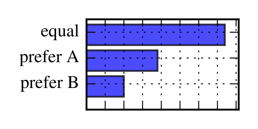
(c) Australia, Life Expectancy

A
Australia
Ireland
Iceland
Andorra
United States
New Zealand
Austria
Belgium
Canada
Switzerland
Cyprus

B
Australia
Israel
Germany
Canada
Iceland
Malta
Ireland
Finland
United States
Luxembourg
UK

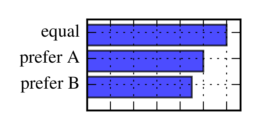
(d) Bangladesh, Life Expectancy

A
Bangladesh
Bhutan
Papua NG
India
Gambia
Uganda
Nepal
Timor-Leste
Pakistan
Mauritania
Indonesia

B
Bangladesh
India
Bhutan
Myanmar
Indonesia
Philippines
Nepal
Pakistan
Mongolia
Viet Nam
Kyrgyzstan

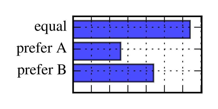
(e) Bulgaria, Life Expectancy

A
Bulgaria
Estonia
Portugal
Macedonia
Kuwait
Bosnia
Hungary
Croatia
Spain
Japan
Poland

B
Bulgaria
Croatia
Poland
Serbia
Hungary
Slovakia
Bosnia
Belarus
Montenegro
Estonia
Montserrat

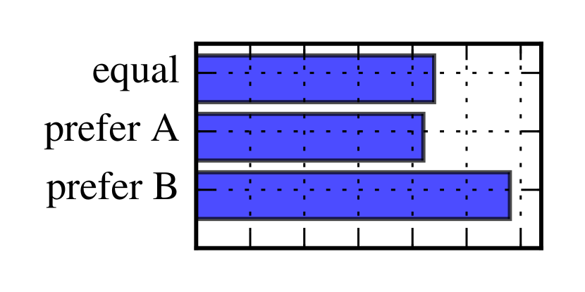
(f) Japan, Life Expectancy

A
Japan
Hungary
Portugal
Spain
Slovakia
Greece
Kuwait
Slovenia
Emirates
Poland
Ireland

B
Japan
Austria
Belgium
Canada
Switzerland
Germany
Denmark
Finland
France
UK
Netherlands

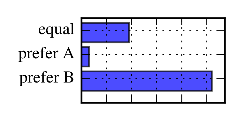
(g) Qatar, Life Expectancy

A
Qatar
Emirates
Kuwait
Bahrain
Turks Isld
Cayman Isld
Guernsey
Bermuda
Jersey
Israel
Singapore

B
Qatar
Serbia
Bosnia
Belarus
Croatia
Montenegro
Estonia
Bulgaria
Lithuania
Latvia
Saudi Arabia

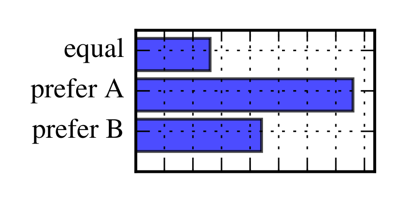
(h) UK, Life Expectancy

A
UK
Belgium
France
Luxembourg
Slovenia
Germany
Malta
Canada
Finland
Ireland
Czechia

B
UK
Austria
Belgium
Canada
Switzerland
Germany
Denmark
Finland
France
Japan
Netherlands

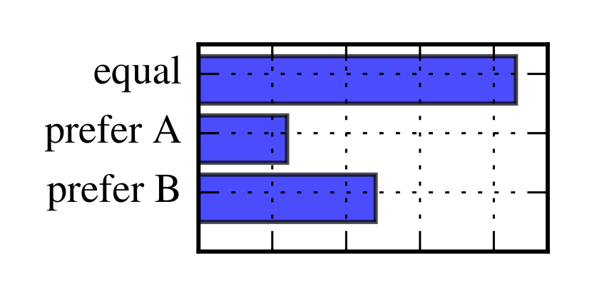
(i) Hong Kong, Urban Pop

A
Hong Kong
Italy
Mexico
Finland
Bulgaria
Belgium
Lithuania
Slovakia
Poland
Lebanon
Panama

B
Hong Kong
Singapore
Austria
Canada
Greenland
Netherlands
Andorra
Switzerland
Ireland
Iceland
Denmark

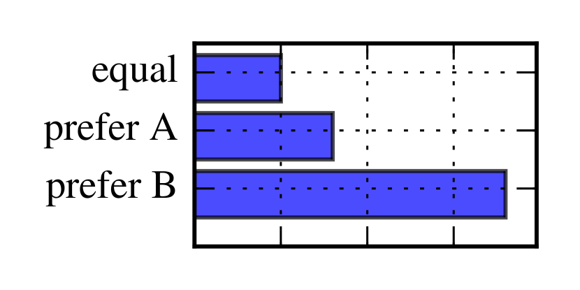
(j) Singapore, Urban Pop

A
Singapore
Barbados
Oman
Norway
Romania
Libya
Algeria
Palau
Gabon
Cuba
Switzerland

B
Singapore
Hong Kong
Gibraltar
Andorra
Monaco
United States
San Marino
Luxembourg
Norway
Austria
Australia

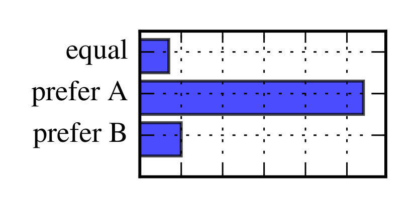
Figure 10: The top-10 ranking countries returned by predictive relevance and cosine similarity for each of the 10 queries used for the human evaluation in Figure 9. For each country-context search query, we showed seventy subjects (surveyed on the AI crowdsourcing platform %****␣cosine.tex␣Line␣425␣****crowdflower.com) a pair of tables. We then asked each subject to select the table which contains more relevant results to the search query, or report that both tables contain equally relevant results. The tables above show the top-ranked countries using CrossCat predictive relevance and cosine similarity, with a histogram of the human responses. The caption of Figure 9 describes how we converted these raw histograms into scores between -1 and 1 that are displayed in the main text. The tables showing countries ranked using CrossCat predictive relevance are: Saudi Arabia (A); United States (B); Australia (A); Bangladesh (B); Bulgaria (B); Japan (B); Qatar (A); UK (B); Hong Kong (B); Singapore (B).

Appendix C Pairwise heatmaps on Gapminder countries using baseline methods

(a) Cosine Similarity

(b) Median Imputation (5 vars)

(c) Median Imputation (10 vars)

(d) Median Imputation (15 vars)

(e) Median Imputation (20 vars)

(f) MICE Imputation (5 vars)

(g) MICE Imputation (10 vars)

(h) MICE Imputation (15 vars)

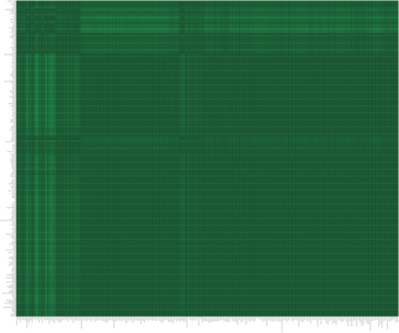
(i) MICE Imputation (20 vars)

(j) Bray-Curtis Coefficent

(k) Median Imputation (5 vars)

(l) Median Imputation (10 vars)

(m) Median Imputation (15 vars)

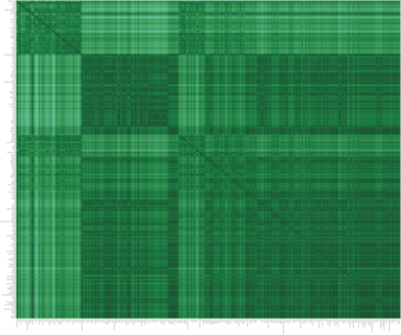
(n) Median Imputation (20 vars)

(o) MICE Imputation (5 vars)

(p) MICE Imputation (10 vars)

(q) MICE Imputation (15 vars)

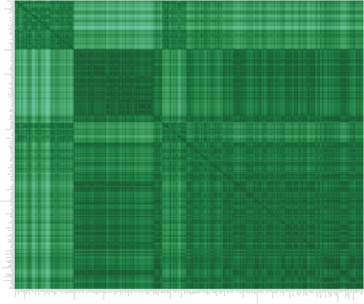
(r) MICE Imputation (20 vars)

(s) Euclidean Distance

(t) Median Imputation (5 vars)

(u) Median Imputation (10 vars)

(v) Median Imputation (15 vars)

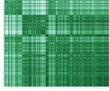
(w) Median Imputation (20 vars)

(x) MICE Imputation (5 vars)

(y) MICE Imputation (10 vars)

(z) MICE Imputation (15 vars)

(aa) MICE Imputation (20 vars)

Figure 11: Pairwise heatmaps of countries in Gapminder dataset in the context of “life expectancy at birth”, using various distance and similarity measures on the country vectors. Each heatmap is labeled with the imputation technique (median or MICE (Buuren and Groothuis-Oudshoorn, 2011)), and the number of variables in the context (i.e. dimensionality of the vectors). These techniques struggle with sparsity and their structures are much noisier than the results of relevance probability shown in Figure 7(b) and Table 4(a).

Appendix D Application to a dataset of 1987 cars

⬇

%bql CREATE TABLE cars_1987_raw

... FROM 'cars_1987.csv'

%bql SELECT

... "make",

... "price",

... "wheels",

... "doors",

... "engine",

... "horsepower",

... "body"

... FROM cars_1987_raw

... WHERE "price" < 45000

... AND "wheels" = 'rear'

... AND "doors" = 'four

... AND "engine" >= 250

... AND "horsepower" > 180

... AND "body" sedan

(a) Suppose a customer wishes to purchase a classic car from 1987 with a budget of $45,000 and a desired set of technical specifications. They first load a csv file of 200 cars with 26 variables into a BayesDB table, and then specify the search conditions as Boolean filters in a SQL WHERE clause. Due to sparsity in the table, only one record is returned. To obtain more relevant results, the user needs to broaden the specifications in the query.

make	price	wheels	doors	engine	horsepower	body
mercedes	40,960	rear	four	308	184	sedan

⬇

%mml CREATE POPULATION

... cars_1987

... FOR cars_1987_raw

... WITH SCHEMA (

... GUESS STATISTICAL

... TYPES FOR (*);

... )

%mml CREATE METAMODEL m FOR cars_1987

... WITH BASELINE crosscat;

%mml INITIALIZE 100 MODELS FOR m;

%mml ANALYZE m FOR 1 MINUTE;

%bql .heatmap ESTIMATE

... DEPENDENCE PROBABILITY

... FROM PAIRWISE VARIABLES

... OF cars_1987

%bql SELECT

... "make",

... "price",

... "wheels",

... "doors",

... "engine-size",

... "horsepower",

... "style"

... FROM cars_1987

... ORDER BY

... RELEVANCE PROBABILITY

... TO HYPOTHETICAL ROW ((

... "price" = 42000,

... "wheels" = 'rear',

... "doors" = 'four',

... "engine" = 250,

... "horsepower" = 180,

... "body" = 'sedan'

... ))

... IN THE CONTEXT OF

... "price"

... LIMIT 10

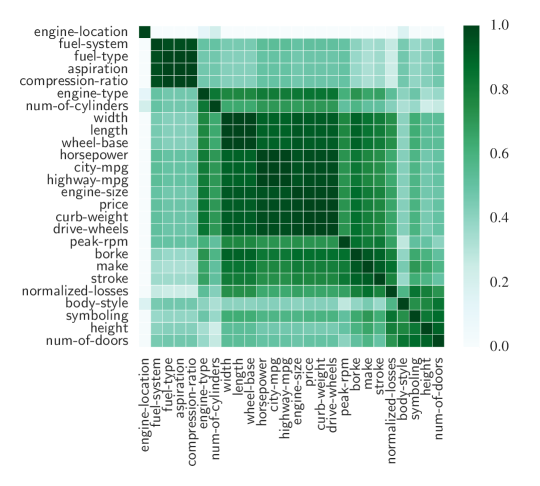
(a) Building CrosssCat models in BayesDB for the cars_1987 population learns a full joint probabilistic model over all variables. The ESTIMATE DEPENDENCE PROBABILITY query allows the user to plot a heatmap of probable dependencies between car characteristics. The context of ‘‘price’’ probably contains the majority of other variables in the search query.

(b) Using ORDER BY RELEVANCE PROBABILITY in BQL ranks each car in the table by its relevance to the user’s specifications, which are specified as a hypothetical row. The top-10 ranked cars by probability of relevance to the search query, in the context of price, are shown below in the table below. The user can now inspect further characteristics of this subset of cars, to find ones that they like best.

make	price	wheels	doors	engine	horsepower	body
jaguar	35,550	rear	four	258	176	sedan
jaguar	32,250	rear	four	258	176	sedan
mercedes	40,960	rear	four	308	184	sedan
mercedes	45,400	rear	two	304	184	hardtop
mercedes	34,184	rear	four	234	155	sedan
mercedes	35,056	rear	two	234	155	convertible
bmw	36,880	rear	four	209	182	sedan
bmw	41,315	rear	two	209	182	sedan
bmw	30,760	rear	four	209	182	sedan
jaguar	36,000	rear	two	326	262	sedan

Figure 13: A session in BayesDB for probabilistic model building and search in the cars dataset (Kibler et al., 1989).

References

- Buuren and Groothuis-Oudshoorn (2011) Stef Buuren and Karin Groothuis-Oudshoorn. mice: Multivariate imputation by chained equations in r. Journal of Statistical Software, 45(3), 2011.
- Council of Economic Advisers (2015) Council of Economic Advisers. Using federal data to measure and improve the performance of u.s. institutions of higher education. Technical report, Executive Office of the President of the United States, 2015.
- Cover and Thomas (2012) Thomas Cover and Joy Thomas. Elements of Information Theory. Wiley Series in Telecommunications and Signal Processing. Wiley, 2012.
- Escobar and West (1995) Michael Escobar and Mike West. Bayesian density estimation and inference using mixtures. Journal of the American Statistical Association, 90(430):577–588, 1995.
- Ghahramani and Heller (2005) Zoubin Ghahramani and Katherine A. Heller. Bayesian sets. In Proceedings of the 18th International Conference on Neural Information Processing Systems, pages 435–442. MIT Press, 2005.
- Kibler et al. (1989) Dennis Kibler, David W Aha, and Marc K Albert. Instance-based prediction of real-valued attributes. Computational Intelligence, 5(2):51–57, 1989.
- Mansinghka et al. (2015) Vikash Mansinghka, Richard Tibbetts, Jay Baxter, Pat Shafto, and Baxter Eaves. BayesDB: A probabilistic programming system for querying the probable implications of data. CoRR, abs/1512.05006, 2015.
- Mansinghka et al. (2016) Vikash Mansinghka, Patrick Shafto, Eric Jonas, Cap Petschulat, Max Gasner, and Joshua B. Tenenbaum. CrossCat: A fully Bayesian nonparametric method for analyzing heterogeneous, high dimensional data. Journal of Machine Learning Research, 17(138):1–49, 2016.
- Neal (2000) Radford M Neal. Markov chain sampling methods for dirichlet process mixture models. Journal of Computational and Graphical Statistics, 9(2):249–265, 2000.
- Obermeyer et al. (2014) Fritz Obermeyer, Jonathan Glidden, and Eric Jonas. Scaling nonparametric Bayesian inference via subsample-annealing. In Proceedings of the Seventeenth International Conference on Artificial Intelligence and Statistics, pages 696–705. JMLR.org, 2014.
- Osherson et al. (1990) Daniel N Osherson, Edward E Smith, Ormond Wilkie, Alejandro Lopez, and Eldar Shafir. Category-based induction. Psychological review, 97(2):185, 1990.
- Rips (1975) Lance J. Rips. Inductive judgments about natural categories. Journal of Verbal Learning and Verbal Behavior, 14(6):665–681, 1975.
- Rosling (2008) Hans Rosling. Gapminder: Unveiling the beauty of statistics for a fact based world view, 2008. URL https://www.gapminder.org/data/.
- Saad and Mansinghka (2016) Feras Saad and Vikash Mansinghka. Probabilistic data analysis with probabilistic programming. CoRR, abs/1608.05347, 2016.
- Saad and Mansinghka (2017) Feras Saad and Vikash Mansinghka. Detecting dependencies in sparse, multivariate databases using probabilistic programming and non-parametric bayes. In Proceedings of the Twentieth International Conference on Artificial Intelligence and Statistics. JMLR.org, 2017.
- Shafto et al. (2008) Patrick Shafto, Charles Kemp, Elizabeth Bonawitz, John Coley, and Joshua Tenenbaum. Inductive reasoning about causally transmitted properties. Cognition, 109(2):175–192, 2008.