Reweighting from the mixture distribution as a better way to describe the Multistate Bennett Acceptance Ratio

Abstract

The multistate Bennett Acceptance ratio is provably the lowest variance unbiased estimator of both free energies and ensemble averages, and has a number of important advantages over previous methods, such as WHAM. Despite its advantages, the original MBAR paper was rather dense and mathematically complicated, limiting the extent to which people could expand and apply it. We present here a different way to think about MBAR that is much more intuitive and makes it clearer why the method works so well.

I Introduction

Several years ago, we derived the multistate Bennett Acceptance ratio (MBAR) Shirts and Chodera (2008), an approach to compute free energies and expectation averages computed from samples from multiple thermodynamics states. Based on results in statistical inference, Vardi (1985); Gill et al. (1988); Kong et al. (2003); Tan (2004), this method is provably the lowest variance unbiased estimators of both free energies and ensemble averages. Additionally, it has a number of important advantages over previous methods. Multiple histogram techniques, such as WHAM, rely on histograms of width sufficient to contain many samples, which introduces a bias that can be substantial and often difficult to assess Kobrak (2003). Additionally, using multiple histogram techniques makes it very difficult to compute error estimates in the free energies or ensemble averages obtained. MBAR uses no histograms, estimating quantities using the samples directly, and thus has no histogram bias. It is important to note that equation for free energies itself was derived by Souaille and Roux in 2001 Souaille and Roux (2001) as the limit of WHAM as bins go to zero width, so the equation itself was not new, but the context, connection to statistics, proofs of minimum variance, and useful formula for uncertainties in the free energies and observables were novel.

MBAR reduces exactly to Bennett’s acceptance ratio formula in the case of only two states Bennett (1976), motivating our original name. BAR, therefore, does have provably lowest variance for the free energy calculation between two states, suffers no histogram bias, and has a robust variance estimate. However, it cannot be used to directly compute free energies using samples for multiple states all together (only in pairs), and cannot be used to compute ensemble averages in its standard formulation. MBAR, as we showed in our original paper, follows the same general mathematical derivation as BAR, yielding provably lowest variance free energies as well as robust variance estimates, but extended to multiple states, and the mathematical framework allows computing the expectation values of observables as well.

Despite all these advantages, the original MBAR paper was rather dense and mathematically complicated, somewhat suppressing the understanding of the approach and therefore, its use by other researchers for practical problems. We present here a different way to think about MBAR that is hopefully much more intuitive and makes it clearer why it works well.

II Original mathematical definition of MBAR

First, some definitions. Suppose we obtain $N_{i}$ uncorrelated equilibrium samples MLE from each of $K$ thermodynamics states within the same class of ensemble (such as all NVT, all NPT, all ${\bf\mu}$VT, etc.). Each state is characterized by a specified combination of inverse temperature, potential energy function, pressure, and/or chemical potential(s), depending upon the ensemble. We define the reduced potential function $u_{i}({\mbox{\boldmath{$x$}}})$ for state $i$ to be

$$u_{i}({\mbox{\boldmath{$x$}}}) = \beta_{i}[U_{i}({\mbox{\boldmath{$x$}}})+p_{i}V({\mbox{\boldmath{$x$}}})+{\mbox{\boldmath{$\mu$}}}_{i}^{\mathrm{T}}{\mbox{\boldmath{$n$}}}({\mbox{\boldmath{$x$}}})]$$ (1)

where ${\mbox{\boldmath{$x$}}}\in{\bf\Gamma}$ denotes the configuration of the system within a configuration space ${\bf\Gamma}$, with volume $V({\mbox{\boldmath{$x$}}})$ (in the case of a constant pressure ensemble) and ${\mbox{\boldmath{$n$}}}({\mbox{\boldmath{$x$}}})$ the number of molecules of each of $M$ components of the system (in the case of a grand or semigrand ensemble). For each state $i$, $\beta_{i}$ is the inverse temperature, $U_{i}({\mbox{\boldmath{$x$}}})$ the potential energy function (which may include biasing weights), $p_{i}$ the external pressure, and ${\mbox{\boldmath{$\mu$}}}_{i}$ the vector of chemical potentials of the $M$ system components. This formalism allows a very large number of different situations to be described by the same mathematics.

In all of these situations, configurations $\{{\mbox{\boldmath{$x$}}}_{in}\}_{n=1}^{N_{i}}$ from state $i$ are sampled from the probability distribution

$$p_{i}({\mbox{\boldmath{$x$}}})=c_{i}^{-1}q_{i}({\mbox{\boldmath{$x$}}})\> \>c_{i}=\int_{{\bf\Gamma}}d{\mbox{\boldmath{$x$}}}\,q_{i}({\mbox{\boldmath{$x$}}})$$ ; (2)

where $q_{i}({\mbox{\boldmath{$x$}}})$ is here nonnegative and represents an unnormalized density function. $c_{i}$ is the (generally unknown) normalization constant (which of course, in statistical mechanics is simply the partition function). In samples obtained from standard Metropolis Monte Carlo or molecular dynamics simulations or from experiment, this unnormalized density $q_{i}({\mbox{\boldmath{$x$}}})$ is simply the Boltzmann weight $\exp[-u_{i}({\mbox{\boldmath{$x$}}})]$ but the general math allows it to be an arbitrary probability distribution, such as found in simulations employing non-Boltzmann weights, such as multicanonical simulations Mezei. (1987) or Tsallis statistics Tsallis (1988).

What we want is an efficient and simple estimator for the difference in dimensionless free energies

$$\Delta f_{ij} \equiv f_{j}-f_{i}=-\ln\frac{c_{j}}{c_{i}}=-\ln\frac{\int_{\bf\Gamma}d{\mbox{\boldmath{$x$}}}\,q_{j}({\mbox{\boldmath{$x$}}})}{\int_{\bf\Gamma}d{\mbox{\boldmath{$x$}}}\,q_{i}({\mbox{\boldmath{$x$}}})}$$ (3)

where the $f_{i}$ are related to the dimensionalized free energies $F_{i}$ by $f_{i}=\beta_{i}F_{i}$.

We would also like to have useful estimators of the equilibrium expectations of some observable (energy, volume, pair distances, etc.) of the coordinates $O({\mbox{\boldmath{$x$}}})$.

$$\left\langle O\right\rangle_{i} \equiv \int_{{\bf\Gamma}}d{\mbox{\boldmath{$x$}}}\,p_{i}({\mbox{\boldmath{$x$}}})\,O({\mbox{\boldmath{$x$}}})=\frac{\int_{\bf\Gamma}d{\mbox{\boldmath{$x$}}}\,O({\mbox{\boldmath{$x$}}})\,q_{i}({\mbox{\boldmath{$x$}}})}{\int_{\bf\Gamma}d{\mbox{\boldmath{$x$}}}\,q_{i}({\mbox{\boldmath{$x$}}})}.$$ (4)

The original MBAR paper Shirts and Chodera (2008) presented a way to estimate these ratios of normalization constants through the identity

$$c_{i}\left\langle\alpha_{ij}q_{j}\right\rangle_{i}=\int_{{\bf\Gamma}}d{\mbox{\boldmath{$x$}}}\,q_{i}({\mbox{\boldmath{$x$}}})\,\alpha_{ij}({\mbox{\boldmath{$x$}}})\,q_{j}({\mbox{\boldmath{$x$}}})=c_{j}\left\langle\alpha_{ij}q_{i}\right\rangle_{j}$$ (5)

which holds for arbitrary choice of functions $\alpha_{ij}({\mbox{\boldmath{$x$}}})$, provided the $c_{i}$ are nonzero. It is possible to construct the $\alpha_{ij}(x)$ which leads to minimum variance in the free energies, and obtain a self-consistent nonlinear equation for the $c_{i}$ that has a unique solution, up to a multiplicative constant:

$$\hat{c}_{i}=\sum_{n=1}^{N}\frac{q_{i}({\mbox{\boldmath{$x$}}}_{n})}{\sum\limits_{k=1}^{K}N_{k}\,\hat{c}_{k}^{-1}\,\ q_{k}({\mbox{\boldmath{$x$}}}_{n})},$$ (6)

where $N=\sum_{k=1}^{K}N_{k}$. One can also construct an estimate of the asymptotic error of the estimate of $c_{i}(x)$. (Shirts and Chodera, 2008)

In terms of free energies, this becomes.

$$\hat{f}_{i} = -\ln\sum_{j=1}^{K}\sum_{n=1}^{N_{j}}\frac{\exp[-u_{i}({\mbox{\boldmath{$x$}}}_{jn})]}{\sum\limits_{k=1}^{K}N_{k}\,\exp[\hat{f}_{k}-u_{k}({\mbox{\boldmath{$x$}}}_{jn})]}$$ (7)

Again, because the normalization constants are only determined up to a multiplicative constant, the estimated free energies $\hat{f}_{i}$ are determined uniquely only up to an additive constant, so only differences $\Delta\hat{f}_{ij}=\hat{f}_{j}-\hat{f}_{i}$ will be meaningful. Estimators of the uncertainties in $\Delta\hat{f}_{ij}$ can again be derived and are given in a previous paper Shirts and Chodera (2008).

For a free energy $f_{i}$ of a state from which no samples are collected, then we can use the same equation, but we note that the denominator does not contain that potential, so the free energy does not require any self-consistent iteration, but instead only requires running through once, using precomputed denominators.

Once one has computed the normalizing constants (and therefore the free energies), then one can estimate the equilibrium expectation of any observable $O({\mbox{\boldmath{$x$}}})$ that depends only on configuration $x$ is given by Eq. 4. This expectation can be computed as a ratio of “normalization” constants $c_{O}/c_{a}$ by defining the additional function

$$q_{O}({\mbox{\boldmath{$x$}}})=O({\mbox{\boldmath{$x$}}})\,q({\mbox{\boldmath{$x$}}})$$ (8)

While $q_{O}({\mbox{\boldmath{$x$}}})$ may no longer be strictly nonnegative, we may still make use of the equation as long as it does not appear in the denominator dos , which is the case, since we are not calculating from this distribution. It’s robust and works well, but is a bit convoluted. But as we see, there are simpler ways to think about these expectations (more on that in a bit).

We can write this ratio of integrals as:

$$\langle O_{i}\rangle=\sum_{n}O_{i}(x_{n})W_{in}$$ (9)

where:

$$W_{ni}=\hat{c}_{i}^{-1}\,q_{i}({\mbox{\boldmath{$x$}}}_{n})/\sum\limits_{k=1}^{K}N_{k}\,\hat{c}_{k}^{-1}\,\ q_{k}({\mbox{\boldmath{$x$}}}_{n}).$$ (10)

Or, for the Boltzmann distribution:

$$W_{ni}=\frac{\exp[\hat{f}_{i}-u_{i}({\mbox{\boldmath{$x$}}}_{n})]}{\sum\limits_{k=1}^{K}N_{k}\,\exp[\hat{f}_{k}-u_{k}({\mbox{\boldmath{$x$}}}_{n})]}$$ (11)

Note that we are now indexing the weights by a single index $n=1,\ldots,N$, rather than a separate index for each state, as, surprisingly, the association of which samples ${\mbox{\boldmath{$x$}}}_{n}$ came from which distribution $p_{i}({\mbox{\boldmath{$x$}}})$ does not enter into the calculation! We could literally forget which state each sample came from, and get the same answers. Why is this?

III MBAR as importance sampling from the mixture distribution

A much simpler way to interpret MBAR which provides significant insight is as reweighting from a mixture distribution. To describe this well, we first need to review the idea of importance sampling.

One can calculate averages of any observable $O(\vec{x})$ with respect to a normalized probability distribution $p_{i}(\vec{x})$ by integrating over the support of that distribution.

$$\langle O\rangle_{i}=\int_{\Gamma}O(\vec{x})p_{i}(\vec{x})d\vec{x}$$

Where the subscript $i$ indicates that the average is with respect to the distribution $p_{i}(\vec{x})$, and $\Gamma$ is the phase space volume we integrate over. If we pick samples $\vec{x}$ proportional to their probability $p_{i}(\vec{x})$, then we can calculate the same averages by Monte Carlo integration.

$$\langle O\rangle_{i}=\frac{1}{N}\sum_{n=1}^{N}O(\vec{x}_{n})$$

where $N$ is the number of samples collected.

We can divide and multiply by $p_{j}(\vec{x})$ to find that:

$$\langle O\rangle_{i}=\int_{\Gamma}O(\vec{x})\left(\frac{p_{i}(\vec{x})}{p_{j}(\vec{x})}\right)p_{j}(\vec{x})d\vec{x}$$

Given a well-behaved $p_{j}(\vec{x})$, if we can generate samples from the normalized distribution $p_{j}(\vec{x})$, then we have:

$$\langle O\rangle_{i}=\frac{1}{N}\sum_{n=1}^{N}O(\vec{x}_{n})\left(\frac{p_{i}(\vec{x}_{n})}{p_{j}(\vec{x}_{n})}\right)$$

This equation gives us expectations in state $i$, but with samples from state $j$.

Note that to do this, we assumed that $p_{j}(\vec{x})$ is nonzero in any finite volume of interest in $p_{i}(\vec{x})$. In most cases, this will not be relevant, because if $p_{j}(\vec{x})=0$, we will not collect samples from it anyway, so it doesn’t matter that the ratio is undefined, and because with standard pair potentials (Coulomb’s law, Lennard-Jones, etc.), $p_{j}(\vec{x})=0$ is only true at single points with zero total volume. There are some complications with hard spheres with changing radii, but we will not explore the issues there at this time.

If $p_{j}(\vec{x})$ is almost zero where $p_{i}(\vec{x})$ has substantial probability density, then the integrals will eventually converge, but it will take a very large number of samples. An example of this latter case is in the insertion of a Lennard-Jones sphere in a dense fluid, with $p_{j}(\vec{x})$ the distribution with a zero potential and $p_{i}(\vec{x})$ is the distribution with the Lennard-Jones potential present. Only with configurations with other fluid particles at the exact center of the Lennard-Jones sphere is $p_{j}(\vec{x})=0$, but it is very nearly zero for a substantial number of configurations with fluid particles near the center of the sphere, resulting in an insertion is very inefficient. A number of alternative techniques have been developed (such as soft core approaches and staged insertion) to improve the convergence of integrals in this situation.

If we know our distributions $p_{i}(\vec{x})$ and $p_{j}(\vec{x})$ only up to unknown constants $c_{i}$ and $c_{j}$, so that $p_{i}(\vec{x})=c_{i}^{-1}q_{i}(\vec{x})$, then it seems we are stuck; how can we deal with the unknown ratio $c_{i}/c_{j}$? We can introduce a trick; we choose for the observable $O(\vec{x})=1$, which yields (for samples collected from the unnormalized distribution $q_{i}(\vec{x})$):

$$\langle 1\rangle_{i} = \frac{1}{N}\sum_{n=1}^{N}\left(1\right)\frac{c_{j}}{c_{i}}\left(\frac{q_{i}(\vec{x}_{n})}{q_{j}(\vec{x}_{n})}\right)$$

$$1 = \frac{1}{N}\sum_{n=1}^{N}\frac{c_{j}}{c_{i}}\left(\frac{q_{i}(\vec{x}_{n})}{q_{j}(\vec{x}_{n})}\right)$$

$$\frac{c_{i}}{c_{j}} = \frac{1}{N}\sum_{n=1}^{N}\left(\frac{q_{i}(\vec{x}_{n})}{q_{j}(\vec{x}_{n})}\right)$$ (12)

since the expectation of 1 is always 1, and 1=1 no matter what state we are in. In the case of Boltzmann-form distributions, then $c_{i}=e^{-f_{i}}$, the generalized free energy, and $q_{i}(\vec{x})=e^{-u_{i}(\vec{x})}$, which reduces to

$$f_{j}-f_{i} = -\ln\frac{1}{N}\sum_{n=1}^{N}e^{-(u_{i}(\vec{x}_{n})-u_{j}(\vec{x}_{n}))}$$ (13)

$$= -\ln\left\langle e^{-(u_{i}(\vec{x})-u_{j}(\vec{x}))}\right\rangle_{j}$$

where $\langle\rangle_{j}$ indicates ensemble average over the sampled distribution $j$, which is of course the standard one-state reweighting method for free energy calculations first introduced by Zwanzig.

Now, here’s the key step. Assume we have collected $N_{k}$ samples from each of $K$ different distributions $p_{k}(\vec{x})=c_{k}^{-1}q_{k}(\vec{x})$. We construct a new probability distribution where we simply throw all $N=\sum_{i=1}^{K}N_{k}$ into the same pot. The probability of drawing a sample from this mixture of distributions is going to be simply

$$p_{m}(\vec{x})=\frac{1}{N}\sum_{k=1}^{K}N_{k}p_{k}(\vec{x})$$ (14)

because there is a $\frac{N_{k}}{N}$ chance of getting a sample from each of the $K$ distributions. Once we have a sample from that distribution, the probability distribution is just $p_{k}(\vec{x})$, as we have seen.

We call this entire set of samples, together, a mixture distribution, since it involves mixing together samples from all $K$ distributions. If each of the individual $p_{k}(\vec{x})$ distributions is normalized, then it is easy to verify that the overall mixture distribution $p_{m}(\vec{x})$ must also normalized.

A visual example

Let’s look at a visual example of how one constructs this mixture distribution (Fig. 1). Let’s say we have a one-dimensional degree of freedom, and we collect an equal amount of data from a series of distributions $p_{K}$ that span this degree of freedom. We gather data from all five distributions (Fig. 1a), and pool them together (Fig. 1b) into our mixture distribution. If there are an uneven number of samples from each distribution, we simply weight each distribution by the number of samples from that distribution (Fig. 1c).

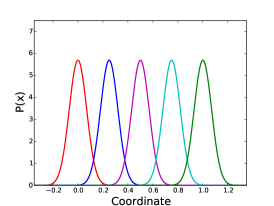
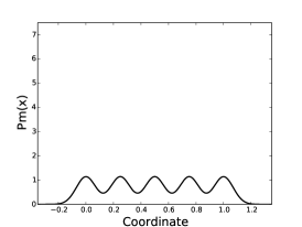
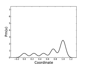
a	b	c

Figure 1: (a) Five normalized probability distributions, that together span the entire coordinate range of interest. (b) a mixture distribution $p_{m}(x)$ with even number of samples of each of five distributions. (c) a mixture distribution $p_{m}(x)$ with distribution of samples with ratio 1:1:1:2:4. The mixture distributions have nonnegligible sampling across the entire configuration range of interest, meaning that we can easily reweight to samples at any of these configurations. All distributions are normalized.

How do we calculate the normalizing constants $c_{i}$ and free energies $f_{i}$ so we can reweight observables? Assume again that we only know our distributions $p_{i}(\vec{x})$ up to an unknown normalizing constant $c_{i}$. The mixture distribution can then be expressed by:

$$p_{m}(\vec{x})=\frac{1}{N}\sum N_{k}c_{k}^{-1}q_{k}(\vec{x})$$

If each of the individual distributions is normalized (i.e. we solve for $c_{k}$), then clearly the mixture distribution $p_{m}(\vec{x})$ must be normalized. If we reweight from the mixture distribution to distribution $i$, defined by $p_{i}(\vec{x})$ and use the observable $O(\vec{x})=1$ again, then we have:

$$1 = \frac{1}{N}\sum_{n=1}^{N}\frac{1}{c_{i}}\left(\frac{q_{i}(\vec{x})}{p_{m}(\vec{x})}\right)$$

$$= \frac{1}{N}\sum_{n=1}^{N}\frac{c_{i}^{-1}q_{i}(\vec{x})}{N^{-1}\sum_{k}N_{k}c_{k}^{-1}q_{k}(\vec{x_{n}})}$$

$$= \sum_{n=1}^{N}\frac{c_{i}^{-1}q_{i}(\vec{x}_{n})}{\sum_{k}N_{k}c_{k}^{-1}q_{k}(\vec{x}_{n})}$$

$$c_{i} = \sum_{n=1}^{N}\frac{q_{i}(\vec{x}_{n})}{\sum_{k}N_{k}c_{k}^{-1}q_{k}(\vec{x}_{n})}$$ (15)

Where the last equation is simply an algebraic relationship. There will be $K$ equations, one for each of the $K$ distributions. We then have a system of $K$ equations that can be solved for the $c_{k}$. Although there are $K$ equations, there are only $K-1$ independent equations. This can be seen by noting that the equations are equivalent if all $c_{k}$ are multiplied by the same constant, so we must set one number (often $c_{1}$, though it could be any of them) to some value (usually 1). In terms of the Boltzmann distribution, this becomes.

$$e^{-f_{i}} = \sum_{n=1}^{N}\frac{e^{-u_{i}(\vec{x}_{n})}}{\sum_{k}N_{k}e^{f_{k}-u_{k}(\vec{x}_{n})}}$$

Which is exactly the same as the MBAR equations for $f_{i}$ previously published.

We can also write this system of equations as:

$$1=\sum_{n=1}^{N}W_{in}$$

where:

$$W_{in}=\frac{c_{i}^{-1}q_{i}(\vec{x}_{n})}{\sum_{k}N_{k}c_{k}^{-1}q_{k}(\vec{x}_{n})}$$

which is true for each $i$, but more simply can be seen as:

$$W_{in}=\frac{1}{N}\frac{p_{i}(\vec{x}_{n})}{p_{m}(\vec{x}_{n})}$$ (16)

And is simply an expression of the fact that the weights for any of the ensemble must be normalized.

We can then calculate reweighted expectations of observables at any state from the mixture distribution, which can be written in a number of ways

$$\langle O\rangle_{i} = \frac{1}{N}\sum_{i=1}^{N}O(\vec{x}_{n})\frac{p_{i}(\vec{x}_{n})}{p_{m}(\vec{x}_{n})}$$ (17)

$$= \sum_{n=1}^{N}O(\vec{x}_{n})\frac{c_{i}^{-1}q_{i}(\vec{x}_{n})}{\sum N_{k}c_{k}^{-1}q_{k}(\vec{x}_{n})}$$

$$= \sum_{n=1}^{N}O(\vec{x}_{n})\frac{e^{f_{i}-u_{i}(\vec{x}_{n})}}{\sum N_{k}e^{f_{k}-u_{k}(\vec{x}_{n})}}$$

$$= \sum_{n=1}^{N}O(\vec{x}_{n})W_{in}$$

which can be seen as reweighting (or importance sampling) to state $i$ from the mixture distribution $p_{m}(\vec{x})$ This, again, is exactly the same equation as the previously published MBAR estimator for observables.

It then becomes clear why we don’t need to know which state each sample is from. If we are reweighting from the mixture distribution, we throw out all the information from which state each sample comes from; the calculation only cares about whether the normalized probability for each individual sample is known.

The idea of reweighting from a mixture distribution is not original to us; Geyer appears to be the first to introduced this idea in 1994 in the case of the mixture of two distributions (Geyer, 1994) in a technical report which did not really appear in published journal or conference literature; this may explain why the idea never caught hold, especially outside of the statistics community.

Hopefully, this discussion helps demystify the MBAR equations for free energy, helps make it clearer where they come from, and what they mean.

Acknowledgments

Thanks for Ye Mei (East China Normal University), Tommy Foley (Penn State), and Yuanyuan Zhou (University of Michigan) for noting typos in previous versions of this document.

References

- Shirts and Chodera (2008) M. R. Shirts and J. D. Chodera, J. Chem. Phys. 129, 124105 (2008).
- Vardi (1985) Y. Vardi, Ann. Stat. 13, 178 (1985).
- Gill et al. (1988) R. D. Gill, Y. Vardi, and J. A. Wellner, Ann. Stat. 16, 1069 (1988).
- Kong et al. (2003) A. Kong, P. McCullagh, X.-L. Meng, D. Nicolae, and Z. Tan, J. Royal Stat. Soc. B. 65, 585 (2003).
- Tan (2004) Z. Tan, J. Am. Stat. Assoc. 99, 1027 (2004).
- Kobrak (2003) M. N. Kobrak, J. Comput. Chem. 24, 1437 (2003).
- Souaille and Roux (2001) M. Souaille and B. Roux, Comp. Phys. Commun. 135, 40 (2001).
- Bennett (1976) C. H. Bennett, J. Comp. Phys. 22, 245 (1976).
- (9) A set of uncorrelated configurations can be obtained from a correlated time series, such as is generated by a molecular dynamics or Metropolis Monte Carlo simulation, by subsampling the timeseries with an interval larger than the statistical inefficiency of the reduced potential of the timeseries. The statistical inefficiency can be estimated by standard procedures Swope et al. (1982); Flyvbjerg and Petersen (1989); Janke (2002); Chodera et al. (2007).
- Mezei. (1987) E. Mezei., J. Comp. Phys. 68, 237 (1987).
- Tsallis (1988) C. Tsallis, J. Stat. Phys. 52, 479 (1988).
- (12) Honi Doss makes this suggestion in the conference discussion of Kong et al. (2003).
- Geyer (1994) C. J. Geyer, Tech. Rep. 568, School of Statistics, University of Minnesota, Minneapolis, Minnesota (1994).
- Swope et al. (1982) W. C. Swope, H. C. Andersen, P. H. Berens, and K. R. Wilson, J. Chem. Phys. 76, 637 (1982).
- Flyvbjerg and Petersen (1989) H. Flyvbjerg and H. G. Petersen, J. Chem. Phys. 91, 461 (1989).
- Janke (2002) W. Janke, in Quantum Simulations of Complex Many-Body Systems: From Theory to Algorithms, edited by J. Grotendorst, D. Marx, and A. Murmatsu (John von Neumann Institute for Computing, Jülich, Germany, 2002), vol. 10, pp. 423–445.
- Chodera et al. (2007) J. D. Chodera, W. C. Swope, J. W. Pitera, C. Seok, and K. A. Dill, J. Chem. Theor. Comput. 3, 26 (2007).