Analysis of Device-to-Device Communications in Uplink Cellular Networks with Lognormal Fading

Abstract

In this paper, using the stochastic geometry theory, we present a framework for analyzing the performance of device-to-device (D2D) communications underlaid uplink (UL) cellular networks. In our analysis, we consider a D2D mode selection criterion based on an energy threshold for each user equipment (UE). Specifically, a UE will operate in a cellular mode, if its received signal strength from the strongest base station (BS) is large than a threshold $\beta$. Otherwise, it will operate in a D2D mode. Furthermore, we consider a generalized log-normal shadowing in our analysis. The coverage probability and the area spectral efficiency (ASE) are derived for both the cellular network and the D2D one. Through our theoretical and numerical analyses, we quantify the performance gains brought by D2D communications and provide guidelines of selecting the parameters for network operations.

I Introduction

In the last decade, there has been a sharp increase in the demand for data traffic [1]. To address such massive consumer demand for data communications, especially from the user equipments (UEs) such as smartphones and tablets, many noteworthy technologies have been proposed [2], such as small cell networks (SCNs), cognitive radio, device-to-device (D2D) communications, etc. In particular, D2D communications are usually defined as directly transferring data between mobile UEs which are in proximity. Due to the short communication distance between a D2D user pair, D2D communications hold great promise in improving network performance such as coverage, spectral efficiency, energy efficiency, and delay. Recently, D2D underlaid cellular networks have been standardized by the 3rd Generation Partnership Project (3GPP). The major challenge in the D2D enabled underlaid cellular network is the inclusion of inter-tier and intra-tier interference due to the aggressive frequency reuse, where cellular UEs and D2D UEs share the same spectrum resources. In parallel with the standardization effort, recently there has been a surge of academic studies in this area [3, 4, 5, 6].

In more detail, by using the stochastic geometry theory, Andrews, et.al conducted network performance analyses for the downlink (DL) [7] and the uplink (UL) [8] of SCNs, in which UEs and/or base stations (BSs) were assumed to be randomly deployed according to a homogeneous Poisson distribution. In [9], Peng developed an analytical framework for the D2D underlaid cellular network in the DL, where the Rician fading channel model was adopted to model the small-scale fast fading for the D2D communication links. In [3], Liu provided a unified framework to analyze the downlink outage probability in a multi-channel environment with Rayleigh fading, where D2D UEs were selected based the received signal strength from the nearest BS. In [10], Sun presented an analytical framework for evaluating the network performance in terms of load-aware coverage probability and network throughput using a dynamic TDD scheme in which mobile users in proximity can engage in D2D communications. In [11], George proposed exclusion regions to protect cellular receivers from excessive interference from active D2D transmitters. In [12], the authors derived approximate expressions for the distance distribution between two D2D peers conditioned on the core network’s knowledge of the cellular network and analyzed the performance of network-assisted D2D discovery in random spatial networks.

Although the existing work provides precious insights into resource allocation and mode selection for D2D communications, there still exists several problems:

• In some studies, only a single BS with one cellular UE and one D2D pair were considered, which did not take into account the influence from other cells.

• The mode selection scheme in the literature was not very practical, which was mostly based on the distance only and considered D2D receiver UEs as an additional tier of nodes, independent of the cellular UEs and the D2D transmitter UEs. Such tier of D2D receiver UEs without cellular capabilities appears from nowhere and is hard to justify.

• D2D communications usually coexist with the UL of cellular communications due to the relatively low inter-tier interference. Such feature has not been well treated in the literature.

• The pathloss model is not practical, e.g., LOS/NLOS transmissions have not been well studied in the context of D2D, and usually the same pathloss model was used for both the cellular and the D2D tiers.

• Shadow fading was widely ignored in the analysis, which did not reflect realistic networks.

To sum up, up to now, there is no work investigating the D2D-enabled UL cellular network with the consideration of the lognormal shadow fading. To fill in this gap of theoretical study, in this paper, we consider the D2D-enhanced network and develop a tractable framework to quantify the network performance for a D2D-enabled UL cellular network. The main contributions of this paper are summarized as follows:

• We introduce a hybrid network model, in which the random and unpredictable spatial positions of mobile users and base stations are modeled as Possion point processes. This model captures several important characteristics of a D2D-enabled UL cellular network including lognormal fading, transmit power control and orthogonal scheduling of cellular users within a cell.

• We consider a flexible D2D mode selection which is based on the maximum DL received power from the strongest base station. Such maximum DL signal strength based mode selection scheme helps to mitigate the undesirable interference from D2D transmitters.

• We present a general and analytical framework, which considers that the D2D UEs are distributed according to a non-homogenous PPP. With this approach, a unified performance analysis is conducted for underlaid D2D communications and we derive analytical results in terms of the coverage probability and the area spectral efficiency (ASE) for both cellular UEs and D2D UEs. Our results shed new light on the system design of D2D communications.

The rest of this paper is organized as follows. In Section II, we introduce the system model and assumptions used in this paper. Section III presents our main results. We provide numerical results and more discussion in Section IV and conclude our work in Section V.

II System Model

In this section, we present the system model that is used in this paper.

II-A The Path Loss Model

We consider a D2D underlaid UL cellular network, where BSs and UEs, including cellular UL UEs and D2D UEs, are assumed to be distributed on an infinite two-dimensional plane $\mathbf{\mathit{\mathtt{\mathbb{R}}}^{2}}$. We assume that the cellular BSs are spatially distributed according to a homogeneous PPP of intensity $\lambda_{b}$ , i.e., $\varPhi_{b}=\{X_{i}\}$, where $X_{i}$ denotes the spatial locations of the $i$th BS. Moreover, the UEs are also distributed in the network region according to another independent homogeneous PPP $\varPhi_{u}$ of intensity $\lambda_{u}$.

The path loss functions for the UE-to-BS links and UE-to-UE links can be captured as following

$$PL_{\textrm{cellular}}^{{}^{\textrm{dB}}}=A_{B}^{\textrm{dB}}+\alpha_{B}10\log_{10}R+\xi_{B},$$ (1)

and

$$PL_{\textrm{D2D}}^{{}^{\textrm{dB}}}=A_{D}^{\textrm{dB}}+\alpha_{D}10\log_{10}R+\xi_{D},$$ (2)

where the path loss is expressed in dB unit, $A_{B}^{\textrm{dB}}$ and $A_{D}^{\textrm{dB}}$ are constants determined by the transmission frequency, $\alpha_{B}$ and $\alpha_{D}$ are path loss exponents for the UE-to-BS links and UE-to-UE links. Moreover, we denote by $\mathrm{\mathcal{H}_{B}}$ and $\mathrm{\mathcal{H}_{D}}$ the lognormal fading coefficients of a CU-to-BS link and a UE-to-UE link, and we assume that $\mathrm{\mathcal{H}_{B}=exp\left(\kappa\xi_{db}^{B}\right)}$ and $\mathrm{\mathcal{H}_{D}=exp\left(\kappa\xi_{db}^{D}\right)}$ are lognormal fading, where $\kappa=-\mathtt{\mathrm{In10/10}}$ is a constant, .i.e., $\xi_{db}^{B}\thicksim N\left(0,\sigma_{B}{}^{2}\right)$ and $\mathrm{\xi_{db}^{D}}\thicksim N\left(0,\sigma_{D}{}^{2}\right)$.

The received power for a typical UE from a BS $b$ can be written as

$$P_{b}^{\textrm{rx}}=A_{B}P_{B}\mathrm{\mathcal{H}_{B}}\left(b\right)R^{-\alpha_{B}},$$ (3)

where $A_{B}=10^{\frac{1}{10}A_{B}^{\textrm{dB}}}$ is a constant determined by the transmission frequency for BS-to-UE links, $P_{B}$ is the transmission power of a BS, $\mathrm{\mathcal{H}_{B}}\left(b\right)$ is the lognormal shadowing from a BS $b$ to the typical UE.

There are two modes for UEs in the considered D2D-enabled UL cellular network, i.e., cellular mode and D2D mode. Each UE is assigned with a mode to operate according to the comparison of the received DL power from its serving BS with a threshold. In more detail,

$$Mode=\begin{cases}\textrm{Cellular},&\textrm{if }P^{\ast}=\underset{b}{\max}\left\{P_{b}^{\textrm{rx}}\right\}>\beta\\ \textrm{D2D},&\textrm{otherwise}\end{cases},$$ (4)

where the string variable $Mode$ takes the value of ’Cellular’ or ’D2D’. In particular, for a tagged UE, if $P^{\ast}$ is large than a specific threshold $\beta>0$, then the UE is not appropriate to work in the D2D mode due to its potentially large interference, and hence it should operate in the cellular mode and directly connect with a BS. Otherwise, it should operate in the D2D mode. The UEs that are associated with cellular BSs are referred to as cellular UEs (CU) and the distance from a CU to its associated BS is denoted by $R^{B}$. From [4] , CUs are distributed following a non-homogenous PPP $\varPhi_{c}$. For a D2D UE, we adopt the same assumption in [3] that it randomly decides to be a D2D transmitter or D2D receiver with equal probability at the beginning of each time slot, and a D2D receiver UE selects the strongest D2D transmitter UE for signal reception.

Base on the above system model, we can obtain the intensity of CU as $\lambda_{c}=q\lambda_{u}$, where $q$ denotes the probability of $P^{\ast}>\beta$ and will be derived in closed-form expressions in Section III. It is apparent that the D2D UEs are distributed following another non-homogenous PPP $\varPhi_{d}$, the intensity of which is $\lambda_{d}=\left(1-q\right)\lambda_{u}$.

II-B The Underlaid D2D Model

We assume an underlaid D2D model. That is, each D2D transmitter reuses the frequency with cellular UEs, which incurs inter-tier interference from D2D to cellular. However, there is no intra-cell interference between cellular UEs since we assume an orthogonal multiple access technique in a BS. It follows that there is only one uplink transmitter in each cellular BS. Here, we consider a fully loaded network with $\lambda_{u}\gg\lambda_{b}$, so that on each time-frequency resource block, each BS has at least one active UE to serve in its coverage area. Note that the case of $\lambda_{u}<\lambda_{b}$ is not trivial, which even changes the capacity scaling law [13]. Due to the page limit, we leave the study of $\lambda_{u}<\lambda_{b}$ as our future work. Generally speaking, the active CUs can be treated as a thinning PPP $\varPhi_{c}$ with the same intensity $\lambda_{b}$ as the cellular BSs.

Moreover, we assume a channel inversion strategy for the power control for cellular UEs, i.e.,

$$P_{c_{i}}=P_{0}\mathcal{\mathrm{\left(\frac{R_{i}^{\alpha_{B}}}{\mathcal{H_{\mathrm{c_{i}}}}\mathrm{A_{B}}}\right)^{\varepsilon}}},$$ (5)

where $P_{c_{i}}$ is the transmission power of the $i$-th cellular link, $R_{i}$ is the distance of the $i$-th link from a CU to the target BS, $\alpha_{B}$ denotes the pathloss exponent, $\epsilon\in(0,1]$ is the fractional path loss compensation, $P_{0}$ is the receiver sensitivity. For BS and D2D transmitters, they use constant transmmit powers $P_{B}$ and $P_{d}$, respectively. Besides, we denote the additive white Gaussian noise (AWGN) power by $\sigma^{2}$.

II-C The Performance Metrics

According to [7], the coverage probability is defined as

$$P_{Mode}\left(T,\lambda_{u},\alpha_{B,D}\right)=\Pr\left[\textrm{SINR}>T\right],$$ (6)

where $T$ is the SINR threshold, the subscript string variable $Mode$ takes the value of ’Cellular’ or ’D2D’, and the interference in this paper consist of the interference from both cellular UEs and D2D transmitters.

Furthermore, the area spectral efficiency(ASE) in bps/Hz/k$m^{2}$ for a give $\lambda_{b,u}$ can be formulated as

$A_{Mode}^{\textrm{ASE}}\left(\lambda_{Mode},\gamma_{0}\right)$

$$=\lambda_{Mode}\int_{\gamma_{0}}^{\infty}log_{2}\left(1+x\right)f_{X}\left(\lambda_{Mode},\gamma_{0}\right)dx,$$

where $\gamma_{0}$ is the minimum working SINR for the considered network, and $f_{X}\left(\lambda_{Mode},\gamma_{0}\right)$ is the PDF of the SINR observed at the typical receiver for a particular value of $\lambda_{Mode}$.

For the whole network consisting of both cellular UEs and D2D UEs, the sum ASE can be written as

$$A^{\textrm{ASE}}=A_{\textrm{Cellular}}^{\textrm{ASE}}+A_{\textrm{D2D}}^{\textrm{ASE}}.$$ (7)

III Main Results

First of all, we introduce the Equivalence Method that will be used throughout the paper [14]. Based on this method, we can transfer the strongest association scheme to the nearest BS association scheme. More specifically, with $i$th cellular link, if we let $\overline{R}_{i}=\mathrm{\mathcal{H}_{B}^{-1/\alpha_{B}}}R_{i}^{B}$, where $R_{i}^{B}$ is the distance separating a typical user from its tagged strongest base station,$\bar{R}_{i}$ is the distance separating a typical user from its tagged nearest base station in another PPP, then the received signal power in Eq.(3) and the transmission power in Eq.(5) are written as

$$P^{\ast}=\max\left\{P_{B}\mathbb{\mathrm{A_{B}}}\left(\overline{R^{B}}_{i}\right)^{-\alpha_{B}}\right\},$$ (8)

and

$$P_{c_{i}}=\frac{P_{0}}{A_{B}{}^{\varepsilon}}\mathcal{\mathrm{\left(\overline{R}_{i}\right)^{\alpha\varepsilon}}}.$$ (9)

Assume that a generic fading satisfy $\mathtt{\mathbb{E_{\mathrm{\mathrm{\mathcal{H}_{B}}}}\mathrm{\left[\left(\mathrm{\mathcal{H}_{B}}\right)^{2/\alpha_{B}}\right]=\exp(\frac{2\sigma_{B}^{2}}{\alpha_{B}})<\infty}}}$. The system which consists of a non-homogeneous PPP with densities $\lambda$ and in which each UE is associated with the BS providing the strongest received signal power is equivalent to another system which consists of another non-homogenous PPPs with densities $\lambda^{\prime}\left(\cdotp\right)$ and in which each UE is associated with the BS providing the smallest path loss. Besides, densities$\lambda^{\prime}\left(\cdotp\right)$is given by

$$\lambda^{\prime}\left(\varepsilon\right)=\frac{d}{d\varepsilon}\Lambda\left(\left[0,\varepsilon\right]\right),$$ (10)

where

$$\Lambda\left(\left[0,\varepsilon\right]\right)=\pi\lambda\varepsilon^{2}\cdot e^{\frac{2\sigma_{B}^{2}}{\alpha_{B}^{2}}}.$$ (11)

The transformed cellular network has the exactly same performance for the typical receiver (BS or D2D RU) on the coverage probability with the original network, which is proved in Appendix and validated in this paper.

III-A The Probability of UE Operating in the Cellular Mode

In this subsection, we present our results on the probability that the UE operates in cellular mode and the equivalence distance distributions in cellular mode and D2D mode respectively, particularly $q$ in Lemma 1. The derived results will be used in the analysis of the coverage probability later.

Lemma 1.

When operating under the model ,the probability that a generic mobile UE registers to the strongest BS and operates in cellular mode is given by

$$q=1-\exp\left(-\pi\lambda_{B}\left(\frac{A_{B}P_{B}}{\beta}\right){}^{2/\alpha_{B}}\cdot e^{\frac{2\sigma_{B}^{2}}{\alpha_{B}}}\right),$$ (12)

and the probability that the UE operates in D2D mode is $\left(1-q\right)$.

Proof:

The probability of the RSS large than the threshold is given by

$$P=\Pr\left[\max\left(A_{B}P_{B}\mathrm{\mathcal{H}_{B}}R^{-\alpha_{B}}\right)>\beta\right],$$ (13)

where we use the standard power loss propagation model with path loss exponent $\alpha_{B}$ (for UE-BS links) and $\alpha_{D}$ (for UE-UE links). The the probability that a generic mobile UE operates in cellular mode is

$$q = \mathsf{\mathit{\mathrm{1}-\Pr\left[\max\left(A_{B}P_{B}\mathrm{\mathcal{H}_{B}}R^{-\alpha_{B}}\right)\leq\beta\right]}}$$ (14)

$$= 1-\exp\left(-\Lambda\left(\left[0,(\frac{\beta}{A_{B}P_{B}})^{-1/\alpha_{B}}\right]\right)\right)$$

$$= 1-\exp\left(-\pi\lambda_{B}\left(\frac{A_{B}P_{B}}{\beta}\right){}^{2/\alpha_{B}}\cdot e^{\frac{2\sigma^{2}}{\alpha_{B}^{2}}}\right),$$

which concludes our proof. ∎

Note that eq(13). explicitly account for the effects of channel fading, path loss, transmit power,spatial distribution of BSs and the RSS threshold $\beta$. From the result, one can see that the PPP $\phi_{u}$ can be divided into two PPPs: the PPP with intensity $q\lambda_{u}$ and the PPP with intensity $(1-q)\lambda_{u}$, which consist of cellular UEs and D2D UEs, respectively. Same with[4], We assume these two PPP are independent.

III-B Equivalence Distance Distributions

The distance $R_{i}^{B}$ from a typical user to its associate BS(maximum downlink receive power including lognormal fading) is an important quantity to calculate the average power. According to the Equivalence Theorem, $\overline{R}_{i}=\mathrm{\mathcal{H}_{B}^{-1/\alpha_{B}}R_{i}^{B}}$, each UE is associated with the BS providing the strongest received signal power is equivalent to another distribution in which each UE is associated with the nearest BS. In this subsection, we derived the pdf of $\overline{R}_{i}$, and then we derived the distribution of the distance of D2D links. We can also derive the average transmission power of CUs using this equivalence theorem and a simple validation is showed in this subsection.

Lemma 2.

The probability density function(pdf) of $\overline{R}_{i}$ can be written as

$$f_{\overline{R_{i}}}\left(r\right) = \frac{2\pi\lambda_{B}r\cdotp\exp\left(-\pi\lambda_{B}r^{2}\cdot e^{\frac{2\sigma_{B}^{2}}{\alpha_{B}^{2}}}+\frac{2\sigma_{B}^{2}}{\alpha_{B}^{2}}\right)}{1-\exp\left(-\pi\lambda_{B}\left(\frac{B_{B}}{\beta}\right){}^{2/\alpha_{B}}\cdot e^{\frac{2\sigma^{2}}{\alpha_{B}^{2}}}\right)},$$ (15)

where $B_{B}=A_{B}P_{B}$ is a constant.

Proof:

The probability density function (PDF) of $\overline{R_{i}}$ can be derived using the simple fact that the null probability of a 2-D Poisson process in an area A is $exp(-\lambda A)$, and we have known that $\overline{R}_{i}\leq(\frac{\beta}{B_{B}})^{-1/\alpha_{B}}$ , which leads to Lemma 2. ∎

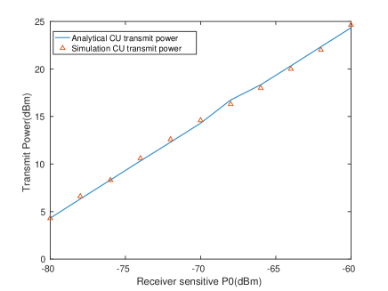
Figure 1: Transmit power of cellular UEs with $p_{0}$

As a numerical example, we plot cellular users’ transmit power in Fig. 1. The analytical result is derived from (10) and Eq.(16). It shows that the analytical result matched well with the numerical result, which validates our analyisis.

Lemma 3.

The typical D2D transmitter selects the equivalent nearest UE as a potential receiver. If the potential D2D receiver is operating in a cellular mode, D2D TU must search for another receiver. We approximate the second neighbor as the receiver under this situation. The approximate cumulative distribution function(CDF) of $\overline{R}_{d}$ can be written as

$$\Pr\left[\overline{R}_{d}<R\right]$$

$$\approx \int_{R+t}^{\infty}\left(\int_{0}^{R}f_{R_{d}}(\overline{R}_{d})d\overline{R}_{d}\right)f_{R_{d}}(r_{1})dr_{1}$$

$$+ \int_{t}^{R+t}\left(\int_{0}^{r_{1}-t}f_{R_{d}}(\overline{R}_{d})d\overline{R}_{d}\right.$$ (16)

$$+ \int_{r_{1}-t}^{R}\cdot(1-Pc)\cdot f_{R_{d}}(\overline{R}_{d})d\overline{R}_{d}$$

$$+ \left.\int_{r_{1}-t}^{R}\cdot Pc\cdot f_{R_{d_{2}}}\left(\overline{R}_{d}\right)d\overline{R}_{d}\right)f_{R_{d}}(r_{1})dr_{1},$$

where $r_{1}$is the equivalent distance from TU to the strongest BS,$t=\left(\frac{\beta}{B_{B}}\right){}^{-1/\alpha_{B}}$. $Pc$ is the probability of a D2D receiver be a CU.

Proof:

If there is no different with CUs and D2D UEs, the pdf of the distance between UEs is

$$f_{R_{d}}(r)=2\pi\lambda_{tu}r\cdotp\exp\left[-\pi\lambda_{tu}r^{2}\cdot e^{\frac{2\sigma_{D}^{2}}{\alpha_{D}^{2}}}+\frac{2\sigma_{D}^{2}}{\alpha_{D}^{2}}\right].$$ (17)

Acording to[15] , the second neighbor point is distributed as

$$f_{R_{d_{2}}}(r)=2\pi^{2}\lambda_{tu}^{2}r^{3}\cdotp\exp\left[-\pi\lambda_{tu}r^{2}\cdot e^{\frac{2\sigma_{D}^{2}}{\alpha_{D}^{2}}}+\frac{4\sigma_{D}^{2}}{\alpha_{D}^{2}}\right],$$ (18)

where $Pc$ is the probability of the potential D2D receiver operating in cellular mode, and it can be calculated as

$$Pc=\arccos\left(\frac{\overline{R}_{d}+r_{1}^{2}-t^{2}}{2\overline{R}_{d}r_{1}}\right)/\pi,$$ (19)

which concludes our proof. ∎

III-C Coverage Probability

Consider an arbitrary BS in cellular mode or UE in D2D mode. The SINR experenced at the receiver can be located in an arbitrary location and can be written as

$$\begin{array}[]{c}SINR=\frac{S_{signal}}{\underset{X_{c_{i}}\in\phi_{c}}{\sum}B_{i}^{B}\mathrm{\mathcal{H_{\mathrm{i}}^{\mathrm{B}}}}R_{B,i}^{-\alpha_{B}}+\underset{X_{d_{j}}\in\phi_{d}}{\sum}B_{j}^{D}\mathrm{\mathcal{H_{\mathrm{j}}^{\mathrm{D}}}}R_{D,j}^{-\alpha_{d}}+\eta_{c,d}}\end{array},$$ (20)

where $B_{i}^{B}=P_{C}^{i}\cdot\textrm{$A_{B}$}$ and $B^{D}=P_{D}\cdot\textrm{$A_{D}$}$ are constant based on transmission power of the $i$th CU and the TUs, $\mathcal{H_{\mathrm{i}}^{\mathrm{B}}}$and $\mathcal{H_{\mathrm{j}}^{\mathrm{D}}}$ are the lognorm fading in $i$th cellular uplink link and $j$th D2D link, $R_{B,i}$and $R_{D,i}$ are the distance from the $i$th CU and $j$th TU to the typical receiver. The Equivalence distance$\overline{R_{B}}_{i}=\mathrm{\mathcal{H}_{B,i}^{-1/\alpha_{B}}R_{B,i}}$and $\overline{R_{D}}_{j}=\mathrm{\mathcal{H}_{D,j}^{-1/\alpha_{D}}R_{D,j}}$, $\alpha_{B}$and $\alpha_{D}$ are path-loss exponent for cellular links and D2D links, respectively, $\eta_{c,d}$ is the noise for BS or receive UE.

III-C1 Cellular mode

Let us consider a typical uplink, As the underlying PPP is stationnary, without loss of generality we assume that the typical receiver is located at the original. This analysis indicates the spatially averaged performance of the network by Slivnyak’s theorem[7]. Henceforth, we only need to focus on characterizing the performance of a typical link.

Lemma 4.

The complementary cumulative distribution function(CCDF) of the SINR at a typical BS(located in the origin)

$$\begin{array}[]{l}\Pr\mathrm{\left[\textrm{SINR}>T\right]}\\ =\int_{0}^{\text{t}}\int_{\omega=-\infty}^{\infty}\left[\frac{e^{i\omega/T}-1}{2\pi i\omega}\right]\mathcal{F}_{SINR^{-1}}(\omega)d\omega f_{\overline{R}_{i}}(r)dr,\end{array}$$ (21)

where $\mathcal{F}_{SINR^{-1}}(\omega)$ denotes the conditional characteristic function of $\frac{1}{SINR}$.

$$\begin{array}[]{l}\mathcal{F}_{SINR^{-1}}(\omega)\\ =\exp\left\{-2\pi\lambda_{B}e^{\frac{2\sigma^{2}}{\alpha_{B}^{2}}}\int_{t}^{\infty}\left(1-\int_{0}^{t}\exp\left(-1\times\right.\right.\right.\\ \left.\left.\left.\frac{i\omega}{(\overline{R_{B,0}})^{\alpha_{B}(\varepsilon-1)}}r^{\alpha_{B}\varepsilon}(\tau)^{-\alpha_{B}}\right)f_{\overline{R_{i}}}(r)dr\right)\tau d\tau\right\}\\ \times\exp\left\{-\pi(1-q)\lambda_{u}e^{\frac{2\sigma^{2}}{\alpha_{B}^{2}}}\int_{t}^{\infty}\left(1-\exp\left(-1\times\right.\right.\right.\\ \left.\left.\frac{i\omega A_{B}^{\varepsilon}P_{d}}{P_{0}\cdot(\overline{R_{B,0}})^{\alpha_{B}(\varepsilon-1)}}(L)^{-\alpha_{B}}\right)LdL\right\}\\ \times\exp\left(-\frac{i\omega\eta}{\frac{P_{0}}{(\mathrm{A_{B}})^{\varepsilon-1}}\cdot(\overline{R_{B,0}})^{\alpha_{B}(\varepsilon-1)}}\right).\end{array}$$ (22)

Proof:

Conditioning on the strongest BS being at a distance $R_{B,0}$ from the typical CU, the Equivalence distance$\overline{R_{B,0}}=\mathrm{\mathcal{H}_{B}^{-1/\alpha_{B}}R_{B,0}}$ $\left(\overline{R_{B,0}}\leq\left(\frac{\beta}{B_{B}}\right){}^{-1/\alpha_{B}}\right)$, probability of coverage averaged over the plane is

$$\begin{array}[]{cl}p_{c}(T,\lambda)&=\Pr[SINR>T]\\ &=\Pr[\frac{1}{SINR}<\frac{1}{T}]\\ &=\int_{0}^{\text{t}}\Pr[\left.\frac{1}{SINR}<\frac{1}{T}\right|\overline{R_{B,0}}]f_{\overline{R_{i}}}(r)dr\end{array},$$ (23)

where $i=\sqrt{-1}$ is the imaginary unit; The inner intergral is the conditional PDF of $\frac{1}{SINR}$;$\mathcal{F}_{SINR^{-1}}(\omega)$ denotes the conditional characteristic function of $\frac{1}{SINR}$which can be written by

$$\mathcal{F}_{SINR^{-1}}(\omega)$$ (24)

$$= \mathbb{E\mathrm{{}_{\phi}}}\left[\left.\exp\left(-i\omega\frac{1}{SINR}\right)\right|\overline{R_{B,0}}\right]$$

$$= E_{\phi_{c}}\left[\exp\left(-\frac{i\omega}{\frac{P_{0}}{(\mathrm{A_{B}})^{\varepsilon-1}}\cdot(\overline{R_{B,0}})^{\alpha_{B}(\varepsilon-1)}}(I_{C})\right)\right]$$

$$\times \mathbb{E}{}_{\phi_{d}}\left[\exp\left(-\frac{i\omega}{\frac{P_{0}}{(\mathrm{A_{B}})^{\varepsilon-1}}\cdot(\overline{R_{B,0}})^{\alpha_{B}(\varepsilon-1)}}(I_{D})\right)\right]$$

$$\times \exp\left(-\frac{i\omega\eta}{\frac{P_{0}}{(\mathrm{A_{B}})^{\varepsilon-1}}\cdot(\overline{R_{B,0}})^{\alpha_{B}(\varepsilon-1)}}\right),$$

and using the definition of the Laplace transform yields, from [7] we have

$$\mathcal{L_{\mathrm{I_{c}}}\mathrm{(\mathit{s})}} = \mathbb{E}{}_{\phi_{c}}\left[\exp(-\mathit{sI_{c}})\right]$$ (25)

$$= \exp\left\{-2\pi\lambda_{B}e^{\frac{2\sigma^{2}}{\alpha_{B}^{2}}}\int_{\overline{R_{B,0}}}^{\infty}\left(1-\int_{0}^{t}\exp\left(-1\times\right.\right.\right.$$

$$\left.\left.\left.sP_{0}A_{B}^{(1-\varepsilon)}r^{\alpha_{B}\varepsilon}(\tau)^{-\alpha_{B}}\right)f_{\overline{R_{i}}}(r)dr\right)\tau d\tau\right\},$$

Plugging in $s=\frac{i\omega}{\frac{P_{0}}{(\mathrm{A_{B}})^{\varepsilon-1}}\cdot(\overline{R_{B,0}})^{\alpha_{B}(\varepsilon-1)}}$ gives.

$$\mathbb{E}{}_{\phi_{c}}[\exp(-\frac{i\omega}{\frac{P_{0}}{(\mathrm{A_{B}})^{\varepsilon-1}}\cdot(\overline{R_{B,0}})^{\alpha_{B}(\varepsilon-1)}}(I_{C}))$$ (26)

$$= \exp\left\{-2\pi\lambda_{B}e^{\frac{2\sigma^{2}}{\alpha_{B}^{2}}}\int_{t}^{\infty}\left(1-\int_{0}^{t}\exp\left(-1\times\right.\right.\right.$$

$$\left.\left.\left.\frac{i\omega}{(\overline{R_{B,0}})^{\alpha_{B}(\varepsilon-1)}}r^{\alpha_{B}\varepsilon}(\tau)^{-\alpha_{B}}\right)f_{\overline{R_{i}}}(r)dr\right)\tau d\tau\right\},$$

Similarly, the term $\mathbb{E}{}_{\phi_{d}}\left[\exp\left(-\frac{i\omega}{\frac{P_{0}}{(\mathrm{A_{B}})^{\varepsilon-1}}\cdot(\overline{R_{B,0}})^{\alpha_{B}(\varepsilon-1)}}(I_{D})\right)\right]$ in Eq.(25) can be written by

$$\mathbb{E}{}_{\phi_{d}}[\exp(-\frac{i\omega}{\frac{P_{0}}{(\mathrm{A_{B}})^{\varepsilon-1}}\cdot(\overline{R_{B,0}})^{\alpha_{B}(\varepsilon-1)}}(I_{D}))]$$ (27)

$$= \mathbb{E}{}_{\phi_{d}}[\underset{X_{d_{i}}\in\phi_{d}}{\prod}[\exp(-\frac{i\omega A_{B}^{\varepsilon}P_{d}}{P_{0}\cdot(\overline{R_{B,0}})^{\alpha_{B}(\varepsilon-1)}}(\overline{R_{C,i}})^{-\alpha_{B}})]]$$

$$= \exp\left\{-\pi(1-q)\lambda_{u}e^{\frac{2\sigma^{2}}{\alpha_{B}^{2}}}\int_{t}^{\infty}\left(1-\right.\right.$$

$$\left.\left.\exp(-\frac{i\omega A_{B}^{\varepsilon}P_{d}}{P_{0}\cdot(\overline{R_{B,0}})^{\alpha_{B}(\varepsilon-1)}}(L)^{-\alpha_{B}}\right)LdL\right\}.$$

where $\lambda_{u}$is the intensity of Users,$R_{D,i}^{\alpha}$is the distance from $i$th TU to typical BS. ∎

III-C2 Coverage Probability of D2D Mode

Now let us consider a typical D2D link. As the underlying PPP is stationary, without loss of generality, we assume that the typical receiver is located at the original.

Lemma 5.

The CCDF of the SINR at a typical D2D UE(located in the origin)

$$\begin{array}[]{l}\Pr[\textrm{SINR}>T]\\ =\int_{0}^{\infty}\int_{\omega=-\infty}^{\infty}\left[\frac{e^{i\omega/T}-1}{2\pi i\omega}\right]\mathcal{F}_{SINR^{-1}}(\omega)d\omega f_{\overline{R_{d}}}(r)dr,\end{array}$$ (28)

where $\mathcal{F}_{SINR^{-1}}(\omega)$ denotes the conditional characteristic function of $\frac{1}{SINR}$.

$$\begin{array}[]{l}\mathcal{F}_{SINR^{-1}}(\omega)\\ =\exp\left\{-2\pi\lambda_{B}e^{\frac{2\sigma^{2}}{\alpha_{B}^{2}}}\int_{0}^{\infty}\left(1-\int_{0}^{t}\exp\left(-1\times\right.\right.\right.\\ \left.\left.\left.\frac{i\omega}{P_{d}(\overline{R_{d,0}})^{-\alpha_{d}}}P_{0}A_{B}^{-\varepsilon}r^{\alpha_{B}\varepsilon}(\tau)^{-\alpha_{B}}\right)f_{\overline{R_{i}}}(r)dr\right)\tau d\tau\right\}\\ \times\exp\left\{-\pi(1-q)\lambda_{u}e^{\frac{2\sigma_{d}^{2}}{\alpha_{d}^{2}}}\int_{\overline{R_{d,0}}}^{\infty}\left(1-\exp\left(-1\times\right.\right.\right.\\ \left.\left.\frac{i\omega}{(\overline{R_{d,0}})^{-\alpha_{d}}}(L)^{-\alpha_{B}}\right)LdL\right\}\\ \times\exp\left(-\frac{i\omega\eta_{d}}{P_{d}A_{D}(\overline{R_{d,0}})^{-\alpha_{d}}}\right)\end{array}$$ (29)

and

$$f_{\overline{R_{d}}}(r)=\frac{\partial\Pr\left[\overline{R}_{d}>R\right]}{\partial\overline{R}_{d}}.$$ (30)

Proof:

The proof is very similar to that for the cellular mode, and hence we omit the proof here for brevity. ∎

IV Simulations and Discussion

In this section, we use numerical results to validate our results on the performance of the considered D2D-enabled UL cellular network. According to the 3GPP LTE specifications[16], we set the BS intensity to $\lambda_{B}=5\,\textrm{BSs/k$m^{2}$}$, which results in an average inter-site distance of about 500 m. The UE intensity is chosen as $\lambda=300\,\textrm{UEs/k$m^{2}$}$ [17]. The transmit power of each BS is $P_{B}=46\,\textrm{dBm}$, the transmit power of D2D transmitter is $10\,\textrm{dBm}$, the path-loss exponents are $\alpha_{c}=3.75$, $\alpha_{d}=3.75$, and the path-loss constants are $A_{B}=10^{-3.29}$, $A_{D}=10^{-5.578}$. The threshold for selecting cellular mode communication is set to $\beta=-65\textrm{dBm}$. The logmormal shadowing standard deviation is $8\,\textrm{dB}$ between UEs to BSs and $7\,\textrm{dB}$ between UEs to UEs. The noise power is set to $-95\,\textrm{dBm}$ for a UE receiver and $-114\,\textrm{dBm}$ for a BS receiver, respectively.

IV-A The Results on the Coverage Probability

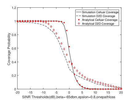
Figure 2: Coverage probabality

In Fig.2, we plot the coverage probability for both a typical cellular UE and a typical D2D UE. From this figure, we can draw the following observations:

• Our analytical results match well with the simulation results, which validates our analysis and shows that the adopted model accurately captures the features of D2D communications.

• The coverage probability decreases with the increase of SINR threshold, because a higher SINR requirement decreases the coverage probability.

• In the D2D mode, the analytical results is shown to be larger than the simulation resutls. This is becuase we approximate the distance from a typical D2D TU to a typical D2D RU as that from a second nearest D2D UE to such typical D2D RU, when the nearest D2D UE to such typical D2D RU selects the cellular mode. However, the real distance from a typical D2D TU to a typical D2D RU could be larger than the approximate distance used in our analysis addressed in subsection 3.2.

IV-B The Results on the ASE

In Fig.3, we display the ASE results with $\gamma_{0}=0\,\textrm{dB}$. Since $A^{\textrm{ASE}}(\lambda_{B},\lambda_{u},\gamma_{0})$ is a function of the coverage probablity, which has been validated in Fig.2, we only show analytical results in Fig.3.

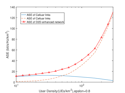
Figure 3: ASE with the different density of users

From Fig.3, we can draw the following observations:

• The total ASE increases with the increase of the intensity of UE. This is because the spectral reuse factor increases with the number of UEs in the network.

• When the intensity of UE is around $\lambda=100\,\textrm{UEs/k$m^{2}$}$, the enabled-D2D links have a comparable contribution to the total ASE as the cellular links. This is because there are around 1/3 UEs operating in D2D mode and base on the coverage probability in D2D tier there are around 1/3 D2D users are given a acceptable service ($\text{SINR}>0dB$), and hence they make roughly equal contributions to the ASE performance.

• When the network is dense enough, i.e., $\lambda_{u}\in\left[50,250\right]\textrm{UEs/k$m^{2}$}$, which is the practical range of intensity for the existing 4G network and the futrue 5G network[2], the total ASE performance increases quickly, while the ASE of the cellular network stays on top of $5\,\textrm{bps/Hz/k$m^{2}$}$.

IV-C The Performance Impact of $\beta$ on the ASE

In this subsection, we investigate the performance impact of $\beta$ on the ASE, which is shown in Fig. 4. From this figure, we can see there is a tradeoff in the coverage probability of the cellular mode. This means that with a proper choice of $\beta$, enabling D2D communications not only can improve the ASE of the network, but also can improve the coverage for cellular users.

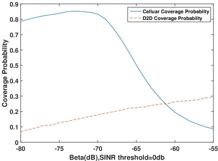
Figure 4: Coverage probability with different beta

This is because the cell edge UEs in the conventional UL cellular network will be offloaded to D2D modes to enjoy a better coverage performance.

V Conclusion

In this paper, we provided a stochastic geometry based theoretical framework to analyze the performance of a D2D underlaid uplink cellular network. In particular, we considered lognormal shadowing fading, a practical D2D mode selection criterion based on the maximum DL received power and the D2D power control mechanism. Our results showed that enabling D2D communications in cellular networks can improve the total ASE, while having a minor performance impact on the cellular network. As future work, a more practical path loss model incorporating both line-of-sight and non-line-of-sight transmissions will be considered, and we will find the optimal parameters for the network that can achieve the maximum total ASE.

References

- [1] Cisco Visual Networking Index Cisco. Global mobile data traffic forecast update, 2013–2018. white paper, 2014.
- [2] D. Lopez-Perez, M. Ding, H. Claussen, and A. H. Jafari. Towards 1 gbps/ue in cellular systems: Understanding ultra-dense small cell deployments. IEEE Communications Surveys Tutorials, 17(4):2078–2101, Fourthquarter 2015.
- [3] J. Liu, H. Nishiyama, N. Kato, and J. Guo. On the outage probability of device-to-device-communication-enabled multichannel cellular networks: An rss-threshold-based perspective. IEEE Journal on Selected Areas in Communications, 34(1):163–175, Jan 2016.
- [4] H. ElSawy, E. Hossain, and M. S. Alouini. Analytical modeling of mode selection and power control for underlay d2d communication in cellular networks. IEEE Transactions on Communications, 62(11):4147–4161, Nov 2014.
- [5] Namyoon Lee, Xingqin Lin, Jeffrey G Andrews, and Robert W Heath. Power control for d2d underlaid cellular networks: Modeling, algorithms, and analysis. IEEE Journal on Selected Areas in Communications, 33(1):1–13, 2015.
- [6] X. Lin, J. G. Andrews, and A. Ghosh. Spectrum sharing for device-to-device communication in cellular networks. IEEE Transactions on Wireless Communications, 13(12):6727–6740, Dec 2014.
- [7] J. G. Andrews, F. Baccelli, and R. K. Ganti. A tractable approach to coverage and rate in cellular networks. IEEE Transactions on Communications, 59(11):3122–3134, November 2011.
- [8] T. D. Novlan, H. S. Dhillon, and J. G. Andrews. Analytical modeling of uplink cellular networks. IEEE Transactions on Wireless Communications, 12(6):2669–2679, June 2013.
- [9] Mugen Peng, Yuan Li, Tony QS Quek, and Chonggang Wang. Device-to-device underlaid cellular networks under rician fading channels. Wireless Communications, IEEE Transactions on, 13(8):4247–4259, 2014.
- [10] H. Sun, M. Wildemeersch, M. Sheng, and T. Q. S. Quek. D2d enhanced heterogeneous cellular networks with dynamic tdd. IEEE Transactions on Wireless Communications, 14(8):4204–4218, Aug 2015.
- [11] G. George, R. K. Mungara, and A. Lozano. An analytical framework for device-to-device communication in cellular networks. IEEE Transactions on Wireless Communications, 14(11):6297–6310, Nov 2015.
- [12] D. Xenakis, M. Kountouris, L. Merakos, N. Passas, and C. Verikoukis. Performance analysis of network-assisted d2d discovery in random spatial networks. IEEE Transactions on Wireless Communications, 15(8):5695–5707, Aug 2016.
- [13] M. Ding, D. López-Pérez, and G. Mao. A new capacity scaling law in ultra-dense networks. arXiv:1704.00399 [cs.NI], Apr. 2017.
- [14] B. Blaszczyszyn, M. K. Karray, and H. P. Keeler. Using poisson processes to model lattice cellular networks. In 2013 Proceedings IEEE INFOCOM, pages 773–781, April 2013.
- [15] M. Haenggi. On distances in uniformly random networks. IEEE Transactions on Information Theory, 51(10):3584–3586, Oct 2005.
- [16] 3GPP. "tr 36.828 (v11.0.0): Further enhancements to lte time division duplex (tdd) for downlink-uplink (dl-ul) interference management and traffic adaptation,". Jun 2012.
- [17] Ming Ding, Peng Wang, David López-Pérez, Guoqiang Mao, and Zihuai Lin. Performance impact of los and nlos transmissions in small cell networks. IEEE Trans. Wireless Commun.,Online. Available: http://arxiv. org/pdf/1503.04251. pdf, 2015.