The even exciton series in Cu₂O

Abstract

Recent investigations of excitonic absorption spectra in cuprous oxide ($\mathrm{Cu_{2}O}$) have shown that it is indispensable to account for the complex valence band structure in the theory of excitons. In $\mathrm{Cu_{2}O}$ parity is a good quantum number and thus the exciton spectrum falls into two parts: The dipole-active exciton states of negative parity and odd angular momentum, which can be observed in one-photon absorption ($\Gamma_{4}^{-}$ symmetry) and the exciton states of positive parity and even angular momentum, which can be observed in two-photon absorption ($\Gamma_{5}^{+}$ symmetry). The unexpected observation of $D$ excitons in two-photon absorption has given first evidence that the dispersion properties of the $\Gamma_{5}^{+}$ orbital valence band is giving rise to a coupling of the yellow and green exciton series. However, a first theoretical treatment by Ch. Uihlein et al. [Phys. Rev. B 23, 2731 (1981)] was based on a simplified spherical model. The observation of $F$ excitons in one-photon absorption is a further proof of a coupling between yellow and green exciton states. Detailed investigations on the fine structure splitting of the $F$ exciton by F. Schweiner et al. [Phys. Rev. B 93, 195203 (2016)] have proved the importance of a more realistic theoretical treatment including terms with cubic symmetry. In this paper we show that the even and odd parity exciton system can be consistently described within the same theoretical approach. However, the Hamiltonian of the even parity system needs, in comparison to the odd exciton case, modifications to account for the very small radius of the yellow and green $1S$ exciton. In the presented treatment we take special care of the central-cell corrections, which comprise a reduced screening of the Coulomb potential at distances comparable to the polaron radius, the exchange interaction being responsible for the exciton splitting into ortho and para states, and the inclusion of terms in the fourth power of $p$ in the kinetic energy being consistent with $O_{\mathrm{h}}$ symmetry. Since the yellow $1S$ exciton state is coupled to all other states of positive parity, we show how the central-cell corrections affect the whole even exciton series. The close resonance of the $1S$ green exciton with states of the yellow exciton series has a strong impact on the energies and oscillator strengths of all implied states. The consistency between theory and experiment with respect to energies and oscillator strengths for the even and odd exciton system in $\mathrm{Cu_{2}O}$ is a convincing proof for the validity of the applied theory.

I Introduction 

Excitons are the quanta of fundamental optical excitations in both insulators and semiconductors in the visible and ultraviolet spectrum of light. The Coulomb interaction between electron and hole leads to a hydrogen-like series of excitonic states Knox (1963). Cuprous oxide $\left(\mathrm{Cu_{2}O}\right)$ is a prime example where one can even identify four different excitonic series (yellow, green, blue, and violet) being related to the two topmost valence bands and the two lowest conduction bands Kazimierczuk et al. (2014). Recently, the yellow series could be followed up to a spectacular high principal quantum number of $n=25$ Kazimierczuk et al. (2014). This outstanding experiment has launched the new field of research of giant Rydberg excitons and led to a variety of new theoretical and experimental investigations on the topic of excitons in $\mathrm{Cu_{2}O}$ Thewes et al. (2015); Aßmann et al. (2016); Schweiner et al. (2017a, 2016a); Grünwald et al. (2016); Feldmaier et al. (2016); Schöne et al. (2016); Schweiner et al. (2016b, 2017b); Heckötter et al. (2017); Zielińska-Raczyńska et al. (2017); Schweiner et al. (2016c); Zielińska-Raczyńska et al. (2016a, b); Schweiner et al. (2017c).

$\mathrm{Cu_{2}O}$ has octahedral symmetry $O_{\mathrm{h}}$ so that the symmetry of the bands can be assigned by the irreducible representations $\Gamma_{i}^{\pm}$ of $O_{\mathrm{h}}$. The yellow and green exciton series share the same threefold degenerate $\Gamma_{5}^{+}$ orbital valence band state. This state splits due to spin-orbit interaction into an upper twofold degenerate $\Gamma_{7}^{+}$ valence band (yellow series) and a lower fourfold degenerate $\Gamma_{8}^{+}$ valence band (green series). The band structure of both bands is essentially determined by the anisotropic dispersion properties of the orbital state. The threefold degeneracy of the orbital state is lifted as soon as a non-zero $k$ vector gets involved, with new eigenvectors depending on the orientation of $\bm{k}$. A consequence of the splitting of the orbital state is a partial quenching of the spin-orbit interaction. This $\bm{k}$ dependent quenching is not only responsible for a remarkable non-parabolicity of the two top valence bands but leads likewise to a $\bm{k}$ dependent mixing of the $\Gamma_{7}^{+}$ and $\Gamma_{8}^{+}$ Bloch states and can thus cause a mixing of the yellow and green exciton series. A mixing of both series is favored by the large Rydberg energy of approximately $100\,\mathrm{meV}$, a corresponding large exciton extension in $k$ space and the small spin-orbit splitting of only $130\,\mathrm{meV}$.

A Hamiltonian that is able to cope with a coupled system of yellow and green excitons must take explicit care of the dispersion properties of the orbital valence band state and has to include the spin-orbit interaction. Such a kind of Hamiltonian was first introduced by Uihlein et al. Uihlein et al. (1981) for explaining the unexpected fine structure splitting observed in the two-photon absorption spectrum of $\mathrm{Cu_{2}O}$. They used a simplified spherical dispersion model for the $\Gamma_{5}^{+}$ orbital valence band with an identical splitting into longitudinal and transverse states independent of the orientation of $\bm{k}$. This simplification had the appealing advantage that the total angular momentum remains a good quantum number so that the exciton problem could be reduced to calculate the eigenvalues of a system of coupled radial wave functions. A problem in their paper is the incorrect notation of the $1S$ green and $2S$ yellow excitons states. Both notations need to be exchanged to be consistent with their calculations. Although the spherical model can explain many details of the experimental findings, one has to be aware of its limitations. A more realistic Hamiltonian being compliant with the real band structure by including terms of cubic symmetry has already proved its validity by explaining the puzzling fine structure of the odd parity states in $\mathrm{Cu_{2}O}$ Schweiner et al. (2016b). The intention of this paper is to show that the same kind of Hamiltonian can likewise describe the fine splitting of the even parity excitons.

However, when comparing the even parity and odd parity exciton systems, it is obvious that the even exciton system is a much more challenging problem. One reason for this is the close resonance of the green $1S$ exciton with the even parity states of the yellow series with principal quantum number $n\geq 2$. This requires a very careful calculation of the binding energy of the green $1S$ exciton. Furthermore, the binding energy of the yellow $1S$ exciton is much larger than expected from a simple hydrogen like series, inter alia, due to a less effective screening of the Coulomb potential at distances comparable to the polaron radius. Moreover, a breakdown of the electronic screening is expected at even much shorter distances, but a proper treatment is exceeding the limits of the continuum approximation. Hence, we introduce in this paper a $\delta$-function like central cell correction term that should account for all kinds of short range perturbations affecting the immediate neighborhood of the central cell. The magnitude of this term is treated as a free parameter that can be adjusted to the experimental findings. It is important to note that a change of this parameter leads to a significant shift of the green $1S$ exciton with respect to the higher order states of the yellow series and has therefore a high impact on the energies and the compositions of the resulting coupled exciton states. Taking this in mind it is fundamental that one can likewise achieve a match to the relative oscillator strengths of the involved states.

Dealing with the even parity system of $\mathrm{Cu_{2}O}$ is also confronting us with the problem of a proper treatment of the $1S$ exciton with respect to its very small radius since a small exciton radius means a large extension of the exciton in $k$ space. The challenge is therefore to meet the band structure of the valence band in a much larger vicinity of the $\Gamma$ point. For coping with this situation, we include in the kinetic energy of the hole all terms in the fourth power of $p$ being compliant with the octahedral symmetry of $\mathrm{Cu_{2}O}$. The parameters of these terms are carefully adjusted to get a best fit to the band structure in the part of the $k$ space being relevant for the $1S$ exciton.

Despite of all these modifications, it is important to note that the Hamiltonian is essentially the same as the one being applied to the odd exciton system Schweiner et al. (2016b). The fundamental modifications presented in this paper are irrelevant for the odd parity system because of their $\delta$ function like nature or their specific form affecting only exciton states with a small radius. Hence, we present a consistent theoretical model for the complete exciton spectrum of $\mathrm{Cu_{2}O}$.

Comparing our results to experimental data, we can prove very good agreement as regards not only the energies but also the oscillator strengths since our method of solving the Schrödinger equation allows us also to calculate relative oscillator strengths for one-photon and two-photon absorption. This agreement between theory and experiment is important not only for the investigation of exciton spectra in electric or combined electric and magnetic fields. A correct theoretical description of excitons is indispensable if Rydberg excitons will be used in the future in quantum information technology, or used to attain a deeper understanding of quasi-particle interactions in semiconductors Zielińska-Raczyńska et al. (2016b); Kazimierczuk et al. (2014). Furthermore, this agreement is a prerequisite for a future search for exceptional points in the exciton spectrum Feldmaier et al. (2016).

The paper is organized as follows: Having presented the Hamiltonian of excitons in $\mathrm{Cu_{2}O}$ when considering the complete valence band structure Sec. II, we discuss all corrections to this Hamiltonian due to the small radius of the $1S$ exciton in Sec. III. In Sec. IV we show how to solve the Schrödinger equation using a complete basis and how to calculate relative oscillator strengths for one-photon and two-photon absorption. In Sec. V we discuss the complete yellow and green exciton spectrum of $\mathrm{Cu_{2}O}$ paying attention to the exciton states with a small principal quantum number and especially to the green $1S$ exciton state. Finally, we give a short summary and outlook in Sec. VI.

II Hamiltonian 

In this section we present the Hamiltonian of excitons in $\mathrm{Cu_{2}O}$, which accounts for the complete valence band structure of this semiconductor. This Hamiltonian describes the exciton states of odd parity with a principal quantum number $n\geq 3$ very well Schweiner et al. (2016b, 2017b). However, for the exciton states of even parity and for the $2P$ exciton corrections to this Hamiltonian are needed, which will be described in Sec. III.

The lowest $\Gamma_{6}^{+}$ conduction band in $\mathrm{Cu_{2}O}$ is almost parabolic in the vicinity of the $\Gamma$ point and the kinetic energy can be described by the simple expression

$$H_{\mathrm{e}}\!\left(\bm{p}_{\mathrm{e}}\right)=\frac{\bm{p}_{\mathrm{e}}^{2}}{2m_{\mathrm{e}}},$$ (1)

with the effective electron mass $m_{\mathrm{e}}$. Since $\mathrm{Cu_{2}O}$ has cubic symmetry, we use the irreducible representations $\Gamma_{i}^{\pm}$ of the cubic group $O_{\mathrm{h}}$ to assign the symmetry of the bands.

Due to interband interactions and nonparabolicities of the three uppermost valence bands in $\mathrm{Cu_{2}O}$, the kinetic energy of the hole is given by the more complex expression Schöne et al. (2016); Schweiner et al. (2016b, 2017b),

$$H_{\mathrm{h}}\!\left(\bm{p}_{\mathrm{h}}\right) = H_{\mathrm{so}}+\left(1/2\hbar^{2}m_{0}\right)\left\{\hbar^{2}\left(\gamma_{1}+4\gamma_{2}\right)\bm{p}_{\mathrm{h}}^{2}\right.\phantom{\frac{1}{1}}$$ (2)

$$+ 2\left(\eta_{1}+2\eta_{2}\right)\bm{p}_{\mathrm{h}}^{2}\left(\bm{I}\cdot\bm{S}_{\mathrm{h}}\right)\phantom{\frac{1}{1}}$$

$$- 6\gamma_{2}\left(p_{\mathrm{h}1}^{2}\bm{I}_{1}^{2}+\mathrm{c.p.}\right)-12\eta_{2}\left(p_{\mathrm{h}1}^{2}\bm{I}_{1}\bm{S}_{\mathrm{h}1}+\mathrm{c.p.}\right)\phantom{\frac{1}{1}}$$

$$- 12\gamma_{3}\left(\left\{p_{\mathrm{h}1},p_{\mathrm{h}2}\right\}\left\{\bm{I}_{1},\bm{I}_{2}\right\}+\mathrm{c.p.}\right)\phantom{\frac{1}{1}}$$

$$- \left.12\eta_{3}\left(\left\{p_{\mathrm{h}1},p_{\mathrm{h}2}\right\}\left(\bm{I}_{1}\bm{S}_{\mathrm{h}2}+\bm{I}_{2}\bm{S}_{\mathrm{h}1}\right)+\mathrm{c.p.}\right)\right\}\phantom{\frac{1}{1}}$$

with $\left\{a,b\right\}=\frac{1}{2}\left(ab+ba\right)$, the free electron mass $m_{0}$, and c.p. denoting cyclic permutation. The quasi-spin $I=1$ describes the threefold degenerate valence band and is a convenient abstraction to denote the three orbital Bloch functions $xy$, $yz$, and $zx$ Luttinger (1956). The parameters $\gamma_{i}$, which are called the first three Luttinger parameters, and the parameters $\eta_{i}$ describe the behavior and the anisotropic effective mass of the hole in the vicinity of the $\Gamma$ point. The spin-orbit coupling, which enters Eq. (2), is given by

$$H_{\mathrm{so}}=\frac{2}{3}\Delta\left(1+\frac{1}{\hbar^{2}}\bm{I}\cdot\bm{S}_{\mathrm{h}}\right).$$ (3)

In a first approximation, the interaction between the electron and the hole is described by a screened Coulomb potential

$$V\!\left(\bm{r}_{e}-\bm{r}_{h}\right)=-\frac{e^{2}}{4\pi\varepsilon_{0}\varepsilon_{\mathrm{s}1}}\frac{1}{\left|\bm{r}_{e}-\bm{r}_{h}\right|}$$ (4)

with the dielectric constant $\varepsilon_{\mathrm{s}1}=7.5$. For small relative distances $r=\left|\bm{r}\right|=\left|\bm{r}_{e}-\bm{r}_{h}\right|$ corrections to this potential and to the kinetic energies $H_{\mathrm{e}}\left(\bm{p}_{\mathrm{e}}\right)$ and $H_{\mathrm{h}}\left(\bm{p}_{\mathrm{h}}\right)$ are needed, which will be described in Sec. III and which will be denoted here by $V^{\mathrm{CCC}}$.

After introducing relative and center of mass coordinates Schmelcher and Cederbaum (1992) and setting the position and momentum of the center of mass to zero, the complete Hamiltonian of the relative motion finally reads Lipari and Altarelli (1977); Uihlein et al. (1981)

$$H = E_{\mathrm{g}}+V\!\left(\bm{r}\right)+H_{\mathrm{e}}\!\left(\bm{p}\right)+H_{\mathrm{h}}\!\left(\bm{p}\right)+V_{\mathrm{CCC}}$$ (5)

with the energy $E_{\mathrm{g}}$ of the band gap.

Note that by setting the total momentum to zero, we neglect polariton effects, even though in experiments the polaritonic part is always present. However, when considering the experimental results of Refs. Dasbach et al. (2003, 2005, 2004), the polariton effect on the $1S$ exciton is on the order of tens of $\mu\mathrm{eV}$ and, hence, much smaller than the energy shifts considered here. Furthermore, in Ref. Andreani (2014) criteria for the experimental observability of polariton effects are given. Inserting the material parameters of $\mathrm{Cu_{2}O}$ and the experimental linewidths of the exciton states observed in Refs. Kazimierczuk et al. (2014); Thewes et al. (2015), it can be shown that polariton effects are not observable for the exciton states of $n\geq 2$. We will discuss this in greater detail in a future work.

III Central-cell corrections 

Due to its small radius, the $1S$ exciton in $\mathrm{Cu_{2}O}$ is an exciton intermediate between a Frenkel and a Wannier exciton Knox (1963). Hence, appropriate corrections are needed to describe this exciton state correctly. The corrections, which allow for the best possible description of the exciton problem within the continuum approximation of the solid, are called central-cell corrections and have first been treated by Uihlein et al Fröhlich et al. (1979); Uihlein et al. (1981) and Kavoulakis et al Kavoulakis et al. (1997) for $\mathrm{Cu_{2}O}$. While Uihlein et al Uihlein et al. (1981) accounted for these corrections only in a simplified way by using a semi-empirical contact potential $V=-V_{0}\delta\!\left(\bm{r}\right)$, the treatment of Kavoulakis et al Kavoulakis et al. (1997) did non account for the band structure and the effect of the central-cell corrections was discussed only on the $1S$ state and only using perturbation theory. By considering the complete valence band structure of $\mathrm{Cu_{2}O}$ in combination with a non-perturbative treatment of the central-cell corrections, we present a more accurate treatment of the whole yellow exciton series in $\mathrm{Cu_{2}O}$. Corrections beyond the frame of the continuum approximation will not be treated here. However, these corrections may describe remaining small deviations between experimental and theoretical results.

The central-cell corrections as discussed in Ref. Kavoulakis et al. (1997) comprise three effects, which are (i) the appearance of terms of higher-order in the momentum $\bm{p}$ in the kinetic energies of electron and hole, (ii) the momentum- and frequency-dependence of the dielectric function $\varepsilon$, and (iii) the appearance of an exchange interaction, which depends on the momentum of the center of mass.

III.1 Band structure of Cu₂O 

Since the radius of the yellow $1S$ exciton is small, the extension of its wave function in momentum space is accordingly large. Hence, we have to consider terms of the fourth power of $\bm{p}$ in the kinetic energy of the electron and the hole. The inclusion of $p^{4}$ terms in Eqs. (1) and (2) leads to an extended and modified Hamiltonian in the sense of Altarelli, Baldereschi and Lipari Baldereschi and Lipari (1971, 1974, 1973); Lipari and Altarelli (1977); Altarelli and Lipari (1977) or Suzuki and Hensel Suzuki and Hensel (1974).

The extended Hamiltonian must be compatible with the symmetry $O_{\mathrm{h}}$ of the crystal and transform according to the irreducible representation $\Gamma_{1}^{+}$. All the terms of the fourth power of $\bm{p}$ span a fifteen-dimensional space with the basis functions

$$p_{i}^{4},\quad p_{i}^{3}p_{j},\quad p_{i}^{2}p_{j}^{2},\quad p_{i}p_{j}p_{k}^{2}$$ (6)

with $i,j,k\in\{1,2,3\}$ and $i\neq j\neq k\neq i$. Including the quasi spin $I$ and using group theory, one can find six linear combinations of $p^{4}$ terms, which transform according to $\Gamma_{1}^{+}$ Koster et al. (1963) (see Appendix A). Using the results of Appendix A, we can write the kinetic energy of the electron and the hole as

$$H_{\mathrm{e}}\!\left(\bm{p}_{\mathrm{e}}\right) = \frac{1}{2\hbar^{2}m_{\mathrm{e}}}\left\{\left(\hbar^{2}+\lambda_{1}a^{2}\bm{p}_{\mathrm{e}}^{2}\right)\bm{p}_{\mathrm{e}}^{2}+\lambda_{2}a^{2}\left[p_{\mathrm{e}1}^{2}p_{\mathrm{e}2}^{2}+\mathrm{c.p.}\right]\right\}$$ (7)

and

$$H_{\mathrm{h}}\!\left(\bm{p}_{\mathrm{h}}\right) = H_{\mathrm{so}}+\frac{1}{2\hbar^{4}m_{0}}\left\{\left(\gamma_{1}+4\gamma_{2}\right)\hbar^{2}\left(\hbar^{2}+\xi_{1}a^{2}\bm{p}_{\mathrm{h}}^{2}\right)\bm{p}_{\mathrm{h}}^{2}+\xi_{2}a^{2}\hbar^{2}\left[p_{\mathrm{h}1}^{2}p_{\mathrm{h}2}^{2}+\mathrm{c.p.}\right]\right.$$ (8)

$$- 6\gamma_{2}\left(\hbar^{2}+\xi_{3}a^{2}\bm{p}_{\mathrm{h}}^{2}\right)\left[p_{\mathrm{h}1}^{2}\bm{I}_{1}^{2}+\mathrm{c.p.}\right]-12\gamma_{3}\left(\hbar^{2}+\xi_{4}a^{2}\bm{p}_{\mathrm{h}}^{2}\right)\left[p_{\mathrm{h}1}p_{\mathrm{h}2}\left\{\bm{I}_{1},\bm{I}_{2}\right\}+\mathrm{c.p.}\right]$$

$$+ 2\left(\eta_{1}+2\eta_{2}\right)\hbar^{2}\left[\bm{p}_{\mathrm{h}}^{2}\;\bm{I}\cdot\bm{S}_{\mathrm{h}}\right]-12\eta_{2}\hbar^{2}\left[p_{\mathrm{h}1}^{2}\bm{I}_{1}\bm{S}_{\mathrm{h}1}+\mathrm{c.p.}\right]-12\eta_{3}\hbar^{2}\left[p_{\mathrm{h}1}p_{\mathrm{h}2}\left(\bm{I}_{1}\bm{S}_{\mathrm{h}2}+\bm{I}_{2}\bm{S}_{\mathrm{h}1}\right)+\mathrm{c.p.}\right]$$

$$- \left.6\xi_{5}a^{2}\left[\left(p_{\mathrm{h}1}^{4}+6p_{\mathrm{h}2}^{2}p_{\mathrm{h}3}^{2}\right)\bm{I}_{1}^{2}+\mathrm{c.p.}\right]-12\xi_{6}a^{2}\left[\left(p_{\mathrm{h}1}^{2}+p_{\mathrm{h}2}^{2}-6p_{\mathrm{h}3}^{2}\right)p_{\mathrm{h}1}p_{\mathrm{h}2}\left\{\bm{I}_{1},\,\bm{I}_{2}\right\}+\mathrm{c.p.}\right]\right\}$$

with the lattice constant $a$ and the unknown parameters $\lambda_{i}$ and $\xi_{i}$. Note that the values of parameters $\eta_{i}$ are smaller than the Luttinger parameters $\gamma_{i}$ (see Table 1). Hence, we expect the terms of the form $p^{4}IS_{\mathrm{h}}$ to be negligibly small.

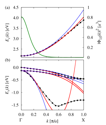
Figure 1: Fits to the band structure obtained via spin density functional theory calculations French et al. (2009) (black linespoints) for (a) conduction band and (b) valence bands of $\mathrm{Cu_{2}O}$ for the [100] direction using the expressions (7) and (8) (red lines). The green solid line shows the function $\left|\Phi_{1S}\left(\bm{k}\right)\right|^{2}$ for $a_{\mathrm{exc}}^{\left(1S\right)}=a$ in units of $a^{3}$. One can see that the differences between the fit using quartic terms and the fit of Ref. Schöne et al. (2016) (blue dashed lines) neglecting these terms are small in the range of extension of $\left|\Phi_{1S}\left(\bm{k}\right)\right|^{2}$. Note that $\left|\Phi_{1S}\!\left(\bm{k}\right)\right|^{2}$ is not shown in the lower panel for reasons of clarity.

Figure 2: Same as Fig. 1 for the [110] direction.

After replacing $H_{\mathrm{e}}\!\left(\bm{p}_{\mathrm{e}}\right)\rightarrow H_{\mathrm{e}}\!\left(\hbar\bm{k}\right)$ and $H_{\mathrm{h}}\!\left(\bm{p}_{\mathrm{h}}\right)\rightarrow-H_{\mathrm{h}}\!\left(\hbar\bm{k}\right)$, we can determine the eigenvalues of these Hamiltonians and fit them as in Ref. Schöne et al. (2016) for $\left|\bm{k}\right|<\pi/a$ to the band structure of $\mathrm{Cu_{2}O}$ obtained via spin density functional theory calculations French et al. (2009).

To obtain a reliable result, we perform a least-squares fit with a weighting function. Even though the exciton ground state will show deviations from a pure hydrogen-like $1S$ state, we expect that the radial probability density can be described qualitatively by that function. Hence, we use the modulus squared of the Fourier transform $\Phi_{1S}\!\left(\bm{k}\right)=\mathcal{F}\left(\Psi_{1S}\right)\left(\bm{k}\right)$ of the hydrogen-like function

$$\Psi_{1S}\!\left(\bm{r}\right)=\frac{1}{\sqrt{\pi\left(a_{\mathrm{exc}}^{\left(1S\right)}\right)^{3}}}e^{-r/a_{\mathrm{exc}}^{\left(1S\right)}}$$ (9)

as the weighting function for the fit. It reads Devreese and Peeters (1984)

$$\left|\Phi_{1S}\!\left(\bm{k}\right)\right|^{2} \sim \left|\frac{1}{\sqrt{(2\pi)^{3}}}\int\mathrm{d}\bm{r}\;\Psi_{1S}\!\left(\bm{r}\right)e^{-i\bm{k}\bm{r}}\right|^{2}$$ (10)

$$= \frac{8\left(a_{\mathrm{exc}}^{\left(1S\right)}\right)^{3}}{\pi^{2}\left(1+k^{2}\left(a_{\mathrm{exc}}^{\left(1S\right)}\right)^{2}\right)^{4}}$$

with the radius $a_{\mathrm{exc}}^{\left(1S\right)}$ of the $1S$ exciton state. Although we do not a priori know the true value of $a_{\mathrm{exc}}^{\left(1S\right)}$, the experimental value of the binding energy of the $1S$ state Knox (1963); Uihlein et al. (1981) as well as the calculations of Ref. Kavoulakis et al. (1997) indicate that it is on the order of one or two times the lattice constant $a=0.427\,\mathrm{nm}$ Dahl and Switzendick (1966); Elliott (1961); Kleinman and Mednick (1980). For the fit to the band structure we assume a small value of $a_{\mathrm{exc}}^{\left(1S\right)}=a$ as a lower limit in the sense of a safe estimate since then the extension of the exciton wave function in Fourier space is larger. In doing so, we will now show that even if the radius of the $1S$ exciton were smaller or equal to the lattice constant $a$, there would not be contributions of the $p^{4}$ terms of the band structure.

The results of the fit are depicted as red solid lines in Figs. 1, 2, and 3. For a comparison, we also show the fit neglecting the quartic terms in the momenta (blue dashed lines) Schöne et al. (2016). The values of the fit parameters are

$$\lambda_{1}= -1.109\times 10^{-2},\quad \lambda_{2}= -2.052\times 10^{-2},$$

$$\xi_{1}= -1.389\times 10^{-1},\quad \xi_{4}= -1.518\times 10^{-1},$$

$$\xi_{2}= \quad\>2.353\times 10^{-3},\quad \xi_{5}= \quad\>9.692\times 10^{-4},$$

$$\xi_{3}= -1.523\times 10^{-1},\quad \xi_{6}= -8.385\times 10^{-4}.$$ (11)

As can be seen, e.g., from Fig. 2, the fit including the quartic terms is only slightly better than the fit with the quadratic terms for small $k$. A clear difference between the fits can be seen only for large values of $k$ as regards the valence bands: Since some of the pre-factors of the quartic terms are positive, the energy of the valence bands in the fitted model increases for larger values of $k$.

Considering the minor differences between the fits for small $k$ and the small extension of the $1S$ exciton function in $k$ space even for $a_{\mathrm{exc}}^{\left(1S\right)}=a$ (see, e.g., Fig. 1), the quartic terms will hardly affect this exciton state and can be neglected. These arguments still hold if, e.g., $a_{\mathrm{exc}}^{\left(1S\right)}=0.2a$ is assumed.

In the work of Ref. Kavoulakis et al. (1997) the introduction of $p^{4}$ terms seemed necessary to explain the experimentally observed large mass of the $1S$ exciton. However, the experimental observations are already well described by quadratic terms in $p$ when considering the complete valence band structure Schweiner et al. (2016b). As we already stated in Ref. Schweiner et al. (2016c), a simple restriction to the $\Gamma_{7}^{+}$ band neglecting the $\Gamma_{8}^{+}$ band and considering the nonparabolicity of the $\Gamma_{7}^{+}$ band via $p^{4}$ terms as has been done in Ref. Kavoulakis et al. (1997) does not treat the problem correctly.

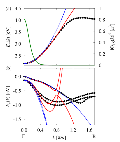
Figure 3: Same as Fig. 1 for the [111] direction.

III.2 Dielectric constant 

In the case of the $1S$ exciton in $\mathrm{Cu_{2}O}$ the relative motion of the electron and the hole is sufficiently fast that phonons cannot follow it and corrections on the dielectric constant need to be considered.

In general, the electron and the hole are coupled to longitudinal optical phonons via the Fröhlich interaction Fröhlich (1954); Toyozawa (1964) and to longitudinal acoustic phonons via the deformation potential coupling Bardeen and Shockley (1950); Toyozawa (1964). While in the case of optical phonons the ions of the solid are displaced in anti-phase and thus create a dipole moment in the unit cell of a polar crystal, the ions are displaced in phase in the case of acoustic phonons and no dipole moment is created. Hence, one expects that the interaction between electron or hole and optical phonons is much larger than the interaction with acoustic phonons in polar crystals Haken (1958); Klingshirn (2007).

If the frequency of the relative motion of electron and hole is high enough so that the ions of the solid cannot follow it, the Coulomb interaction between electron and hole is screened by the high-frequency or background dielectric constant $\varepsilon_{\mathrm{b}}$ Knox (1963); Madelung and Rössler (2001). This dielectric constant describes the electronic polarization, which can follow the motion of electron and hole very quickly Kuper and Whitefield (1963).

For lower frequencies of the relative motion the contribution of the phonons to the screening becomes important and the dielectric function $\varepsilon$ becomes frequency dependent. In many semiconductors the frequency of the relative motion in exciton states with a principal quantum number of $n\geq 2$ is so small that the low-frequency or static dielectric constant $\varepsilon_{\mathrm{s}}$ can be used Klingshirn (2007), which involves the electronic polarization and the displacement of the ions Kuper and Whitefield (1963). Note that we use the notation $\varepsilon_{\mathrm{b}}$, $\varepsilon_{\mathrm{s}}$ instead of $\varepsilon_{\infty}$, $\varepsilon_{0}$ to avoid the risk of confusion with the electric permittivity $\varepsilon_{0}$ Kuper and Whitefield (1963); Klingshirn (2007).

The transition from $-e^{2}/4\pi\varepsilon_{0}\varepsilon_{\mathrm{s}}r$ to $-e^{2}/4\pi\varepsilon_{0}\varepsilon_{\mathrm{b}}r$, which takes place when the frequency of the electron or the hole is of the same size as the frequency of the phonon Kuper and Whitefield (1963), had been investigated in detail by Haken in Refs. Haken (1956a, b, 1957, 1958); Haken and Schottky (1958); Kuper and Whitefield (1963). He considered at first the interaction between electron or hole and the phonons and then constructed the exciton from the resulting particles with polarisation clouds, i.e., the polarons. The change of the Coulomb interaction between both particles was then explained in terms of an exchange of phonons, i.e., of virtual quanta of the polarization field Kuper and Whitefield (1963).

The final result for the interaction in the transition region between $-e^{2}/4\pi\varepsilon\varepsilon_{\mathrm{s}}r$ and $-e^{2}/4\pi\varepsilon\varepsilon_{\mathrm{b}}r$ was the so-called Haken potential Haken (1956b, 1957); Haken and Schottky (1958); Knox (1963); Klingshirn (2007); Devreese and Peeters (1984),

$$V\!\left(r\right) = -\frac{e^{2}}{4\pi\varepsilon_{0}r}\left[\frac{1}{\varepsilon_{\mathrm{s}}}+\frac{1}{2\varepsilon^{*}}\left(e^{-r/\rho_{\mathrm{h}}}+e^{-r/\rho_{\mathrm{e}}}\right)\right].$$ (12)

Here $\rho_{\mathrm{e}}$ and $\rho_{\mathrm{h}}$ denote the polaron radii

$$\rho_{\mathrm{e/h}}=\sqrt{\frac{\hbar}{2m_{\mathrm{e/h}}^{*}\omega_{\mathrm{LO}}}}$$ (13)

with the frequency $\omega_{\mathrm{LO}}$ of the optical phonon and $\varepsilon^{*}$ is given by

$$\frac{1}{\varepsilon^{*}}=\frac{1}{\varepsilon_{\mathrm{b}}}-\frac{1}{\varepsilon_{\mathrm{s}}}.$$ (14)

Note that in the result of Haken Haken (1958); Menéndez-Proupin et al. (2015) the polaron masses $m_{i}^{*}$ instead of the bare electron and hole masses have to be used in the polaron radii and the kinetic energies. Furthermore, the lattice relaxation due to the interaction of excitons and phonons decreases the band gap energy for electrons and holes. However, since the value of $E_{\mathrm{g}}$ for $\mathrm{Cu_{2}O}$ has been determined in Ref. Kazimierczuk et al. (2014) from the experimental exciton spectrum, the polaron effect is already accounted for in the band gap energy Klingshirn (2007).

Note that the above results were derived in the simple band model and by assuming only one optical phonon branch contributing to the Fröhlich interaction. To the best of our knowledge there is no model accounting for more than one optical phonon branch Menéndez-Proupin et al. (2015); Kavoulakis et al. (1997); Kuper and Whitefield (1963), which complicates the correct treatment of $\mathrm{Cu_{2}O}$, where two LO phonons contribute to the Fröhlich interaction. Even though there are theories for polarons in the degenerate band case Trebin (1979); Rössler and Trebin (1981); Trebin and Rössler (1975), we will use only the leading, spherically symmetric terms, in which only the isotropic effective mass of the hole or only the Luttinger parameter $\gamma_{1}$ enters. Of course, there are further terms of cubic symmetry, which also depend on the other Luttinger parameters. However, since already $\gamma_{1}$ is at least by a factor of $2$ larger than the other Luttinger parameters, we expect the further terms in the Haken potentials to be smaller than the leading term used here. Since the effect of the Haken potential on the exciton spectrum is not crucial, as will be seen from Fig. 6, the neglection of further terms in the polaron potentials will then be a posteriori justified.

Furthermore, the Haken potential (12) cannot describe the non-Coulombic electron-hole interaction for very small values of $r$, which is due to the finite size of electron and hole Knox (1963). The conditions of validity of the potential (12) have, e.g., been discussed by Haken in Ref. Kuper and Whitefield (1963).

When treating the Haken potential numerically for different polar crystals, the experimental and theoretical binding energies of the exciton states sometimes do not agree, for which reason corrections, sometimes phenomenologically, to the Haken potential have been introduced Bajaj (1974); Pollmann and Büttner (1975); Bednarek et al. (1977); Pollmann and Büttner (1977) leading to clearly better results. One of these refined formulas is the potential proposed by Pollmann and Büttner Pollmann and Büttner (1977); Menéndez-Proupin et al. (2015)

$$V\!\left(r\right) = -\frac{e^{2}}{4\pi\varepsilon_{0}r}$$ (15)

$$\times \left[\frac{1}{\varepsilon_{\mathrm{s}}}+\frac{1}{\varepsilon^{*}}\left(\frac{m_{\mathrm{h}}}{\Delta m}e^{-r/\rho_{\mathrm{h}}}-\frac{m_{\mathrm{e}}}{\Delta m}e^{-r/\rho_{\mathrm{e}}}\right)\right],$$

in which the bare electron and hole masses have to be used and where $\Delta m$ is given by $\Delta m=m_{\mathrm{h}}-m_{\mathrm{e}}$. Hence, we take the statements given above as a reason to propose the following phenomenological potentials for $\mathrm{Cu_{2}O}$, which are motivated by the formula of Haken and by the formula of Pollmann and Büttner:

$$V^{\mathrm{H}}\!\left(r\right)=-\frac{e^{2}}{4\pi\varepsilon_{0}r}\left[\frac{1}{\varepsilon_{\mathrm{s}1}}+\frac{1}{2\varepsilon_{1}^{*}}\left(e^{-r/\rho_{\mathrm{h}1}}+e^{-r/\rho_{\mathrm{e}1}}\right)+\frac{1}{2\varepsilon_{2}^{*}}\left(e^{-r/\rho_{\mathrm{h}2}}+e^{-r/\rho_{\mathrm{e}2}}\right)\right]$$ (16a)

and

$$V^{\mathrm{PB}}\!\left(r\right) = -\frac{e^{2}}{4\pi\varepsilon_{0}r}\left[\frac{1}{\varepsilon_{\mathrm{s}1}}+\frac{1}{\varepsilon_{1}^{*}}\left(\frac{m_{0}}{m_{0}-m_{\mathrm{e}}\gamma_{1}}e^{-r/\rho_{\mathrm{h}1}}-\frac{m_{\mathrm{e}}\gamma_{1}}{m_{0}-m_{\mathrm{e}}\gamma_{1}}e^{-r/\rho_{\mathrm{e}1}}\right)\right.$$ (16b)

$$\;\,\quad\qquad\qquad+\left.\frac{1}{\varepsilon_{2}^{*}}\left(\frac{m_{0}}{m_{0}-m_{\mathrm{e}}\gamma_{1}}e^{-r/\rho_{\mathrm{h}2}}-\frac{m_{\mathrm{e}}\gamma_{1}}{m_{0}-m_{\mathrm{e}}\gamma_{1}}e^{-r/\rho_{\mathrm{e}2}}\right)\right].$$

Here we use

$$\frac{1}{\varepsilon_{i}^{*}}=\frac{1}{\varepsilon_{\mathrm{b}i}}-\frac{1}{\varepsilon_{\mathrm{s}i}}$$ (17)

and

$$\rho_{\mathrm{e}i}=\sqrt{\frac{\hbar}{2m_{\mathrm{e}}\omega_{\mathrm{LOi}}}},\qquad\rho_{\mathrm{h}i}=\sqrt{\frac{\hbar\gamma_{1}}{2m_{0}\omega_{\mathrm{LOi}}}},$$ (18)

where the energies of the phonons and the values of the dielectric constants are given by Kavoulakis et al. (1997)

$$\hbar\omega_{\mathrm{LO1}}=18.7\,\mathrm{meV},\qquad\hbar\omega_{\mathrm{LO\,2}}=87\,\mathrm{meV}$$ (19)

and

$${\varepsilon_{\mathrm{s}1}}=7.5,\qquad{\varepsilon_{\mathrm{b}1}}={\varepsilon_{\mathrm{s}2}}=7.11,\qquad{\varepsilon_{\mathrm{b}2}}=6.46.$$ (20)

As has been done in Ref. Menéndez-Proupin et al. (2015) for perovskite $\mathrm{CH_{3}NH_{3}PbI_{3}}$, we use $V_{\mathrm{H}}$ or $V_{\mathrm{PB}}$ in the Schrödinger equation without an additional fit parameter and find out which of these potentials describes the exciton spectrum of $\mathrm{Cu_{2}O}$ best. Since for the polaron radii $\rho_{\mathrm{e}}$ and $\rho_{\mathrm{h}}$ $1.6a\leq\rho\leq 4.4a$ holds, we expect the Haken or the Pollmann-Büttner potential to have a significant influence on the exciton states with $n\leq 2$.

As the Fröhlich coupling constant is small in $\mathrm{Cu_{2}O}$, i.e., it is $\alpha^{\mathrm{F}}\lesssim 0.2$ for the two optical phonons and both the electron and the hole French et al. (2009), the bare electron and hole masses differ from the polaron masses by at most 3%. Hence, we can calculate with the bare masses when using $V_{\mathrm{H}}$.

Besides the frequency dependence of the dielectric function also its momentum dependence becomes important if the exciton radius is on the order of the lattice constant. This momentum dependence of the dielectric function arises from the electronic polarization Hermanson (1966); Kavoulakis et al. (1997).

When treating the excitons of $\mathrm{Cu_{2}O}$ in momentum space, the wave functions of the $n\geq 2$ states are localized about $k=0$ so that for these states the $k$ dependence of $\varepsilon$ is not important. However, for the $1S$ state $a_{1S}\approx a$ holds and thus this state is screened by $\varepsilon$ at higher momenta $k$ Kavoulakis et al. (1997). Considering the Coulomb interaction for the $1S$ exciton in $k$ space,

$$V(k,\,\omega)=-\frac{1}{\sqrt{(2\pi)^{3}}}\,\frac{e^{2}}{\varepsilon_{0}\varepsilon(k,\,\omega)k^{2}},$$ (21)

Kavoulakis et al Kavoulakis et al. (1997) derived a correction term by assuming

$$\frac{1}{\varepsilon(k,\omega)} \approx \frac{1}{\varepsilon_{\mathrm{b}}-d(ka)^{2}}\approx\frac{1}{\varepsilon_{\mathrm{b}}}+\frac{d(ka)^{2}}{\varepsilon_{\mathrm{b}}^{2}}$$ (22)

valid for $\,E_{\mathrm{g}}/\hbar\gg\omega\gg\omega_{\mathrm{LO}}$ with a small unknown constant $d$. Inserting Eq. (22) in Eq. (21) and Fourier transforming the second expression, one obtains the following correction term to the Coulomb interaction:

$$V_{d}=-da^{2}\frac{e^{2}}{\varepsilon_{0}\varepsilon_{\mathrm{b}}^{2}}V_{\mathrm{uc}}\,\delta\!\left(\bm{r}\right)=-V_{0}V_{\mathrm{uc}}\delta\!\left(\bm{r}\right).$$ (23)

Following the calculation of Ref. Hermanson (1966) on the dielectric function and using the lowest $\Gamma_{8}^{-}$ conduction band and the highest $\Gamma_{7}^{+}$ valence band, Kavoulakis et al Kavoulakis et al. (1997) estimated the value of $d$ to $d\approx 0.18$ Kavoulakis et al. (1997).

Note that in general a Kronecker delta would appear in Eq. (23) Knox (1963). However, as we treat the exciton problem in the continuum approximation, this Kronecker delta is replaced by the delta function times the volume $V_{\mathrm{uc}}=a^{3}$ of one unit cell. Thus, the parameter $V_{0}$ has the unit of an energy.

We have already stated above that the Haken potential cannot describe the electron-hole interaction correctly for very small $r$. Therefore, we now assume that the potential (23) is not only due to the momentum dependence of the dielectric function but that it also accounts for deviations from the Haken potential at small $r$. Hence, we will treat $V_{0}$ as an unknown fit parameter in the following.

III.3 Exchange interaction 

In the Wannier equation or Hamiltonian of excitons the exchange interaction is generally not included but regarded as a correction to the hydrogen-like solution Knox (1963). Recently, we have presented a comprehensive discussion of the exchange interaction in $\mathrm{Cu_{2}O}$ Schweiner et al. (2016c). We could show, in accordance with Ref. Kavoulakis et al. (1997), that corrections to the exchange interaction due to a finite momentum $\hbar\bm{K}$ of the center of mass of the exciton are negligibly small. Hence, only the $K$ independent part of the exchange interaction Uihlein et al. (1981); Cho (1976); Rössler and Trebin (1981); Schweiner et al. (2016c)

$$H_{\mathrm{exch}}=J_{0}\left(\frac{1}{4}-\frac{1}{\hbar^{2}}\bm{S}_{\mathrm{e}}\cdot\bm{S}_{\mathrm{h}}\right)V_{\mathrm{uc}}\delta\!\left(\bm{r}\right)$$ (24)

needs to be considered. Within the simple hydrogen-like model the exchange interaction would only affect the $nS$ exciton states as these states have a nonvanishing probability density at $r=0$. However, when considering the complete valence band structure, the exciton states with even or with odd values of $L$ are coupled, and thus the exchange interaction will affect the whole even exciton series.

It is well known from experiments that the splitting between the yellow $1S$ ortho and the yellow $1S$ para exciton amounts to about $12\,\mathrm{meV}$ Kiselev and Zhilich (1972); Denisov and Makarov (1973); Pikus and Bir (1971). Hence, we have to choose the value of $\tilde{J}_{0}$ such that this splitting is reflected in the theoretical spectrum.

III.4 Summary 

Following the explanations given in Secs. III.2 and III.3, the term $V_{\mathrm{CCC}}$ in the Hamiltonian of Eq. (5) takes one of the following forms:

$$V_{\mathrm{CCC}}^{\mathrm{H}}\!\left(\bm{r}\right) = -\frac{e^{2}}{4\pi\varepsilon_{0}r}\left[\frac{1}{2\varepsilon_{1}^{*}}\left(e^{-r/\rho_{\mathrm{h}1}}+e^{-r/\rho_{\mathrm{e}1}}\right)+\frac{1}{2\varepsilon_{2}^{*}}\left(e^{-r/\rho_{\mathrm{h}2}}+e^{-r/\rho_{\mathrm{e}2}}\right)\right]$$ (25a)

$$+\left[-V_{0}+J_{0}\left(\frac{1}{4}-\frac{1}{\hbar^{2}}\bm{S}_{\mathrm{e}}\cdot\bm{S}_{\mathrm{h}}\right)\right]V_{\mathrm{uc}}\delta\!\left(\bm{r}\right),$$

$$V_{\mathrm{CCC}}^{\mathrm{PB}}\!\left(\bm{r}\right) = -\frac{e^{2}}{4\pi\varepsilon_{0}r}\left[\frac{1}{\varepsilon_{1}^{*}}\left(\frac{m_{0}}{m_{0}-m_{\mathrm{e}}\gamma_{1}}e^{-r/\rho_{\mathrm{h}1}}-\frac{m_{\mathrm{e}}\gamma_{1}}{m_{0}-m_{\mathrm{e}}\gamma_{1}}e^{-r/\rho_{\mathrm{e}1}}\right)\right.$$ (25b)

$$\;\,\quad\qquad\qquad+\left.\frac{1}{\varepsilon_{2}^{*}}\left(\frac{m_{0}}{m_{0}-m_{\mathrm{e}}\gamma_{1}}e^{-r/\rho_{\mathrm{h}2}}-\frac{m_{\mathrm{e}}\gamma_{1}}{m_{0}-m_{\mathrm{e}}\gamma_{1}}e^{-r/\rho_{\mathrm{e}2}}\right)\right]$$

$$+\left[-V_{0}+J_{0}\left(\frac{1}{4}-\frac{1}{\hbar^{2}}\bm{S}_{\mathrm{e}}\cdot\bm{S}_{\mathrm{h}}\right)\right]V_{\mathrm{uc}}\delta\!\left(\bm{r}\right),$$

[cf. Eqs. (16a), (16b), (23), and (24)]. Note that while the operators with $\delta\left(\bm{r}\right)$ affect only the exciton series with even values of $L$, the Haken or Pollmann and Büttner potential affect all exciton states Kuper and Whitefield (1963). A comparison of our results with the experimental values of Refs. Kazimierczuk et al. (2014); Uihlein et al. (1981); Thewes et al. (2015); Bloch and Schwab (1978); Heckötter (2015) will allow us, in Sec. V, to determine the size of the unknown parameters $V_{0}$ and $J_{0}$.

IV Eigenvalues and oscillator strengths 

In this section we describe how the Schrödinger equation corresponding to the Hamiltonian (5) is solved in a complete basis. Furthermore, we discuss how to calculate oscillator strengths for two-photon absorption. An appropriate basis to solve the Schrödinger equation has been presented in detail in Ref. Schweiner et al. (2016b). Hence, we recapitulate only the most important points.

As regards the angular momentum part of the basis, we have to consider that the different operators in the Hamiltonian couple the quasi spin $I$, the hole spin $S_{\mathrm{h}}$, and the angular momentum $L$ of the exciton. Hence, we introduce the effective hole spin $J=I+S_{\mathrm{h}}$, the angular momentum $F=L+J$, and the total angular momentum $F_{t}=F+S_{\mathrm{e}}$. For the radial part of the exciton wave function we use the Coulomb-Sturmian functions Caprio et al. (2012)

$$U_{NL}\!\left(r\right)=N_{NL}^{(\alpha)}\left(2\rho\right)^{L}e^{-\rho}L_{N}^{2L+1}\left(2\rho\right)$$ (26)

with $\rho=r/\alpha$, an arbitrary convergence or scaling parameter $\alpha$, the associated Laguerre polynomials $L_{n}^{m}\left(x\right)$, and a normalization factor

$$N_{NL}^{(\alpha)}=\frac{2}{\sqrt{\alpha^{3}}}\left[\frac{N!}{\left(N+L+1\right)\left(N+2L+1\right)!}\right]^{\frac{1}{2}}.$$ (27)

The radial quantum number $N$ is related to the principal quantum number $n$ via $n=N+L+1$. Finally, we use the following ansatz for the exciton wave function

$$\left|\Psi\right\rangle = \sum_{NLJFF_{t}M_{F_{t}}}c_{NLJFF_{t}M_{F_{t}}}\left|\Pi\right\rangle,$$ (28a)

$$\left|\Pi\right\rangle = \left|N,\,L;\,\left(I,\,S_{\mathrm{h}}\right)\,J;\,F,\,S_{\mathrm{e}};\,F_{t},\,M_{F_{t}}\right\rangle$$ (28b)

with real coefficients $c$. The parenthesis and semicolons in Eq. (28b) are meant to illustrate the coupling scheme of the spins and the angular momenta. Since the $z$ axis is a fourfold axis, it is sufficient to use only $M_{F_{t}}$ quantum numbers which differ by $\pm 4$ in Eq. (28).

We now express the Hamiltonian (5) in terms of irreducible tensors Edmonds (1960); Baldereschi and Lipari (1973); Broeckx (1991). Inserting the ansatz (28) in the Schrödinger equation $H\Psi=E\Psi$ and multiplying from the left with another basis state $\left\langle\Pi^{\prime}\right|$, we obtain a matrix representation of the Schrödinger equation of the form

$$\bm{D}\bm{c}=E\bm{M}\bm{c}.$$ (29)

The vector $\bm{c}$ contains the coefficients of the ansatz (28). All matrix elements, which enter the symmetric matrices $\bm{D}$ and $\bm{M}$ and which have not been treated in Ref. Schweiner et al. (2016b), are given in Appendix D. The generalized eigenvalue problem (29) is finally solved using an appropriate LAPACK routine Anderson et al. (1999). The material parameters used in our calculation are listed in Table 1.

Since the basis cannot be infinitely large, the values of the quantum numbers are chosen in the following way: For each value of $n=N+L+1$ we use

$$L = 0,\,\ldots,\,n-1,$$

$$J = 1/2,\,3/2,$$

$$F = \left|L-J\right|,\,\ldots,\,\min\left(L+J,\,F_{\mathrm{max}}\right),$$ (30)

$$F_{t} = F-1/2,\,F+1/2,$$

$$M_{F_{t}} = -F_{t},\,\ldots,\,F_{t}.$$

The value $F_{\mathrm{max}}$ and the maximum value of $n$ are chosen appropriately large so that the eigenvalues converge. Additionally, we can use the scaling parameter $\alpha$ to enhance convergence. However, it should be noted that the value of $\alpha$ does not influence the theoretical results for the exciton energies in any way, i.e., the converged results do not depend on the value of $\alpha$.

Table 1: Material parameters used in the calculations. Instead of the band gap energy $E_{\mathrm{g}}=2.17208\,\mathrm{eV}$ of Ref. Kazimierczuk et al. (2014) a slightly smaller value is used to obtain a better agreement with experimental values in Sec. V.

band gap energy	$E_{\mathrm{g}}=2.17202\,\mathrm{eV}$
electron mass	$m_{\mathrm{e}}=0.99\,m_{0}$	Hodby et al. (1976)
spin-orbit coupling	$\Delta=0.131\,\mathrm{eV}$	Schöne et al. (2016)
valence band parameters	$\gamma_{1}=1.76$	Schöne et al. (2016); Schweiner et al. (2016b)
	$\gamma_{2}=0.7532$	Schöne et al. (2016); Schweiner et al. (2016b)
	$\gamma_{3}=-0.3668$	Schöne et al. (2016); Schweiner et al. (2016b)
	$\eta_{1}=-0.020$	Schöne et al. (2016); Schweiner et al. (2016b)
	$\eta_{2}=-0.0037$	Schöne et al. (2016); Schweiner et al. (2016b)
	$\eta_{3}=-0.0337$	Schöne et al. (2016); Schweiner et al. (2016b)
lattice constant	$a=0.42696\,\mathrm{nm}$	Swanson and Fuyat (1953)
dielectric constants	$\varepsilon_{\mathrm{s}1}=7.5$	Madelung and Rössler (2001)
	$\varepsilon_{\mathrm{b}1}=\varepsilon_{\mathrm{s}2}=7.11$	Madelung and Rössler (2001)
	$\varepsilon_{\mathrm{b}2}=6.46$	Madelung and Rössler (2001)
energy of $\Gamma_{4}^{-}$-LO phonons	$\hbar\omega_{\mathrm{LO1}}=18.7\,\mathrm{meV}$	Kavoulakis et al. (1997)
	$\hbar\omega_{\mathrm{LO2}}=87\,\mathrm{meV}$	Kavoulakis et al. (1997)

Note that the presence of the delta functions in Eq. (25) makes the whole problem more complicated than in Ref. Schweiner et al. (2016b) since not only the eigenvalues but also the wave functions at $r=0$ have to converge. However, for a specific value of $\alpha$ it is not possible to obtain convergence for all exciton states of interest. Therefore, we solve the Schrödinger equation initially without the $\delta\!\left(\bm{r}\right)$ dependent terms. We then select the converged eigenvectors and with these we set up a second generalized eigenvalue problem now including the $\delta\!\left(\bm{r}\right)$ dependent terms. This problem is again solved using an appropriate LAPACK routine Anderson et al. (1999) and provides the correct converged eigenvalues of the complete Hamiltonian (5).

Having solved the eigenvalue problem, we can use the eigenvectors to determine relative oscillator strengths. The determination of relative oscillator strengths in one-photon absorption has been presented in detail in Refs. Schweiner et al. (2016b, 2017b). While in one photon absorption excitons of symmetry $\Gamma_{4}^{-}$ are dipole-allowed Schweiner et al. (2016b), the selection rules for two-photon absorption Inoue and Toyozawa (1965); Bader and Gold (1968); Denisov and Makarov (1972) are different and excitons of symmetry $\Gamma_{5}^{+}$ can be optically excited.

When considering one-photon absorption one generally treats the operator $\bm{A}\bm{p}$ with the vector potential $\bm{A}$ of the radiation field in first order perturbation theory. The dipole operator then transforms according to the irreducible representation $D^{1}$ of the full rotation group. In two-photon absorption one needs the operator $\bm{A}\bm{p}$ twice and thus the product $D^{1}\otimes D^{1}=D^{0}\oplus D^{1}\oplus D^{2}$ has to be considered Koster et al. (1963). In $\mathrm{Cu_{2}O}$ the reduction of these irreducible representations by the cubic group $O_{\mathrm{h}}$ has to be considered and one obtains

$$\Gamma_{4}^{-}\otimes\Gamma_{4}^{-}=\Gamma_{1}^{+}\oplus\Gamma_{4}^{+}\oplus\left(\Gamma_{3}^{+}\oplus\Gamma_{5}^{+}\right).$$ (31)

In two-photon absorption the spin $S=S_{\mathrm{e}}+S_{\mathrm{h}}=0$ remains unchanged and the exciton state must have an $L=0$ component. Hence, the correct expression for the relative oscillator strength is given by

$$f_{\mathrm{rel}}\sim\left|\lim_{r\rightarrow 0}\,{}_{T}\left\langle 1,\,M^{\prime}_{F_{t}}\middle|\Psi\left(\bm{r}\right)\right\rangle\right|^{2},$$ (32)

with the wave function $\left|\Psi\right\rangle$ of Eq. (28) and the state $\left|F^{\prime}_{t},\,M^{\prime}_{F_{t}}\right\rangle_{T}$, which is a short notation for

$$\left|\left(S_{\mathrm{e}},\,S_{\mathrm{h}}\right)\,S,\,I;\,I+S,\,L;\,F^{\prime}_{t},\,M^{\prime}_{F_{t}}\right\rangle$$ (33)

$$= \left|\left(1/2,\,1/2\right)\,0,\,1;\,1,\,0;\,F^{\prime}_{t},\,M^{\prime}_{F_{t}}\right\rangle.$$

Note that the coupling scheme of the spins and angular momenta in Eq. (33) given by

$$S_{\mathrm{e}}+S_{\mathrm{h}}=S\quad\rightarrow\quad(I+S)+L=F^{\prime}_{t}$$ (34)

is different from the one of Eq. (28b) due to the requirement that $S$ must be a good quantum number.

It can be shown that the state $\left|1,\,M^{\prime}_{F_{t}}\right\rangle_{T}$ transforms according to the irreducible representation $\Gamma_{5}^{+}$ of $O_{\mathrm{h}}$ Koster et al. (1963), for which reason only exciton states of this symmetry can be excited in two-photon absorption. By choosing particular directions of the polarization of the light, e.g., by choosing one photon being polarized in $x$ direction and one photon being polarized in $y$ direction, only one component of the $\Gamma_{5}^{+}$ exciton states, the $xy$ component, can be excited optically. We consider this case in the following and hence use $M^{\prime}_{F_{t}}=0$ in Eq. (32). Finally, we wish to note that the exciton states of symmetry $\Gamma_{5}^{+}$ can weakly be observed in one-photon absorption in quadrupole approximation Uihlein et al. (1981).

V Results and discussion 

In this section we determine the values of the parameters $J_{0}$ and $V_{0}$ and discuss the complete exciton spectrum of $\mathrm{Cu_{2}O}$.

The parameter $J_{0}$ describes the strength of the exchange interaction. It is well known that the exchange interaction mainly affects the $1S$ exciton and that the splitting between the ortho and the para exciton state amounts to $11.8\,\mathrm{meV}$ Kiselev and Zhilich (1972); Denisov and Makarov (1973); Pikus and Bir (1971); Uihlein et al. (1981); Bloch and Schwab (1978). By choosing

$$J_{0}=0.792\pm 0.068\,\mathrm{eV}$$ (35)

we obtain the correct value of this splitting irrespective of whether using the Haken or the Pollman-Büttner potential [cf. Eq. (25)].

The figures 4 and 5 show the effect of the correction with the coefficient $V_{0}$ on the spectrum for the Haken and the Pollman-Büttner potential, respectivley. As can be seen from these figures, the exchange splitting of the $1S$ state hardly changes when varying the value $V_{0}$. Hence, we can determine $V_{0}$ almost independently of $J_{0}$.

To find the optimum value of $V_{0}$, we compare our results to the energies of the even parity exciton states given in Refs. Uihlein et al. (1981); Schöne et al. (2016); Heckötter et al. (2017); Heckötter (2015); Bloch and Schwab (1978); an Yu. A. Stepanov (1975). However, we can see from Figs. 4 and 5 that there is no value of $V_{0}$ for which all theoretical results take the values of the experimentally determined energies. This is not unexpected since the central-cell corrections are only an attempt to account for the specific properties of the $1S$ exciton within the continuum limit of Wannier excitons and are not an exact description of this exciton state. Hence, we do not expect a perfect agreement between theory and experiment.

Small deviations from the experimental values could also be explained by small uncertainties in the Luttinger parameters $\gamma_{i}$, $\eta_{i}$ Schöne et al. (2016); Schweiner et al. (2016b) or the band gap energy Kazimierczuk et al. (2014) as well as by a finite temperature or small strains in the crystal. On the other hand, it is also possible that the experimental values are affected by uncertainties. This can be seen, e.g., when comparing the slightly different experimental results of Refs. Schöne et al. (2016) and Heckötter et al. (2017); Heckötter (2015).

Note that the almost perfect agreement between theoretical and experimental results in Refs. Fröhlich et al. (1979); Uihlein et al. (1981) could only be obtained by taking also $\gamma_{1}^{\prime}$, $\mu^{\prime}$ and $\Delta$ as fit parameters to the experiment. However, these parameters are connected to the band structure in $\mathrm{Cu_{2}O}$ French et al. (2009) and cannot be chosen arbitrarily Thewes et al. (2015); Schweiner et al. (2016b).

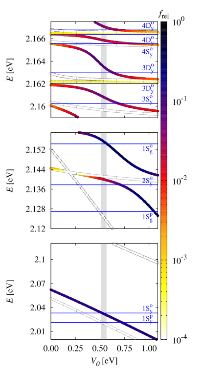
Figure 4: Behavior of the even exciton states as functions of $V_{0}$ when using $V_{\mathrm{CCC}}^{\mathrm{H}}$ [see Eq. (25a)]. The color bar shows the relative oscillator strengths for two-photon absorption. The blue straight lines denote the position of the dipole-allowed $\Gamma_{5}^{+}$ $S$ and $D$ exciton states observed in the experiment. We also show the positions of the $1S$ para excitons $(1S_{\mathrm{y/g}}^{\mathrm{p}})$. The gray area indicates the optimum range of $V_{0}=0.539\pm\,0.027\,\mathrm{eV}$, where the ratio of the relative oscillator strengths of the yellow $2S$ and the green $1S$ state amounts to $\sim 16$. The effect of the central-cell corrections on the whole even exciton spectrum is evident. For further information see text.

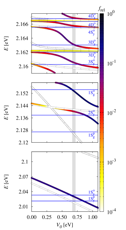
Figure 5: Same calculation as in Fig. 4 but with $V_{\mathrm{CCC}}^{\mathrm{PB}}$ [see Eq. (25b)]. One can see only slight differences for the $n=1$ and $n=2$ exciton states when comparing the results to Fig. 4. The gray area indicates the optimum range of $V_{0}=0.694\pm\,0.027\,\mathrm{eV}$.

Table 2: Decomposition of the irreducible representations of the rotation group or the angular momentum states by the cubic group $O_{\mathrm{h}}$. Note that the quasi-spin $I$ already enters the momentum $F$ via $J$. The irreducible representations denote the symmetry of the envelope function $\left(L\right)$, the combined symmetry of envelope and hole $\left(F\right)$ or the complete symmetry of the exciton $\left(F_{t}\right)$.

$L$		$F=L+J\,\left(J=\frac{1}{2}\right)$		$F_{t}=F+S_{\mathrm{e}}$
$0$	$\Gamma_{1}^{+}$	$\frac{1}{2}$	$\Gamma_{7}^{+}$	$0$	$\Gamma_{2}^{+}$
				$1$	$\Gamma_{5}^{+}$
$1$	$\Gamma_{4}^{-}$	$\frac{1}{2}$	$\Gamma_{7}^{-}$	$0$	$\Gamma_{2}^{-}$
				$1$	$\Gamma_{5}^{-}$
		$\frac{3}{2}$	$\Gamma_{8}^{-}$	$1$	$\Gamma_{4}^{-}$
				$2$	$\Gamma_{3}^{-}\oplus\Gamma_{5}^{-}$
$2$	$\Gamma_{3}^{+}\oplus\Gamma_{5}^{+}$	$\frac{3}{2}$	$\Gamma_{8}^{+}$	$1$	$\Gamma_{5}^{+}$
				$2$	$\Gamma_{3}^{+}\oplus\Gamma_{4}^{+}$
		$\frac{5}{2}$	$\Gamma_{6}^{+}\oplus\Gamma_{8}^{+}$	$2$	$\Gamma_{3}^{+}\oplus\Gamma_{4}^{+}$
				$3$	$\Gamma_{1}^{+}\oplus\Gamma_{4}^{+}\oplus\Gamma_{5}^{+}$
$3$	$\Gamma_{2}^{-}\oplus\Gamma_{4}^{-}\oplus\Gamma_{5}^{-}$	$\frac{5}{2}$	$\Gamma_{6}^{-}\oplus\Gamma_{8}^{-}$	$2$	$\Gamma_{3}^{-}\oplus\Gamma_{4}^{-}$
				$3$	$\Gamma_{1}^{-}\oplus\Gamma_{4}^{-}\oplus\Gamma_{5}^{-}$
		$\frac{7}{2}$	$\Gamma_{6}^{-}\oplus\Gamma_{7}^{-}\oplus\Gamma_{8}^{-}$	$3$	$\Gamma_{1}^{-}\oplus\Gamma_{4}^{-}\oplus\Gamma_{5}^{-}$
				$4$	$\Gamma_{2}^{-}\oplus\Gamma_{3}^{-}\oplus\Gamma_{4}^{-}\oplus\Gamma_{5}^{-}$
$L$		$F=L+J\,\left(J=\frac{3}{2}\right)$		$F_{t}=F+S_{\mathrm{e}}$
$0$	$\Gamma_{1}^{+}$	$\frac{3}{2}$	$\Gamma_{8}^{+}$	$1$	$\Gamma_{5}^{+}$
				$2$	$\Gamma_{3}^{+}\oplus\Gamma_{4}^{+}$

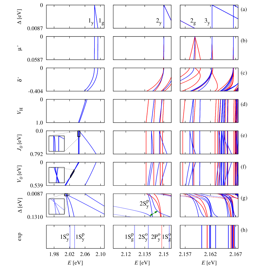
Figure 6: Exciton spectrum of the even (blue) and odd (red) exciton states when increasing all material parameters from zero (top) to their correct values (bottom) and using $V_{\mathrm{CCC}}^{\mathrm{H}}$ [cf. Eq. (25b)]. If all material parameters except for $\gamma_{1}^{\prime}$ are set to zero, one obtains a hydrogen-like spectrum, for which the yellow (y) and green (g) exciton states are degenerate [$\Delta=0$ in (a)]. When increasing the spin-orbit coupling constant $\Delta$, this degeneracy is lifted and the green exciton states are shifted towards higher energies (a). Note that we increase $\Delta$ in two steps to its true value of $\Delta=0.131\,\mathrm{eV}$ for reasons of clarity. One can then follow these states from (b) to (g). Since the effect of the parameters $\eta_{1}^{\prime}$, $\nu$ and $\tau$ on the exciton spectrum is small they are immediately set from zero to their correct values between (c) and (d). In (g) and (h) the para and ortho exciton states are denoted by an upper index p and o. The final results at the bottom of (g), which are also listed in Table 3, can then be compared to the position of the exciton states obtained from experiments (h). Note that due to the marked anticrossing [green arrow in the second panel of (g)] the assignment of the green $1S$ state and the yellow $2S$ state changes.

Table 3: Comparison of calculated energies $E_{\mathrm{theor}}$ to experimental values $E_{\mathrm{exp}}$ (References given behind experimental values) when using the central-cell corrections with the Haken potential (25a). The even exciton states are listed in blue text and the odd exciton states in red text. Note that we use $E_{\mathrm{g}}=2.17202\,\mathrm{eV}$ instead of $E_{\mathrm{g}}=2.17208\,\mathrm{eV}$ Kazimierczuk et al. (2014) to obtain a better agreement. The assignment of the states in the first column is motivated by Fig. 6 but is generally not instructive due to the large deviations from the hydrogen-like model. Hence, we also give the symmetry of the states. In the case of the $P$ and $F$ excitons we do not give the symmetry of the complete exciton state but only the combined symmetry of envelope and hole. As regards the $5G$ excitons we only give the average energy of the states of symmetry $\Gamma_{5}^{+}$. The value in the fourth column gives the relative oscillator strength in one-photon absorption ($nP$, $nF$ excitons; see Ref. Schweiner et al. (2016b)) or in two-photon absorption ($nS$, $nD$, $nG$ excitons; see Eq. (32)). Note that due to the interaction with the $1S_{\mathrm{g}}$ state the oscillator strength of the $2S_{\mathrm{y}}$ state is much smaller than expected when assuming two independent, i.e., green and yellow, series. The value in the last column indicates the percentage of the $J=3/2$ component of the state, i.e., the green part. Note that due to the interaction between the yellow and the green exciton series the green $1S$ state is spread over several yellow exciton states. The green states with $n\geq 2$ are located far above the states listed here.

State			$E_{\mathrm{exp}}$ [eV]	$E_{\mathrm{theor}}$ [eV]	$f_{\mathrm{rel}}$	gp [%]			State			$E_{\mathrm{exp}}$ [eV]	$E_{\mathrm{theor}}$ [eV]	$f_{\mathrm{rel}}$	gp [%]
$1S_{\mathrm{y}}$	$\Gamma_{2}^{+}$		$2.0212$ Bloch and Schwab (1978)	2.0200	–	5.49			$4D_{\mathrm{y}}$	$\Gamma_{3/4}^{+}$		$2.16629$ Heckötter et al. (2017); Heckötter (2015)	2.16644	–	0.19
$1S_{\mathrm{y}}$	$\Gamma_{5}^{+}$		$2.0330$ Uihlein et al. (1981)	2.0320	26.60	7.22			$4D_{\mathrm{y}}$	$\Gamma_{5}^{+}$		$2.16638$ Heckötter et al. (2017); Heckötter (2015)	2.16645	0.07	0.19
									$4D_{\mathrm{y}}$	$\Gamma_{1/4}^{+}$		–	2.16646	–	0.16
$1S_{\mathrm{g}}$	$\Gamma_{3/4}^{+}$		$2.1269$ an Yu. A. Stepanov (1975)	2.1245	–	71.62			$4F_{\mathrm{y}}$	$\Gamma_{7}^{-}$		–	2.16653	–	0.12
									$4F_{\mathrm{y}}$	$\Gamma_{8}^{-}$		$2.16652$ Thewes et al. (2015)	2.16654	0.066	0.10
$2S_{\mathrm{y}}$	$\Gamma_{5}^{+}$		$2.1378$ Uihlein et al. (1981)	2.1399	3.55	10.88			$4F_{\mathrm{y}}$	$\Gamma_{8}^{-}$		$2.16654$ Thewes et al. (2015)	2.16656	0.002	0.08
$2S_{\mathrm{y}}$	$\Gamma_{2}^{+}$		–	2.1412	–	1.43			$4F_{\mathrm{y}}$	$\Gamma_{6}^{-}$		$2.16654$ Thewes et al. (2015)	2.16657	0.010	0.08
$2P_{\mathrm{y}}$	$\Gamma_{8}^{-}$		$2.1484$ Kazimierczuk et al. (2014)	2.1475	351.4	1.91			$4F_{\mathrm{y}}$	$\Gamma_{6}^{-}$		$2.16658$ Thewes et al. (2015)	2.16660	0.011	0.06
$2P_{\mathrm{y}}$	$\Gamma_{7}^{-}$		–	2.1480	–	1.30			$4D_{\mathrm{y}}$	$\Gamma_{3/4}^{+}$		–	2.16658	–	0.22
									$4D_{\mathrm{y}}$	$\Gamma_{5}^{+}$		$2.16677$ Heckötter et al. (2017); Heckötter (2015)	2.16704	6.86	3.67
$1S_{\mathrm{g}}$	$\Gamma_{5}^{+}$		$2.1544$ Uihlein et al. (1981)	2.1553	56.01	36.88
									$5S_{\mathrm{y}}$	$\Gamma_{2}^{+}$		–	2.16798	–	0.10
$3S_{\mathrm{y}}$	$\Gamma_{2}^{+}$		–	2.15967	–	0.48			$5S_{\mathrm{y}}$	$\Gamma_{5}^{+}$		$2.16801$ Heckötter et al. (2017); Heckötter (2015)	2.16816	2.02	0.81
$3S_{\mathrm{y}}$	$\Gamma_{5}^{+}$		$2.16027$ Heckötter et al. (2017); Heckötter (2015)	2.16080	10.34	4.49			$5P_{\mathrm{y}}$	$\Gamma_{8}^{-}$		$2.16829$ Kazimierczuk et al. (2014)	2.16825	32.82	0.25
$3P_{\mathrm{y}}$	$\Gamma_{8}^{-}$		$2.16135$ Kazimierczuk et al. (2014)	2.16119	147.3	0.93			$5P_{\mathrm{y}}$	$\Gamma_{7}^{-}$		–	2.16830	–	0.18
$3P_{\mathrm{y}}$	$\Gamma_{7}^{-}$		–	2.16141	–	0.63			$5D_{\mathrm{y}}$	$\Gamma_{3/4}^{+}$		$2.16841$ Heckötter et al. (2017); Heckötter (2015)	2.16846	–	0.11
$3D_{\mathrm{y}}$	$\Gamma_{3/4}^{+}$		$2.16183$ Heckötter et al. (2017); Heckötter (2015)	2.16213	–	0.31			$5D_{\mathrm{y}}$	$\Gamma_{5}^{+}$		$2.16846$ Heckötter et al. (2017); Heckötter (2015)	2.16846	0.05	0.12
$3D_{\mathrm{y}}$	$\Gamma_{5}^{+}$		$2.16202$ Heckötter et al. (2017); Heckötter (2015)	2.16215	0.09	0.30			$5D_{\mathrm{y}}$	$\Gamma_{1/4}^{+}$		–	2.16847	–	0.10
$3D_{\mathrm{y}}$	$\Gamma_{1/4}^{+}$		–	2.16217	–	0.25			$5F_{\mathrm{y}}$	$\Gamma_{7}^{-}$		–	2.16850	–	0.09
$3D_{\mathrm{y}}$	$\Gamma_{3/4}^{+}$		–	2.16237	–	0.46			$5F_{\mathrm{y}}$	$\Gamma_{8}^{-}$		$2.16851$ Thewes et al. (2015)	2.16850	0.069	0.07
$3D_{\mathrm{y}}$	$\Gamma_{5}^{+}$		$2.16303$ Heckötter et al. (2017); Heckötter (2015)	2.16348	15.04	8.49			$5F_{\mathrm{y}}$	$\Gamma_{8}^{-}$		$2.16852$ Thewes et al. (2015)	2.16852	0.000	0.06
									$5F_{\mathrm{y}}$	$\Gamma_{6}^{-}$		$2.16852$ Thewes et al. (2015)	2.16852	0.002	0.06
$4S_{\mathrm{y}}$	$\Gamma_{2}^{+}$		–	2.16547	–	0.21			$5F_{\mathrm{y}}$	$\Gamma_{6}^{-}$		$2.16855$ Thewes et al. (2015)	2.16855	0.001	0.04
$4S_{\mathrm{y}}$	$\Gamma_{5}^{+}$		$2.16555$ Heckötter et al. (2017); Heckötter (2015)	2.16584	3.79	1.53			$5D_{\mathrm{y}}$	$\Gamma_{3/4}^{+}$		–	2.16854	–	0.11
$4P_{\mathrm{y}}$	$\Gamma_{8}^{-}$		$2.16609$ Kazimierczuk et al. (2014)	2.16604	67.43	0.45			$5\bar{G}_{\mathrm{y}}$	$\Gamma_{5}^{+}$		–	2.16855	0.00	0.03
$4P_{\mathrm{y}}$	$\Gamma_{7}^{-}$		–	2.16614	–	0.32			$5D_{\mathrm{y}}$	$\Gamma_{5}^{+}$		$2.16860$ Heckötter et al. (2017); Heckötter (2015)	2.16879	4.30	2.22

Table 4: Same comparison as in Table 3 but when using the central-cell corrections with the Pollmann-Büttner potential (25b). Especially for the states with $n<3$ differences in the calculated energies can be observed when using the different corrections (25a) or (25b). Note that for each $n$ the relative oscillator strength of one $nD$ state is larger than the relative oscillator strengths of the $nS$ state in accordance with the experimental results of Ref. Uihlein et al. (1981).

State			$E_{\mathrm{exp}}$ [eV]	$E_{\mathrm{theor}}$ [eV]	$f_{\mathrm{rel}}$	gp [%]			State			$E_{\mathrm{exp}}$ [eV]	$E_{\mathrm{theor}}$ [eV]	$f_{\mathrm{rel}}$	gp [%]
$1S_{\mathrm{y}}$	$\Gamma_{2}^{+}$		$2.0212$ Bloch and Schwab (1978)	2.0180	–	5.49			$4D_{\mathrm{y}}$	$\Gamma_{3/4}^{+}$		$2.16629$ Heckötter et al. (2017); Heckötter (2015)	2.16646	–	0.17
$1S_{\mathrm{y}}$	$\Gamma_{5}^{+}$		$2.0330$ Uihlein et al. (1981)	2.0300	27.90	6.83			$4D_{\mathrm{y}}$	$\Gamma_{5}^{+}$		$2.16638$ Heckötter et al. (2017); Heckötter (2015)	2.16647	0.53	0.18
									$4D_{\mathrm{y}}$	$\Gamma_{1/4}^{+}$		–	2.16648	–	0.15
$1S_{\mathrm{g}}$	$\Gamma_{3/4}^{+}$		$2.1269$ an Yu. A. Stepanov (1975)	2.1254	–	65.53			$4F_{\mathrm{y}}$	$\Gamma_{7}^{-}$		–	2.16653	–	0.12
									$4F_{\mathrm{y}}$	$\Gamma_{8}^{-}$		$2.16652$ Thewes et al. (2015)	2.16654	0.078	0.10
$2S_{\mathrm{y}}$	$\Gamma_{5}^{+}$		$2.1378$ Uihlein et al. (1981)	2.1401	4.22	11.16			$4F_{\mathrm{y}}$	$\Gamma_{8}^{-}$		$2.16654$ Thewes et al. (2015)	2.16657	0.002	0.08
$2S_{\mathrm{y}}$	$\Gamma_{2}^{+}$		–	2.1414	–	1.31			$4F_{\mathrm{y}}$	$\Gamma_{6}^{-}$		$2.16654$ Thewes et al. (2015)	2.16657	0.009	0.08
$2P_{\mathrm{y}}$	$\Gamma_{8}^{-}$		$2.1484$ Kazimierczuk et al. (2014)	2.1482	292.3	1.72			$4F_{\mathrm{y}}$	$\Gamma_{6}^{-}$		$2.16658$ Thewes et al. (2015)	2.16660	0.010	0.05
$2P_{\mathrm{y}}$	$\Gamma_{7}^{-}$		–	2.1486	–	1.20			$4D_{\mathrm{y}}$	$\Gamma_{3/4}^{+}$		–	2.16661	–	0.19
									$4D_{\mathrm{y}}$	$\Gamma_{5}^{+}$		$2.16677$ Heckötter et al. (2017); Heckötter (2015)	2.16686	3.24	1.82
$1S_{\mathrm{g}}$	$\Gamma_{5}^{+}$		$2.1544$ Uihlein et al. (1981)	2.1535	65.25	42.41
									$5S_{\mathrm{y}}$	$\Gamma_{2}^{+}$		–	2.16800	–	0.09
$3S_{\mathrm{y}}$	$\Gamma_{2}^{+}$		–	2.15974	–	0.44			$5S_{\mathrm{y}}$	$\Gamma_{5}^{+}$		$2.16801$ Heckötter et al. (2017); Heckötter (2015)	2.16811	1.17	0.48
$3S_{\mathrm{y}}$	$\Gamma_{5}^{+}$		$2.16027$ Heckötter et al. (2017); Heckötter (2015)	2.16053	7.83	3.29			$5P_{\mathrm{y}}$	$\Gamma_{8}^{-}$		$2.16829$ Kazimierczuk et al. (2014)	2.16829	28.17	0.24
$3P_{\mathrm{y}}$	$\Gamma_{8}^{-}$		$2.16135$ Kazimierczuk et al. (2014)	2.16138	125.9	0.86			$5P_{\mathrm{y}}$	$\Gamma_{7}^{-}$		–	2.16834	–	0.17
$3P_{\mathrm{y}}$	$\Gamma_{7}^{-}$		–	2.16158	–	0.60			$5D_{\mathrm{y}}$	$\Gamma_{3/4}^{+}$		$2.16841$ Heckötter et al. (2017); Heckötter (2015)	2.16847	–	0.10
$3D_{\mathrm{y}}$	$\Gamma_{3/4}^{+}$		$2.16183$ Heckötter et al. (2017); Heckötter (2015)	2.16217	–	0.28			$5D_{\mathrm{y}}$	$\Gamma_{5}^{+}$		$2.16846$ Heckötter et al. (2017); Heckötter (2015)	2.16847	0.04	0.12
$3D_{\mathrm{y}}$	$\Gamma_{5}^{+}$		$2.16202$ Heckötter et al. (2017); Heckötter (2015)	2.16219	0.07	0.29			$5D_{\mathrm{y}}$	$\Gamma_{1/4}^{+}$		–	2.16848	–	0.09
$3D_{\mathrm{y}}$	$\Gamma_{1/4}^{+}$		–	2.16221	–	0.24			$5F_{\mathrm{y}}$	$\Gamma_{7}^{-}$		–	2.16850	–	0.09
$3D_{\mathrm{y}}$	$\Gamma_{3/4}^{+}$		–	2.16243	–	0.41			$5F_{\mathrm{y}}$	$\Gamma_{8}^{-}$		$2.16851$ Thewes et al. (2015)	2.16851	0.078	0.07
$3D_{\mathrm{y}}$	$\Gamma_{5}^{+}$		$2.16303$ Heckötter et al. (2017); Heckötter (2015)	2.16308	8.42	4.87			$5F_{\mathrm{y}}$	$\Gamma_{8}^{-}$		$2.16852$ Thewes et al. (2015)	2.16852	0.000	0.06
									$5F_{\mathrm{y}}$	$\Gamma_{6}^{-}$		$2.16852$ Thewes et al. (2015)	2.16853	0.001	0.06
$4S_{\mathrm{y}}$	$\Gamma_{2}^{+}$		–	2.16550	–	0.19			$5F_{\mathrm{y}}$	$\Gamma_{6}^{-}$		$2.16855$ Thewes et al. (2015)	2.16855	0.001	0.04
$4S_{\mathrm{y}}$	$\Gamma_{5}^{+}$		$2.16555$ Heckötter et al. (2017); Heckötter (2015)	2.16575	2.45	0.98			$5D_{\mathrm{y}}$	$\Gamma_{3/4}^{+}$		–	2.16855	0.00	0.03
$4P_{\mathrm{y}}$	$\Gamma_{8}^{-}$		$2.16609$ Kazimierczuk et al. (2014)	2.16612	58.29	0.43			$5\bar{G}_{\mathrm{y}}$	$\Gamma_{5}^{+}$		–	2.16856	–	0.07
$4P_{\mathrm{y}}$	$\Gamma_{7}^{-}$		–	2.16621	–	0.31			$5D_{\mathrm{y}}$	$\Gamma_{5}^{+}$		$2.16860$ Heckötter et al. (2017); Heckötter (2015)	2.16868	1.68	0.92

It can be seen from Figs. 4 and 5 that the oscillator strength of the exciton state at $E\approx 2.143\,\mathrm{eV}$ changes rapidly with increasing $V_{0}$. From the experimental results of Refs. Fröhlich et al. (1979); Uihlein et al. (1981) we know that the two exciton states at $E=2.1378\,\mathrm{eV}$ and $E=2.1544\,\mathrm{eV}$ are well separated from the other exciton states and that the phonon background is small. Hence, the ratio of the relative two-photon oscillator strengths can be calculated quite accurately to $\sim\!16$.

We now choose the value of $V_{0}$ such that the ratio of the calculated two-photon oscillator strengths reaches the same value and obtain

$$V_{0}=0.539\pm\,0.027\,\mathrm{eV}$$ (36)

when using the Haken potential [cf. Eq. (25a)] or

$$V_{0}=0.694\pm\,0.027\,\mathrm{eV}$$ (37)

when using the Pollmann-Büttner potential [cf. Eq. (25b)]. Note that the error bars for $V_{0}$ are chosen such that the ratio of the oscillator strengths lies between $14$ and $18$.

Having determined the most suitable values of $V_{0}$ and $J_{0}$, we can now turn our attention to the exciton Bohr radius $a_{\mathrm{exc}}^{\left(1S\right)}$ of the $1S$ ortho exciton and to the correct assignment of the $n=2$ exciton states.

To determine the radius $a_{\mathrm{exc}}^{\left(1S\right)}$, we evaluate

$$\left\langle\Psi\middle|r\middle|\Psi\right\rangle = \sum_{N^{\prime}}\sum_{NLJFF_{t}M_{F_{t}}}c_{N^{\prime}LJFF_{t}M_{F_{t}}}c_{NLJFF_{t}M_{F_{t}}}$$ (38)

$$\times \sum_{j=-2}^{2}\frac{\alpha\left(R_{2}\right)^{j}_{NL}}{N+L+j+1}\delta_{N^{\prime},\,N+j}$$

with the wave function $\Psi$ of Eq. (28) and compare the result with the formula Gallagher (1988)

$$\left\langle r\right\rangle=\frac{1}{2}a_{\mathrm{exc}}\left[3n^{2}-L\left(L+1\right)\right]$$ (39)

known from the hydrogen atom, where we set $n=1$ and $L=0$. Note that the function $\left(R_{2}\right)^{j}_{NL}$ in Eq. (38) is taken from the recursion relations of the Coulomb-Sturmian functions in the Appendix of Ref. Schweiner et al. (2016b). We obtain

$$a_{\mathrm{exc}}^{\left(1S\right)}\approx 0.793\,\mathrm{nm}\approx 1.86\,a$$ (40)

when using the Haken potential or

$$a_{\mathrm{exc}}^{\left(1S\right)}\approx 0.810\,\mathrm{nm}\approx 1.90\,a$$ (41)

when using the Pollmann-Büttner potential. In both cases the radius of the $1S$ ortho exciton is large enough that the corrections to the kinetic energy discussed in Sec. III.1 can certainly be neglected.

Let us now proceed to the correct assignment of the $n=2$ exciton states. Since in the investigation of Uihlein et al Fröhlich et al. (1979); Uihlein et al. (1981) the wrong values for the Luttinger parameters were used (cf. Ref. Schweiner et al. (2016b)), it is not clear whether the state at $E=2.1544\,\mathrm{eV}$ can still be assigned as the yellow $2S$ ortho exciton state and the state at $E=2.1378\,\mathrm{eV}$ as the green $1S$ ortho exciton state when using the correct Luttinger parameters.

To demonstrate from which hydrogen-like states the experimentally observed exciton states originate, we find it instructive to start from the hydrogen-like spectrum with almost all material parameters set to zero and then increase these material parameters successively to their true values. This is shown in Fig. 6.

At first all material parameters except for $\gamma_{1}^{\prime}$ are set to zero, so that a true hydrogen-like spectrum is obtained, where the yellow (y) and green (g) exciton states are degenerate. This spectrum is shown in the panel (a) of Fig. 6. When increasing the spin-orbit coupling constant $\Delta$ in Fig. 6(a), the degeneracy between the green and the yellow exciton series is lifted. The increase of the Luttinger parameters $\mu^{\prime}$ and $\delta^{\prime}$ in the panels (b) and (c) furthermore lifts the degeneracy between the exciton states of different angular momentum $L$. The Haken potential does not change degeneracies but slightly lowers the energy of the exciton states in Fig. 6(d). The exchange energy described by the constant $J_{0}$ lifts the degenercy between ortho and para exciton states in Fig. 6(e). As the operator $\delta\!\left(\bm{r}\right)$ affects only the states of even parity (blue lines), the energy of the odd exciton states (red lines) remains unchanged in Fig. 6(f). Note that we increase $\Delta$ in two steps to its true value of $\Delta=0.131\,\mathrm{eV}$ for reasons of clarity. Hence, at the bottom of Fig. 6(g) all material values have been increased to their true values. For a comparison, we show in panel (h) the position of the experimentally observed states. Following the exciton states from panel (a) to (g), it is possible to assign them with the notation $nL^{\mathrm{p/o}}_{\mathrm{y/g}}$, where the upper index denotes a para or an ortho exciton state and the lower index a yellow or a green state.

The results presented in Fig. 6 suggest to assign the exciton state at $E=2.1378\,\mathrm{eV}$ to the green $1S$ ortho exciton state. However, one can observe an anticrossing between the green $1S$ state and the yellow $2S$ state, which is indicated by a green arrow in Fig. 6(g). Hence, the assignment has to be changed. As a proof, we can calculate the percentage of the $J=3/2$ component of these states, i.e., their green part, by evaluating

$$\mathrm{gp}=\left\langle\Psi\middle|P\middle|\Psi\right\rangle$$ (42)

with the projection operator

$$P=\sum_{M_{J}=-3/2}^{3/2}\left|\frac{3}{2},\,M_{J}\right\rangle\left\langle\frac{3}{2},\,M_{J}\right|$$ (43)

and the exciton wave function $\left|\Psi\right\rangle$ (see also Appendix C).

The green part gp of the state at $E\approx 2.1544\,\mathrm{eV}$ is distinctly higher ($\mathrm{gp}\approx 40\%$) than the green part of the exciton state at $E\approx 2.1378\,\mathrm{eV}$ ($\mathrm{gp}\approx 11\%$). However, since also $\mathrm{gp}\approx 40\%$ is significantly smaller than one, we see that the assignment of this exciton state as the ground state of the green series is questionable and shows the significant deviations from the hydrogen-like model. The green $1S$ exciton state is distributed over the yellow states. Note that in Ref. Uihlein et al. (1981) also the state of higher energy had a larger green part than the state of lower energy. However, in Fig. 2 of Ref. Uihlein et al. (1981) the assignment is reversed since the limit of $\mu^{\prime}\rightarrow 0$ was used to designate the states. It seems obvious that a similar anticrossing between the green $1S$ state and the yellow $2S$ state was disregarded. A considerable effect of the interaction between the green and yellow series is the change in the oscillator strength of the states. The oscillator strength of the $2S_{y}$ state is much smaller than expected when assuming two independent, i.e., green and yellow, series Fröhlich et al. (1979); Uihlein et al. (1981) (cf. also Tables 3 and 4).

For reasons of completeness, we give the size of the green $1S$ and the yellow $2S$ state by evaluating Eq. (38). Since these states are strongly mixed and a correct assignment with a principal quantum number $n$ is not possible, we do not use the formula (39). We obtain

$$\left\langle r\right\rangle\left(2S_{y}\right) \approx 4.32\,\mathrm{nm}\approx 10.1\,a,$$ (44a)

$$\left\langle r\right\rangle\left(1S_{g}\right) \approx 5.32\,\mathrm{nm}\approx 12.5\,a,$$ (44b)

when using the Haken potential or

$$\left\langle r\right\rangle\left(2S_{y}\right) \approx 4.39\,\mathrm{nm}\approx 10.3\,a,$$ (45a)

$$\left\langle r\right\rangle\left(1S_{g}\right) \approx 4.09\,\mathrm{nm}\approx 9.58\,a,$$ (45b)

when using the Pollmann-Büttner potential. We see that in both cases the values of $\left\langle r\right\rangle$ for the green $1S$ and the yellow $2S$ state are of the same size. This is expected due to the strong mixing of both states.

The resonance of the green $1S$ state with the yellow exciton series and the mixing of all even exciton states via the cubic band structure leads to an admixture of $D$ and $G$ states to the green $1S$ state. Hence, the three $\Gamma_{5}^{+}$ states which we assigned with $1S_{\mathrm{g}}$ are elliptically deformed and invariant only under the subgroup $D_{4\mathrm{h}}$ of $O_{\mathrm{h}}$ Schweiner et al. (2016b); Koster et al. (1963). The lower symmetry of the envelope function allows for a smaller mean distance between electron and hole in a specific direction, which leads to a gain of energy due to the Coulomb interaction Schweiner et al. (2016b). As regards the $xy$-component, the symmetry axis of the according subgroup $D_{4\mathrm{h}}$ is the $z$-axis of the crystal. Since for this state the expectation values $\left\langle\Psi\middle|x^{2}\middle|\Psi\right\rangle$ and $\left\langle\Psi\middle|y^{2}\middle|\Psi\right\rangle$ are identical, we can calculate the semi-principal axes of the elliptically deformed state by evaluating

$$\left\langle\Psi\middle|x^{2}\middle|\Psi\right\rangle = \left\langle\Psi\middle|\frac{1}{2}\left(r^{2}-z^{2}\right)\middle|\Psi\right\rangle$$ (46)

$$= \sum_{N^{\prime}L^{\prime}J^{\prime}F^{\prime}F_{t}^{\prime}M_{F_{t}}^{\prime}}\sum_{NLJFF_{t}M_{F_{t}}}$$

$$c_{N^{\prime}L^{\prime}J^{\prime}F^{\prime}F_{t}^{\prime}M_{F_{t}}^{\prime}}c_{NLJFF_{t}M_{F_{t}}}$$

$$\times \alpha^{2}\left\langle\Pi^{\prime}\middle|\frac{1}{3}r^{2}-\frac{1}{3\sqrt{6}}X^{(2)}_{0}\middle|\Pi\right\rangle$$

and

$$\left\langle\Psi\middle|z^{2}\middle|\Psi\right\rangle = \sum_{N^{\prime}L^{\prime}J^{\prime}F^{\prime}F_{t}^{\prime}M_{F_{t}}^{\prime}}\sum_{NLJFF_{t}M_{F_{t}}}$$ (47)

$$c_{N^{\prime}L^{\prime}J^{\prime}F^{\prime}F_{t}^{\prime}M_{F_{t}}^{\prime}}c_{NLJFF_{t}M_{F_{t}}}$$

$$\times \alpha^{2}\left\langle\Pi^{\prime}\middle|\frac{1}{3}\sqrt{\frac{2}{3}}X^{(2)}_{0}+\frac{1}{3}r^{2}\middle|\Pi\right\rangle$$

with the wave function $\Psi$ of Eq. (28) and the matrix elements $\langle\Pi^{\prime}|X^{(2)}_{0}|\Pi\rangle$ and $\langle\Pi^{\prime}|r^{2}|\Pi\rangle$ listed in the Appendix of Ref. Schweiner et al. (2017b). We obtain

$$\left\langle x^{2}\right\rangle \approx 116.4\,a^{2},$$

$$\left\langle z^{2}\right\rangle \approx 29.9\,a^{2},$$ (48)

when using the Haken potential or

$$\left\langle x^{2}\right\rangle \approx 68.6\,a^{2},$$

$$\left\langle z^{2}\right\rangle \approx 25.1\,a^{2},$$ (49)

when using the Pollmann-Büttner potential. The significant differences in $\left\langle x^{2}\right\rangle$ and $\left\langle z^{2}\right\rangle$ show again the strong resonance of the green $1S$ state with the yellow series as well as the strong admixture of states with $L\geq 2$. We finally want to note that, due to the coupling of the yellow and green series, the green $1S$ has to be regarded as an excited state in the complete exciton spectrum and not as the ground state of the green series. In particular, the green $1S$ state is orthogonal to the true ground state of the complete spectrum, i.e., to the yellow $1S$ state.

Let us now discuss the other exciton states. To determine the number of para and ortho exciton states as well as their degeneracies for the different values of $L$, one can use group theoretical considerations. In the spherical approximation, in which the cubic part of the Hamiltonian is neglected $\left(\delta^{\prime}=0\right)$, the momentum $F=J+L$ is a good quantum number for the states of negative parity since the exchange interaction does not act on these states. The states of positive parity can be classified by the total momentum $F_{t}=F+S_{\mathrm{e}}$ in the spherical approximation.

If the complete cubic Hamiltonian is treated, the reduction of the irreducible representations $D^{F}$ or $D^{F_{t}}$ of the rotation group by the cubic group $O_{\mathrm{h}}$ has to be considered Abragam and Bleaney (1970). This is shown in Table 2. As has already been stated in Ref. Schweiner et al. (2016b), a normal spin one transforms according to the irreducible representation $\Gamma_{4}^{+}$ of the cubic group whereas the quasi-spin $I$ transforms according to $\Gamma_{5}^{+}=\Gamma_{4}^{+}\otimes\Gamma_{2}^{+}$. Therefore, one has to include the additional factor $\Gamma_{2}^{+}$ when determining the symmetry of an exciton state Uihlein et al. (1981); Thewes et al. (2015); Schweiner et al. (2016b). This symmetry is given by the symmetry of the envelope function, the valence band, and the conduction band:

$$\Gamma_{\mathrm{exc}}=\Gamma_{\mathrm{env}}\otimes\Gamma_{\mathrm{v}}\otimes\Gamma_{\mathrm{c}}.$$ (50)

Only states of symmetry $\Gamma_{4}^{-}$ are dipole allowed in one-photon absorption and only states of symmetry $\Gamma_{5}^{+}$ are dipole allowed in two-photon absorption. Hence, we see from Table 2 that there are at the most one $P$ state and four $F$ states or one $S$ and two $D$ states for each principal quantum number $n$, which can be observed in experiments.

Since the exchange interaction does not act on the exciton states with negative parity, one can use the irreducible representations of the second column of Table 2 to classify these exciton states Thewes et al. (2015). For the exciton states of positive parity the irreducible representations of the third column are needed. Note that the cubic part of the Hamiltonian mixes the $S$ and $D$ exciton states of symmetry $\Gamma_{5}^{+}$. Hence, the exchange interaction acts only on the $D$ excitons of symmetry $\Gamma_{5}^{+}$ via their $S$ component. The degeneracies between the $D$ states of symmetry $\Gamma_{3}^{+}$ and $\Gamma_{4}^{+}$ or $\Gamma_{1}^{+}$ and $\Gamma_{4}^{+}$ is not lifted, respectively (cf. the third column of Table 2).

Since neither $J$ nor $F$ are good quantum numbers due to the cubic symmetry of our Hamiltonian, we do not use the nomenclature $n^{2J+1}L_{F}$ of Refs. Fröhlich et al. (1979); Uihlein et al. (1981). Although $L$ is likewise no good quantum number, the assignment of the exciton states by using $S$, $P$, $D$, $F$ and $G$ to denote the angular momentum is still common (see, e.g., Refs. Schöne et al. (2016); Thewes et al. (2015)). Hence, we feel obliged to classify the states by introducing the notation $nL_{\mathrm{y}/\mathrm{g}}$ for comparison with other works but also stress that this is generally not instructive due to the large deviations from the hydrogen-like model (cf. also Ref. Schweiner et al. (2016b)). By the index y or g we denote the yellow or the green exciton series, respectively. To be more correct, we will also give the symmetry of the exciton states in terms of the irreducible representations of Table 2. These symmetries can be determined by regarding the eigenvectors of the generalized eigenvalue problem (29) Schweiner et al. (2016b).

In the Tables 3 and 4 we now give a direct comparison between experimental and theoretical exciton energies for all states with $n\leq 5$. One can see that the results with the Haken potential listed in Tab. 3 show a better agreement with the experimental values than the results with the Pollmann-Büttner potential listed in Tab. 4. Hence, we have chosen the central-cell corrections with the Haken potential for the calculation of Fig. 6.

The Haken potential or the Pollmann-Büttner potential also slightly affects the odd exciton series and especially the $2P$ exciton state. These potentials shift the energy of the $\Gamma_{4}^{-}$ (resp. $\Gamma_{8}^{-}$) $2P$ exciton state by an amount of $210\,\mathrm{\upmu eV}$ (Haken) or $880\,\mathrm{\upmu eV}$ (Pollmann-Büttner) towards lower energies.

VI Summary and outlook 

We have treated the exciton spectrum of $\mathrm{Cu_{2}O}$ considering the complete valence band structure, the exchange interaction, and the central-cell corrections. A thorough discussion of the central-cell corrections revealed that only the frequency and momentum dependence of the dielectric function $\varepsilon\left(k,\,\omega\right)$ have to be accounted for. Due to the estimated size of the $1S$ exciton Bohr radius, corrections to the kinetic energy can be neglected. Hence, only the two parameters $V_{0}$ and $J_{0}$ are decisive for the relative position of the exciton states. While $J_{0}$ describes the splitting of the exciton states into ortho and para components, $V_{0}$ changes the relative energy of the states but leaves this splitting between ortho and para component of the same exciton state almost unchanged. Hence, these parameters could be determined almost independently. This means that our results are not very sensitive to the choice of the parameters used. Instead, there is only one combination of both parameters $J_{0}$ and $V_{0}$ given in Eqs. (35)-(37), for which our results are in good agreement with the experiment.

We have shown that the central-cell corrections considerably affect the complete even exciton series since the valence band structure couples the $1S$ state to higher exciton states. The frequency dependence of the dielectric function also slightly affects the odd exciton series and lowers, in particular, the energy of the $2P$ exciton state. Furthermore, we have demonstrated that due to the coupling of the yellow and the green exciton series the green $1S$ exciton state is distributed over all yellow states.

In contrast to earlier works Heckötter et al. (2017), we have presented a closed theory of the complete exciton series in $\mathrm{Cu_{2}O}$, where we explicitly give the correction potentials (25a) or (25b). Hence, the introduction of quantum defects or the introduction of different exchange parameters for different exciton states, which take the effect of the central cell corrections into account only phenomenologically, is redundant Heckötter et al. (2017); Schöne et al. (2016).

The results of our theory show a very good agreement with experimental values (see Table. 3). Therefore, we are confident that an according extension of our theory will allow for the calculation of exciton spectra in $\mathrm{Cu_{2}O}$ in electric or in combined electric and magnetic fields.

Appendix A $p^{4}$-Terms

As has already been stated in Sec. III.1, the terms of the fourth power of $\bm{p}$ span a fifteen dimensional space with the basis functions

$$p_{i}^{4},\quad p_{i}^{3}p_{j},\quad p_{i}^{2}p_{j}^{2},\quad p_{i}p_{j}p_{k}^{2}$$ (51)

with $i,j,k\in\{1,2,3\}$ and $i\neq j\neq k\neq i$. The six linear combinations of $p^{4}$ terms (including the quasi spin $I$), which transform according to $\Gamma_{1}^{+}$ Koster et al. (1963) read in terms of irreducible tensors

$$\mathrm{(I):}\quad p^{4},$$ (52a)

$$\mathrm{(II):}\quad P^{(4)}\left(\Gamma_{1}^{+}\right),$$ (52b)

$$\mathrm{(III):}\quad p^{2}\left(P^{(2)}\cdot I^{(2)}\right),$$ (52c)

$$\mathrm{(IV):}\quad p^{2}\left[P^{(2)}\times I^{(2)}\right]^{(4)}\left(\Gamma_{1}^{+}\right),$$ (52d)

$$\mathrm{(V):}\quad \left[P^{(4)}\times I^{(2)}\right]^{(4)}\left(\Gamma_{1}^{+}\right),$$ (52e)

$$\mathrm{(VI):}\quad \left[P^{(4)}\times I^{(2)}\right]^{(6)}\left(\Gamma_{1}^{+}\right),$$ (52f)

with

$$T^{(4)}\left(\Gamma_{1}^{+}\right)=\sqrt{\frac{5}{24}}\sum_{k=\pm 4}T^{(4)}_{k}+\sqrt{\frac{7}{12}}T^{(4)}_{0},$$ (53a)

and

$$T^{(6)}\left(\Gamma_{1}^{+}\right)=-\frac{\sqrt{7}}{4}\sum_{k=\pm 4}T^{(6)}_{k}+\frac{1}{\sqrt{8}}T^{(6)}_{0}.$$ (53b)

One can choose appropriate linear combinations of the states (I)-(VI):

$$\frac{1}{5}\mathrm{(I)}-\frac{1}{3\sqrt{30}}\mathrm{(II)}= \>\left[p_{1}^{2}p_{2}^{2}+\mathrm{c.p.}\right]$$ (54a)

$$\frac{2}{3}\hbar^{2}\mathrm{(I)}+\frac{2}{45}\mathrm{(III)}+\frac{1}{18}\sqrt{\frac{24}{5}}\mathrm{(IV)}= \>\bm{p}^{2}\left[p_{1}^{2}\bm{I}_{1}^{2}+\mathrm{c.p.}\right]$$ (54b)

$$\frac{1}{30}\mathrm{(III)}-\frac{1}{36}\sqrt{\frac{24}{5}}\mathrm{(IV)}= \>\bm{p}^{2}\left[p_{1}p_{2}\left\{\bm{I}_{1},\,\bm{I}_{2}\right\}+\mathrm{c.p.}\right]$$ (54c)

$$\frac{6}{5}\hbar^{2}\mathrm{(I)}-\frac{8}{9\sqrt{30}}\hbar^{2}\mathrm{(II)}-\frac{4}{27}\sqrt{\frac{7}{11}}\mathrm{(V)}+\frac{1}{9}\sqrt{\frac{14}{33}}\mathrm{(VI)}= \>\left[\left(p_{1}^{4}+6p_{2}^{2}p_{3}^{2}\right)\bm{I}_{1}^{2}+\mathrm{c.p.}\right]$$ (54d)

$$-\frac{1}{18}\sqrt{\frac{7}{11}}\mathrm{(V)}-\frac{1}{9}\sqrt{\frac{14}{33}}\mathrm{(IV)}= \>\left[\left(p_{1}^{2}+p_{2}^{2}-6p_{3}^{2}\right)p_{1}p_{2}\left\{\bm{I}_{1},\,\bm{I}_{2}\right\}+\mathrm{c.p.}\right]$$ (54e)

with $\left\{a,b\right\}=\frac{1}{2}\left(ab+ba\right)$ and c.p. denoting cyclic permutation. These linear combinations enter the generalized expressions of the kinetic energy of the hole and the electron in Sec. III.1.

Appendix B Oscillator strengths

We now give the formula for the expression

$$\lim_{r\rightarrow 0}\,{}_{T}\left\langle 1,\,M^{\prime}_{F_{t}}\middle|\Psi\left(\bm{r}\right)\right\rangle,$$ (55)

which is needed for the evaluation of the relative oscillator strength $f_{\mathrm{rel}}$ (32) in two photon absorption experiments. Using the wave function of Eq. (28), we find

$$\>\lim_{r\rightarrow 0}\,{}_{T}\left\langle 1,\,M^{\prime}_{F_{t}}\middle|\Psi\left(\bm{r}\right)\right\rangle$$

$$= \>\sum_{NFF_{t}}\sum_{M_{S_{\mathrm{e}}}}c_{N0FFF_{t}M^{\prime}_{F_{t}}}\;\sqrt{\frac{2}{\alpha^{3}}}$$

$$\times \>\left(-1\right)^{F-2M_{S_{\mathrm{e}}}+\frac{1}{2}}\left[(2F+1)(2F_{t}+1)\right]^{\frac{1}{2}}$$

$$\times \>\left(\begin{array}[]{ccc}F&\frac{1}{2}&F_{t}\\ M^{\prime}_{F_{t}}-M_{S_{\mathrm{e}}}&M_{S_{\mathrm{e}}}&-M^{\prime}_{F_{t}}\end{array}\right)$$ (58)

$$\times \>\left(\begin{array}[]{ccc}1&\frac{1}{2}&F\\ M^{\prime}_{F_{t}}&-M_{S_{\mathrm{e}}}&M_{S_{\mathrm{e}}}-M^{\prime}_{F_{t}}\end{array}\right).$$ (61)

Appendix C Green part of $\Psi$

Here we give the formula for the scalar product which is needed to calculate the green part of the wave function $\Psi$ as

$$\mathrm{gp}=\sum_{M_{J}=-3/2}^{3/2}\left\langle\Psi\middle|\frac{3}{2},\,M_{J}\right\rangle\left\langle\frac{3}{2},\,M_{J}\middle|\Psi\right\rangle.$$ (62)

We find

$$\>\left\langle\Psi\middle|\frac{3}{2},\,M_{J}\right\rangle\left\langle\frac{3}{2},\,M_{J}\middle|\Psi\right\rangle$$

$$= \>\sum_{j=-1}^{1}\sum_{NLFF_{t}M_{F_{t}}}\sum_{F^{\prime}F_{t}^{\prime}M_{F_{t}}^{\prime}}\sum_{M_{S_{\mathrm{e}}}M_{L}}\frac{\left(R_{1}\right)_{NL}^{j}}{N+L+j+1}$$

$$\times \>c_{(N+j)LJF^{\prime}F_{t}^{\prime}M_{F_{t}}^{\prime}}c_{NLJFF_{t}M_{F_{t}}}$$

$$\times \>\left(-1\right)^{F+F^{\prime}+M_{F_{t}}+M_{F_{t}}^{\prime}-2J+2M_{J}-1}$$

$$\times \>\left[(2F+1)(2F_{t}+1)(2F^{\prime}+1)(2F_{t}^{\prime}+1)\right]^{\frac{1}{2}}$$

$$\times \>\left(\begin{array}[]{ccc}F&\frac{1}{2}&F_{t}\\ M_{L}+M_{J}&M_{S_{\mathrm{e}}}&-M_{F_{t}}\end{array}\right)$$ (65)

$$\times \>\left(\begin{array}[]{ccc}L&J&F\\ M_{L}&M_{J}&-M_{L}-M_{J}\end{array}\right)$$ (68)

$$\times \>\left(\begin{array}[]{ccc}F^{\prime}&\frac{1}{2}&F_{t}^{\prime}\\ M_{L}+M_{J}&M_{S_{\mathrm{e}}}&-M_{F_{t}}^{\prime}\end{array}\right)$$ (71)

$$\times \>\left(\begin{array}[]{ccc}L&J&F^{\prime}\\ M_{L}&M_{J}&-M_{L}-M_{J}\end{array}\right).$$ (74)

The function $\left(R_{1}\right)_{NL}^{j}$ is taken from the recursion relations of the Coulomb-Sturmian functions in the Appendix of Ref. Schweiner et al. (2016b).

Appendix D Matrix elements

In this section we give the matrix elements of the terms in Eq. (25) in the basis of Eq. (28b) in Hartree units. The normalization factor $N_{NL}^{\left(\alpha\right)}$ is given in Eq. (27). All other matrix elements, which enter the symmetric matrices $\bm{D}$ and $\bm{M}$ in Eq. (29) and which are not given here, are listed in the Appendix of Ref. Schweiner et al. (2016b).

$$\left\langle\Pi^{\prime}\left|\delta\left(\bm{r}\right)\right|\Pi\right\rangle= \>\delta_{L^{\prime}0}\delta_{L0}\delta_{JJ^{\prime}}\delta_{F_{t}F^{\prime}_{t}}\delta_{M_{F_{t}}M^{\prime}_{F_{t}}}\>\frac{1}{\pi}\left(-1\right)^{F_{t}+F^{\prime}+F+J+\frac{1}{2}}$$

$$\times \>\left[\left(2F_{t}+1\right)\left(2F+1\right)\left(2F^{\prime}+1\right)\right]^{\frac{1}{2}}\left\{\begin{array}[]{ccc}F^{\prime}&F_{t}&\frac{1}{2}\\ F_{t}&F&0\end{array}\right\}\left\{\begin{array}[]{ccc}0&F^{\prime}&J\\ F&0&0\end{array}\right\},$$ (79)

$$\left\langle\Pi^{\prime}\left|\bm{S}_{\mathrm{e}}\cdot\bm{S}_{\mathrm{h}}\,\delta\left(\bm{r}\right)\right|\Pi\right\rangle= \>\delta_{L^{\prime}0}\delta_{L0}\delta_{F_{t}F^{\prime}_{t}}\delta_{M_{F_{t}}M^{\prime}_{F_{t}}}\>\frac{3}{2\pi}\left(-1\right)^{F_{t}+F^{\prime}+F+J+J^{\prime}}$$

$$\times \>\left[\left(2F+1\right)\left(2F^{\prime}+1\right)\left(2J+1\right)\left(2J^{\prime}+1\right)\right]^{\frac{1}{2}}$$

$$\times \>\left\{\begin{array}[]{ccc}F^{\prime}&F&1\\ \frac{1}{2}&\frac{1}{2}&F_{t}\end{array}\right\}\left\{\begin{array}[]{ccc}F&F^{\prime}&1\\ J^{\prime}&J&0\end{array}\right\}\left\{\begin{array}[]{ccc}\frac{1}{2}&J^{\prime}&1\\ J&\frac{1}{2}&1\end{array}\right\},$$ (86)

$$\left\langle\Pi^{\prime}\left|\frac{1}{r}e^{-r/\rho}\right|\Pi\right\rangle= \>\delta_{LL^{\prime}}\delta_{JJ^{\prime}}\delta_{F_{t}F_{t}^{\prime}}\delta_{M_{F_{t}}M_{F_{t}}^{\prime}}\>\frac{1}{4}N_{N^{\prime}L}^{\left(1\right)}N_{NL}^{\left(1\right)}\>\sum_{k=0}^{N^{\prime}}\>\sum_{j=0}^{N}\left(-1\right)^{k+j}$$

$$\times \>\binom{N^{\prime}+2L+1}{N^{\prime}-k}\binom{N+2L+1}{N-j}\frac{\left(2L+k+j+1\right)!}{k!\,j!}\left[\frac{2\rho}{1+2\rho}\right]^{\left(2+2L+k+j\right)}.$$ (87)

References

- Knox (1963) R. Knox, Theory of excitons, edited by H. Ehrenreich, F. Seitz, and D. Turnbull, Solid State Physics Supplement, Vol. 5 (Academic, New York, 1963).