We present an asymptotically flat, spherically symmetric, static, globally regular and horizonless solution of SU$(2)$-gauged $\mathcal{N}=1,d=5$ supergravity. The SU$(2)$ gauge field is that of the BPST instanton. We argue that this solution, analogous to the global monopoles found in $d=4$ $\mathcal{N}=2$ and $\mathcal{N}=4$ gauged supergravities, describes the field of a single string-theory object which does not contribute to the entropy of black holes when we add it to them and show that it is, indeed, the dimensional reduction on T⁵ of the gauge 5-brane. We investigate how the energy of the solution is concentrated as a function of the instanton’s scale showing that it never violates the hoop conjecture although the curvature grows unboundedly in the zero scale limit.

Introduction

Fueled by the research on theories of elementary particles and fundamental fields (Yang-Mills, Kaluza-Klein, Supergravity, Superstrings…), over the last 30 years, the search for and study of solutions of theories of gravity coupled to fundamental matter fields (scalars and vectors in $d=4$ and higher-rank differential forms in higher dimensions) has been enormously successful and it has revolutionized our knowledge of gravity itself. Each new classical solution to the Einstein equations (vacua, black holes, cosmic strings, domain walls, black rings, black branes, multi-center solutions…) sheds new light on different aspects of gravity and, often, on the underlying fundamental theories. For instance, although the string effective field theories (supergravities, typically) only describe the massless modes of string theory, it is possible to learn much through them about the massive non-perturbative states of the fundamental theory because they appear as classical solutions of the effective theories. Beyond this, there is a definite program in the quest to construct horizonless microstate geometries as classical solutions of Supergravity theories [4, 5]. When interpreted within the context of the fuzzball conjecture [6], these geometries have been proposed to correspond to the classical description of black hole microstates. Therefore, in the best case scenario, it might be possible to find a large collection ($\sim e^{S}$) of microstate geometries with the same asymptotic charges as a particular black hole, and, furthermore, to identify explicitly their role in the ensemble of black-hole microstates. See Refs. [7, 8] for recent progress in that direction.

Apart from the fact that they describe gravity, one of the most interesting features of string theories is that their spectra include non-Abelian Yang-Mills (YM) gauge fields. This aspect is crucial for their use in BSM phenomenology but has often been neglected in the search for classical solutions of their effective field theories, specially in lower dimensions, which have been mostly focused on theories with Abelian vector fields and with, at most, an Abelian gauging. Thus, the space of extremal (supersymmetric and non-supersymmetric, spherically-symmetric and multi-center) black-hole solutions of 4- and 5-dimensional ungauged supergravities has been exhaustively explored and progress has been made in the Abelian gauged case, motivated by the AdS/CFT correspondence, but the non-Abelian case has drawn much less attention in the string community and, correspondingly, there are just a few solutions of the string effective action (and of supergravity theories in general) with non-Abelian fields in the literature.

One of the main reasons for that is the intrinsic difficulty of solving the highly non-linear equations of motion. This difficulty, however, has not prevented the General Relativity community from attacking the problem in simpler theories such as the Einstein-Yang-Mills (EYM) or Einstein-Yang-Mills-Higgs (EYMH) theories, although it has prevented them from finding analytical solutions: most of the genuinely non-Abelian solutions are known only numerically. Another reason is that non-Abelian YM solutions are much more difficult to understand than the Abelian ones (specially when they are known only numerically): in the Abelian case we can characterize the electromagnetic field of a black hole, say, by its electric and magnetic charge, dipoles and higher multipoles. In the non-Abelian case the fields are usually characterized by topological invariants or constructions such as t’ Hooft’s magnetic monopole charge.

In general, the systems studied by the GR community (the EYM or EYMH theories in particular) are not part of any theory with extended local supersymmetry (a $\mathcal{N}>1$ supergravity with more than 4 supercharges) and, therefore, the use of supersymmetric solution-generating techniques is not possible. One can, however, consider the minimal $\mathcal{N}>1$ supergravity theories that include non-Abelian YM fields, which are amenable to those methods. Some time ago we started the search for supersymmetric solution-generating methods in $\mathcal{N}=2,d=4$ [13] and $\mathcal{N}=1,d=5$ [14, 15, 16, 17] Super-Einstein-Yang-Mills (SEYM) theories. The results obtained have allowed to construct, for the first time (at least in fully analytical form), several interesting supersymmetric solutions with genuine non-Abelian hair: global monopoles and extremal static black holes in 4 [18, 19, 20] and 5 dimensions [20], rotating black holes and black rings in 5 dimensions [21], non-Abelian 2-center solutions in 4 dimensions [19] and the first non-Abelian microstate geometries [22].

Many of the black-hole solutions found by these methods can be embedded in string theory and, in that framework, one can try to address the microscopic interpretation of their entropy, which seems to have relevant contributions from the non-Abelian fields, even though, typically, they decay so fast at infinity that they do not seem to contribute to the mass. Following the pioneer’s route [23, 24] requires an understanding of the stringy objects (D-branes etc.) that contribute to the 4- and 5-dimensional solutions’ charges. Furthermore, the interpretation of the non-Abelian microstate geometries would benefit from the knowledge of their stringy origin. In this paper, as a previous step towards the microscopic interpretation of the 5-dimensional non-Abelian black holes’ entropy which we will undertake in a forthcoming publication [25], we identify the elementary component of the simplest, static, spherically symmetric, non-Abelian 5-dimensional black hole that carries all the non-Abelian hair. The solution that describes this component turns out to be asymptotically flat, globally regular, and horizonless and the non-Abelian field is that of a BPST instanton [26] living in constant-time hypersurfaces. Only a few solutions supported by elementary fields with these characteristics are known analytically: the global monopoles found in gauged $\mathcal{N}=4,d=4$ supergravity [27, 28, 29] and also in $\mathcal{N}=2,d=4$ SEYM theories [13, 19] whose non-Abelian field is that of a BPS ’t Hooft-Polyakov monopole.

The simplest string embedding of this solution is in the Heterotic Superstring and the 10-dimensional solution whose dimensional reduction over $T^{5}$ gives this 5-dimensional global instanton turns out to be the gauge 5-brane found in Ref. [30]. This is, therefore, the non-Abelian ingredient present in the non-Abelian 5-dimensional black holes and rings constructed in Refs. [20, 21].

In what follows, we are going to derive the global instanton solution as a component of the 5-dimensional non-Abelian black holes, we show that it is the Heterotic String gauge 5-brane compactified on $T^{5}$ and we study the dependence of the distribution of energy on the instanton’s scale parameter, showing that, no matter how small it is, there is never more energy concentrated in a 3-sphere of radius $R$ than that of a Schwarzschild-Tangerlini black hole of radius $R$.

1 The global instanton solution

We are going to work in the context of the ST$[2,6]$ model of $\mathcal{N}=1,d=5$ supergravity (which is a model with 5 vector supermultiplets) with an SU$(2)$ gauging in the $I=3,4,5$ sector. This theory is briefly described in Appendix A and the solution-generating technique that allows us to construct timelike supersymmetric solutions of this theory with one isometry is explained in Appendix B.

Our goal is to construct the minimal non-singular solution that includes in the SU$(2)$ sector the following solution of the Bogomol’nyi equations

$$\Phi^{A}=\frac{1}{g_{4}r(1+\lambda^{2}r)}\frac{x^{A}}{r}\,,\hskip 28.45274pt\breve{A}^{A}{}_{B}=\varepsilon^{A}{}_{BC}\frac{1}{g_{4}r(1+\lambda^{2}r)}\frac{x^{C}}{r}\,.\hskip 28.45274ptr^{2}\equiv x^{s}x^{s}\,,$$ (1.1)

This solution describes a coloured monopole [18, 20], one of the singular solutions found by Protogenov [31]. Observe that this solution is written in terms of the 4($=1+3$)-dimensional Yang-Mills coupling constant $g_{4}$. As shown in [16], the 4-dimensional Euclidean SU$(2)$ gauge field $\hat{A}^{A}$ that one obtains via Eq. (B.10) for $H=1/r$ is the BPST instanton [26], which justifies our choice. Using the 4-dimensional radial coordinate $\rho^{2}=4r$, the 5-dimensional Yang-Mills coupling constant $g_{4}=-2\sqrt{6}g$, and renaming $4\lambda^{-2}=\kappa^{2}$ (the instanton scale parameter) it takes the form

$$\hat{A}^{A}=\frac{\kappa^{2}}{g(\rho^{2}+\kappa^{2})}v_{R}^{A}\,,$$ (1.2)

where the $v_{R}^{A}$ are the three SU$(2)$ left-invariant Maurer-Cartan 1-forms.

Let us now consider the ungauged sector. As it is well known, 5-dimensional asymptotically-flat, static, regular black holes need to be sourced by at least three charges, associated to three different kind of branes. A popular example is the D1D5W black hole considered by Strominger and Vafa in Ref. [23]. The corresponding solution of the (supergravity) effective action is expressed in terms of three independent harmonic functions. In the basis that we are using, these functions are $L_{0,1,2}$, where the last two will be used in the the combinations $L_{\pm}=L_{1}\pm L_{2}$ in order to make contact with the literature.

Thus, we take

$$L_{0,\pm}=B_{0,\pm}+q_{0,\pm}/\rho^{2}\,,$$ (1.3)

and we will assume that all the constants are positive.

This choice gives a static solution ($\hat{\omega}=0$, see the appendices for more information) with the following active fields function

$$\begin{array}[]{rcl}ds^{2}&=&\hat{f}^{2}dt^{2}-\hat{f}^{-1}(d\rho^{2}+\rho^{2}d\Omega_{(3)}^{2})\,,\\ &&\\ A^{0}&=&-\tfrac{1}{\sqrt{3}}{\displaystyle\frac{1}{\tilde{L}_{0}}}dt\,,\hskip 28.45274ptA^{1}\pm A^{2}=-\tfrac{2}{\sqrt{3}}{\displaystyle\frac{1}{L_{\pm}}}dt\,,\hskip 28.45274ptA^{A}={\displaystyle\frac{\kappa^{2}}{g(\rho^{2}+\kappa^{2})}v_{R}^{A}\,,}\\ &&\\ e^{2\phi}&=&2\dfrac{\tilde{L}_{0}}{L_{-}}\,,\hskip 28.45274ptk=(3\hat{f}L_{+})^{3/4}\,,\end{array}$$ (1.4)

where the metric function $\hat{f}$ is given by

$$\hat{f}^{-1}=\left\{\tfrac{27}{2}\tilde{L}_{0}L_{+}L_{-}\right\}^{1/3}\,,$$ (1.5)

and we have defined the combination

$$\tilde{L}_{0}\equiv L_{0}-\tfrac{1}{3}\rho^{2}\Phi^{2}\,,\,\,\,\,\,\,\,\mbox{and}\,\,\,\,\,\,\,\Phi^{2}\equiv\Phi^{A}\Phi^{A}=\frac{2\kappa^{4}}{3g^{2}\rho^{4}(\rho^{2}+\kappa^{2})^{2}}\,.$$ (1.6)

The normalization of the metric at spatial infinity demands $\frac{27}{2}B_{0}B_{+}B_{-}=1$ and we can express the three integration constants $B$ in terms of the values of the 2 scalars at infinity:

$$B_{0}=\tfrac{1}{3}e^{\phi_{\infty}}k_{\infty}^{-2/3}\,,\hskip 28.45274ptB_{-}=\tfrac{2}{3}e^{-\phi_{\infty}}k_{\infty}^{-2/3}\,,\hskip 28.45274ptB_{+}=\tfrac{1}{3}k_{\infty}^{4/3}\,,$$ (1.7)

and the metric takes the form

$$\hat{f}^{-1}=\left\{(\tilde{L}_{0}/B_{0})\,(L_{+}/B_{+})\,(L_{-}/B_{-})\right\}^{1/3}\,,$$ (1.8)

where

$$\begin{array}[]{rcl}\tilde{L}_{0}/B_{0}&=&{\displaystyle 1+\frac{2e^{-\phi_{\infty}}k_{\infty}^{2/3}}{3g^{2}}\frac{\rho^{2}+2\kappa^{2}}{(\rho^{2}+\kappa^{2})^{2}}+3e^{-\phi_{\infty}}k_{\infty}^{2/3}\left(q_{0}-\frac{2}{9g^{2}}\right)\frac{1}{\rho^{2}}\,,}\\ &&\\ L_{-}/B_{-}&=&1+3e^{\phi_{\infty}}k_{\infty}^{2/3}q_{-}/(2\rho^{2})\,,\\ &&\\ L_{+}/B_{+}&=&1+3k_{\infty}^{-4/3}q_{+}/\rho^{2}\,.\end{array}$$ (1.9)

If $\tilde{q}_{0}\equiv q_{0}-\frac{2}{9g^{2}}>0$ and $q_{\pm}\neq 0$ there is a regular event horizon with entropy

$$S=\frac{\pi^{2}}{2G_{N}^{(5)}}\sqrt{(3\tilde{q}_{0})\,(3q_{-}/2)\,(3q_{+})}\,.$$ (1.10)

The mass, however, depends on $q_{0}$, not on $\tilde{q}_{0}$

$$M=\frac{\pi}{4G_{N}^{(5)}}\left[e^{-\phi_{\infty}}k_{\infty}^{2/3}(3q_{0})+e^{\phi_{\infty}}k_{\infty}^{2/3}(3q_{-}/2)+k_{\infty}^{-4/3}(3q_{+})\right]\,,$$ (1.11)

so that the Yang-Mills fields only appear to be relevant in the near-horizon region, a behavior also observed in 4-dimensional colored black holes Refs. [18, 20]. Explaining this behavior and finding a stringy microscopic interpretation for the entropy of these black holes will be the subject of a forthcoming paper [25].

One of the main ingredients needed to reach that goal is the list of elementary components (branes, waves, KK monopoles…) of the black-hole solution. In the Abelian case, these are typically associated to the harmonic functions in which the brane charges occur as coefficients of the $1/\rho^{2}$ terms (in 5 dimensions) and these are the charges that appear in the entropy formula. In the present case $\tilde{L}_{0}/B_{0}$ has a term which is finite in the $\rho\rightarrow 0$ limit and another term, proportional to $\tilde{q}_{0}$, which goes like $1/\rho^{2}$ in that limit, as an ordinary Abelian contribution would. The presence of the finite term suggests the presence of a solitonic brane which does not contribute to the entropy.

In order to identify this brane we set $\tilde{q}_{0}=q_{\pm}=0$ in the above solution (but $q_{0}=\frac{2}{9g^{2}}\neq 0$) and we obtain

$$\begin{array}[]{rcl}ds^{2}&=&\hat{f}^{2}dt^{2}-\hat{f}^{-1}(d\rho^{2}+\rho^{2}d\Omega_{(3)}^{2})\,,\\ &&\\ \hat{f}^{-3}&=&{\displaystyle 1+\frac{2e^{-\phi_{\infty}}k_{\infty}^{2/3}}{3g^{2}}\frac{\rho^{2}+2\kappa^{2}}{(\rho^{2}+\kappa^{2})^{2}}\,,}\\ &&\\ A^{0}&=&{\displaystyle-\frac{1}{\sqrt{3}B_{0}}\hat{f}^{3}dt\,,}\hskip 28.45274ptA^{A}={\displaystyle\frac{\kappa^{2}}{g(\rho^{2}+\kappa^{2})}v_{R}^{A}\,,}\\ &&\\ e^{2\phi}&=&e^{2\phi_{\infty}}\hat{f}^{-3}\,,\hskip 28.45274ptk=k_{\infty}\hat{f}^{3/4}\,,\end{array}$$ (1.12)

This solution depends on one function, $\hat{f}$ which has the same profile as the one appearing in the gauge 5-brane [30]. The similarity can be made more manifest by using the relation between the 5-dimensional Yang-Mills coupling constant $g$, the Regge slope $\alpha^{\prime}$, the string coupling constant $g_{s}=e^{\phi_{\infty}}$ and the radius of compactification from 6 to 5 dimensions $k_{\infty}=R_{z}/\ell_{s}$, where $\ell_{s}=\sqrt{\alpha^{\prime}}$ is the string length parameter:

$$g=k^{1/3}_{\infty}e^{-\phi_{\infty}/2}/\sqrt{12\alpha^{\prime}}\,,$$ (1.13)

which brings $e^{2\phi}$ to the form

$$e^{2\phi}=e^{2\phi_{\infty}}\hat{f}^{-3}=e^{2\phi_{\infty}}\left\{1+8\alpha^{\prime}\frac{\rho^{2}+2\kappa^{2}}{(\rho^{2}+\kappa^{2})^{2}}\right\}\,.$$ (1.15)

It is not difficult to show that, indeed, this solution is nothing but the double dimensional reduction of the gauge 5-brane compactified on $T^{5}$ [25].

From the purely 5-dimensional point of view, apart from the instanton field, the solution has a vector field $A^{0}$ which is dual to the Kalb-Ramond 2-form and is sourced by the instanton number density only, as in the gauge 5-brane [33]. Observe that this means that the parameter $q_{0}$ is the sum of the instanton-number contributions (associated to a gauge 5-brane, as we are going to argue) which amount to just $\frac{2}{9g^{2}}$ and electric sources of a different origin which amount to $\tilde{q}_{0}=q_{0}-\frac{2}{9g^{2}}$ which we have set to zero in the above solution. The complete identification of the higher-dimensional stringy components of the general solution will be the subject of the forthcoming paper [25]. Here we just want to study the above solution, which in its 5-dimensional form is, apart from supersymmetric, clearly globally regular (at least for finite values of $\kappa$), asymptotically flat and horizonless and they are the higher-dimensional analogue of the global monopole solutions found in gauged $\mathcal{N}=4,d=4$ supergravity [27, 28, 29] and also in $\mathcal{N}=2,d=4$ SEYM theories [13, 19].

The mass of the global instanton is obtained by replacing $q_{0}$ by $\frac{2}{9g^{2}}$ and setting $q_{\pm}=0$ in Eq. (1.11):

$$M=\frac{\pi}{6g^{2}G_{N}^{(5)}}e^{-\phi_{\infty}}k_{\infty}^{2/3}=8\frac{R_{9}\cdots R_{5}}{g_{s}^{2}\ell_{s}^{6}}\,,$$ (1.16)

where $R_{i}$ is the compactification radius of the $x^{i}$ coordinate and where we have used

$$G_{N}^{(5)}=\frac{G_{N}^{(10)}}{(2\pi)^{5}R_{9}\cdots R_{5}}\,,\,\,\,\,\,\mbox{and}\,\,\,\,\,G_{N}^{(10)}=8\pi^{6}g_{s}^{2}\ell_{s}^{8}\,.$$ (1.17)

This value is eight times that of a single neutral (solitonic) 5-brane [34, 35].

The metric depends on the instanton scale $\kappa^{2}$, and it becomes singular when $\kappa=0$. It is tempting to regard that singular metric as the result of concentrating all the mass, which is independent of $\kappa$, in a single point. Thus, one may wonder how the radial distribution of the energy depends on $\kappa$ and whether there is a value of $\kappa$ and $\rho$ such that the energy enclosed in a 3-sphere of that radius is larger than the mass of a Schwarzschild black hole of that Schwarzschild radius ($R_{S}^{2}=3\pi M/(8G_{N}^{(5)})$).

The radial mass density, given by $\sqrt{|g|}T^{00}$ ($T^{00}$ being the tangent-space basis component of the energy-momentum tensor) is represented in Fig. 1 for different values of the instanton scale and its integral over a sphere of radius $R$ (the mass function) is represented in Fig. 2. The values of the integrals at infinity are not exactly equal because, after all, there is no well-defined concept of energy density in General Relativity and we are just using a reasonable approximation. In Fig. 3 we have represented the quotient between the mass function and the Schwarzschild mass as a function of $R$ and we see that it never goes above $5/9$ for any finite, non-vanishing value of the instanton scale.

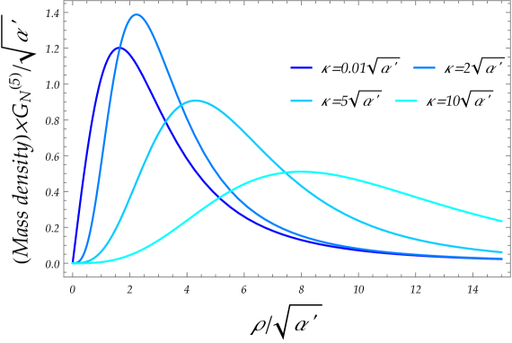
Figure 1: Radial mass density function of the global instanton solution for different values of the instanton scale, $\kappa^{2}$.

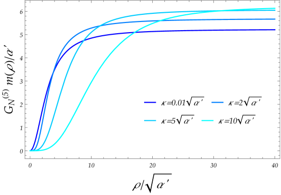
Figure 2: Radial mass function of the global instanton solution for different values of $\kappa^{2}$ obtained by integration of the mass density function in Fig. 1 with respect to $\rho$.

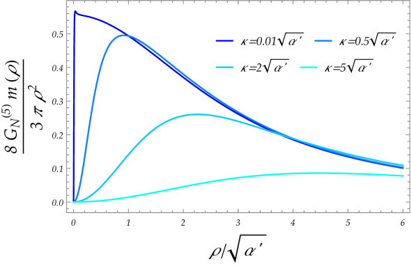
Figure 3: Quotient between the radial mass function of the global instanton solution and the mass of the 5-dimensional Schwarzschild black hole for that Schwarzschild radius for different values of $\kappa^{2}$.

Figure 4: Value of the Kretschmann invariant for the global instanton solution for different values of $\kappa^{2}$.

2 Conclusions

Globally regular solutions supported by elementary fields are quite remarkable. In the case of the 4-dimensional global monopoles [27, 28, 29, 13, 19] we have argued that they represent elementary, non-perturbative states of the theory because they do not modify the entropy of a given Abelian black hole solution when they are added to it. They do contribute to the mass, though. Adding the global instanton to 5-dimensional black holes should have the same result: unmodified entropy and increased mass. However, the reverse seems to happen: the entropy is modified while the mass is not. The construction of the global instanton solution seems to suggest that this is a false appearance caused by an inappropriate definition of the charges involved. The exact role in 4-dimensional non-Abelian black-hole solutions (in which it must appear disguised as a coloured monopole) has to be investigated. It is also unclear if a global instanton can be added to a Schwarzschild-Tangerlini (or any other non-extremal black hole) and what the effect would be.

We have tried to deform this solution by adding angular momentum, which in these theories is always possible, although the simplest ways to do it (adding a non-trivial harmonic function $M$ to generate a non-vanishing $\omega_{5}$) would also introduce a singularity at the origin. While we have succeeded in producing an $\omega_{5}$ regular at $\rho=0$ and dropping at infinity as $\rho^{-2}$, the metric function $\hat{f}^{-1}$ becomes singular at $\rho=0$. It is possible to cancel those singularities by introducing additional Abelian harmonic functions with fine-tuned coefficients but the resulting $\hat{f}^{-1}$ either has zeroes, or leads to negative mass or both.

The non-Abelian solutions found so far in the supergravity/superstring context are the simplest to construct. One can expect, however, a space of solutions far richer than that of the Abelian ones. Work in this direction is under way.

Appendix A The theory

The theory we are considering is a truncation of the effective field theory of the Heterotic Superstring compactified on $T^{5}$ that preserves an SU$(2)$ triplet of vector fields. The compactification and truncation reduce the theory to a particular model of gauged $\mathcal{N}=1,d=5$ supergravity to which one can apply the solution-generating techniques based on the characterization of supersymmetric solutions described in Appendix B. The dimensional reduction of this model on a circle gives the so-called ST$[2,6]$ model of $\mathcal{N}=2,d=4$ supergravity coupled to 6 vector multiplets and we will, therefore, refer to it by that name in the 5-dimensional context as well. Here we are going to give a minimal description of the bosonic sector of these theories and of the particular model we are considering. More information can be found in Refs. [36, 37, 3].

The ST$[2,6]$ model model $\mathcal{N}=1,d=5$ supergravity contains 5 vector supermultiplets labeled by $x,y=1,\cdots,5$, each containing a vector field $A^{x}{}_{\mu}$ and a scalar $\phi^{x}$. Together with the graviphoton $A^{0}{}_{\mu}$, all the vectors are written $A^{I}{}_{\mu}$, $I,J,\ldots=0,1,\cdots,5$. The only remaining bosonic field is the spacetime metric $g_{\mu\nu}$. The $C_{IJK}$ tensor has the non-vanishing components

$$C_{0xy}=\tfrac{1}{6}\eta_{xy}\,,\qquad\mbox{where}\,\,\,\,\,(\eta_{xy})=\mathrm{diag}(+-\dotsm-)\,,$$ (A.1)

and the Real Special manifold parametrized by the physical scalars can be identified with the Riemannian symmetric space

$$\mathrm{SO}(1,1)\times\frac{\mathrm{SO}(1,4)}{\mathrm{SO}(4)}\,.$$ (A.2)

A convenient parametrization of the scalar manifold is

$$h^{0}=e^{-\phi}k^{2/3}\,,\hskip 8.5359pth^{1,2}=k^{-4/3}\left[1\pm(\ell^{2}+\tfrac{1}{2}e^{\phi}k^{2})\right]\,,\hskip 8.5359pth^{3,4,5}=-2k^{-4/3}\ell^{3,4,5}\,,$$ (A.3)

where $\phi$ coincides with the 10-dimensional Heterotic Superstring dilaton field, $k$ is the Kaluza-Klein scalar of the dimensional reduction from $d=6$ to $d=5$ and the $\ell^{A}$ are the fifth components of the 6-dimensional vector fields. The rest of the components that make up the 10-dimensional vector fields have been truncated [39].

The group SO$(3)$ acts in the adjoint on the coordinates $x=3,4,5$ which we are going to denote by $A,B,\ldots$ and this is the sector that is gauged without the use of Fayet-Iliopoulos terms. This means that R-symmetry is not gauged and there is no scalar potential. The structure constants are $f_{AB}{}^{C}=+\varepsilon_{AB}{}^{C}$. We will denote with $a,b,\ldots=1,2$ the ungauged directions. Observe that this sector of the theory corresponds to the so-called STU model: in absence of the $h^{A}$s we can make the linear redefinitions

$$h^{1\prime}\equiv\tfrac{1}{\sqrt{2}}(h^{1}+h^{2})\,,\hskip 28.45274pth^{2\prime}\equiv\tfrac{1}{\sqrt{2}}(h^{1}-h^{2})\,,\,\,\,\,\Rightarrow\,\,\,\,C_{abc}h^{a}h^{b}h^{c}=h^{0}h^{1\prime}h^{2\prime}\,.$$ (A.4)

Thus, our model can be also understood as the STU model with an additional SU$(2)$ triplet of vector multiplets.

With the above parametrization of the scalar manifold, the action for this model can be brought to the form

$$\begin{array}[]{rcl}S&=&{\displaystyle\int d^{5}x\sqrt{g}\ \biggl{\{}R+\partial_{\mu}\phi\partial^{\mu}\phi+\tfrac{4}{3}\partial_{\mu}\log{k}\partial^{\mu}\log{k}+2e^{-\phi}k^{-2}\mathfrak{D}_{\mu}\ell^{A}\mathfrak{D}^{\mu}\ell^{A}}\\ \\ &&-\tfrac{1}{12}e^{2\phi}k^{-4/3}F^{0}\cdot F^{0}+\tfrac{1}{12}\left(\eta_{xy}e^{-\phi}k^{2/3}-9h_{x}h_{y}\right)F^{x}\cdot F^{y}\\ \\ &&+\tfrac{1}{24\sqrt{3}}{\displaystyle\frac{\varepsilon^{\mu\nu\rho\sigma\alpha}}{\sqrt{g}}}A^{0}{}_{\mu}\eta_{xy}F^{x}{}_{\nu\rho}F^{y}{}_{\sigma\alpha}\biggr{\}}\,,\end{array}$$ (A.5)

where

$$\mathfrak{D}_{\mu}\ell^{A} = \partial_{\mu}\ell^{A}+g\varepsilon^{A}{}_{BC}A^{B}{}_{\mu}\ell^{C}\,,$$ (A.6)

$$F^{0,a}{}_{\mu\nu} = 2\partial_{[\mu}A^{0,a}{}_{\nu]}\,,$$ (A.7)

$$F^{A}{}_{\mu\nu} = 2\partial_{[\mu}A^{A}{}_{\nu]}+g\varepsilon^{A}{}_{BC}A^{B}{}_{\mu}A^{C}{}_{\nu}\,.$$ (A.8)

Notice that $A^{0}{}_{\mu}$ is sourced by $\varepsilon^{\mu\nu\rho\sigma\alpha}\eta_{xy}F^{x}{}_{\nu\rho}F^{y}{}_{\sigma\alpha}$ which is related to the instanton number on the constant-time hypersurfaces. In differential-form language, its equation of motion is

$$d(e^{2\phi}k^{-4/3}\star F^{0})=\tfrac{1}{2\sqrt{3}}\eta_{xy}F^{x}\wedge F^{y}=0\,,$$ (A.9)

which is similar to that of the Kalb-Ramond 2-form $B$. This is because $A^{0}$ is the 5-dimensional dual of the dimensionally reduced Heterotic Kalb-Ramond form $B$. The duality relation is

$$F^{0}=e^{-2\phi}k^{4/3}\star H\,,\,\,\,\,\,\mbox{with}\,\,\,\,\,H\equiv dB+\tfrac{1}{2\sqrt{3}}\omega_{\rm CS}\,,$$ (A.10)

where $\omega_{\rm CS}$ is the Chern-Simons 3-form of all the vector fields but $A^{0}$ itself

$$\omega_{\rm CS}=\tfrac{1}{2}F^{+}\wedge A^{-}+\tfrac{1}{2}F^{-}\wedge A+F^{A}\wedge A^{A}-\tfrac{1}{3!}g\epsilon_{ABC}A^{A}\wedge A^{B}\wedge A^{C}\,,$$ (A.11)

satisfying

$$d\omega_{\rm CS}=\eta_{xy}F^{x}\wedge F^{y}\,.$$ (A.12)

Appendix B Timelike supersymmetric solutions

As shown in Refs. [40, 13, 14, 15, 17], the problem of finding timelike supersymmetric solutions of $\mathcal{N}=2,d=4$ SEYM theories and timelike or null supersymmetric solutions with an additional isometry of $\mathcal{N}=1,d=5$ SEYM theories is effectively reduced to a much simpler problem: finding functions $\Phi^{\Lambda},\Phi_{\Lambda}$ and vector fields $\breve{A}^{\Lambda}{}_{\underline{r}}$ in Euclidean 3-dimensional space $\mathbb{E}^{3}$ solving these three sets of equations:

$$\tfrac{1}{2}\varepsilon_{\underline{r}\underline{s}\underline{w}}\breve{F}^{\Lambda}{}_{\underline{s}\underline{w}}-\breve{\mathfrak{D}}_{\underline{r}}\Phi^{\Lambda} = 0\,,$$ (B.1)

$$\breve{\mathfrak{D}}_{\underline{r}}\breve{\mathfrak{D}}_{\underline{r}}\Phi_{\Lambda}-g^{2}f_{\Lambda\Sigma}{}^{\Omega}f_{\Delta\Omega}{}^{\Gamma}\Phi^{\Sigma}\Phi^{\Delta}\Phi_{\Gamma} = 0\,,$$ (B.2)

$$\Phi_{\Lambda}\breve{\mathfrak{D}}_{\underline{r}}\breve{\mathfrak{D}}_{\underline{r}}\Phi^{\Lambda}-\Phi^{\Lambda}\breve{\mathfrak{D}}_{\underline{r}}\breve{\mathfrak{D}}_{\underline{r}}\Phi_{\Lambda} = 0\,,$$ (B.3)

where $\breve{\mathfrak{D}}_{\underline{r}}$ is the gauge covariant derivative in $\mathbb{E}^{3}$ with respect to the connection $\breve{A}^{\Lambda}{}_{\underline{r}}$.

Eqs. (B.1) are the Bogomol’nyi equations [41] for a set of real, adjoint, Higgs fields $\Phi^{\Lambda}$ and gauge vector fields $\breve{A}^{\Lambda}{}_{\underline{r}}$ on $\mathbb{E}^{3}$. In the Abelian case, the integrability conditions are the Laplace equations $\partial_{\underline{r}}\partial_{\underline{r}}\Phi^{\Lambda}=0$ and the vector fields are implicitly determined by the harmonic functions $\Phi^{\Lambda}$. In the non-Abelian sector this is no longer true, and the non-linear equation has to be solved simultaneously for the scalar and the vector fields.

Eqs. (B.2) are equations for the scalar fields $\Phi_{\Lambda}$ linear in them. In the Abelian directions the $\Phi_{\Lambda}$ are harmonic functions $\partial_{\underline{r}}\partial_{\underline{r}}\Phi_{\Lambda}=0$. In the SU$(2)$ directions we are going to set them to zero.

Eq. (B.3) is the integrability condition of the equations that define the 1-forms $\omega_{\underline{r}}$ that appear in the 4- and 5-dimensional metrics

$$\partial_{[\underline{r}}\omega_{\underline{s}]}=2\varepsilon_{rsw}\left(\Phi_{\Lambda}\breve{\mathfrak{D}}_{\underline{w}}\Phi^{\Lambda}-\Phi^{\Lambda}\breve{\mathfrak{D}}_{\underline{w}}\Phi_{\Lambda}\right)\,.$$ (B.4)

and it is guaranteed to be satisfied everywhere except at the loci of the singularities of the scalar functions $\Phi^{\Lambda},\Phi_{\Lambda}$ where it lead to the so-called bubble equations.

For each solution $\Phi^{\Lambda},\Phi_{\Lambda},\breve{A}^{\Lambda}{}_{\underline{r}}$ we can construct two different solutions of the three kinds mentioned above. Here we only need the prescription to construct timelike solutions with an additional isometry of $\mathcal{N}=1,d=5$ SEYM theories:

1. The elementary building blocks, namely the $2(n_{V5}+2)$ functions $M,H,K^{I},L_{I}$ and the 1-forms $\omega,\breve{A}^{I},\chi$ in $\mathbb{E}^{3}$ are related to the functions $\Phi^{\Lambda},\Phi_{\Lambda}$ and 1-forms $\omega,\breve{A}^{\Lambda}{}_{\underline{r}}$ determined by solving Eqs. (B.1)-(B.4) by

   $$\begin{array}[]{rcl}K^{I}&=&\delta^{I}{}_{\Lambda}\Phi^{\Lambda+1}\,,\hskip 19.91684ptL_{I}=-\frac{2\sqrt{2}}{3}\delta_{I}{}^{\Lambda}\Phi_{\Lambda+1}\,,\hskip 19.91684ptH=-2\sqrt{2}\Phi^{0}\,,\hskip 19.91684ptM=+\sqrt{2}\Phi_{0}\,,\\ &&\\ \omega&=&\omega\,,\hskip 19.91684pt\chi_{\underline{r}}=-2\sqrt{2}\breve{A}^{0}{}_{\underline{r}}\,,\hskip 19.91684pt\breve{A}^{I}{}_{\underline{r}}=\delta^{I}{}_{\Lambda}\breve{A}^{\Lambda+1}{}_{\underline{r}}\,,\,\,\,\,\,I=0,\cdots,n_{V5}\,.\end{array}$$ (B.5)

   All the timelike solutions have necessarily $H\neq 0$, ($\Phi^{0}\neq 0$).

2. The Yang-Mills coupling constant that appears in Eqs. (B.1)-(B.3) can be understood as the 4($=1+3$)-dimensional one $g_{4}$. It needs to be replaced by the coupling constant used in the 5-dimensional theory, which is related to it by

   $$g_{4}=-\sqrt{24}g\,.$$ (B.6)

3. With the above building blocks we construct first the combinations

   $$h_{I}/\hat{f} = L_{I}+8C_{IJK}K^{J}K^{K}/H\,,$$ (B.7)

   $$\hat{\omega} = \omega_{5}(dz+\chi)+\omega\,,$$ (B.8)

   $$\omega_{5} = M+16\sqrt{2}H^{-2}C_{IJK}K^{I}K^{J}K^{K}+3\sqrt{2}H^{-1}L_{I}K^{I}\,,$$ (B.9)

   $$\hat{A}^{I} = 2\sqrt{6}\left[H^{-1}K^{I}(dz+\chi)-\breve{A}^{I}\right]\,,$$ (B.10)

   $$\hat{F}^{I} = 2\sqrt{6}\left\{\breve{\mathfrak{D}}\left[K^{I}H^{-1}\wedge(dz+\chi)\right]-\star_{3}H\breve{\mathfrak{D}}K^{I}\right\}\,.$$ (B.11)

4. The physical fields are recovered from the building blocks as follows:

   1. For Real Special manifolds which are Riemannian symmetric manifolds we can use this expression

      $$\begin{array}[]{rcl}\hat{f}^{-3}&=&3^{3}C^{IJK}L_{I}L_{J}L_{K}+3^{4}\cdot 2^{3}C^{IJK}C_{KLM}L_{I}L_{J}K^{L}K^{M}/H\\ &&\\ &&+3\cdot 2^{6}L_{I}K^{I}C_{JKL}K^{J}K^{K}K^{L}/H^{2}+2^{9}\left(C_{IJK}K^{I}K^{J}K^{K}\right)^{2}/H^{3}\,,\end{array}$$ (B.12)

      which for the model at hands reduces to

      $$\begin{array}[]{rcl}\hat{f}^{\,-1}&=&H^{-1}\left\{\tfrac{1}{4}\left(6HL_{0}+8\eta_{xy}K^{x}K^{y}\right)\left[9H^{2}\eta^{xy}L_{x}L_{y}+48HK^{0}L_{x}K^{x}\right.\right.\\ &&\\ &&\left.\left.+64(K^{0})^{2}\eta_{xy}K^{x}K^{y}\right]\right\}^{1/3}\,.\end{array}$$ (B.13)

   2. Using the metric factor we can find the $h_{I}$ from Eq. (B.7) and, from these, the $h^{I}$ using

      $$h^{I}=27C^{IJK}h_{J}h_{K}\,.$$ (B.14)

      The scalar fields $\phi^{x}$ can be obtained by inverting the functions $h_{I}(\phi)$ or $h^{I}(\phi)$. A possible, but not unique, parametrization can be given by

      $$\phi^{x}=h^{x}=9\eta^{xy}h_{y}h_{0}\,.$$ (B.15)

   3. With the previous results the spacetime metric is completely determined and has the form

      $$ds^{2}=\hat{f}^{\,2}(dt+\hat{\omega})^{2}-\hat{f}^{\,-1}\left[H^{-1}(dz+\chi)^{2}+Hdx^{r}dx^{r}\right]\,.$$ (B.16)

   4. The 5-dimensional vector fields are given by

      $$A^{I}=-\sqrt{3}h^{I}e^{0}+\hat{A}^{I}\,,\,\,\,\,\,\mbox{where}\,\,\,\,\,e^{0}\equiv\hat{f}(dt+\hat{\omega})\,,$$ (B.17)

      so that the spatial components, labeled by $m,n=z,1,2,3$, are

      $$A^{I}{}_{\underline{m}}=\hat{A}^{I}{}_{\underline{m}}-\sqrt{3}h^{I}\hat{f}\hat{\omega}_{\underline{m}}\,.$$ (B.18)

References

- [1] M. J. Duff, R. R. Khuri and J. X. Lu, “String solitons,” Phys. Rept. 259 (1995) 213. DOI:10.1016/0370-1573(95)00002-X [hep-th/9412184].
- [2] K. S. Stelle, “BPS branes in supergravity,” In “Trieste 1997, High energy physics and cosmology” 29-127 [hep-th/9803116].
- [3] T. Ortín, “Gravity and Strings”, 2nd edition Cambridge University Press (2015)
-
[4]
I. Bena and N. P. Warner,
“Black holes, black rings and their microstates,”
Lect. Notes Phys. 755 (2008) 1.
DOI:
10.1007/978-3-540-79523-0_1. [hep-th/0701216]. - [5] I. Bena and N. P. Warner, arXiv:1311.4538 [hep-th].
- [6] S. D. Mathur, “The Fuzzball proposal for black holes: An Elementary review,” Fortsch. Phys. 53 (2005) 793 DOI:10.1002/prop.200410203. [hep-th/0502050].
- [7] I. Bena, M. Shigemori and N. P. Warner, “Black-Hole Entropy from Supergravity Superstrata States,” JHEP 1410 (2014) 140. DOI:10.1007/JHEP10(2014)140. [arXiv:1406.4506 [hep-th]].
- [8] I. Bena, S. Giusto, E. J. Martinec, R. Russo, M. Shigemori, D. Turton and N. P. Warner, “Smooth horizonless geometries deep inside the black-hole regime,” Phys. Rev. Lett. 117 (2016) no.20, 201601 DOI:10.1103/PhysRevLett.117.201601 [arXiv:1607.03908 [hep-th]].
- [9] M. S. Volkov and D. V. Gal’tsov, “Gravitating nonAbelian solitons and black holes with Yang-Mills fields,” Phys. Rept. 319 (1999) 1. DOI:10.1016/S0370-1573(99)00010-1. [hep-th/9810070].
- [10] D. V. Gal’tsov, “Gravitating lumps,” Proceedings of the 16th International Conference on General Relativity and Gravitation (GR16), Nigel T. Bishop and Sunil D. Maharaj Eds., World Scientific, Singapore, 2002. hep-th/0112038.
- [11] E. Winstanley, “Classical Yang-Mills black hole hair in anti-de Sitter space,” Lect. Notes Phys. 769 (2009) 49. [arXiv:0801.0527 [gr-qc]].
- [12] M. S. Volkov, “Hairy black holes in the XX-th and XXI-st centuries,” arXiv:1601.08230 [gr-qc].
- [13] M. Hübscher, P. Meessen, T. Ortín and S. Vaulà, “N=2 Einstein-Yang-Mills’s BPS solutions,” JHEP 0809 (2008) 099. DOI:10.1088/1126-6708/2008/09/099. [arXiv:0806.1477 [hep-th]].
- [14] J. Bellorín and T. Ortín, “Characterization of all the supersymmetric solutions of gauged N=1, d=5 supergravity,” JHEP 0708 (2007) 096. DOI:10.1088/1126-6708/2007/08/096. [arXiv:0705.2567 [hep-th]].
- [15] J. Bellorín, “Supersymmetric solutions of gauged five-dimensional supergravity with general matter couplings,” Class. Quant. Grav. 26 (2009) 195012. DOI:10.1088/0264-9381/26/19/195012. [arXiv:0810.0527 [hep-th]].
- [16] P. Bueno, P. Meessen, T. Ortín and P. F. Ramírez, “Resolution of SU(2) monopole singularities by oxidation,” Phys. Lett. B 746 (2015) 109. DOI:10.1016/j.physletb.2015.04.065. [arXiv:1503.01044 [hep-th]].
- [17] P. Meessen, T. Ortín and P. Fernández-Ramírez, “Non-Abelian, supersymmetric black holes and strings in 5 dimensions,” JHEP 1603 (2016) 112. DOI:10.1007/JHEP03(2016)112. [arXiv:1512.07131 [hep-th]].
- [18] P. Meessen, “Supersymmetric coloured/hairy black holes,” Phys. Lett. B 665 (2008) 388. DOI:10.1016/j.physletb.2008.06.035. [arXiv:0803.0684 [hep-th]].
- [19] P. Bueno, P. Meessen, T. Ortin and P. F. Ramirez, “ Einstein-Yang-Mills’ static two-center solutions,” JHEP 1412 (2014) 093. DOI:10.1007/JHEP12(2014)093 [arXiv:1410.4160 [hep-th]].
- [20] P. Meessen and T. Ortín, “ super-EYM coloured black holes from defective Lax matrices,” JHEP 1504 (2015) 100. DOI:10.1007/JHEP04(2015)100. [arXiv:1501.02078 [hep-th]].
- [21] T. Ortín and P. F. Ramírez, “A non-Abelian Black Ring,” Phys. Lett. B 760 (2016) 475. DOI:10.1016/j.physletb.2016.07.018 [arXiv:1605.00005 [hep-th]].
- [22] P. F. Ramírez, “Non-Abelian bubbles in microstate geometries,” JHEP 1611 (2016) 152. DOI:10.1007/JHEP11(2016)152 [arXiv:1608.01330 [hep-th]].
- [23] A. Strominger and C. Vafa, “Microscopic origin of the Bekenstein-Hawking entropy,” Phys. Lett. B 379 (1996) 99. DOI:10.1016/0370-2693(96)00345-0 [hep-th/9601029].
- [24] J. M. Maldacena, “Black holes in string theory,”, Ph.D. Thesis, Princeton University, 1996. hep-th/9607235.
- [25] P. A. Cano, P. Meessen, T. Ortín and P. F. Ramírez, “Non-Abelian black holes in string theory,” arXiv:1704.01134 [hep-th].
- [26] A. A. Belavin, A. M. Polyakov, A. S. Schwartz and Y. S. Tyupkin, “Pseudoparticle Solutions of the Yang-Mills Equations,” Phys. Lett. B 59 (1975) 85. DOI:10.1016/0370-2693(75)90163-X.
- [27] J. A. Harvey and J. Liu, “Magnetic monopoles in N=4 supersymmetric low-energy superstring theory,” Phys. Lett. B 268 (1991) 40. DOI:10.1016/0370-2693(91)90919-H
- [28] A. H. Chamseddine and M. S. Volkov, “NonAbelian BPS monopoles in N=4 gauged supergravity,” Phys. Rev. Lett. 79 (1997) 3343. DOI:10.1103/PhysRevLett.79.3343 [hep-th/9707176].
- [29] A. H. Chamseddine and M. S. Volkov, “NonAbelian solitons in N=4 gauged supergravity and leading order string theory,” Phys. Rev. D 57 (1998) 6242. DOI:10.1103/PhysRevD.57.6242 [hep-th/9711181].
- [30] A. Strominger, “Heterotic solitons,” Nucl. Phys. B 343 (1990) 167. Erratum: [Nucl. Phys. B 353 (1991) 565]. DOI:10.1016/0550-3213(91)90349-3, DOI:10.1016/0550-3213(90)90599-9
- [31] A. P. Protogenov, “Exact Classical Solutions of Yang-Mills Sourceless Equations,” Phys. Lett. B 67 (1977) 62. DOI:10.1016/0370-2693(77)90806-1.
- [32] P.B. Kronheimer, “Monopoles and Taub-NUT spaces,” M.Sc. Dissertation, Oxford University, 1995.
- [33] M. J. Duff, R. R. Khuri and J. X. Lu, “String and five-brane solitons: Singular or nonsingular?,” Nucl. Phys. B 377 (1992) 281. DOI:10.1016/0550-3213(92)90025-7. [hep-th/9112023].
- [34] C. G. Callan, Jr., J. A. Harvey and A. Strominger, “Worldbrane actions for string solitons,” Nucl. Phys. B 367 (1991) 60. DOI:10.1016/0550-3213(91)90041-U.
- [35] C. G. Callan, Jr., J. A. Harvey and A. Strominger, “World sheet approach to heterotic instantons and solitons,” Nucl. Phys. B 359 (1991) 611. DOI:10.1016/0550-3213(91)90074-8
- [36] E. Bergshoeff, S. Cucu, T. de Wit, J. Gheerardyn, S. Vandoren and A. Van Proeyen, “N = 2 supergravity in five-dimensions revisited,” Class. Quant. Grav. 21 (2004) 3015. [Class. Quant. Grav. 23 (2006) 7149]. DOI:10.1088/0264-9381/23/23/C01, DOI:10.1088/0264-9381/21/12/013. [hep-th/0403045].
- [37] D. Z. Freedman and A. Van Proeyen, “Supergravity,” Cambridge University Press, 2012.
- [38] J. Bellorín, P. Meessen and T. Ortín, “All the supersymmetric solutions of N=1,d=5 ungauged supergravity,” JHEP 0701, 020 (2007). DOI:10.1088/1126-6708/2007/01/020. [hep-th/0610196].
- [39] P. A. Cano, T. Ortín and C. Santoli, “Non-Abelian black string solutions of supergravity,” JHEP 1612 (2016) 112. DOI:10.1007/JHEP12(2016)112 [arXiv:1607.02595 [hep-th]].
- [40] M. Hübscher, P. Meessen, T. Ortín and S. Vaulà, “Supersymmetric N=2 Einstein-Yang-Mills monopoles and covariant attractors,” Phys. Rev. D 78 (2008) 065031. DOI:10.1103/PhysRevD.78.065031. [arXiv:0712.1530 [hep-th]].
- [41] E. B. Bogomol’nyi, “Stability of Classical Solutions,” Sov. J. Nucl. Phys. 24 (1976) 449 [Yad. Fiz. 24 (1976) 861].
- [42] G. Etesi and T. Hausel, “New Yang-Mills instantons on multicentered gravitational instantons,” Commun. Math. Phys. 235 (2003) 275. DOI:10.1007/s00220-003-0806-8. [hep-th/0207196].
- [43] P. Meessen, T. Ortín and P.F. Ramírez, in preparation.
- [44] F. Denef, “Supergravity flows and D-brane stability,” JHEP 0008 (2000) 050. DOI:10.1088/1126-6708/2000/08/050. [hep-th/0005049].
- [45] B. Bates and F. Denef, “Exact solutions for supersymmetric stationary black hole composites,” JHEP 1111 (2011) 127. DOI:10.1007/JHEP11(2011)127. [hep-th/0304094].