Spectral Methods for Nonparametric Models

Abstract

Nonparametric models are versatile, albeit computationally expensive, tool for modeling mixture models. In this paper, we introduce spectral methods for the two most popular nonparametric models: the Indian Buffet Process (IBP) and the Hierarchical Dirichlet Process (HDP). We show that using spectral methods for the inference of nonparametric models are computationally and statistically efficient. In particular, we derive the lower-order moments of the IBP and the HDP, propose spectral algorithms for both models, and provide reconstruction guarantees for the algorithms. For the HDP, we further show that applying hierarchical models on dataset with hierarchical structure, which can be solved with the generalized spectral HDP, produces better solutions to that of flat models regarding likelihood performance.

Keywords: Spectral Methods, Indian Buffet Process, Hierarchical Dirichlet Process

1 Introduction

Latent variable models have become ubiquitous in statistical data analysis, spanning over a diverse set of applications ranging from text (Blei et al., 2002), images (Quattoni et al., 2004) to user behavior (Aly et al., 2012). In these works, latent variables are introduced to represent unobserved properties or hidden causes of the observed data. In particular, Bayesian Nonparametrics such as the Dirichlet mixture models (Neal, 1998), the Indian Buffet Process (IBP) (Griffiths and Ghahramani, 2011) and the Hierarchical Dirichlet Process (HDP) (Teh et al., 2006) allow for flexible representation and adaptation in terms model complexity.

In recent years spectral methods have become a credible alternative to sampling (Griffiths and Steyvers, 2004) and variational methods (Blei and Jordan, 2005; Dempster et al., 1977) for the inference of such structures. In particular, the work of Anandkumar et al. (2012b, 2011); Boots et al. (2013); Hsu et al. (2009); Song et al. (2010) demonstrates that it is possible to infer latent variable structure accurately, despite the problem being nonconvex, thus exhibiting many local minima. A particularly attractive aspect of spectral methods is that they allow for efficient means of inferring the model complexity in the same way as the remaining parameters, simply by thresholding eigenvalue decomposition appropriately. This makes them suitable for nonparametric Bayesian approaches.

While the issue of spectral inference with the Dirichlet Distribution is largely settled (Anandkumar et al., 2012b, 2014), the domain of nonparametric tools is much richer and it is therefore desirable to see whether the methods can be extended to popular nonparametric models such as the IBP. As sampling-based methods are computationally expensive for models with complicated hierarchical structure, another attractive direction is to apply spectral method to nonparametric hierarchical model such as the HDP. By using countsketch FFT technique for fast tensor decomposition (Wang et al., 2015), spectral method for the Latent Dirichlet Allocation (LDA), which can be viewed as the simplest case in thespectral algorithm for the HDP, already outperform sampling-based algorithms significantly both in terms of perplexity and speed. Since the time complexity of the proposed spectral method for the HDP does not scale with the number of layers, the algorithm enjoys significant improvement in time over HDP samplers. In a nutshell, this work contributes to completing the tool set of spectral methods. This is an important goal to ensure that entire models can be translated wholly into spectral algorithms, rather than just parts.

We provide a full analysis of the tensors arising from the IBP and the HDP. For the IBP, we show how spectral algorithms need to be modified, since a degeneracy in the third order tensor requires fourth order terms, to successfully infer all the hidden variables. For the HDP, we derive the generalized form in obtaining tensors for any arbitrary hierarchical structure. To recover the parameters and latent factors, we use Excess Correlation Analysis (ECA) (Anandkumar et al., 2012a) to whiten the higher order tensors and to reduce their dimensionality. Subsequently we employ the power method to obtain symmetric factorization of the higher-order terms. The methods provided in this work are simple to implement and have high efficiency in recovering the latent factors and related parameters. We demonstrate how this approach can be used in inferring an IBP structure in the models discussed in Griffiths and Ghahramani (2011) and Knowles and Ghahramani (2007) and the generalized spectral method for the HDP, which can be used in modeling problems involving grouped data such that mixture components are shared across all the groups. Moreover, we show that empirically the spectral algorithms outperform sampling-based algorithms and variational approaches both in terms of perplexity and speed. Statistical guarantees for recovery and stability of the estimates conclude the paper.

Outline: The key idea of spectral methods is to use the method of moments to solve the underlying parameters, which includes the following steps:

• Construct equations for obtaining diagonalized tensors using moments of the latent variables defined in the probabilistic graphical model.

• Replace the theoretical moments with the empirical moments and obtain an empirical version of the diagonalized tensor.

• Use tensor decomposition solvers to decompose the empirical diagonalized tensor and obtain its eigenvalues/eigenvectors, which corresponds to the desired hidden vectors/topics.

In order to use tensor decomposition solver, a decomposable symmetric tensor must be constructed. A tensor is decomposable and symmetric if it can be written as a summation of the outer products of its eigenvectors weighted by their correspnding eigenvalues. In the two dimensional case (i.e, as a matrix), a rank-k symmetric tensor is decomposable and symmetric since it can be decomposed as $M=\sum_{i=1}^{k}\lambda_{i}v_{i}v_{i}^{T},$ where $\lambda_{i}/v_{i}$ are the eigenvalue/eigenvector pairs. In the first step, we construct a tensor that has such properties using theoretical moments so that the tensor can be further estimated using empirical moments and decomposed by tensor decomposition tools.

The paper is structured as follows: In Section 2 we introduce the IBP and the HDP models. In Section 3 we construct equations for obtaining the diagonalized tensors using moments of the IBP and apply them on two applications, the linear Gaussian latent factor model and the infinte sparse factor analysis. We also derive the generalized tensors for the HDP that are applicable on any arbitrary hierarchical structure. In Section 4 the spectral algorithms for thel IBP and the HDP is proposed. We also list out several tensor decomposition tools that can be used to solve our problem. In Section 5 we show the concentration measure of moments and tensors for these two models and provide overall guarantees on $L_{2}$ distance between the recovered latent vectors and the ground truth. In Section 6 we demonstrate the power of the spectral IBP by showing that the method is able to produce comparable results to that of variational approaches with much lesser time. We also applied it on image data and gene expression data to show that the algorithm is able to infer mearningful patterns in real data. For the spectral method for the HDP, we show that (1) computational does not increase with number of layer using our method, while obviously the factor will significantly affect Gibbs sampling and (2) when the number of samples underneath each nodes in a hierarchical structure is highly unbalanced, the spectral for the HDP is able to obtain solutions better than that of spectral LDA in terms of perplexity.

2 Model Settings

We begin with defining the models of the IBP and the HDP.

2.1 The Indian Buffet Process

The Indian Buffet Process defines a distribution over equivalence classes of binary matrices $Z$ with a finite number of rows and a (potentially) infinite number of columns (Griffiths and Ghahramani, 2006, 2011). The idea is that this allows for automatic adjustment of the number of binary entries, corresponding to the number of independent sources, underlying causes, etc. This is a very useful strategy and it has led to many applications including structuring Markov transition matrices (Fox et al., 2010), learning hidden causes with a bipartite graph (Wood et al., 2006) and finding latent features in link prediction (Miller et al., 2009). Denote by $n\in\mathbb{N}$ the number of rows of $Z$, i.e. the number of customers sampling dishes from the “ Indian Buffet”, let $m_{k}$ be the number of customers who have sampled dish $k$, let $K_{+}$ be the total number of dishes sampled, and denote by $K_{h}$ the number of dishes with a particular selection history $h\in\left\{0;1\right\}^{n}$. That is, $K_{h}>1$ only if there are two or more dishes that have been selected by exactly the same set of customers. Then the probability of generating a particular matrix $Z$ is given by Griffiths and Ghahramani (2011)

$$p(Z)=\frac{\alpha^{K_{+}}}{\prod_{h}K_{h}!}\exp\Biggl{[}{-\alpha\sum_{j=1}^{n}\textstyle\frac{1}{j}}\Biggr{]}\prod_{k=1}^{K_{+}}\frac{(n-m_{k})!(m_{k}-1)!}{n!}$$ (1)

Here $\alpha$ is a parameter determining the expected number of nonzero columns in $Z$. Due to the conjugacy of the prior an alternative way of viewing $p(Z)$ is that each column (aka dish) contains nonzero entries $Z_{ij}$ that are drawn from the binomial distribution $Z_{ij}\sim\mathrm{Bin}(\pi_{i})$. That is, if we knew $K_{+}$, i.e. if we knew how many nonzero features $Z$ contains, and if we knew the probabilities $\pi_{i}$, we could draw $Z$ efficiently from it. We take this approach in our analysis: determine $K_{+}$ and infer the probabilities $\pi_{i}$ directly from the data. This is more reminiscent of the model used to derive the IBP — a hierarchical Beta-Binomial model, albeit with a variable number of entries:

In general, the binary attributes $Z_{ij}$ are not observed. Instead, they capture auxiliary structure pertinent to a statistical model of interest. To make matters more concrete, consider the following two models proposed by Griffiths and Ghahramani (2011) and Knowles and Ghahramani (2007). They also serve to showcase the algorithm design in our paper.

Linear Gaussian Latent Feature Model (Griffiths and Ghahramani, 2011).

The assumption is that we observe vectorial data $x$. It is generated by linear combination of dictionary atoms $\Phi$ and an associated unknown number of binary causes $z$, all corrupted by some additive noise $\epsilon$. That is, we assume that

$$x=\Phi z+\epsilon\text{ where }\epsilon\sim\mathcal{N}(0,\sigma^{2}\mathbf{1})\text{ and }z\sim\mathrm{IBP}(\alpha).$$ (2)

The dictionary matrix $\Phi$ is considered to be fixed but unknown. In this model our goal is to infer both $\Phi$, $\sigma^{2}$ and the probabilities $\pi_{i}$ associated with the IBP model. Given that, a maximum-likelihood estimate of $Z$ can be obtained efficiently.

Infinite Sparse Factor Analysis (Knowles and Ghahramani, 2007).

A second model is that of sparse independent component analysis. In a way, it extends (2) by replacing binary attributes with sparse attributes. That is, instead of $z$ we use the entry-wise product $z\mathrm{.*}y$. This leads to the model

$$x=\Phi(z\mathrm{.*}y)+\epsilon\text{ where }\epsilon\sim\mathcal{N}(0,\sigma^{2}\mathbf{1})\text{ , }z\sim\mathrm{IBP}(\alpha)\text{ and }y_{i}\sim p(y)$$ (3)

Again, the goal is to infer the dictionary $\Phi$, the probabilities $\pi_{i}$ and then to associate likely values of $Z_{ij}$ and $Y_{ij}$ with the data. In particular, Knowles and Ghahramani (2007) make a number of alternative assumptions on $p(y)$, namely either that it is iid Gaussian or that it is iid Laplacian. Note that the scale of $y$ itself is not so important since an equivalent model can always be found by re-scaling matrix $\Phi$ suitably.

Note that in (3) we used the shorthand $\mathrm{.*}$ to denote point-wise multiplication of two vectors in ’Matlab’ notation. While (2) and (3) appear rather similar, the latter model is considerably more complex since it not only amounts to a sparse signal but also to an additional multiplicative scale. Knowles and Ghahramani (2007) refer to the model as Infinite Sparse Factor Analysis (isFA) or Infinite Independent Component Analysis (iICA) depending on the choice of $p(y)$ respectively.

2.2 The Hierarchical Dirichlet Process (HDP)

The HDP mixture models are useful in modeling problems involving groups of data, where each observation within a group is drawn from a mixture model and it is desirable to share mixture components across all the groups. A natural application with this property is topic modeling for documents, possibly supplemented by an ontology. The HDP (Teh et al., 2006) uses a Dirichlet Process (DP) (Antoniak, 1974; Ferguson, 1973) $G_{j}$ for each group $j$ of data to handle uncertainty in number of mixture components. At the same time, in order to share mixture components and clusters across groups, each of these DPs is drawn from a global DP $G_{0}$. The associated graphical model is given below:

More formally, we have the following statistical description of a two level HDP. Extensions to more than two levels are straightforward (we provide a general multilevel HDP spectral inference algorithm).

1. Sample $G_{0}|\gamma_{0},H\sim\mathrm{DP}(\gamma,H)$

2. For each $i\in\left\{I\right\}$ do

   1. Sample $G_{i}|\gamma_{1},G_{0}\sim\mathrm{DP}(\gamma_{0},G_{0})$

   2. For each $j\in\left\{N_{i}\right\}$ do

      1. Sample $\theta_{ij}\sim G_{i}$

      2. Sample $x_{ij}|\theta_{ij}\sim F(\theta_{ij}),$

Here $H$ is the base distribution which governs the a priori distribution over data items, $\gamma_{0}$ is a concentration parameter which controls the amount of sharing across groups and $\gamma_{1}$ is a concentration parameter which governs the a priori number of clusters and a parametric distribution $F(\theta)$. This process can be repeated to achieve deeper hierarchies, as needed.

More formally, we have the following statistical description of a $L$-level HDP.

Figure 1: Hierarchical Dirichlet Process with observations at the leaf nodes.

Trees

Denote by $\mathcal{T}=(V,E)$ a tree of depth $L$. For any vertex ${\bf i}\in\mathcal{T}$ we use $p({\bf i})\in V$, $c({\bf i})\subset V$ and $l({\bf i})\in\left\{0,1...,L-1\right\}$ to denote the parent, the set of children and level of the vertex respectively. When needed, we enumerate the vertices of $\mathcal{T}$ in dictionary order. For instance, the root node is denoted by ${\bf i}=(0)$, whereas ${\bf i}=(0,4,2)$ is the node obtained by picking the fourth child of the root node and then the second child thereof respectively. Finally, we have sets of observations $X_{{\bf i}}$ associated with the vertices ${\bf i}$ (in some cases only the leaf nodes may contain observations). This yields

$$G_{0} \sim\mathrm{DP}(H,\gamma_{0}) \theta_{{\bf i}j} \sim G_{{\bf i}}$$

$$G_{{\bf i}} \sim\mathrm{DP}\left(G_{p({\bf i})},\gamma_{l({\bf i})}\right) x_{{\bf i}j} \sim\mathrm{Categorical}(\theta_{{\bf i}j})$$

Here $\gamma_{{\bf i}}$ denotes the concentration parameter at vertex ${\bf i}$ and $H$ is the base distribution which governs the a priori distribution over data items. Figure 1 illustrates the full model.

As explained earlier, the distributions $G_{\bf i}$ have a stick breaking representation sharing common atoms:

$$G_{\bf i}=\sum_{v=1}^{\infty}\pi_{{\bf i}v}\delta_{\phi_{v}}\text{ with }\phi_{v}\sim H.$$ (4)

3 Spectral Characterization

We are now in a position to define the moments of the IBP and the HBP. Our analysis begins by deriving moments for the IBP proper. Subsequently we apply this to the two models described above. Next, following the similar procedure, we derive the moments for the HDP. All proofs are deferred to the Appendix. For notational convenience we denote by $\mathfrak{S}$ the symmetrized version of a tensor where care is taken to ensure that existing multiplicities are satisfied. That is, for a generic third order tensor we set $\mathfrak{S}_{6}[A]_{ijk}=A_{ijk}+A_{kij}+A_{jki}+A_{jik}+A_{kji}+A_{ikj}$. However, if e.g. $A=B\otimes C$ with $B_{ij}=B_{ji}$, we only need $\mathfrak{S}_{3}[A]_{ijk}=A_{ijk}+A_{jki}+A_{kij}$ to obtain a symmetric tensor.

3.1 Tensorial Moments for the IBP

In our approach we assume that $Z\sim\mathrm{IBP}(\alpha)$. We assume that the number of nonzero attributes $k$ is unknown (but fixed). In our derivation, a degeneracy in the third order tensor requires that we compute a fourth order moment. We can exclude the cases of $\pi_{i}=0$ and $\pi_{i}=1$ since the former amounts to a nonexistent feature and the latter to a constant offset. We use $M_{i}$ to denote moments of order $i$ and $S_{i}$ to denote diagonal(izable) tensors of order $i$. Finally, we use $\pi\in\mathbb{R}^{K_{+}}$ to denote the vector of probabilities $\pi_{i}$.

Order 1

This is straightforward, since we have

$$M_{1}:=\mathbf{E}_{z}\left[z\right]=\pi=:S_{1}.$$ (5)

Order 2

The second order tensor is given by

$$M_{2} :=\mathbf{E}_{z}\left[z\otimes z\right]=\pi\otimes\pi+\mathrm{diag}\left(\pi-\pi^{2}\right)={S}_{1}\otimes{S}_{1}+\mathrm{diag}\left(\pi-\pi^{2}\right).$$ (6)

Solving for the diagonal tensor we have

$$S_{2} :={M}_{2}-{S}_{1}\otimes{S}_{1}=\mathrm{diag}\left(\pi-\pi^{2}\right).$$ (7)

The degeneracies $\left\{0,1\right\}$ of $\pi-\pi^{2}=(1-\pi)\pi$ can be ignored since they amount to non-existent and degenerate probability distributions.

Order 3

The third order moments yield

$${M}_{3}:= \mathbf{E}_{z}\left[z\otimes z\otimes z\right]=\pi\otimes\pi\otimes\pi+\mathfrak{S}_{3}\left[\pi\otimes\mathrm{diag}\left(\pi-\pi^{2}\right)\right]+\mathrm{diag}\left(\pi-3\pi^{2}+2\pi^{3}\right)$$ (8)

$$= {S}_{1}\otimes{S}_{1}\otimes{S}_{1}+\mathfrak{S}_{3}\left[{S}_{1}\otimes{S}_{2}\right]+\mathrm{diag}\left(\pi-3\pi^{2}+2\pi^{3}\right).$$ (9)

$${S}_{3}:= {M}_{3}-\mathfrak{S}_{3}\left[{S}_{1}\otimes{S}_{2}\right]-{S}_{1}\otimes{S}_{1}\otimes{S}_{1}=\mathrm{diag}\left(\pi-3\pi^{2}+2\pi^{3}\right).$$ (10)

Note that the polynomial $\pi-3\pi^{2}+2\pi^{3}=\pi(2\pi-1)(\pi-1)$ vanishes for $\pi=\frac{1}{2}$. This is undesirable for the power method — we need to compute a fourth order tensor to exclude this.

Order 4

The fourth order moments are

$${M}_{4}:= \mathbf{E}_{z}\left[z\otimes z\otimes z\otimes z\right]={S}_{1}\otimes{S}_{1}\otimes{S}_{1}\otimes{S}_{1}+\mathfrak{S}_{6}\left[{S}_{2}\otimes{S}_{1}\otimes{S}_{1}\right]+\mathfrak{S}_{3}\left[{S}_{2}\times{S}_{2}\right]$$

$$+\mathfrak{S}_{4}\left[{S}_{3}\otimes{S}_{1}\right]+\mathrm{diag}\left(\pi-7\pi^{2}+12\pi^{3}-6\pi^{4}\right)$$

$${S}_{4}:= {M}_{4}-{S}_{1}\otimes{S}_{1}\otimes{S}_{1}\otimes{S}_{1}-\mathfrak{S}_{6}\left[{S}_{2}\otimes{S}_{1}\otimes{S}_{1}\right]-\mathfrak{S}_{3}\left[{S}_{2}\times{S}_{2}\right]-\mathfrak{S}_{4}\left[{S}_{3}\otimes{S}_{1}\right]$$

$$= \mathrm{diag}\left(\pi-7\pi^{2}+12\pi^{3}-6\pi^{4}\right).$$ (11)

The roots of the polynomial are $\left\{0,\frac{1}{2}-1/\sqrt{12},\frac{1}{2}+1/\sqrt{12},1\right\}$. Hence the latent factors and their corresponding $\pi_{k}$ can be inferred either by ${S}_{3}$ or by ${S}_{4}$.

3.2 Applications of the IBP

The above derivation showed that if we were able to access $z$ directly, we could infer $\pi$ from it by reading off terms from a diagonal tensor. Unfortunately, this is not quite so easy in practice since $z$ generally acts as a latent attribute in a more complex model. In the following we show how the models of (2) and (3) can be converted into spectral form. We need some notation to indicate multiplications of a tensor $M$ of order $k$ by a set of matrices $A_{i}$.

$$\left[T(M,A_{1},\ldots,A_{k})\right]_{i_{1},\ldots i_{k}}:=\sum_{j_{1},\ldots j_{k}}M_{j_{1},\ldots j_{k}}\left[A_{1}\right]_{i_{1}j_{1}}\cdot\ldots\cdot\left[A_{k}\right]_{i_{k}j_{k}}.$$ (12)

Note that this includes matrix multiplication. For instance, $A_{1}^{\top}MA_{2}=T(M,A_{1},A_{2})$. Also note that in the special case where the matrices $A_{i}$ are vectors, this amounts to a reduction to a scalar. Any such reduced dimensions are assumed to be dropped implicitly. The latter will become useful in the context of the tensor power method in Anandkumar et al. (2012b).

Here are two tensor operations that are frequently used in the derivation for linear applications of the IBP. First, for $x=Az$ (e.g. observation $x$ is a linear combination of some columns in matrix $A$ indicated by the IBP binary vector $z$), the $i$-th order moment $M_{i}^{x}$ where the superscript denotes the variable for the moments, can be obtained by multiplying the $i$-th order moment of $z,$ $M_{i}^{z},$ with the affine matrix $A$ on all dimension, i.e.,

$$M_{i}^{z}=T(M_{i}^{z},A,\cdots,A)$$ (13)

Another property is addition. Suppose $y=x+\sigma$ (e.g. there exists some additional noise.), then, by using addition rule of expectation, we have

$$M_{1}^{y}=M_{1}^{x}+M_{1}^{\sigma}$$ (14)

Higher order moments can be obtained by taking the expansion of the polynomial expression $(x+\sigma)^{\otimes k},$ which yields

$$M_{2}^{y}=\mathbf{E}[(x+\sigma)\otimes(x+\sigma)]=M_{2}^{x}+M_{2}^{\sigma}+\mathfrak{S}_{2}\left(\mathbf{E}\left[x\sigma\right]\right)$$ (15)

$$M_{3}^{y}=M_{3}^{x}+M_{3}^{\sigma}+\mathfrak{S}_{3}\left[x\otimes x\otimes\sigma+\sigma\otimes\sigma\otimes x\right]$$ (16)

$$M_{4}^{y}=M_{4}^{x}+M_{4}^{\sigma}+\mathfrak{S}_{4}\left[\sigma\otimes\sigma\otimes\sigma\otimes x+\sigma\otimes x\otimes x\otimes x\right]+\mathfrak{S}_{6}\left[\sigma\otimes\sigma\otimes x\otimes x\right]$$ (17)

If $\sigma$ is Gaussian or some symmetric random variable, then its first and third moments become zero, thus the third order moment becomes $M_{3}^{y}=M_{3}^{x}+\mathfrak{S}_{3}\left[\sigma\otimes\sigma\otimes x\right].$ Similarly, the forth-order moment reduces to $M_{4}^{y}=M_{4}^{x}+M_{4}^{\sigma}+\mathfrak{S}_{6}\left[\sigma\otimes\sigma\otimes x\otimes x\right].$

Linear Gaussian Latent Factor Model. When dealing with (2) our goal is to infer both $\Phi$ and $\pi$. The main difference is that rather than observing $z$ we have $\Phi z$, hence all tensors are colored. Moreover, we also need to deal with the terms arising from the additive noise $\epsilon$. This yields

$$S_{1}:= M_{1}=T(\pi,\Phi)$$ (18)

$$S_{2}:= M_{2}-S_{1}\otimes S_{1}-\sigma^{2}\mathbf{1}=T(\mathrm{diag}(\pi-\pi^{2}),\Phi,\Phi)$$ (19)

$$S_{3}:= M_{3}-S_{1}\otimes S_{1}\otimes S_{1}-\mathfrak{S}_{3}\left[S_{1}\otimes S_{2}\right]-\mathfrak{S}_{3}\left[{m_{1}\otimes\mathbf{1}}\right]=T\left(\mathrm{diag}\left(\pi-3\pi^{2}+2\pi^{3}\right),\Phi,\Phi,\Phi\right)$$ (20)

$$S_{4}:= M_{4}-S_{1}\otimes S_{1}\otimes S_{1}\otimes S_{1}-\mathfrak{S}_{6}\left[S_{2}\otimes S_{1}\otimes S_{1}\right]-\mathfrak{S}_{3}\left[S_{2}\otimes S_{2}\right]-\mathfrak{S}_{4}\left[S_{3}\otimes S_{1}\right]$$ (21)

$$-\sigma^{2}\mathfrak{S}_{6}\left[S_{2}\otimes\mathbf{1}\right]-m_{4}\mathfrak{S}_{3}\left[\mathbf{1}\otimes\mathbf{1}\right]$$

$$= T\left(\mathrm{diag}\left(-6\pi^{4}+12\pi^{3}-7\pi^{2}+\pi\right),\Phi,\Phi,\Phi,\Phi\right)$$

Here we used the auxiliary statistics $m_{1}$ and $m_{4}$. Denote by $v$ the eigenvector with the smallest eigenvalue of the covariance matrix of $x$. Then the auxiliary variables are defined as

$$m_{1}:= \mathbf{E}_{x}\left[x\left\langle v,\left(x-\mathbf{E}\left[x\right]\right)\right\rangle^{2}\right]=\sigma^{2}T(\pi,\Phi)$$ (22)

$$m_{4}:= \mathbf{E}_{x}\left[\left\langle v,\left(x-\mathbf{E}_{x}\left[x\right]\right)\right\rangle^{4}\right]/3=\sigma^{4}.$$ (23)

These terms are used in a tensor power method to infer both $\Phi$ and $\pi.$

Proof.

To easily apply the addition property of moments, we define $y=\Phi x.$

Order 1 tensor:

By using Equation (5), we have

$$S_{1}:=M_{1} =\mathbf{E}_{x}\left[x\right]=M_{1}^{y}+M_{1}^{\sigma}=T(\mathbf{E}[z],\Phi)=T(\pi,\Phi),$$ (24)

where we apply the addition property of moments in the third equation, and linear transformation property at the fourth equation. To infer the number of latent variables $k$ and deal with the noise term, we need to determine the rank of the covariance matrix $\mathbf{E}_{x}\left[\left(x-\mathbf{E}_{x}{\left[x\right]}\right)\otimes\left(x-\mathbf{E}_{x}{\left[x\right]}\right)\right]$. Because there is additive noise, the smallest $(d-K)$ eigenvalues will not be exactly zero. Instead, they amount to the variance arising from $\epsilon$ since

$$\mathrm{cov}[\Phi z+\epsilon]=\Phi^{\top}\mathrm{cov}[z]\Phi+\mathrm{cov}[\epsilon].$$ (25)

Consequently the smallest eigenvalues of the covariance matrix of $x$ allow us to read off the variance $\sigma^{2}$: for any normal vector $v$ corresponding to the $d-k$ smallest eigenvalues we have

$$\mathbf{E}_{x}\left[\left(v^{\top}\left(x-\mathbf{E}\left[X\right]\right)\right)^{2}\right]=v^{\top}\Phi^{\top}\mathrm{cov}[z]\Phi v+v^{\top}\mathrm{cov}[\epsilon]v=\sigma^{2}.$$ (26)

Order 2 tensor:

Here we plug in Equation (7) and use independence of $z$ and $\epsilon$. Linear terms in $\epsilon$ vanish. Thus we get

$$M_{2}= M_{2}^{y}+M_{2}^{\sigma}+\mathbf{E}[y\otimes\sigma]=T\left(\mathbf{E}_{z}\left[z\otimes z\right],\Phi,\Phi\right)+\sigma^{2}\mathbf{1}$$

$$= T\left(\pi\otimes\pi+\mathrm{diag}\left(\pi-\pi^{2}\right),\Phi,\Phi\right)+\sigma^{2}\mathbf{1}$$ (27)

$$= S_{1}\otimes S_{1}+T\left(\mathrm{diag}\left(\pi-\pi^{2}\right),\Phi,\Phi\right)+\sigma^{2}\mathbf{1},$$ (28)

where the second equations follow the linear transformation property of moments. This yields the statement in Equation (19).

Order 3 tensor:

As before, denote by $v$ an eigenvector corresponding to the $(d-k)$ smallest eigenvalues, i.e. $v^{\top}\Phi=0$. We first define an auxiliary term

$$m_{1}:= \mathbf{E}_{x}\left[x\left(v^{\top}\left(x-\mathbf{E}{\left[x\right]}\right)\right)^{2}\right]=\mathbf{E}_{x}\left[x\left(v^{\top}\left(\Phi\left(z-\pi\right)+\varepsilon\right)\right)^{2}\right]$$

$$= \mathbf{E}_{x}\left[x\left(v^{\top}\varepsilon\right)^{2}\right]=\sigma^{2}T(\pi,\Phi).$$ (29)

Since the Normal Distribution is symmetric, only even moments of $\epsilon$ survive. Using (10), the third order moments yield

$$M_{3} =M_{3}^{y}+\mathbf{E}_{z}\left[\mathfrak{S}_{3}\left[\Phi z\otimes\epsilon\otimes\epsilon\right]\right]$$ (30)

$$=T\left(\mathbf{E}_{z}[z\otimes z\otimes z],\Phi,\Phi,\Phi\right)+\mathfrak{S}_{3}\left(m_{1}\otimes\mathbf{1}\right)$$ (31)

$$=S_{1}\otimes S_{1}\otimes S_{1}+\mathfrak{S}_{3}\left[S_{1}\otimes S_{2}\right]+T\left(\mathrm{diag}\left(\pi-3\pi_{i}^{2}+2\pi_{i}^{3}\right),\Phi,\Phi,\Phi\right)+\mathfrak{S}_{3}\left(m_{1}\otimes\mathbf{1}\right)$$

Thus, we get Equation (20).

Order 4 tensor:

We obtain the fourth-order tensor by first calculating an auxiliary variable related to the additive noise term

$$m_{4}:= \mathbf{E}_{x}\left[\left(v^{\top}\left(x-\mathbf{E}_{x}\left[x\right]\right)\right)^{4}\right]/3=\mathbf{E}[\left(v^{\top}\epsilon\right)^{4}]/3=\sigma^{4}.$$ (32)

Here the last equality followed from the isotropy of Gaussians. With Equation (Order 4), the forth order moments are

$$M_{4}= M_{4}^{y}+M_{4}^{\epsilon}+\mathbf{E}_{x}\left[\mathfrak{S}_{6}\left[y\otimes y\otimes\epsilon\otimes\epsilon\right]\right]$$

$$= T\left(\mathbf{E}_{z}\left[z\otimes z\otimes z\otimes z\right],\Phi,\Phi,\Phi,\Phi\right)+\sigma^{2}\mathfrak{S}_{6}\left[S_{2}\otimes\mathbf{1}\right]+\sigma^{4}\mathfrak{S}_{3}\left[\mathbf{1}\otimes\mathbf{1}\right]$$

$$= S_{1}\otimes S_{1}\otimes S_{1}\otimes S_{1}+\mathfrak{S}_{6}\left[S_{2}\otimes S_{1}\otimes S_{1}\right]+\mathfrak{S}_{3}\left[S_{2}\times S_{2}\right]+\mathfrak{S}_{4}\left[S_{3}\otimes S_{1}\right]$$

$$+T\left(\mathrm{diag}\left(-6\pi^{4}+12\pi^{3}-7\pi^{2}+\pi\right),\Phi,\Phi,\Phi\right)+\sigma^{2}\mathfrak{S}_{6}\left[S_{2}\otimes\mathbf{1}\right]+m_{4}\mathfrak{S}_{3}\left[\mathbf{1}\otimes\mathbf{1}\right].$$

∎

Infinite Sparse Factor Analysis (isFA)

Using the model of (3) it follows that $z$ is a symmetric distribution with mean $0$ provided that $p(y)$ has this property. Here we state the property of moments by using such prior. For $x=z\odot y,$ $M_{i}^{x}=M_{i}^{z}\odot M_{i}^{y}.$ If $y$ is symmetric so that the first and the third order moments vanish, we have $M_{1}^{x}=M_{3}^{x}=0.$ From that it follows that the first and third order moments and tensors vanish, i.e. $S_{1}=0$ and $S_{3}=0$. We have the following statistics:

$$S_{2}:= M_{2}-\sigma^{2}\mathbf{1}=T\left(c\cdot\mathrm{diag}(\pi),\Phi,\Phi\right)$$ (33)

$$S_{4}:= M_{4}-\mathfrak{S}_{3}\left[S_{2}\otimes S_{2}\right]-\sigma^{2}\mathfrak{S}_{6}\left[S_{2}\otimes\mathbf{1}\right]-m_{4}\mathfrak{S}_{3}\left[\mathbf{1}\otimes\mathbf{1}\right]=T\left(\mathrm{diag}(f(\pi)),\Phi,\Phi,\Phi,\Phi\right).$$ (34)

Here $m_{4}$ is defined as in (23). Whenever $p(y)$ in (3) is Gaussian, we have $c=1$ and $f(\pi)=\pi-\pi^{2}$. Moreover, whenever $p(y)$ follows the Laplace distribution, we have $c=2$ and $f(\pi)=24\pi-12\pi^{2}$.

Proof.

Since both $Y$ and $\epsilon$ are symmetric and have zero mean, the odd order tensors vanish. That is $M_{1}=0$ and $M_{3}=0$. It suffices for us to focus on the even terms.

Order 2 tensor:

Using covariance matrix of (7) yields

$$M_{2} =\mathbf{E}_{x}\left[x\otimes x\right]=T\left(\mathbf{E}_{z}{\left[\left(z\odot y\right)\otimes\left(z\odot y\right)\right]},\Phi,\Phi\right)+\sigma^{2}\mathbf{1}$$ (35)

$$=T\left(\left(\mathbf{E}_{z}{\left[z\otimes z\right]}\odot\mathbf{E}_{y}\left[y^{2}\right]\mathbf{1}\right),\Phi,\Phi\right)+\sigma^{2}\mathbf{1}$$ (36)

$$=T\left(\left(\pi\otimes\pi+\mathrm{diag}\left(\pi-\pi^{2}\right)\right)\odot\mathbf{E}_{y}\left[y^{2}\right]\mathbf{1},\Phi,\Phi\right)+\sigma^{2}\mathbf{1}$$ (37)

$$=T\left(\mathbf{E}_{y}\left[y^{2}\right]\mathrm{diag}\left(\pi\right),\Phi,\Phi\right)+\sigma^{2}\mathbf{1}=T\left(\mathrm{diag}\left(\pi\right),\Phi,\Phi\right)+\sigma^{2}\mathbf{1},$$ (38)

where the second equation follows the element-wise multiplication property of the moment. As before, the variance $\sigma^{2}$ of $\epsilon$ can be inferred by Equation (26). Here we get Equation (33).

Order 4 tensor:

With Equation (Order 4) and $\mathbf{E}_{y}\left[y^{4}\right]=3$, we have

$$M_{4}= \mathbf{E}_{x}\left[x\otimes x\otimes x\otimes x\right]$$

$$= \mathbf{E}_{z}{\left[\Phi\left(z\odot y\right)\otimes\Phi\left(z\odot y\right)\otimes\Phi\left(z\odot y\right)\otimes\Phi\left(z\odot y\right)\right]}$$

$$+\mathbf{E}_{z}{\left[\mathfrak{S}_{6}\left[\Phi\left(z\odot y\right)\otimes\Phi\left(z\odot y\right)\otimes\epsilon\otimes\epsilon\right]\right]}+\mathbf{E}\left[\epsilon\otimes\epsilon\otimes\epsilon\otimes\epsilon\right]$$

$$= T\left(\mathbf{E}_{z}\left[z\otimes z\otimes z\otimes z\right]\odot\mathbf{E}_{y}\left[y^{4}\right]\mathbf{1},\Phi,\Phi,\Phi,\Phi\right)+\sigma^{2}\mathfrak{S}_{6}\left[S_{2}\otimes\mathbf{1}\right]+\sigma^{4}\mathfrak{S}_{3}\left[\mathbf{1}\otimes\mathbf{1}\right]$$

$$= \mathfrak{S}_{3}\left[S_{2}\otimes S_{2}\right]+T\left(\mathrm{diag}\left(\mathbf{E}_{y}\left[y^{4}\right]\pi_{i}-3\mathbf{E}_{y}\left[y^{2}\right]^{2}\pi_{i}^{2}\right),\Phi,\Phi,\Phi,\Phi\right)$$

$$+\sigma^{2}\mathfrak{S}_{6}\left[S_{2}\otimes\mathbf{1}\right]+\sigma^{4}\mathfrak{S}_{3}\left[\mathbf{1}\otimes\mathbf{1}\right]$$ (39)

$$= \mathfrak{S}_{3}\left[S_{2}\otimes S_{2}\right]+T\left(3\left(\pi_{i}-\pi_{i}^{2}\right),\Phi,\Phi,\Phi,\Phi\right)+\sigma^{2}\mathfrak{S}_{6}\left[S_{2}\otimes\mathbf{1}\right]+m_{4}\mathfrak{S}_{3}\left[\mathbf{1}\otimes\mathbf{1}\right]$$

where $m_{4}$ can be inferred by (23).

If the prior on $Y$ is drawn from a Laplace distribution the model is called an infinite Inde-pendent Component Analysis (iICA) (Knowles and Ghahramani, 2007). The lower-order moments are similar to that of isFA, except for $\mathbf{E}_{y}\left[y^{2}\right]=2$ and $\mathbf{E}_{y}\left[y^{4}\right]=24$. Replacing these terms in Equation (38) and (39) yields the claim. ∎

Lemma 1

Any linear model of the form (2) or (3) with the property that $\epsilon$ is symmetric and satisfies $\mathbf{E}[\epsilon^{i}]=0$ for $i\in\{1,3,5,\cdots\},$ the same properties for $y$, will yield the same moments.

Proof.

This follows directly from the fact that $z$, $\epsilon$ and $y$ are independent and that the latter two have zero mean and are symmetric. Hence the expectations carry through regardless of the actual underlying distribution. ∎

3.3 Tensorial Moments for the HDP

To construct tensors for the HDP, a crucial step is to derive the orthogonally decomposable tensors from the moments.

Order 1 tensor:

The first-order moment is equivalent to the weighted sum of latent topics using a topic distribution under node ${\bf i},$ so it is simply the weighted combination of $\Phi$ where the weight vector is $\pi_{0},$ i.e,

$$M_{1}:=\mathbf{E}\left[x\right]=\mathbf{E}\left[\Phi h_{{\bf i}j}\right]=\mathbf{E}\left[\Phi\pi_{{\bf i}}\right]=\Phi\pi_{0}.$$ (40)

The last equation uses the fact that, for $\pi\sim\mathrm{Dirichlet}(\gamma_{0}\pi_{0}),$ $\mathbf{E}[\pi]=\pi_{0}.$

Order 2 tensor:

For such variable $\pi,$ using the definition of Dirichlet distribution, we have $\mathbf{E}[[\pi^{2}]_{ii}]=\frac{\gamma_{0}}{\gamma_{0}+1}\pi_{0i}(\pi_{0i}+1)$ and $\mathbf{E}[[\pi^{2}]_{ij}]=\frac{\gamma_{0}}{\gamma_{0}+1}\pi_{0i}\pi_{0j}.$ The second-order moment thus becomes

$$M_{2}:=\mathbf{E}\left[x_{1}\otimes x_{2}\right]=\mathbf{E}\left[\Phi h_{{\bf i}1}h_{{\bf i}2}^{T}\Phi^{T}\right]=\Phi\mathbf{E}\left[\pi_{{\bf i}}\pi_{{\bf i}}^{T}\right]\Phi^{T}=\Phi A\Phi^{T},$$ (41)

where $[A]_{ii}=\frac{1}{\gamma_{0}+1}\pi_{0i}(\gamma_{0}\pi_{0i}+1)$ and $[A]_{ij}=\frac{\gamma_{0}}{\gamma_{0}+1}\pi_{0i}\pi_{0j}.$ Matrix $A$ can be decompose as the summation of a diagonal matrix and a symmetric matrix, $\pi_{0}\otimes\pi_{0}.$ By replacing $A$ with these two matrices, the second-order moment can be re-written as

$$M_{2}=\Phi A\Phi^{T} =\Phi\left(\frac{\gamma_{0}}{\gamma_{0}+1}\pi_{0}\otimes\pi_{0}+\frac{1}{\gamma_{0}+1}\mathrm{diag}(\pi_{0})\right)\Phi^{T},$$ (42)

where $\Phi\pi_{0}$ in the first term can be further replaced with $M_{1}.$ Thus, we define the second term as the second-order tensor, which is a rank-$k$ matrix,

$$S_{2}:=M_{2}-\frac{\gamma_{0}}{\gamma_{0}+1}M_{1}\otimes M_{1}=\Phi\left(\frac{1}{\gamma_{0}+1}\mathrm{diag}(\pi_{0})\right)\Phi^{T}=\sum\limits_{i=1}^{K}\frac{\pi_{0i}}{\gamma_{0}+1}\phi_{i}\otimes\phi_{i}.$$ (43)

Order 3 tensor:

The third-order tensor is defined in the form of $S_{3}:=\sum_{i=1}^{K}C_{6}\cdot\pi_{0i}\cdot\phi_{i}\otimes\phi_{i}\otimes\phi_{i},$ and can be derived using $M_{1},$ $M_{2}$ and $M_{3}$ by applying the same technique of decomposing matrix or tensor into the summation of symmetric tensors and diagonal tensor. The derivation details for a multi-layer HDP tensor is provided in the Appendix.

Before stating the generalized tensors for the HDP, we define $M_{r}^{{\bf i}}$ as the $r$-th moment at node ${\bf i}$. The moment can be obtained by averaging corresponding moments of its child nodes.

$$M_{r}^{{\bf i}}:=\frac{1}{|c({\bf i})|}\sum\limits_{{\bf j}\in c({\bf i})}M_{r}^{{\bf j}}$$ (44)

starting with $M_{r}^{{\bf i}}=\mathbf{E}\left[\otimes_{s=1}^{r}x_{{\bf i}s}\right]$ whenever ${\bf i}$ represents an leaf node. In other words, for a $L$-layer model, after obtaining moments at the leaf nodes (e.g. moments on layer $L-1$), we are able to calculate moments, $M_{r}^{{\bf i}}$, for node ${\bf i}$ on layer $L-2$, by averaging the associated moments over all of its children.

Lemma 2 shows the generalized tensors for HDP with different number of layers. Using Lemma 2, we found that the coefficient and moment for different hierarchical tree can be derived recursively using a bottom-up approach, i.e., coefficient for $k-$layer HDP can be derived using the coefficient of $(k-1)$-layer HDP and moments at a node ${\bf i}$ can be derived using the moments calculating under its children, $c({\bf i})$. The recursive rule is provided in Lemma 2.

Lemma 2 (Symmetric Tensors of the HDP)

Given a $L$-level HDP, with hyperparameters $\gamma_{{\bf i}}$, the symmetric Tensors for a node ${\bf i}$ at layer $l$ can be expressed as:

$$S_{1}^{{\bf i}} :=M_{1}^{{\bf i}}=T(\pi_{{\bf i}},\Phi),\,\,S_{2}^{{\bf i}}:=M_{2}^{{\bf i}}-C_{2}^{l}\cdot S_{1}^{{\bf i}}{S_{1}^{{\bf i}}}^{T}=T(C_{3}^{l}\cdot\mathrm{diag}\left(\pi_{{\bf i}}\right),\Phi,\Phi),$$

$$S_{3}^{{\bf i}} :=M_{3}^{{\bf i}}-C_{4}^{l}\cdot S_{1}^{{\bf i}}\otimes S_{1}^{{\bf i}}\otimes S_{1}^{{\bf i}}-C_{5}^{l}\cdot\mathfrak{S}_{3}\left[S_{2}^{{\bf i}}\otimes M_{1}^{{\bf i}}\right]=T(C_{6}^{l}\cdot\mathrm{diag}\left(\pi_{{\bf i}}\right),\Phi,\Phi,\Phi),$$

where

$$C_{2}^{(l)} =\frac{\gamma_{l+1}}{\gamma_{l+1}+1}C_{2}^{(l+1)},\,\,C_{3}^{(l)}=C_{3}^{(l+1)}+\frac{C_{2}^{(l)}}{\gamma_{l+1}},\,\,C_{4}^{(l)}=\frac{{\gamma_{l+1}}^{2}}{\left(\gamma_{l+1}+1\right)\left(\gamma_{l+1}+2\right)}C_{4}^{(l+1)}$$

$$C_{5}^{(l)} =\frac{\gamma_{l+1}}{\left(\gamma_{l+1}+1\right)}\frac{C_{3}^{(l+1)}}{C_{3}^{(l)}}C_{5}^{(l+1)}+\frac{1}{\gamma_{l+1}C_{3}^{(l)}}C_{4}^{(l)},\,\,C_{6}^{(l)}=C_{6}^{(l+1)}+3\cdot\frac{C_{5}^{(l)}C_{3}^{(l)}}{\gamma_{l+1}}-\frac{C_{4}^{(l)}}{\gamma_{l+1}^{2}}$$

with initialization on the bottom layer ($(L-1)$-layer) being $C_{2}^{L-1}=1,$ $C_{3}^{L-1}=0,$ $C_{4}^{L-1}=1,$ $C_{5}^{L-1}=0,$ and $C_{6}^{L-1}=0.$

4 Spectral Algorithms for the IBP and the HDP

Here we introduce a way to estimate moments on the leaf nodes, which are used to estimate the diagonalized tensors. Next, we provide two simple methods for estimating number of topics, $k.$ Finally we review Excess Correlation Analysis (ECA) and several tensor decomposition techniques that are used obtained the estimated topic vectors.

Moment estimation

For the IBP, we can directly estimate the moments by replacing the theoretical moments with its emperical version. The interesting part comes in the moment estimation for multi-layer HDP. A $L$-level HDP could be viewed as a $L$-level tree, where each node represents a DP. The estimated moments for the whole model can be calculated recursively by Equation (44) and the empirical $r$-th order moments at the leaf node ${\bf i}$ which are defined as:

$$\hat{M}_{r}^{{\bf i}} :=\varphi_{r}\left(\mathbf{x}_{{\bf i}}\right)\text{ where }\varphi_{r}(\mathbf{x}_{{\bf i}}):=\frac{(m_{\bf i}-r)!}{m_{\bf i}!}\sum\limits_{j_{1},j_{2}}x_{{\bf i}j_{1}}\otimes x_{{\bf i}j_{2}}\cdots\otimes x_{{\bf i}j_{r}},$$

where $m_{\bf i}$ is the number of words in the observation $x_{{\bf i}}$. Here $(x_{{\bf i}j_{1}},x_{{\bf i}j_{2}},\cdots,x_{{\bf i}j_{r}})$ denote the ordered tuples in $\mathbf{x_{{\bf i}}}$, with $x_{{\bf i}j}$ encoded as a binary vector, i.e. $x_{{\bf i}j}=e_{k}$ iff the $j$-th data is $k$. The empirical tensors is obtained by plugging in these empirical moments to the tensor equations derived in the previous section. The concentration of measure bounds for these estimated quantities are given in Section 5.3.

Inferring the number of mixtures

We first present the method of inferring the number of latent features, $K$, which can be viewed as the rank of the covariance matrix, for models with additive noise. An efficient way of avoiding eigen decomposition on a $d\times d$ matrix is to find a low-rank approximation $R\in\mathbb{R}^{d\times K^{\prime}}$ such that $K<K^{\prime}\ll d$ and $R$ spans the same space as the covariance matrix. One efficient way to find such matrix is to set $R$ to be

$$R=\left(M_{2}-M_{1}\times M_{1}\right)\Theta,$$ (45)

where $\Theta\in\mathbb{R}^{d\times K^{\prime}}$ is a random matrix with entries sampled independently from a standard normal. This is described, e.g. by Halko et al. (2009). Since there is noise in the data, it is not possible that we get exactly $K$ non-zero eigenvalues with the remainder being constant at noise floor $\sigma^{2}$. An alternative strategy to thresholding by $\sigma^{2}$ is to determine $K$ by seeking the largest slope on the curve of sorted eigenvalues.

For the HDP, in contrast to the Chinese Restaurant Franchise where the number of mixture components, $k,$ is settled by means of repeated sampling in the sampling-based algorithms, we use an approach that directly infers $k$ from data itself. The concatenation of all the first-order moments spans the space of $\Phi$ with high probability. Thus, the number of linearly independent mixtures $k,$ is close to the rank of the matrix, $\tilde{M}_{1},$ where each column corresponds to the first order moments on one of the leaf nodes. While direct calculation of the rank of $\tilde{M}_{1}$ is expensive, one can estimate $k$ by the following procedure: draw a random matrix $R\in\mathbb{R}^{n_{l}\times k^{\prime}}$ for some $k^{\prime}\geq k,$ and examine the eigenvalues of $\tilde{M_{1}^{\prime}}=\left(\tilde{M_{1}}R\right)^{T}\left(\tilde{M_{1}}R\right)\in\mathbb{R}^{k^{\prime}\times k^{\prime}}$. We estimate the rank of $\tilde{M_{1}}$ to be the point where the magnitude of eigenvalues decrease abruptly.

Excess Correlation Analysis (ECA)

We then apply Excess Correlation Analysis (ECA) to infer hidden topics, $\Phi.$ Dimensionality reduction and whitening is then performed on the diagnoalized tensor at the root node, i.e., $\hat{S}_{r}^{0},$ to make the eigenvectors of it orthogonal and to project to a lower dimensional space. We whiten the observations by multiplying data with a whitening matrix, $W\in\mathrm{R}^{d\times K}$. This is computationally efficient, since we can apply this directly to $x$, thus yielding third and fourth order tensors $W_{3}$ and $W_{4}$ of size $k\times k\times k$ and $k\times k\times k\times k$, respectively. Moreover, approximately factorizing $S_{2}$ is a consequence of the decomposition and random projection techniques arising from Halko et al. (2009).

To find the singular vectors of $W_{3}$ and $W_{4},$ we use tensor decomposition techniques to obtain their eigenvectors. From the eigenvectors we found in the last step, $\Phi$ could be recovered by multiplying a weighted inverse matrix, $W^{\dagger}$. The fact that this algorithm only needs projected tensors makes it very efficient. Streaming variants of the robust tensor power method are subject of future research. We introduce the tensor decomposition techniques for the need of our algorithms.

Tensor Decomposition

With the derived symmetric tensors, we need to separate the hidden vectors $\Phi,$ the latent distribution $\pi$, and the additive noise, as appropriate. In a nutshell the approach is as follows: we first identify the noise floor using the assumption that the number of nonzero probabilities in $\pi$ is lower than the dimensionality of the data. Secondly, we use the noise-corrected second order tensor to whiten the data. This is akin to methods used in ICA (Cardoso, 1998). Finally, we perform tensor decomposition on the data to obtain $S_{3}$ and $S_{4}$, or rather, their applications to data. Note that the eigenvalues in the re-scaled tensors differ slightly since we use $S_{2}^{{\dagger}\frac{1}{2}}x$ directly rather than $x$.

There are several tensor decomposition algorithms that can be applied. Anandkumar et al. (2012b) showed that robust tensor power method has nice theoretical convergence property. However, this approaches is slow in practice. An alternative is alternating least square (ALS), which expend the third order tensor into matrix and treat the tensor decomposition as a least square problem. However, ALS is not stable and does not guarantee to converges to the global minima. Recently, Wang et al. (2015) proposed a fast tensor power method using count sketch with FFT. The method is shown to be faster than the robust tensor power method by a factor of $10$ to $100.$. In this work, we show how different solvers affect the performance in both time and perplexity. We briefly review these solvers.

Tensor Decomposition 1: Robust Tensor Power Method

Our reasoning follows that of Anandkumar et al. (2012b). It is our goal to obtain an orthogonal decomposition of the tensors $S_{i}$ into an orthogonal matrix $V$ together with a set of corresponding eigenvalues $\lambda$ such that $S_{i}=T[\mathrm{diag}(\lambda),V^{\top},\ldots,V^{\top}]$. This is accomplished by generalizing the Rayleigh quotient and power iterations described in (Anandkumar et al., 2012b, Algorithm 1):

$$\theta\leftarrow{T[S,\mathbf{1},\theta,\ldots,\theta]}\text{ and }\theta\leftarrow\left\|\theta\right\|^{-1}\theta.$$ (46)

In a nutshell, we use a suitable number of random initialization $L$, perform a few iterations ($T$) and then proceed with the most promising candidate for another $T$ iterations. The rationale for picking the best among $L$ candidates is that we need a high probability guarantee that the selected initialization is non-degenerate. After finding a good candidate and normalizing its length we deflate (i.e. subtract) the term from the tensor $S$.

Tensor Decomposition 2: Alternating Least Square (ALS)

Another commonly used method for solving tensor decomposition is alternating least square method. The main idea is to concatenate the tensors into a matrix and then minimize the Frobenius norm of the difference:

$$\min\left\|[S_{3}(W,W,W)]_{(1)}-V\mathrm{diag}({\bf\lambda})(V\odot V)^{T}\right\|_{F}$$ (47)

where the definition of the operators used are:

$$S_{(1)}=\Big{[}S[:,:,1]\,\,\,S[:,:,2]\,\cdots\,S[:,:,K]\Big{]}$$ (48)

$$V\odot V=[v_{1}\boxplus v_{1}\,\,\,v_{2}\boxplus v_{2}\,\cdots\,v_{K}\boxplus v_{K}].$$ (49)

The notation $\odot$ denotes the Khatri-Rao product and $\boxplus$ denotes the Kronecker product. Taking the second and third $V$ in the objective function (47) as some fixed matrices, we get the closed form solution of the optimization problem as:

$$V\mathrm{diag}({\bf\lambda})=[S_{3}(W,W,W)]_{(1)}\left(V\odot V\right)\left((V^{T}V).\wedge 2\right)^{{\dagger}}$$

where the notation $.\wedge$ denoting point-wise power. By iteratively updating matrix$V$ until it converges, we solve the optimization problem in (47).

Tensor Decomposition 3: Fast Tensor via sketching (FC)

Wang et al. (2015) introduced a tensor CANDECOMP/PARAFAC (CP) decomposition algorithm based on tensor sketching. Tensor sketches are constructed by hashing elements into fixed length sketches by their index. With the special property of count sketch, power iteration described in Equation (46) is transformed into convolution operators and can be calculated using FFT and inverse FFT. The method is faster than standard Robust Tensor Power Method by a factor of $10$ to $100$.

Further Details on the projected tensor power method. Explicitly calculating tensors $M_{2},M_{3},M_{4}$ is not practical in high dimensional data. It may not even be desirable to compute the projected variants of $M_{3}$ and $M_{4}$, that is, $W_{3}$ and $W_{4}$ (after suitable shifts). Instead, we can use kernel tricks to simplify the tensor power iterations to

$$W^{\top}T(M_{l},\mathbf{1},Wu,\ldots,Wu)=\frac{1}{m}\sum_{i=1}^{m}{W^{\top}x_{i}}\left\langle x_{i},Wu\right\rangle^{l-1}=\frac{W^{\top}}{m}\sum_{i=1}^{m}{x_{i}}\left\langle W^{\top}x_{i},u\right\rangle^{l-1}$$

By using incomplete expansions memory complexity and storage are reduced to $O(d)$ per term. Moreover, precomputation is $O(d^{2})$ and it can be accomplished in the first pass through the data. The overall algorithms for the spectral algorithms for linear-Gaussian models with IBP prior and the HDP are shown in Algorithm 1 and Algorithm 2, respectively.

Algorithm 1 Excess Correlation Analysis for Linear-Gaussian model with IBP prior

Inputs: the moments $M_{1},M_{2},M_{3},M_{4}$.

1:  Infer K and $\sigma^{2}$:

2:  Optionally find a subspace $R\in\mathbb{R}^{d\times K^{\prime}}$ with $K<K^{\prime}$ by random projection.

$$\mathsf{Range}\left(R\right)=\mathsf{Range}\left(M_{2}-M_{1}\otimes M_{1}\right)\text{ and project down to }R$$

3:  Set $\sigma^{2}:=\lambda_{\mathrm{min}}\left(M_{2}-M_{1}\otimes M_{1}\right)$

4:  Set $S_{2}=\left(M_{2}-M_{1}\otimes M_{1}-\sigma^{2}\mathbf{1}\right)_{\epsilon}$ by truncating to eigenvalues larger than $\epsilon$

5:  Set $K=\mathop{\mathrm{rank}}S_{2}$

6:  Set $W=U\Sigma^{-\frac{1}{2}}$, where $[U,\Sigma]=\mathrm{svd}(S_{2})$

7:  Whitening: (best carried out by preprocessing $x$)

8:  Set $W_{3}:=T(S_{3},W,W,W)$ and $W_{4}:=T(S_{4},W,W,W,W)$

9:  Tensor Decomposition:

10:  Compute top $K_{1}$ (eigenvalues, eigenvector) pairs of $W_{3}$ such that all the eigenvalues has absolute value larger than $1$.

11:  Deflate $W_{4}$ with $(\lambda_{i},v_{i})$ for all $i\leq K_{1}$ and obtain top $K-K_{1}$ (eigenvalue, eigenvector) pairs $(\lambda_{i},v_{i})$ of deflated $W_{4}$

12:  Reconstruction: With corresponding eigenvalues $\left\{\lambda_{1},\cdots,\lambda_{K}\right\}$, return the set $A$:

$$\Phi=\left\{\frac{1}{Z_{i}}\left(W^{{\dagger}}\right)^{\top}v_{i}:v_{i}\in\Lambda\right\}$$ (50)

where $Z_{i}=\sqrt{\pi_{i}-\pi_{i}^{2}}$ with $\pi_{i}=f^{-1}(\lambda_{i})$. $f(\pi)=\frac{-2\pi+1}{\sqrt{\pi-\pi^{2}}}$ if $i\in\left[K_{1}\right]$ and $f(\pi)=\frac{6\pi^{2}-6\pi+1}{\pi-\pi^{2}}$ otherwise. (The proof of Equation (50) is provided in the Appendix.)

Algorithm 2 Spectral Algorithm for HDP

0:  Observations $\mathbf{x}$

1:  Inferring mixture number Using all leaf nodes ${\bf i}_{j}$ of the HDP tree compute the rank $k$ of $\tilde{M}_{1}:=\left[M_{1}^{{\bf i}_{1}},M_{1}^{{\bf i}_{2}},\cdots M_{1}^{{\bf i}_{n^{L-2}}}\right]$.

2:  Moment estimation Compute moment estimates $\hat{M}_{r}^{0}$ and tensors $\hat{S}_{r}^{0}$.

3:  Dimensionality reduction and whitening Find $W\in\mathbb{R}^{d\times k}$ such that $W^{T}\hat{S}_{2}^{0}W=I_{k}$.

4:  Tensor decomposition Obtain eigenvectors $v_{i}$ and eigenvalues $\lambda_{i}$ of $\hat{S}_{3}^{0}$.

5:  Reconstruction

$$\text{Result set }\hat{\Phi}=\left\{\lambda_{i}\frac{C_{3}}{C_{6}}\left(W^{{\dagger}}\right)^{T}v_{i}\right\},$$ (51)

where $C_{3}$ and $C_{6}$ are coefficients defined in Lemma 12.

5 Concentration of Measure Bounds

There exist a number of concentration of measure inequalities for specific statistical models using rather specific moments (Anandkumar et al., 2012a). In the following we derive a general tool for bounding such quantities, both for the case where the statistics are bounded and for unbounded quantities alike. Our analysis borrows from Altun and Smola (2006) for the bounded case, and from the average-median theorem, see e.g. Alon et al. (1999), for dealing with unbounded random variables with bounded higher order moments.

5.1 Concentration measure of moments

5.1.1 Bounded Moments

We begin with the analysis for bounded moments. Denote by $\phi:\mathcal{X}\to\mathcal{F}$ a set of statistics on $\mathcal{X}$ and let $\phi_{r}$ be the $r$-times tensorial moments obtained from $x$.

$$\phi_{1}(x) :=\phi(x);\;\;\;\phi_{2}(x):=\phi(x)\otimes\phi(x);\;\;\;\phi_{r}(x):=\phi(x)\otimes\ldots\otimes\phi(x)$$ (52)

In this case we can define inner products via

$$k_{l}(x,x^{\prime}):=\left\langle\phi_{r}(x),\phi_{r}(x^{\prime})\right\rangle=T[\phi_{r}(x),\phi(x^{\prime}),\ldots,\phi(x^{\prime})]=\left\langle\phi(x),\phi(x^{\prime})\right\rangle^{r}=k^{r}(x,x^{\prime})$$

as reductions of the statistics of order $l$ for a kernel $k(x,x^{\prime}):=\left\langle\phi(x),\phi(x^{\prime})\right\rangle$. Finally, denote by

$$M_{r}:=\mathbf{E}_{x\sim p(x)}[\phi_{r}(x)]\text{ and }\hat{M}_{r}:=\frac{1}{m}\sum_{j=1}^{m}\phi_{r}(x_{j})$$ (53)

the expectation and empirical averages of $\phi_{r}$. Note that these terms are identical to the statistics used in Gretton et al. (2012) whenever a polynomial kernel is used. It is therefore not surprising that an analogous concentration of measure inequality to the one proven by Altun and Smola (2006) holds:

Theorem 3

Assume that the sufficient statistics are bounded via $\left\|\phi(x)\right\|\leq R$ for all $x\in\mathcal{X}$. With probability at most $1-\delta$ the following guarantee holds:

$$\Pr\left\{\sup_{u:\left\|u\right\|\leq 1}\left|T(M_{r},u,\cdots,u)-T(\hat{M}_{r},u,\cdots,u)\right|>\epsilon_{l}\right\}\leq\delta\text{ where }\epsilon_{r}\leq\frac{\left[2+\sqrt{-2\log\delta}\right]{R^{r}}}{\sqrt{m}}.$$

Proof.

Denote by $X$ the $m$-sample used in generating $\hat{M}_{r}$. Moreover, denote by

$$\Xi[X]:=\sup_{u:\left\|u\right\|\leq 1}\left|T[M_{r},u,\cdots,u]-T[\hat{M}_{r},u,\cdots,u]\right|$$ (54)

the largest deviation between empirical and expected moments, when applied to the test vectors $u$. Bounding this quantity directly is desirable since it allows us to avoid having to derive pointwise bounds with regard to $M_{r}$. We prove that $\Xi[X]$ is concentrated using the bound of McDiarmid (1989). Substituting single observations in $\Xi[X]$ yields

$$\left|\Xi[X]-\Xi[(X\backslash\left\{x_{j}\right\})\cup\left\{x^{\prime}\right\}]\right| \leq\frac{1}{m}\left[T\left[\phi_{r}(x_{j})-\phi_{r}(x^{\prime}),u,\ldots u\right]\right]$$ (55)

$$\leq\frac{1}{m}\left[\left\|\phi(x_{j})\right\|^{r}+\left\|\phi(x^{\prime})\right\|^{r}\right]\leq\frac{2}{m}R^{r}.$$ (56)

Plugging the bound of $2R^{r}/m$ into McDiarmid’s theorem shows that the random variable $\Xi[X]$ is concentrated for $\Pr\left\{\Xi[X]-\mathbf{E}_{X}[\Xi[X]]>\epsilon\right\}\leq\delta$ with probability $\delta\leq\exp\left(-\frac{m\epsilon^{2}}{2R^{2r}}\right)$. Solving the bound for $\epsilon$ shows that with probability at least $1-\delta$ we have that $\epsilon\leq\sqrt{-2\log\delta/m}R^{r}$.

The next step is to bound the expectation of $\Xi[X]$. For this we exploit the ghost sample trick and the convexity of expectations. This leads to the following:

$$\mathbf{E}_{X}\left[\Xi[X]\right]\leq \mathbf{E}_{X,X^{\prime}}\left[\sup_{u:\left\|u\right\|\leq 1}\left|T[M_{r},u,\cdots,u]-T[\hat{M}_{r},u,\cdots,u]\right|\right]$$

$$= \mathbf{E}_{\sigma}\mathbf{E}_{X,X^{\prime}}\left[\sup_{u:\left\|u\right\|\leq 1}\left|\frac{1}{m}\sum_{j=1}^{m}\sigma_{j}\left(T[\phi_{r}(x_{j}),u,\cdots,u]-T[\phi_{r}(x_{j}^{\prime})u,\cdots,u]\right)\right|\right]$$

$$\leq \frac{2}{m}\mathbf{E}_{\sigma}\mathbf{E}_{X}\left[\sup_{u:\left\|u\right\|\leq 1}\left|\sum_{j=1}^{m}\sigma_{j}T[\phi_{r}(x_{j}),u,\cdots,u]\right|\right]$$ (57)

$$\leq \frac{2}{m}\mathbf{E}_{\sigma}\mathbf{E}_{X}\left[\left\|\sum_{j=1}^{m}\sigma_{j}\phi_{r}(x_{j})\right\|\right]\leq\frac{2}{m}\mathbf{E}_{X}\left[\mathbf{E}_{\sigma}\left[\left\|\sum_{j=1}^{m}\sigma_{j}\phi_{r}(x_{j})\right\|^{2}\right]\right]^{\frac{1}{2}}\leq\frac{2R^{r}}{\sqrt{m}}$$ (58)

Here the first inequality follows from convexity of the argument. The subsequent equality is a consequence of the fact that $X$ and $X^{\prime}$ are drawn from the same distribution, hence a swapping permutation with the ghost-sample leaves terms unchanged; The following inequality is an application of the triangle inequality. Next we use the Cauchy-Schwartz inequality, convexity and last the fact that $\left\|\phi(x)\right\|\leq R$. Combining both bounds yields $\epsilon\leq\left[2+\sqrt{-2\log\delta}\right]R^{r}/\sqrt{m}$. ∎

Using tensor equations derived in Section 3, this means that we have concentration of measure immediately for the symmetric tensors $S_{1},\ldots S_{4}$. In particular, we need a chaining result that allows us to compute bounds for products of terms efficiently. To prove the guarantees for tensors, we rely on the triangle inequality on tensorial reductions

$$\sup_{u}\left|T(A+B,u)-T(A^{\prime}+B^{\prime},u)\right|\leq\sup_{u}\left|T(A,u)-T(A^{\prime},u)\right|+\sup_{u}\left|T(B,u)-T(B^{\prime},u)\right|$$

and moreover, the fact that for products of bounded random variables the guarantees are additive, as stated in the lemma below:

Lemma 4

Denote by $f_{i}$ random variables and by $\hat{f}_{i}$ their estimates. Moreover, assume that each of them is bounded via $|f_{i}|\leq R_{i}$ and $|\hat{f}_{i}|\leq R_{i}$ and

$$\Pr\left\{|\mathbf{E}[f_{i}]-\hat{f}_{i}|>\epsilon_{i}\right\}\leq\delta_{i}.$$ (59)

In this case the product is bounded via

$$\Pr\left\{\left|\prod_{i}\mathbf{E}[f_{i}]-\prod_{i}\hat{f}_{i}\right|>\epsilon\right\}\leq\sum_{i}\delta_{i}\;\;\;\text{ where }\epsilon=\left[\prod_{i}R_{i}\right]\left[\sum_{i}\frac{\epsilon_{i}}{R_{i}}\right]$$ (60)

Proof.

We prove the claim for two variables, say $f_{1}$ and $f_{2}$. We have

$$\left|\mathbf{E}[f_{1}]\mathbf{E}[f_{2}]-\hat{f}_{1}\hat{f}_{2}\right| \leq\left|(\mathbf{E}[f_{1}]-\hat{f}_{1})\mathbf{E}[f_{2}]\right|+\left|\hat{f}_{1}(\mathbf{E}[f_{2}]-\hat{f}_{2})\right|\leq\epsilon_{1}R_{2}+R_{1}\epsilon_{2}$$

with probability at least $1-\delta_{1}-\delta_{2}$, when applying the union bound over $\mathbf{E}[f_{1}]-\hat{f}_{1}$ and $\mathbf{E}[f_{2}]-\hat{f}_{2}$ respectively. Rewriting terms yields the claim for $n=2$. To see the claim for $n>2$ simply use the fact that we can decompose the bound into a chain of inequalities involving exactly one difference, say $\mathbf{E}[f_{i}]-\hat{f}_{i}$ and $n-1$ instances of $\mathbf{E}[f_{j}]$ or $\hat{f}_{j}$ respectively. We omit details since they are straightforward to prove (and tedious). ∎

By utilizing an approach similar to Anandkumar et al. (2012a), overall guarantees for reconstruction accuracy can be derived.

5.1.2 Unbounded Moments

We are interested in proving concentration of measure for the following four tensors in (19), (20), (21) and one scalar in (26). Whenever the statistics are unbounded, concentration of moment bounds are less trivial and require the use of subgaussian and gaussian inequalities (Hsu et al., 2009). We derive a bound for fourth-order subgaussian random variables (previous work only derived up to third order bounds). Lemma 5 and 6 has details on how to obtain such guarantees.

Concentration measure of unbounded moments for the spectral IBP

Here we demonstrate and example for linear model with Gaussian noise. The concentration behavior is more complicated than that of the bounded moments in Theorem 3 due to the additive Gaussian noise. Here we restate the model as

$$x=\Phi z+\epsilon.$$ (61)

In order to utilize the bounds for Gaussian random vectors, we need to bound the difference between empirical moments and expectations. The bounds for observations generated by different $z$ are examined separately. Let $B=\left\{x_{1},x_{2},\cdots,x_{n}\right\}$ and, for a specific $z_{i}\in\{0,1\}^{K}$, write $B_{z_{i}}:=\left\{x\in B:z=z_{i}\right\}$ and $\hat{w}_{z_{i}}=\left|B_{z_{i}}\right|/\left|B\right|$ for $i\in\left\{0,1\cdots 2^{K}-1\right\}$ and $z_{i}=\mathrm{binary}(i)$. Define the conditional moments t and their corresponding empirical moments as

$$M_{r,z_{i}} :=\mathbf{E}\left[x^{\otimes r}|z=z_{i}\right],\,\,\,\hat{M}_{r,z_{i}}:=\left|B_{z_{i}}\right|^{-1}\sum\limits_{x\in B_{z_{i}}}x^{\otimes r}.$$ (62)

Lemma 5

(Concentration of conditional empirical moments) Given scalars $r,K,\delta,w,n,$ and $l,$ we define four functions

$$b_{1}(r,K,\delta,w,n,l) =\sqrt{\frac{r+2\sqrt{r\ln\left(l\cdot 2^{K}/\delta\right)}+2\ln\left(l\cdot 2^{K}/\delta\right)}{w\cdot n}},$$

$$b_{2}(r,K,\delta,w,n,l) =\sqrt{\frac{128\left(r\ln 9+\ln\left(l\cdot 2^{K+1}/\delta\right)\right)}{w\cdot n}}+\frac{4\left(r\ln 9+\ln\left(l\cdot 2^{K+1}/\delta\right)\right)}{w\cdot n},$$

$$b_{3}(r,K,\delta,w,n,l) =\sqrt{\frac{108e^{3}\lceil r\ln 13+\ ln\left(l\cdot 2^{K}/\delta\right)\rceil^{3}}{w\cdot n}},$$

$$b_{4}(r,K,\delta,w,n,l) =\sqrt{\frac{8192\left(r\ln 17+\ln\left(l\cdot\cdot 2^{K+1}/\delta\right)\right)^{2}}{(w\cdot n)^{2}}+\frac{32\left(r\ln 17+\ln\left(l\cdot 2^{K+1}/\delta\right)\right)^{3}}{(w\cdot n)^{3}}},$$

With probability greater than $1-\delta$, pick any $\delta\in\left(0,1\right)$ and any random matrix $V\in\mathrm{R}^{d\times r}$ of rank $r$, the following guarantee holds
1. For the first-order moments, we have, for $i\in\left\{0,1\cdots 2^{K}-1\right\},$

$$\left\|T\left(\hat{M}_{1,z_{i}}-M_{1,z_{i}},V\right)\right\|_{2}\leq\sigma\left\|V\right\|_{2}b_{1}(r,K,\delta,\hat{w}_{z_{i}},n,1).$$

2. For the second-order moments, we have, for $i\in\left\{0,1\cdots 2^{K}-1\right\},$

$$\left\|T\left(\hat{M}_{2,z_{i}}-M_{2,z_{i}},V,V\right)\right\|_{2}\leq \sigma^{2}\left\|V\right\|_{2}^{2}b_{2}(r,K,\delta,\hat{w}_{z_{i}},n,2)$$

$$+2\sigma\left\|V\right\|_{2}\left\|V^{\top}M_{1,z_{i}}\right\|_{2}b_{1}(r,K,\delta,\hat{w}_{z_{i}},n,2).$$

3. For the third-order moments, we have, for $i\in\left\{0,1\cdots 2^{K}-1\right\},$

$$\left\|T\left(\hat{M}_{3,z_{i}}-M_{3,z_{i}},V,V,V\right)\right\|_{2}\leq \sigma^{3}\left\|V\right\|_{2}^{3}b_{3}(r,K,\delta,\hat{w}_{z_{i}},n,3)$$

$$+3\sigma^{2}\left\|V^{\top}M_{1,z_{i}}\right\|_{2}\left\|V\right\|_{2}^{2}b_{2}(r,K,\delta,\hat{w}_{z_{i}},n,3)$$

$$+3\sigma\left\|V^{\top}M_{1,z_{i}}\right\|_{2}^{2}\left\|V\right\|_{2}b_{1}(r,K,\delta,\hat{w}_{z_{i}},n,3).$$

4. For the fourth-order moments, we have, for $i\in\left\{0,1\cdots 2^{K}-1\right\},$

$$\left\|T\left(\hat{M}_{4,z_{i}}-M_{4,z_{i}},V,V,V,V\right)\right\|_{2}\leq \sigma^{4}\left\|V\right\|_{2}^{4}b_{4}(r,K,\delta,\hat{w}_{z_{i}},n,4)$$

$$+4\sigma^{3}\left\|V^{\top}M_{1,z_{i}}\right\|_{2}\left\|V\right\|_{2}^{3}b_{3}(r,K,\delta,\hat{w}_{z_{i}},n,3)$$

$$+6\sigma^{2}\left\|V^{\top}M_{1,z_{i}}\right\|_{2}^{2}\left\|V\right\|_{2}^{2}b_{2}(r,K,\delta,\hat{w}_{z_{i}},n,4)$$

$$+4\sigma\left\|V^{\top}M_{1,z_{i}}\right\|_{2}^{3}\left\|V\right\|_{2}b_{1}(r,K,\delta,\hat{w}_{z_{i}},n,4).$$

The proof is provided in the Appendix. We finish the proof by adding the bounds for every term. By using inequalities for conditional moments, we get the bounds for moments by the following Lemma.

Lemma 6

( Lemma 6 in Hsu and Kakade (2012); Concentration of empirical moments) For a fixed matrix $V\in\mathbb{R}^{d\times r}$,

$$\left\|T\left(\hat{M}_{i}-M_{i},V,\cdots,V\right)\right\|_{2}$$

$$\leq(1+2^{K/2}\epsilon_{w})\max_{z_{j}}\left\|T\left(\hat{M}_{i,z_{j}}-M_{i,z_{j}},V,\cdots,V\right)\right\|_{2}+2^{K/2}\max_{z_{j}}\left\|T\left(M_{i,z_{j}},V,\cdots,V\right)\right\|_{2}\varepsilon_{w}$$

$$\,\,\,\forall i\in[4],\forall j\in\left\{0,1\cdots 2^{K}-1\right\}$$

where $\varepsilon_{w}=\left(\sum\limits_{z_{j}}\left(\hat{w}_{z_{j}}-w_{z_{j}}\right)^{2}\right)^{\frac{1}{2}}\leq\frac{1+\sqrt{\ln\left(1/\delta\right)}}{\sqrt{n}}$.

5.2 Concentration of Measure of the IBP

Using the results of unbounded moments, we further get the bounds for the tensors based on the concentration of moment in Lemma 13 and 14. Bounds for reconstruction accuracy of our algorithm are provided. The full proof is given in the Appendix.

Theorem 7

(Reconstruction Accuracy) Let $\varsigma_{k}\left[S_{2}\right]$ be the $k-th$ largest singular value of $S_{2}$. Define $\pi_{min}=\operatorname*{\mathrm{argmax}}_{i\in[K]}\left|\pi_{i}-0.5\right|$, $\pi_{max}=\operatorname*{\mathrm{argmax}}_{i\in[K]}\pi_{i}$ and $\tilde{\pi}=\prod_{\{i:\pi_{i}\leq 0.5\}}\pi_{i}\prod_{\{i:\pi_{i}>0.5\}}(1-\pi_{i})$. Pick any $\delta,\epsilon\in(0,1)$. There exists a polynomial $\mathrm{poly}(\cdot)$ such that if sample size $m$ statisfies

$$m\geq\mathrm{poly}\Biggl{(}{d,K,\frac{1}{\epsilon},\log(1/\delta),\frac{1}{\tilde{\pi}},\frac{\varsigma_{1}\left[S_{2}\right]}{\varsigma_{K}\left[S_{2}\right]},\frac{\sum\limits_{i=1}^{K}\left\|\Phi_{i}\right\|_{2}^{2}}{\varsigma_{K}\left[S_{2}\right]},\frac{\sigma^{2}}{\varsigma_{K}\left[S_{2}\right]},\frac{1}{\sqrt{\pi_{min}-\pi_{min^{2}}}},\frac{\pi_{max}}{\sqrt{\pi_{max}-\pi_{max}^{2}}}}\Biggr{)}$$

with probability greater than $1-\delta$, there is a permutation $\tau$ on $[K]$ such that the $\hat{A}$ returns by Algorithm 1 satifies $\displaystyle\left\|\hat{\Phi}_{\tau(i)}-\Phi_{i}\right\|\leq\left(\left\|\Phi_{i}\right\|_{2}+\sqrt{\varsigma_{1}\left[S_{2}\right]}\right)\epsilon\text{ for all }i\in[K]$.

5.3 Concentration of measure of the HDP

We derive theoretical guarantees for the spectral inference algorithms in an HDP. Specifically we provide guarantees for moments $M_{r}^{{\bf i}}$, tensors $S_{r}^{{\bf i}}$, and latent factors $\Phi$. The technical challenge relative to conventional models is that the data are not drawn iid. Instead, they are drawn from a predefined hierarchy and they are only exchangeable within the hierarchy. We address this by introducing a more refined notion of effective sample size which borrows from its counterpart in particle filtering (Doucet et al., 2001). We define $n_{\bf i}$ to be the effective sample size, obtained by hierarchical averaging over the HDP tree. This yields

$$n_{\bf i}:=\begin{cases}1&\text{ for leaf nodes}\\ |c({\bf i})|^{2}\left[\sum_{{\bf j}\in c({\bf i})}\frac{1}{n_{\bf i}}\right]^{-1}&\text{ otherwise}\end{cases}$$ (63)

One may check that in the case where all leaves have an equal number of samples and where each vertex in the tree has an equal number of children, $n_{{\bf i}}$ is the overall sample size. The intuition is that, for a balanced tree, every leaf nodes should contribute equally to the overall moments, which can be viewed as a two layer model with all the leaf nodes connected directly to the root node. Using similar approach for obtaining concentration measure for bounded moments, we extend the results that apply to moments for different hierarchical structure as in Theorem 8.

Theorem 8

For any node ${\bf i}$ in a $L$-layer HDP with $r$-th order moment $M_{r}^{{\bf i}}$ and for any $\delta\in(0,1)$ the following bound holds for the tensorial reductions $M_{r}(u):=T(M_{r}^{{\bf i}},u,\cdots,u)$ and its empirical estimate $\hat{M}_{r}:=T(\hat{M}_{r}^{{\bf i}},u,\cdots,u)$.

$$\Pr\left\{\sup_{u:\left\|u\right\|\leq 1}\left|M_{r}(u)-\hat{M}_{r}(u)\right|\leq\frac{2+\sqrt{-\ln\delta}}{\sqrt{n_{\bf i}}}\right\}\geq 1-\delta$$

As indicated, $n_{\bf i}$ plays the role of an effective sample size. Note that an unbalanced tree has a smaller effective sample size compared to a balanced one with same number of leaves.

Theorem 9

Given a $L$-layer HDP with symmetric tensor $S_{r}^{{\bf i}}$. Assume that $\delta\in(0,1)$ and denote the tensorial reductions as before $S_{r}(u):=T(S_{r}^{{\bf i}}u,\cdots,u)$ and $\hat{S}_{r}(u):=T(\hat{S}_{r}^{{\bf i}},u,\cdots,u)$. Then we have for $r\in\left\{2,3\right\}$ and any node ${\bf i}$ in the $L$-layer HDP,

$$\Pr\left\{\sup_{u:\left\|u\right\|\leq 1}\left|S_{r}-\hat{S_{r}}\right|\leq c_{r}n_{{\bf i}}^{-\frac{1}{2}}\left[2+\sqrt{\ln(3/\delta)}\right]\right\}\geq 1-\delta$$ (64)

where $c_{2}=3$ and $c_{3}$ is some constant.

This shows that not only the moments but also the symmetric tensors directly related to the statistics $\Phi$ are directly available. The following theorem guarantees the accurate reconstruction of the latent feature factors in $\Phi$. Again, a detailed proof is relegated to Appendix F.4.

Theorem 10

Given a $L$-layer HDP with hyperparamter $\gamma_{{\bf i}}$ at node ${\bf i}$. Let $\sigma_{k}\left(\Phi\right)$ denote the smallest non-zero singular value of $\Phi$, and $\phi_{i}$ denote the $i$-th column of $\Phi$. For sufficiently large sample size, and for suitably chosen $\delta\in(0,1)$, i.e.

$$3n_{{\bf i}}^{-\frac{1}{2}}\left[2+\sqrt{\ln(3/\delta)}\right]\leq\frac{C_{3}\gamma_{0}\min_{j}\pi_{0j}\sigma_{k}\left(\Phi\right)^{2}}{6}$$

we have $\displaystyle\Pr\left\{\left\|\Phi_{i}-\hat{\Phi}_{\sigma\left(i\right)}\right\|\leq\epsilon\right\}\geq 1-\delta$ where

$$\epsilon:=\frac{ck^{3}\left(\min_{{\bf i}}\gamma_{{\bf i}}+2\right)^{2}}{\delta\min_{j}\pi_{0j}\sigma_{k}\left(\Phi\right)^{3}}n_{\bf i}^{-\frac{1}{2}}\left[2+\sqrt{\ln(3/\delta)}\right]$$

Here $\left\{\hat{\Phi}_{1},\hat{\Phi}_{2},\cdots,\hat{\Phi}_{k}\right\}$ is the set that Algorithm 2 returns, for some permutation $\sigma$ of $\left\{1,2,\cdots,k\right\}$, $i\in{1,2,\cdots,k}$, and some constant $c$.

The theorem gives the guarantees on $l_{2}$ norm accuracy for the reconstruction of latent factors. Note that all the bounds above are functions of the effective sample sizes $n_{\bf i}$. The latter are a function of both the number of data and the structure of the tree.

6 Experiments

6.1 IBP

We evaluate the algorithm on a number of problems suitable for the two models of (2) and (3). The problems are largely identical to those put forward in Griffiths and Ghahramani (2011) in order to keep our results comparable with a more traditional inference approach. We demonstrate that our algorithm is faster, simpler, and achieves comparable or superior accuracy.

Synthetic data

Our goal is to demonstrate the ability to recover latent structure of generated data. Following Griffiths and Ghahramani (2011) we generate images via linear noisy combinations of $6\times 6$ templates. That is, we use the binary additive model of (2). The goal is to recover both the above images and to assess their respective presence in observed data. Using an additive noise variance of $\sigma^{2}=0.5$ we are able to recover the original signal quite accurately (from left to right: true signal, signal inferred from 100 samples, signal inferred from 500 samples). Furthermore, as the second row indicates, our algorithm also correctly infers the attributes present in the images.

For a more quantitative evaluation we compared our results to the infinite variational algorithm of Doshi et al. (2009). The data is generated using $\sigma\in\left\{0.1,0.2,0.3,0.4,0.5\right\}$ and with sample size $n\in\left\{100,200,300,400,500\right\}$. Figure 2 shows that our algorithm is faster and comparatively accurate.

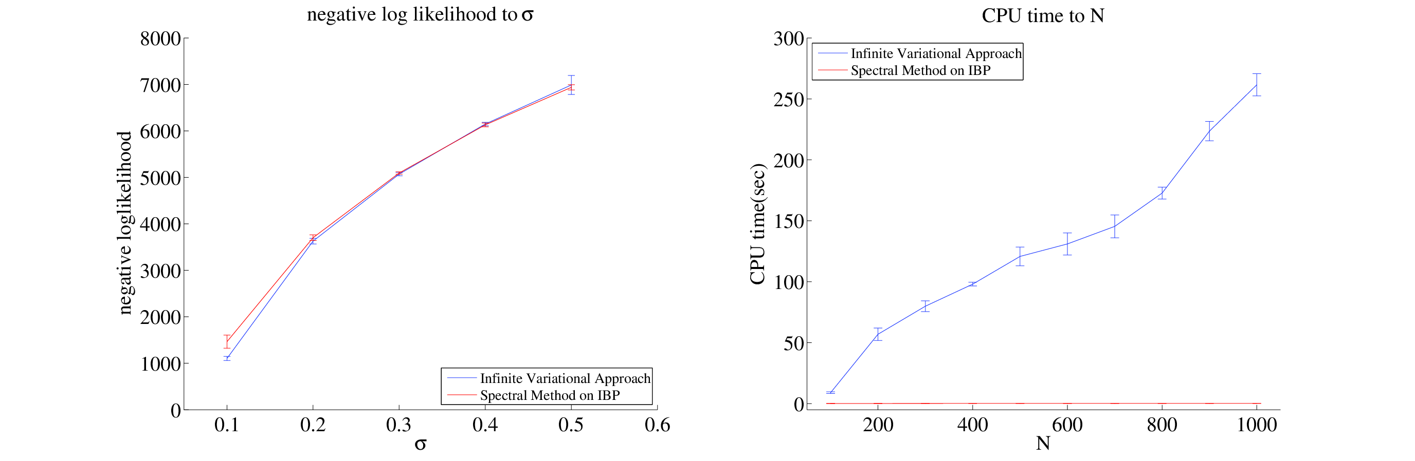
Figure 2: Comparison to infinite variational approach. The first plot compares the test negative log likelihood training on $N=500$ samples with different $\sigma$. The second plot shows the CPU time to data size, $N$, between the two methods.

Image Source Recovery

We repeated the same test using $100$ photos from Griffiths and Ghahramani (2011). We first reduce dimensionality on the data set by representing the images with 100 principal components and apply our algorithm on the 100-dimensional dataset (see Algorithm 1 for details). Figure 3 shows the result. We used $10$ initial iterations $50$ random seeds and $30$ final iterations $50$ in the Robust Power Tensor Method. The total runtime was $0.3$s on an intel Core i7 processor (3.2GHz).

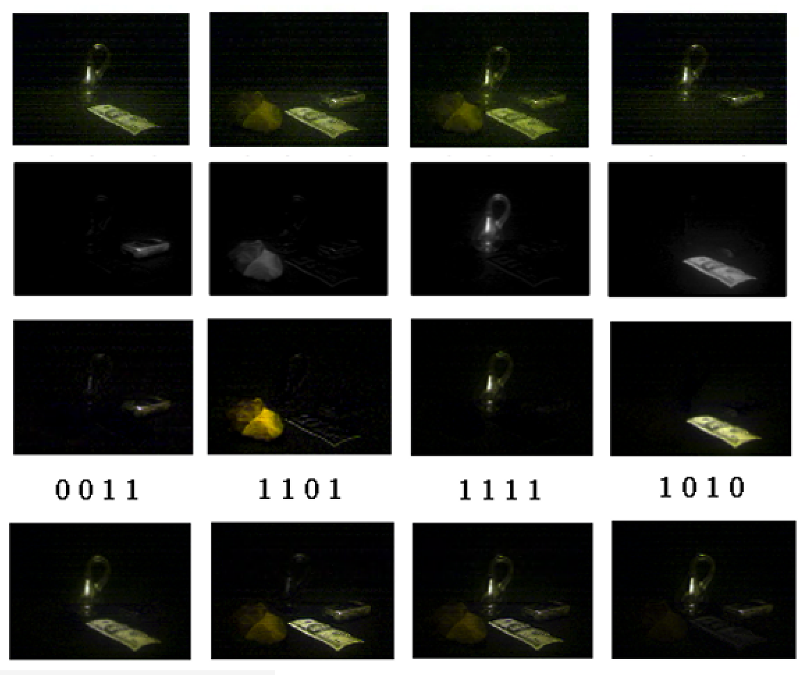
Figure 3: Results of modeling 100 images from Griffiths and Ghahramani (2011) of size $240\times 320$ by model (2). Row 1: four sample images containing up to four objects ($20 bill, Klein bottle, prehistoric handaxe, cellular phone). An object basically appears in the same location, but some small variation noise is generated because the items are put into scene by hand; Row 2: Independent attributes, as determined by infinite variational inference of Doshi et al. (2009) (note, the results in Griffiths and Ghahramani (2011) are black and white only); Row 3: Independent attributes, as determined by spectral IBP; Row 4: Reconstruction of the images via spectral IBP. The binary superscripts indicate the items identified in the image.

Gene Expression Data

As a first sanity check of the feasibility of our model for (3), we generated synthetic data using $x\in\mathbb{R}^{7}$ with $k=4$ sources and $n=500$ samples, as shown in Figure 5.

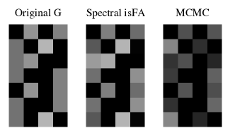
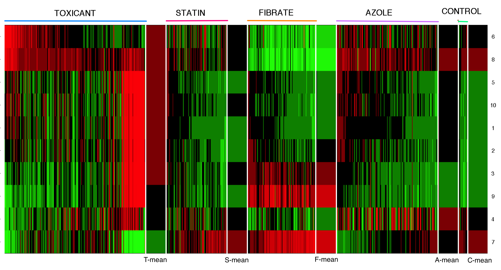
Figure 4: Recovery of the source matrix $A$ in model (3) when comparing MCMC sampling and spectral methods. MCMC sampling required $1.72$ seconds and yielded a Frobenius distance $\left\|A-A_{\mathrm{MCM}}\right\|_{F}=0.77$. Our spectral algorithm required $0.77$ seconds to achieve a distance $\left\|A-A_{\mathrm{Spectral}}\right\|_{F}=0.31$.

Figure 5: Gene signatures derived by the spectral IBP. They show that there are common hidden causes in the observed expression levels, thus offering a considerably simplified representation.

For a more realistic analysis we used a microarray dataset. The data consisted of 587 mouse liver samples detecting 8565 gene probes, available as dataset GSE2187 as part of NCBI’s Gene Expression Omnibus www.ncbi.nlm.nih.gov/geo. There are four main types of treatments, including Toxicant, Statin, Fibrate and Azole. Figure 5 shows the inferred latent factors arising from expression levels of samples on 10 derived gene signatures. According to the result, the group of fibrate-induced samples and a small group of toxicant-induced samples can be classified accurately by the special patterns. Azole-induced samples have strong positive signals on gene signatures 4 and 8, while statin-induced samples have strong positive signals only on the 9 gene signatures.

6.2 HDP

An attractive application of HDP is topic modelling in a corpus where in documents are grouped naturally. We use the Enron email corpus (Klimt and Yang, 2004) and the Multi-Domain Sentiment Dataset (Blitzer et al., 2007) to validate our algorithm. After the usual cleaning steps (stop word removal, numbers, infrequent words), our training dataset for Enron consisted of $167,851$ emails sent with $10,000$ vocabulary size and average $91$ words in each email. Among these, $126,697$ emails are sent internally within Enron and $41154$ are from external sources. In order to show that the topics are able to cover topics from external and internal sources and are not biased toward the larger group, we have $537$ internal emails and $4,63$ external email in our test data. To evaluate the computational efficiency of the spectral algorithms using fast count sketch tensor decomposition(FC) (Wang et al., 2015), robust tensor method (RB) and alternating least square (ALS), we compare the CPU time and per-word likelihood among these approaches.

Table 1: Results on Enron dataset with different tree structures and different solvers: spectral method for the HDP using fast count sketch method (sketch length is set to $10$), alternating least square (ALS) and robust tensor power method (RB).

Tree	K		sHDP (FC)	sHDP (ALS)	sHDP (RB)
Enron 2-layer	50	like./time	8.09/67	7.86/119	7.86/2641
	100	like./time	8.16/104	7.82/668	7.82/5841
Enron 3-layer	50	like./time	7.93/68	7.78/121	7.77/2710
	100	like./time	8.18/101	7.69/852	7.68/5782

We further compare spectral method under balanced/unbalanced tree structure of data on Multi-Domain Sentiment Dataset. The dataset contains reviews from Amazon reviews that fall into four categories: books, DVD, electronics and kitchen. We generate $2$ training datasets where one has balanced number of reviews under each categories (1900 reviews for each category) and the other has highly unbalanced number of examples at the leaf node (1900/1500/700/300 reviews for the four categories), while the test dataset consisted of 100 reviews for each categories. The result in Table 2 show that spectral algorithm with multi-layers structure will perform even better than with flat model when the tree structure is unbalanced.

Table 2: Results on Multi-Domain Sentimental dataset. Train data 1 is selected so that the there are balanced numbers of reviews under each category. Train data 2 is selected to have highly unbalanced child number at the leaf nodes.

Tree	train data 1	K=50	K=100	train data 2	K=50	k= 100
Sentiment 2-layer	like./time	7.9/38	7.99/151	like./time	8.23/36	8.14/147
Sentiment 3-layer	like./time	7.92/37	7.96/150	like./time	8.17/38	8.07.148

The results of the experiments throw light on two key points. First, leveraging the information in the form of hierarchical structure of documents, instead of blinding grouping the documents into a single-layer model like LDA, will result in better performance (i.e. higher log-likelihood) under different settings. The tree structure is able to eliminate the pernicious effects caused by unbalanced data. For example, a 2-layer model like LDA considers every email to be equally important, and so for a topic related to external events it will perform worse, as most of the emails are exchanged within the company and they are unlikely to possess topics related to the external emails. Second, although spectral method cannot obtain a solution that has higher performance in perplexity, it can be used as a tool for picking up a nice initial point.

7 Conclusion

The IBP and the HDP mixture models are useful and most popular nonparametric Bayesian tool. Unfortunately the computational complexity of the inference algorithms is high. Thus we propose a spectral algorithm to alleviate the pain. We first derived the low-order moments for both mixture model, and then described the algorithm to recover the latent factors of interest. Concentration of measure for this method is also provided. We demonstrate the advantages of utilizing structure information. High performance numerical linear algebra and more advanced optimization algorithms will improve matters further.

Acknowledgments

We would like to acknowledge support for this project from Oracle and Microsoft.

A Proof of Symmetric Tensors

Symmetric Tensors for the HDP
We begin our analysis by deriving the moments for a three layer HDP. This allows us to provide detail without being hampered by cumbersome notation. After that, we analyze the general expansion.

A.1 Three Layers

The three layer HDP is structurally similar to LDA. Its tensors are derived in Anandkumar et al. (2012a). We begin by considering a three model to gain intuition of how to obtain the general format of the tensors. The goal is to reconstruct the latent factors in $\Phi$. In the case of topic modeling, the $j$-th column denotes the word distribution of the $j$-th topic.

Lemma 11 (Symmetric tensors of $3$-layer HDP)

Given a $3$-layer HDP with hyperparameters $\gamma_{1}$ and $\gamma_{2}$ at layers $1$ and $2$ respectively, the symmetric tensors are given by

$$S_{1} :=M_{1}=T(\pi_{0},\Phi),$$

$$S_{2} :=M_{2}-C_{2}S_{1}S_{1}^{T}=M_{2}-\frac{\gamma_{2}\gamma_{1}}{\left(\gamma_{2}+1\right)\left(\gamma_{1}+1\right)}S_{1}S_{1}^{T}=T\left(C_{3}\cdot\mathrm{diag}\left(\pi_{0}\right),\Phi,\Phi\right),$$

$$S_{3} :=M_{3}-C_{4}\cdot S_{1}\otimes S_{1}\otimes S_{1}-C_{5}\cdot\mathfrak{S}_{3}\left[S_{2}\otimes M_{1}\right]=T\left(C_{6}\cdot\mathrm{diag}\left(\pi_{0}\right),\Phi,\Phi,\Phi\right),$$

where

$$C_{3} =\frac{\gamma_{2}+\gamma_{1}+1}{\left(\gamma_{1}+1\right)\left(\gamma_{2}+1\right)},$$

$$C_{4} =\frac{\gamma_{1}^{2}\gamma_{2}^{2}}{\left(\gamma_{1}+1\right)\left(\gamma_{1}+2\right)\left(\gamma_{2}+1\right)\left(\gamma_{2}+2\right)},$$

$$C_{5} =\frac{\gamma_{2}\gamma_{1}\left(\gamma_{1}+\gamma_{2}+2\right)}{\left(\gamma_{1}+2\right)\left(\gamma_{2}+2\right)\left(\gamma_{1}+\gamma_{2}+1\right)},$$

$$C_{6} =\frac{6\gamma_{1}+6\gamma_{2}+2\gamma_{1}^{2}+2\gamma_{2}^{2}+3\gamma_{2}\gamma_{1}+4}{\left(\gamma_{1}+1\right)\left(\gamma_{1}+2\right)\left(\gamma_{2}+1\right)\left(\gamma_{2}+2\right)}.$$

Proof.

By definition of the Dirichlet Process, the means match that of the reference measure. This means that we can integrate over the hierarchy

$$\mathbf{E}[x] =\mathbf{E}_{G_{p({\bf i})}|G_{p(p({\bf i}))},\gamma(p({\bf i}))}\left[\mathbf{E}_{x|G_{p({\bf i})},\gamma({\bf i})}\left[\Phi\pi_{{\bf i}}\right]\right]$$ (65)

$$=\mathbf{E}_{G_{p({\bf i})}|G_{p(p({\bf i}))},\gamma(p({\bf i}))}\left[\Phi\pi_{p(i)}\right]$$ (66)

$$=\Phi\pi_{p(p({\bf i}))}=\Phi\pi_{0}$$ (67)

Then deriving the first-order tensor is straightforward,

$$S_{1} :=M_{1}=\mathbf{E}_{x}\left[x_{1}\right]=\Phi\pi_{0}=T(\pi_{0},\Phi)$$ (68)

Similarly, to derive the second order tensor, we first need the following terms: for $i\neq j$ we have

$$\mathbf{E}_{G_{p({\bf i})}|G_{p(p({\bf i}))},\gamma(p({\bf i}))}\left[\mathbf{E}_{x|G_{p({\bf i})},\gamma({\bf i})}\left[\Phi_{i}\pi_{{\bf i}i}\pi_{{\bf i}j}^{T}\Phi_{j}^{T}\right]\right] =\mathbf{E}_{G_{p({\bf i})}|G_{p(p({\bf i}))},\gamma(p({\bf i}))}\left[\Phi_{i}\frac{\gamma_{2}\pi_{p({\bf i})i}\pi_{p({\bf i})j}^{T}}{\gamma_{2}+1}\Phi_{j}^{T}\right]$$ (69)

$$=T\left(\frac{\gamma_{2}}{\gamma_{2}+1}\frac{\gamma_{1}\pi_{0i}\pi_{0j}}{\gamma_{1}+1},\Phi_{i},\Phi_{j}\right)$$ (70)

Likewise, when the indices match, we obtain

$$\mathbf{E}_{G_{p({\bf i})}|G_{p(p({\bf i}))},\gamma(p({\bf i}))}\left[\mathbf{E}_{x|G_{p({\bf i})},\gamma({\bf i})}\left[\Phi_{i}\pi_{{\bf i}i}\pi_{{\bf i}i}^{T}\Phi_{i}^{T}\right]\right]$$ (71)

$$=\mathbf{E}_{G_{p({\bf i})}|G_{p(p({\bf i}))},\gamma(p({\bf i}))}\left[\Phi_{i}\frac{(\gamma_{2}\pi_{p({\bf i})i}+1)\pi_{p({\bf i})i}}{(\gamma_{2}+1)}\Phi_{i}^{T}\right]$$ (72)

$$=T\left(\frac{\gamma_{2}}{\left(\gamma_{2}+1\right)}\frac{\gamma_{1}\pi_{0i}^{2}+\pi_{0i}}{\left(\gamma_{1}+1\right)}+\frac{1}{\left(\gamma_{2}+1\right)}\pi_{0i},\Phi_{i},\Phi_{i}\right)$$ (73)

Then the moment $M_{2}$ could be written as

$$M_{2}= \mathbf{E}_{x}\left[x_{1}\otimes x_{2}\right]$$ (74)

$$= \mathbf{E}\left[\mathbf{E}_{x}\left[x_{1}\otimes x_{2}|G_{{\bf i}}\right]\right]$$ (75)

$$= \mathbf{E}\left[\mathbf{E}_{x}\left[x_{1}|G_{{\bf i}}\right]\otimes\mathbf{E}_{x}\left[x_{2}|G_{{\bf i}}\right]\right]$$ (76)

$$= \Phi\mathbf{E}\left[\mathbf{E}\left[\pi_{{\bf i}}\pi_{{\bf i}}^{T}\right]\right]\Phi^{T}$$ (77)

$$= \frac{\gamma_{2}\gamma_{1}}{\left(\gamma_{2}+1\right)\left(\gamma_{1}+1\right)}S_{1}\otimes S_{1}+T\left(\frac{\gamma_{2}+\gamma_{1}+1}{\left(\gamma_{1}+1\right)\left(\gamma_{2}+1\right)}\cdot\mathrm{diag}\left(\pi_{0}\right),\Phi,\Phi\right)$$ (78)

The second-order symmetric tensor $S_{2}$ could then be obtained by defining

$$S_{2} :=M_{2}-\frac{\gamma_{2}\gamma_{1}}{\left(\gamma_{2}+1\right)\left(\gamma_{1}+1\right)}S_{1}\otimes S_{1}=T\left(\frac{\gamma_{2}+\gamma_{1}+1}{\gamma_{1}\left(\gamma_{1}+1\right)\left(\gamma_{2}+1\right)}\cdot\mathrm{diag}\left(G_{0}\right),\Phi,\Phi\right).$$ (79)

Before deriving the third-order tensor, we derive $\mathbf{E}[(\Phi_{i}\pi_{{\bf i}i})\otimes(\Phi_{j}\pi_{{\bf i}j})\otimes(\Phi_{j}\pi_{{\bf i}j})]$ for the following three cases. First, for $i=j=k,$ we have:

$$\mathbf{E}_{G_{p({\bf i})}|G_{p(p({\bf i}))},\gamma(p({\bf i}))}\left[\mathbf{E}_{x|G_{p({\bf i})},\gamma({\bf i})}\left[(\Phi_{i}\pi_{{\bf i}i})^{\otimes 3}\right]\right]$$ (80)

$$=\mathbf{E}\left[T(\frac{\pi_{p({\bf i})i}\left(\gamma_{2}\pi_{p({\bf i})i}+1\right)\left(\gamma_{2}\pi_{p({\bf i})i}+2\right)}{\left(\gamma_{2}+1\right)\left(\gamma_{2}+2\right)},\Phi_{i},\Phi_{i},\Phi_{i})\right]$$

$$=T\bigg{(}\frac{\gamma_{2}^{2}}{\left(\gamma_{2}+1\right)\left(\gamma_{2}+2\right)}\frac{\pi_{0i}\left(\gamma_{1}\pi_{0i}+1\right)\left(\gamma_{1}\pi_{0i}+2\right)}{\left(\gamma_{1}+1\right)\left(\gamma_{1}+2\right)}+\frac{3\gamma_{2}}{\left(\gamma_{2}+1\right)\left(\gamma_{2}+2\right)}\frac{\pi_{0i}\left(\gamma_{1}\pi_{0i}+1\right)}{\left(\gamma_{1}+1\right)}$$

$$\,\,\,\,\,\,\,\,\,\,\,\,\,\,\,\,\,\,\,\,\,+\frac{2\pi_{0i}}{\left(\gamma_{2}+1\right)\left(\gamma_{2}+2\right)},\Phi_{i},\Phi_{i},\Phi_{i}\bigg{)}$$

Second, for $i=j\neq k,$ we have:

$$\mathbf{E}_{G_{p({\bf i})}|G_{p(p({\bf i}))},\gamma(p({\bf i}))}\left[\mathbf{E}_{x|G_{p({\bf i})},\gamma({\bf i})}\left[(\Phi_{i}\pi_{{\bf i}i})^{\otimes 2}\otimes(\Phi_{k}\pi_{{\bf i}k})\right]\right]$$ (81)

$$=\mathbf{E}\left[T\bigg{(}\frac{\pi_{p({\bf i})i}\left(\gamma_{2}\pi_{p({\bf i})i}+1\right)\gamma_{2}\pi_{p({\bf i})k}}{\left(\gamma_{2}+1\right)\left(\gamma_{2}+2\right)},\Phi_{i},\Phi_{i},\Phi_{k}\bigg{)}\right]$$

$$=T\bigg{(}\frac{\gamma_{2}^{2}}{\left(\gamma_{2}+1\right)\left(\gamma_{2}+2\right)}\frac{\pi_{0i}\left(\gamma_{1}\pi_{0i}+1\right)\gamma_{1}\pi_{0k}}{\left(\gamma_{1}+1\right)\left(\gamma_{1}+2\right)}+\frac{\gamma_{2}}{\left(\gamma_{2}+1\right)\left(\gamma_{2}+2\right)}\frac{\gamma_{1}\pi_{0i}\pi_{0k}}{\left(\gamma_{1}+1\right)},\Phi_{i},\Phi_{i},\Phi_{k}\bigg{)}$$

Third, for $i\neq j\neq k,$ we have:

$$\mathbf{E}\left[\mathbf{E}_{x|G_{p({\bf i})},\gamma({\bf i})}\left[(\Phi_{i}\pi_{{\bf i}i})\otimes(\Phi_{j}\pi_{{\bf i}j})\otimes(\Phi_{k}\pi_{{\bf i}k})\right]\right]$$ (82)

$$=\mathbf{E}\left[T\bigg{(}\frac{\gamma_{2}^{2}\pi_{p({\bf i})i}\pi_{p({\bf i})j}\pi_{p({\bf i})k}}{\left(\gamma_{2}+1\right)\left(\gamma_{2}+2\right)},\Phi_{i},\Phi_{j},\Phi_{k}\bigg{)}\right]$$ (83)

$$=T\bigg{(}\frac{\gamma_{2}^{2}}{\left(\gamma_{2}+1\right)\left(\gamma_{2}+2\right)}\frac{\gamma_{1}^{2}\pi_{0i}\pi_{0j}\pi_{0k}}{\left(\gamma_{1}+1\right)\left(\gamma_{1}+2\right)},\Phi_{i},\Phi_{j},\Phi_{k}\bigg{)}.$$ (84)

Defining

$$S_{3} :=M_{3}-C_{4}\cdot S_{1}\otimes S_{1}\otimes S_{1}-C_{5}\cdot\mathfrak{S}_{3}\left[S_{2}\otimes M_{1}\right]$$ (85)

$$=T\left(C_{6}\cdot\mathrm{diag}\left(\pi_{0}\right),\Phi,\Phi,\Phi\right)$$ (86)

we solve $C_{4},C_{5},C_{6}$ as follows.

Note that for $i\neq j\neq k,$ $[S_{3}]_{ijk}=0$ and $\left[\mathfrak{S}_{3}[S_{2}\otimes M_{1}]\right]_{ijk}=0$. Thus

$$C_{4} =\frac{[M_{3}]_{ijk}}{[S_{1}]_{i}[S_{1}]_{j}[S_{1}]_{k}}$$ (87)

$$=\frac{\gamma_{2}^{2}}{\left(\gamma_{2}+1\right)\left(\gamma_{2}+2\right)}\frac{\gamma_{1}^{2}\pi_{0i}\pi_{0j}\pi_{0k}}{\left(\gamma_{1}+1\right)\left(\gamma_{1}+2\right)}\cdot\frac{1}{\pi_{0i}\pi_{0j}\pi_{0k}}$$ (88)

$$=\frac{\gamma_{2}^{2}\gamma_{1}^{2}}{\left(\gamma_{2}+1\right)\left(\gamma_{2}+2\right)\left(\gamma_{1}+1\right)\left(\gamma_{1}+2\right)}$$ (89)

Similarly, for $i=j\neq k,$ $[S_{3}]_{ijk}=0$. Thus

$$C_{5} =\frac{[M_{3}]_{iik}-C_{4}[S_{1}]_{i}[S_{1}]_{i}[S_{1}]_{k}}{[S_{2}]_{ii}[{M_{1}}]_{k}}$$ (90)

$$= \frac{\gamma_{2}^{2}\gamma_{1}\pi_{0i}\pi_{0k}+\gamma_{2}\left(\gamma_{1}+2\right)\gamma_{1}\pi_{0i}\pi_{0k}}{\left(\gamma_{2}+1\right)\left(\gamma_{2}+2\right)\left(\gamma_{1}+1\right)\left(\gamma_{1}+2\right)}\cdot\frac{\left(\gamma_{1}+1\right)\left(\gamma_{2}+1\right)}{\pi_{0i}\pi_{0k}\left(\gamma_{2}+\gamma_{1}+1\right)}$$ (91)

$$= \frac{\gamma_{2}\gamma_{1}\left(\gamma_{1}+\gamma_{2}+2\right)}{\left(\gamma_{1}+2\right)\left(\gamma_{2}+2\right)\left(\gamma_{1}+\gamma_{2}+1\right)}$$ (92)

Finally,

$$C_{6} =\frac{[M_{3}]_{iii}-C_{4}[S_{1}]_{i}[S_{1}]_{i}[S_{1}]_{i}-3C_{5}[S_{2}]_{ii}[M_{1}]_{i}}{\gamma_{i}}$$

$$=\frac{2\gamma_{2}^{2}\pi_{0i}+3\gamma_{2}\left(\gamma_{1}+2\right)\pi_{0i}+2\left(\gamma_{1}+1\right)\left(\gamma_{1}+2\right)\pi_{0i}}{\left(\gamma_{2}+1\right)\left(\gamma_{2}+2\right)\left(\gamma_{1}+1\right)\left(\gamma_{1}+2\right)\gamma_{1}\pi_{0i}}$$

$$=\frac{6\gamma_{1}+6\gamma_{2}+2\gamma_{1}^{2}+2\gamma_{2}^{2}+3\gamma_{2}\gamma_{1}+4}{\gamma_{1}\left(\gamma_{1}+1\right)\left(\gamma_{1}+2\right)\left(\gamma_{2}+1\right)\left(\gamma_{2}+2\right)}$$ (93)

∎

A.2 Multiple Layer HDP

Lemma 12 (Symmetric Tensors of HDP)

For an $L$-level HDP, with hyperparameters, $\gamma_{1},\gamma_{2}$, …$\gamma_{L-1}$ we have

$$S_{1} :=M_{1}=T(\pi_{0},\Phi),$$

$$S_{2} :=M_{2}-C_{2}\cdot S_{1}S_{1}^{T}=T(C_{3}\cdot\mathrm{diag}\left(\pi_{0}\right),\Phi,\Phi),$$

$$S_{3} :=M_{3}-C_{4}\cdot S_{1}\otimes S_{1}\otimes S_{1}-C_{5}\cdot\mathfrak{S}_{3}\left[S_{2}\otimes M_{1}\right]=T(C_{6}\cdot\mathrm{diag}\left(\pi_{0}\right),\Phi,\Phi,\Phi),$$

The key difference is that here the coefficients $C_{i}$ are recursively defined since we need to take expectations all the way up to the root node. This yields

$$C_{2}= \frac{\prod\limits_{i=1}^{L-1}\gamma_{i}}{\prod\limits_{i=1}^{L-1}\left(\gamma_{i}+1\right)},\,\,\,\,\,\,\,C_{3}=\sum\limits_{i=1}^{L-1}\frac{\prod\limits_{j=1}^{i-1}\gamma_{L-j}}{\prod\limits_{j=1}^{i}\left(\gamma_{L-j}+1\right)};$$

$$C_{4}= \frac{\prod\limits_{i=1}^{L-1}{\gamma_{i}}^{2}}{\prod\limits_{i=1}^{L-1}\left(\left(\gamma_{i}+1\right)\left(\gamma_{i}+2\right)\right)},\,\,\,\,\,\,C_{5}=\sum\limits_{i=1}^{L-1}\frac{\prod\limits_{j=1}^{i-1}{\gamma_{L-j}}\prod\limits_{j=1}^{L-1}\gamma_{j}}{\prod\limits_{j=1}^{i}\left(\gamma_{L-j}+2\right)\prod\limits_{j=1}^{L-1}\left(\gamma_{j}+1\right)}/C_{3}$$

$$C_{6}= 3\sum\limits_{i=1}^{L-2}\sum\limits_{j=i+1}^{L}\frac{\prod\limits_{k=1}^{i-1}\gamma_{L-k}\prod\limits_{k=1}^{j-1}\gamma_{L-k}}{\prod\limits_{k=1}^{i}\left(\gamma_{L-k}+2\right)\prod\limits_{k=1}^{j}\left(\gamma_{L-k}+1\right)}+2\sum\limits_{i=1}^{L-1}\frac{\prod\limits_{j=1}^{i-1}{\gamma_{L-j}}^{2}}{\prod\limits_{j=1}^{i}\left(\left(\gamma_{L-j}+1\right)\left(\gamma_{L-j}+2\right)\right)}$$

B Proof of reconstruction formula for the spectral HDP

B.1 Proof of reconstruction formula

For simplicity in the proof, in Equation (19) (20) (21), we define the diagonal coefficients for $S_{i}$ to be $C_{i}\in\mathbb{R}^{K}$, i.e., $C_{2}=\pi-\pi^{2}$, $C_{3}=\pi-3\pi^{2}+2\pi^{3}$ and $C_{4}=\pi-7\pi^{2}+12\pi^{3}-6\pi^{4}$, so that

$$S_{2} =T(\mathrm{diag}\left(C_{2}\right),\Phi,\Phi),\;\;\;S_{3}=T(\mathrm{diag}\left(C_{3}\right),\Phi,\Phi,\Phi),\;\;\;S_{4}=T(\mathrm{diag}\left(C_{4}\right),\Phi,\Phi,\Phi,\Phi).$$

Following step 6 in Algorithm 1, we obtain whitening matrix $W$ by doing svd on $S_{2}$. Suppose the svd of matrix $T(\mathrm{diag}\left(\sqrt{C_{2}}\right),\Phi)=U\Sigma^{1/2}V^{\top}$, we have $S_{2}=U\Sigma^{1/2}V^{\top}V\Sigma^{1/2}U^{\top}=USU^{T}$ and $W=U\Sigma^{-1/2}$. Using the fact that

$$S_{3}=T\left(\mathrm{diag}\left(C_{3}C_{2}^{-3/2}\right),\mathrm{diag}\left(\sqrt{C_{2}}\right)\Phi,\mathrm{diag}\left(\sqrt{C_{2}}\right)\Phi,\mathrm{diag}\left(\sqrt{C_{2}}\right)\Phi\right),$$

we have

$$W_{3} =T\left(S_{3},W,W,W\right)$$

$$=T\left(\mathrm{diag}\left(C_{3}C_{2}^{-3/2}\right),\Sigma^{-1/2}U^{\top}(U\Sigma^{1/2}V^{\top}),\Sigma^{-1/2}U^{\top}(U\Sigma^{1/2}V^{\top}),\Sigma^{-1/2}U^{\top}(U\Sigma^{1/2}V^{\top})\right)$$

$$=T\left(\mathrm{diag}\left(C_{3}C_{2}^{-3/2}\right),V^{\top},V^{\top},V^{\top}\right).$$ (94)

The diagonalized tensor $W_{3}$, with some permutation $\tau$ on $[K]$ and $s_{i}\in\left\{\pm 1\right\}$, has eigenvalues and eigenvectors:

$$\lambda_{i} =s_{i}C_{3,i}C_{2,i}^{-3/2},\,\,\,v_{i}=s_{i}(V^{\top}),e_{\tau\left(i\right)},$$ (95)

where $C_{i,j}$ representing the $j$-th element in $C_{i}$. After obtaining $v_{i}$, we multiply $v_{i}$ by $(W^{{\dagger}})^{\top}$ to rotate it back to $\Phi_{i}$ as describing in step 15 in Algorithm 1, where $W^{{\dagger}}=(W^{\top}W)^{-1}W^{\top}=\Sigma^{1/2}U^{\top}$, we get

$$(W^{{\dagger}})^{\top}v_{i} =s_{i}U\Sigma^{1/2}V^{\top}e_{\tau\left(i\right)}=s_{i}T(\mathrm{diag}\left(\sqrt{C_{2}}\right),\Phi)e_{\tau\left(i\right)}=s_{i}\sqrt{C_{2,i}}\Phi_{\tau\left(i\right)},$$ (96)

which yields $\Phi_{\tau\left(i\right)}=\frac{(W^{{\dagger}})^{\top}v_{i}}{s_{i}\sqrt{C_{2,i}}}$. With the fact that $s_{i}=C_{3,i}C_{2,i}^{-3/2}\lambda_{i}^{-1}$ from Equation (95), we have

$$\Phi_{\tau\left(i\right)} =\frac{\lambda_{i}}{\left(C_{3,i}C_{2,i}^{-1}\right)}(W^{{\dagger}})^{\top}v_{i}=C_{2,i}^{-1/2}(W^{{\dagger}})^{\top}v_{i}.$$ (97)

Plug in the definition of $C_{2}$, we get the scale factor for $i\in[K_{1}]$. For $\Phi_{i}$ which are recovered by conducting tensor decomposition on $W_{4}$, we first examine

$$W_{4}=T\left(S_{4},W,W,W,W\right) =T\left(\mathrm{diag}\left(C_{4,i}C_{2,i}^{-2}\right),V^{\top},V^{\top},V^{\top},V^{\top}\right),$$ (98)

and obtain

$$\lambda_{i} =C_{4,i}C_{2,i}^{-2},\,\,\,v_{i}=s_{i}(V^{\top})e_{\tau\left(i\right)}.$$ (99)

By using the fact that $s_{i}=s_{i}C_{4,i}C_{2,i}^{-2}{\lambda_{i}}^{-1}$ and Equation (96), we have

$$\Phi_{\tau\left(i\right)} =\frac{(W^{{\dagger}})^{\top}v_{i}}{s_{i}\sqrt{C_{2,i}}}=\frac{s_{i}}{\left(C_{4,i}C_{2,i}^{-3/2}\right)\lambda_{i}^{-1}}=s_{i}(W^{{\dagger}})^{\top}v_{i}=s_{i}C_{2,i}^{-1/2}(W^{{\dagger}})^{\top}v_{i},\,\,\,\,\forall i\in\left[K_{1}+1,\cdots,K\right].$$ (100)

Note that the value of $\pi_{i}$ used to construct $C_{j}$ can be recovered by Equation (95) and (99) after obtaining $\lambda_{i}$.

B.2 Proof of reconstruction formula for the spectral HDP

Using the results in the previous section, the corresponding eigenvalues $\lambda_{i}$ and eigenvectors $v_{i}$, with some permutation ${\bf\pi}$, are

$$\lambda_{i} =s_{i}\frac{C_{6}}{C_{3}\sqrt{C_{3}}}\mathrm{diag}\left(\frac{1}{\sqrt{\gamma_{\pi_{i}}}}\right),\,\,v_{i}=s_{i}V^{T}e_{\pi_{i}}$$ (101)

Therefore

$$W^{+} =\left(W^{T}W\right)^{-1}W^{T}=SU^{T}$$ (102)

$$\left(W^{+}\right)^{T}v_{i} =s_{i}(US)V^{T}e_{\pi_{i}}=s_{i}\sqrt{C_{3}}\sqrt{\gamma_{\pi_{i}}}\Phi_{\pi_{i}}$$ (103)

$$\Phi_{\pi_{i}} =\frac{\left(W^{+}\right)^{T}v_{i}}{s_{i}\sqrt{C_{3}}\sqrt{\gamma_{\pi_{i}}}}$$ (104)

Rearranging Equation 101, we have

$$s_{i} =\frac{C_{6}}{C_{3}\sqrt{C_{3}}\sqrt{\gamma_{\pi_{i}}}\lambda_{i}};\,\,\,\,\,\Phi_{\pi_{i}}=\frac{\lambda_{i}(W^{+})^{T}v_{i}}{C_{6}/C_{3}}$$ (105)

C Proof of Lemma 5

Proof.

Here we only show the derivation of the fourth-order conditional moments. The other inequalities can be found in Hsu and Kakade (2012). Under the stated model, the fourth-order conditional moment can be expended as

$$M_{4,z_{i}} =M_{1,z_{i}}\otimes M_{1,z_{i}}\otimes M_{1,z_{i}}\otimes M_{1,z_{i}}+\sigma^{2}\mathfrak{S}_{6}\left[M_{1,z_{i}}\otimes M_{1,z_{i}}\otimes\mathbf{1}\right]+\mathbf{E}\left[\epsilon\otimes\epsilon\otimes\epsilon\otimes\epsilon\right],$$

which yields

$$\hat{M}_{4,z_{i}}-M_{4,z_{i}}$$

$$=\frac{1}{\hat{w}_{z_{i}}n}\bigg{(}\sum\limits_{x\in B_{z_{i}}}\left(x_{j}-M_{1,z_{i}}\right)\otimes\left(x_{j}-M_{1,z_{i}}\right)\otimes\left(x_{j}-M_{1,z_{i}}\right)\otimes\left(x_{j}-M_{1,z_{i}}\right)-\sigma^{4}\mathfrak{S}_{3}\left[\mathbf{1}\otimes\mathbf{1}\right]$$

$$\,\,\,\,\,\,+\sum\limits_{x\in B_{z_{i}}}\left(\mathfrak{S}_{4}\left[M_{1,z_{i}}\otimes\left(x_{j}-M_{1,z_{i}}\right)\otimes\left(x_{j}-M_{1,z_{i}}\right)\otimes\left(x_{j}-M_{1,z_{i}}\right)\right]\right)$$

$$\,\,\,\,\,\,+\sum\limits_{x\in B_{z_{i}}}\left(\mathfrak{S}_{6}\left[M_{1,z_{i}}\otimes M_{1,z_{i}}\otimes\left(\left(x_{j}-M_{1,z_{i}}\right)\otimes\left(x_{j}-M_{1,z_{i}}\right)-\sigma^{2}\mathbf{1}\right)\right]\right)$$

$$\,\,\,\,\,\,+\sum\limits_{x\in B_{z_{i}}}\mathfrak{S}_{4}\left[M_{4,z_{i}}\otimes M_{4,z_{i}}\otimes M_{4,z_{i}}\otimes\left(x_{j}-M_{1,z_{i}}\right)\right]\bigg{)}$$ (106)

Suppose $V=V_{1}\Sigma V_{2}^{\top}$ is the SVD of $V$, where $V_{1}\in\mathrm{R}^{d\times r}$ consists of orthonormal columns. With $y_{j,z_{i}}=V_{1}^{\top}\left(x_{j}-M_{1,z_{i}}\right)$, applying triangle inequalities to Equation (C) yields

$$\left\|T\left(\hat{M}_{4,z_{i}}-M_{4,z_{i}},V,V,V,V\right)\right\|_{2}$$

$$\leq\left\|V\right\|_{2}^{4}\left\|\frac{1}{\hat{w}_{z_{i}}n}\sum\limits_{x\in B_{z_{i}}}\left(y_{j,z_{i}}\otimes y_{j,z_{i}}\otimes y_{j,z_{i}}\otimes y_{j,z_{i}}-\sigma^{4}\mathfrak{S}_{3}\left[\mathbf{1}\otimes\mathbf{1}\right]\right)\right\|_{2}$$

$$\,\,\,\,\,\,+4\left\|V^{\top}M_{1,z_{i}}\right\|_{2}\left\|\frac{1}{\hat{w}_{z_{i}}n}\sum\limits_{x\in B_{z_{i}}}y_{j,z_{i}}\otimes y_{j,z_{i}}\otimes y_{j,z_{i}}\right\|_{2}$$

$$\,\,\,\,\,\,+6\left\|V^{\top}M_{1,z_{i}}\right\|_{2}^{2}\left\|\frac{1}{\hat{w}_{z_{i}}n}\sum\limits_{x\in B_{z_{i}}}\left(y_{j,z_{i}}\otimes y_{j,z_{i}}-\sigma^{2}\mathbf{1}\right)\right\|_{2}+4\left\|R^{\top}M_{1,z_{i}}\right\|_{2}^{3}\left\|\frac{1}{\hat{w}_{z_{i}}n}\sum\limits_{x\in B_{z_{i}}}y_{j,z_{i}}\right\|_{2},$$

By using Lemma 19, we bound the first term by

$$\Pr\Bigg{[} \left\|\frac{1}{\hat{w}_{z_{i}}n}\sum\limits_{x\in B_{z_{i}}}\left(y_{j,z_{i}}\otimes y_{j,z_{i}}\otimes y_{j,z_{i}}\otimes y_{j,z_{i}}-\mathbf{E}\left[\epsilon\otimes\epsilon\otimes\epsilon\otimes\epsilon\right]\right)\right\|_{2}$$

$$\,\,\,\,\,\,\,\,\,\,\,\,\,\,\,\,\,\,\,\,\,\,\,\,\,\,\,\,\,\,\,\,>\sigma^{4}\sqrt{\frac{8192\left(r\ln 17+\ln\left(2K/\delta\right)\right)^{2}}{n^{2}}+\frac{32\left(r\ln 17+\ln\left(2K/\delta\right)\right)^{3}}{n^{3}}}\Bigg{]}\leq\delta.$$ (107)

∎

D Concentration of Measure for the spectral IBP

In this section, we provides bounds for tensors of linear gaussian latent feature model. The concentration behavior is more complicated than that of the bounded moments in Theorem 3 due to the additive Gaussian noise. Here we restate the model as

$$x=\Phi z+\epsilon$$ (108)

where $x\in\mathbb{R}^{d}$ is the observation, $z\in\{0,1\}^{K}$ is a binary vector indicating the possession of certain latent vector and $\epsilon$ is gaussian noise drawn from $N(0,\sigma^{2}\mathbf{1})$. Using the results for bounded moments, we derive the concentration measure for tensors.

D.1 Estimation of $\sigma$, $S_{2}$, $S_{3}$, $S_{4}$

Note that we have $\sigma^{2}=\lambda_{min}\left[{M_{2}}-{M_{1}}\otimes{M_{1}}\right]=\varsigma_{K}{\left[{M_{2}}-{M_{1}}\otimes{M_{1}}\right]}$, where $\varsigma_{t}\left[M\right]$ denoting the $t-th$ singular value of matrix $M$ which is defined in Theorem 7. Here we define $\hat{S}_{2,K}$ to be the best rank $k$ approximation of $\hat{M_{2}}-\hat{M_{1}}\otimes\hat{M_{1}}-\hat{\sigma}^{2}\mathbf{1}$, which is the truncated matrix $S_{2}$ in Algorithm 1. $\hat{S}_{i}$ denotes the empirical tensors derived from summation of $\hat{M}_{i}$ and $\hat{\sigma}$. $S_{i}$ denotes the theoretical values.

Lemma 13

(Accuracy of $\sigma^{2}$, $\sigma^{4}$ and $M_{2,K}$)

$$\left|\hat{\sigma}^{2}-\sigma^{2}\right|\leq\left\|\hat{M}_{2}-M_{2}\right\|_{2}+\left\|\hat{M}_{1}-M_{1}\right\|_{2}^{2}+2\left\|\hat{M}_{1}-M_{1}\right\|_{2}\left\|M_{1}\right\|_{2}$$ (109)

$$\left|\hat{\sigma}^{4}-\sigma^{4}\right|\leq\left|\hat{\sigma}^{2}-\sigma^{2}\right|^{2}+2\sigma^{2}\left|\hat{\sigma}^{2}-\sigma^{2}\right|$$ (110)

$$\left\|\hat{S}_{2,k}-S_{2}\right\|_{2}\leq 4\left(\left\|\hat{M}_{2}-M_{2}\right\|_{2}+\left\|\hat{M_{1}}-M_{1}\right\|_{2}^{2}+2\left\|M_{1}\right\|_{2}\left\|\hat{M_{1}}-M_{1}\right\|_{2}\right)$$ (111)

Proof.

For the first order tensor, the inequality holds trivially due to the guarantees for $\left\|\hat{M}_{1}-M_{1}\right\|_{2}$. Next we bound the difference in variance estimates. Using the fact that differences in the $k$-th eigenvalues are bounded by the matrix norm of the difference we have that

$$\left|\hat{\sigma}^{2}-\sigma^{2}\right| =\left|\varsigma_{k}\left[\hat{M}_{2}-\hat{M}_{1}\otimes\hat{M}_{1}\right]-\varsigma_{k}{\left[{M_{2}}-{M_{1}}\otimes{M_{1}}\right]}\right|$$ (112)

$$\leq\left\|\left[\hat{M}_{2}-\hat{M}_{1}\otimes\hat{M}_{1}\right]-{\left[{M_{2}}-{M_{1}}\otimes{M_{1}}\right]}\right\|_{2}$$ (113)

$$\leq\left\|\hat{M}_{2}-M_{2}\right\|_{2}+\left\|\hat{M}_{1}-M_{1}\right\|_{2}^{2}+2\left\|\hat{M}_{1}-M_{1}\right\|_{2}\left\|M_{1}\right\|_{2}.$$ (114)

The second inequality follows the Weyl’s inequality and the last inequality is obtained by the triangle inequality. For estimation of $\hat{\sigma^{4}}$,

$$\left|\hat{\sigma}^{4}-\sigma^{4}\right|\leq\left|(\hat{\sigma}^{2}-\sigma^{2})^{2}+2\sigma^{2}(\hat{\sigma}^{2}-\sigma^{2})\right|\leq\left|\hat{\sigma}^{2}-\sigma^{2}\right|^{2}+2\sigma^{2}\left|\hat{\sigma}^{2}-\sigma^{2}\right|.$$ (115)

For the last claimed inequality, with Weyl’s inequality,

$$\left\|\hat{S}_{2,k}-\left(\hat{M_{2}}-\hat{M_{1}}\otimes\hat{M_{1}}-\hat{\sigma}^{2}\mathbf{1}\right)\right\|_{2}\leq\varsigma_{k+1}\left[\hat{M_{2}}-\hat{M_{1}}\otimes\hat{M_{1}}-\hat{\sigma}^{2}\mathbf{1}\right]$$ (116)

$$=\left\|\varsigma_{k+1}\left[\hat{M_{2}}-\hat{M_{1}}\otimes\hat{M_{1}}-\hat{\sigma}^{2}\mathbf{1}\right]-\varsigma_{k+1}\left[M_{2}-M_{1}\otimes M_{1}-\sigma^{2}\mathbf{1}\right]\right\|_{2}$$ (117)

$$\leq\left\|\hat{M_{2}}-\hat{M_{1}}\otimes\hat{M_{1}}-\hat{\sigma}^{2}\mathbf{1}-\left(M_{2}-M_{1}\otimes M_{1}-\sigma^{2}\mathbf{1}\right)\right\|_{2}$$ (118)

, which yields

$$\left\|\hat{S}_{2,k}-S_{2}\right\|_{2} \leq\left\|\hat{S}_{2,k}-\left(\hat{M_{2}}-\hat{M_{1}}\otimes\hat{M_{1}}-\hat{\sigma}^{2}\mathbf{1}\right)\right\|_{2}$$

$$\,\,\,\,\,\,+\left\|\hat{M_{2}}-\hat{M_{1}}\otimes\hat{M_{1}}-\hat{\sigma}^{2}\mathbf{1}-\left(M_{2}-M_{1}\otimes M_{1}-\sigma^{2}\mathbf{1}\right)\right\|_{2}$$ (119)

$$\leq 2\left(\left\|\hat{M}_{2}-M_{2}\right\|_{2}+\left\|\hat{M_{1}}-M_{1}\right\|_{2}^{2}+2\left\|M_{1}\right\|_{2}\left\|\hat{M_{1}}-M_{1}\right\|_{2}+\left|\hat{\sigma}^{2}-\sigma^{2}\right|\right)$$ (120)

$$\leq 4\left(\left\|\hat{M}_{2}-M_{2}\right\|_{2}+\left\|\hat{M_{1}}-M_{1}\right\|_{2}^{2}+2\left\|M_{1}\right\|_{2}\left\|\hat{M_{1}}-M_{1}\right\|_{2}\right).$$ (121)

∎

The inequalities for $\sigma$ can be used for bounding the tensors $S_{2}$, $S_{3}$ and $S_{4}$, which will be shown next, and the inequality for $S_{2,k}$ will be used in bounding whitened tensor in Section D.2.

Lemma 14

(Accuracy of $S_{2}$, $S_{3}$ and $S_{4}$) For a fixed matrix $V\in\mathbb{R}^{d\times K}$

$$\left\|T\left(\hat{S}_{2}-S_{2},V,V\right)\right\|_{2}\leq\left\|T\left(\hat{M}_{2}-M_{2},V,V\right)\right\|_{2}+\left\|T\left(\hat{M}_{1}-M_{1},V\right)\right\|_{2}^{2}$$

$$\,\,\,\,\,\,\,\,\,\,\,\,\,\,\,\,\,\,\,\,\,\,\,\,\,\,\,\,\,\,\,\,\,\,\,\,\,\,\,\,\,\,\,\,\,\,\,\,\,\,\,\,\,\,\,\,\,\,\,\,\,\,\,+2\left\|T\left(M_{1},V\right)\right\|_{2}\left\|T\left(\hat{M}_{1}-M_{1},V\right)\right\|_{2}+\left\|V\right\|_{2}^{2}\left|\hat{\sigma}^{2}-\sigma^{2}\right|$$ (122)

$$\left\|T\left(\hat{S}_{3}-S_{3},V,V,V\right)\right\|_{2}$$

$$\leq\left\|T\left(\hat{M}_{3}-M_{3},V,V,V\right)\right\|_{2}+\left(\left\|T\left(\hat{M}_{1}-M_{1},V\right)\right\|_{2}+\left\|T\left(M_{1},V\right)\right\|_{2}\right)^{3}-\left\|T\left(M_{1},V\right)\right\|_{2}^{3}$$

$$\,\,\,\,\,\,+3\bigg{(}\left\|T\left(\hat{M}_{1}-M_{1},V\right)\right\|_{2}\left\|T\left(\hat{S}_{2}-S_{2},V,V\right)\right\|_{2}+\left\|T\left(M_{1},V\right)\right\|_{2}\left\|T\left(\hat{S}_{2}-S_{2},V,V\right)\right\|_{2}$$

$$\,\,\,\,\,\,+\left\|T\left(\hat{M}_{1}-M_{1},V\right)\right\|_{2}\left\|T\left(S_{2},V,V\right)\right\|_{2}\bigg{)}+3\left\|V\right\|_{2}^{2}\bigg{(}\left|\hat{\sigma}^{2}-\sigma^{2}\right|\left\|T\left(\hat{M}_{1}-M_{1},V\right)\right\|_{2}$$

$$\,\,\,\,\,\,+\sigma^{2}\left\|T\left(\hat{M}_{1}-M_{1},V\right)\right\|_{2}+\left|\hat{\sigma}^{2}-\sigma^{2}\right|\left\|T\left(M_{1},V\right)\right\|_{2}\bigg{)}$$ (123)

$$\left\|T\left(\hat{S}_{4}-S_{4},V,VV,V\right)\right\|_{2}$$

$$\leq\left\|T\left(\hat{M}_{4}-M_{4},V,V,V,V\right)\right\|_{2}+\left(\left\|T\left(\hat{M}_{1}-M_{1},V\right)\right\|_{2}+\left\|T\left(M_{1},V\right)\right\|_{2}\right)^{4}-\left\|T\left(M_{1},V\right)\right\|_{2}^{4}$$

$$\,\,\,\,\,\,+6\left\|T\left(\hat{S}_{2}-S_{2},V,V\right)\right\|_{2}\left\|T\left(M_{1},V\right)\right\|_{2}^{2}+6\bigg{(}\left\|T\left(\hat{S}_{2}-S_{2},V,V\right)\right\|_{2}+\left\|T\left(S_{2},V,V\right)\right\|_{2}\bigg{)}$$

$$\,\,\,\,\,\,\bigg{(}2\left\|T\left(M_{1},V\right)\right\|_{2}\left\|T\left(\hat{M}_{1}-M_{1},V\right)\right\|_{2}+\left\|T\left(\hat{M}_{1}-M_{1},V\right)\right\|_{2}^{2}\bigg{)}+3\bigg{(}\left\|T\left(\hat{S}_{2}-S_{2},V,V\right)\right\|_{2}^{2}$$

$$\,\,\,\,\,\,+2\left\|T\left(\hat{S}_{2}-S_{2},V,V\right)\right\|_{2}\left\|T\left(S_{2},V,V\right)\right\|_{2}\bigg{)}+6\left\|V\right\|_{2}^{2}\bigg{(}\sigma^{2}\left\|T\left(\hat{S}_{2}-S_{2},V,V\right)\right\|_{2}+$$

$$\,\,\,\,\,\,+\left|\hat{\sigma}^{2}-\sigma^{2}\right|\left(\left\|T\left(\hat{S}_{2}-S_{2},V,V\right)\right\|_{2}+\left\|T\left(S_{2},V,V\right)\right\|_{2}\right)\bigg{)}+3\left|\hat{\sigma}^{4}-\sigma^{4}\right|\left\|V\right\|_{2}^{4}$$

$$\,\,\,\,\,\,+4\bigg{(}\left\|T\left(\hat{S}_{3}-S_{3},V,V,V\right)\right\|_{2}\left\|T\left(\hat{M}_{1}-M_{1},V\right)\right\|_{2}+\left\|T\left(M_{1},V\right)\right\|_{2}\left\|T\left(\hat{S}_{3}-S_{3},V,V,V\right)\right\|_{2}$$

$$\,\,\,\,\,\,\,+\left\|T\left(S_{3},V,V,V\right)\right\|_{2}\left\|T\left(\hat{M}_{1}-M_{1},V\right)\right\|_{2}\bigg{)}$$ (124)

Proof.

To bound the second order tensor, we use the inequality for bounding $\hat{\sigma}$ in Lemma 13 and get

$$\left\|T\left(\hat{S}_{2},V,V\right)-T\left(S_{2},V,V\right)\right\|_{2}$$

$$\leq\left\|T\left(\hat{M}_{2}-M_{2},V,V\right)\right\|_{2}+\left\|T\left((\hat{M}_{1}-M_{1})\otimes(\hat{M}_{1}-M_{1}),V,V\right)\right\|_{2}$$ (125)

$$\,\,\,\,\,\,+2\left\|T\left(M_{1}\otimes(\hat{M}_{1}-M_{1}),V,V\right)\right\|_{2}+\left\|V\right\|_{2}^{2}\left|\hat{\sigma}^{2}-\sigma^{2}\right|$$

$$\leq\left\|T\left(\hat{M}_{2}-M_{2},V,V\right)\right\|_{2}+\left\|T\left(\hat{M}_{1}-M_{1},V,V\right)\right\|_{2}^{2}+2\left\|T\left(M_{1},V\right)\right\|_{2}\left\|T\left(\hat{M}_{1}-M_{1},V,V\right)\right\|_{2}$$

$$\,\,\,\,\,\,+\left\|V\right\|_{2}^{2}\left|\hat{\sigma}^{2}-\sigma^{2}\right|.$$ (126)

Similarly, for $\hat{S}_{3}$, we have that

$$\left\|T\left(\hat{S}_{3},V,V,V\right)-T\left(S_{3},V,V,V\right)\right\|_{2}$$

$$\leq\left\|T\left(\hat{M}_{3}-M_{3},V,V,V\right)\right\|_{2}+\left\|T\left(\hat{M}_{1}\otimes\hat{M}_{1}\otimes\hat{M}_{1}-M_{1}\otimes M_{1}\otimes M_{1},V,V,V\right)\right\|_{2}$$

$$\,\,\,\,\,\,+3\left\|T\left(\hat{S}_{1}\otimes\hat{S}_{2}-S_{1}\otimes S_{2},V,V,V\right)\right\|_{2}+3\left\|T\left(\left(\hat{\sigma}^{2}\hat{M}_{1}-\sigma^{2}M_{1}\right)\otimes\mathbf{1},V,V,V\right)\right\|_{2}.$$ (127)

Note that the second term can be written as

$$\hat{M}_{1}\otimes\hat{M}_{1}\otimes\hat{M}_{1}-M_{1}\otimes M_{1}\otimes M_{1}$$

$$=\left(\hat{M_{1}}-M_{1}\right)\otimes\left(\hat{M_{1}}-M_{1}\right)\otimes\left(\hat{M_{1}}-M_{1}\right)$$

$$\,\,\,\,\,\,+\mathfrak{S}_{3}\left[M_{1}\otimes\left(\hat{M_{1}}-M_{1}\right)\otimes\left(\hat{M_{1}}-M_{1}\right)\right]+\mathfrak{S}_{3}\left[M_{1}\otimes M_{1}\otimes\left(\hat{M_{1}}-M_{1}\right)\right].$$ (128)

Using the same expansion trick, the third term becomes

$$\hat{S}_{1}\otimes\hat{S}_{2}-S_{1}\otimes S_{2}=(\hat{S}_{1}-S_{1})\otimes(\hat{S}_{2}-S_{2})+S_{1}\otimes(\hat{S}_{2}-S_{2})+(\hat{S}_{1}-S_{1})\otimes S_{2}.$$ (129)

Using triangle inequality, the bound for Equation (D.1) is

$$\left\|T\left(\hat{M}_{1}\otimes\hat{M}_{1}\otimes\hat{M}_{1}-M_{1}\otimes M_{1}\otimes M_{1},V,V,V\right)\right\|_{2}$$

$$\leq\left\|T\left(\hat{M}_{1}-M_{1},V\right)\right\|_{2}^{3}+3\left\|T\left(M_{1},V\right)\right\|_{2}\left\|T\left(\hat{M}_{1}-M_{1},V\right)\right\|_{2}^{2}$$

$$\,\,\,\,\,\,+3\left\|T\left(M_{1},V\right)\right\|_{2}^{2}\left\|T\left(\hat{M}_{1}-M_{1},V\right)\right\|_{2},$$ (130)

and the bound for Equation (129) is

$$\left\|T\left(\hat{S}_{1}\otimes\hat{S}_{2}-S_{1}\otimes S_{2},V,V,V\right)\right\|_{2}$$

$$\leq\left\|T\left(\hat{S}_{1}-S_{1},V\right)\right\|_{2}\left\|T\left(\hat{S}_{2}-S_{2},V,V\right)\right\|_{2}+\left\|T\left(S_{1},V\right)\right\|_{2}\left\|T\left(\hat{S}_{2}-S_{2},V,V\right)\right\|_{2}$$

$$\,\,\,\,\,\,+\left\|T\left(\hat{S}_{1}-S_{1},V\right)\right\|_{2}\left\|T\left(S_{2},V,V\right)\right\|_{2}$$ (131)

$$\left\|T\left(\left(\hat{\sigma}^{2}\hat{M}_{1}-\sigma^{2}M_{1}\right)\otimes\mathbf{1},V,V\right)\right\|_{2}$$

$$\leq\left\|V\right\|_{2}^{2}\left(\left|\hat{\sigma}^{2}-\sigma^{2}\right|\left\|T\left(\hat{M}_{1}-M_{1},V\right)\right\|_{2}+\sigma^{2}\left\|T\left(\hat{M}_{1}-M_{1},V\right)\right\|_{2}+\left|\hat{\sigma}^{2}-\sigma^{2}\right|\left\|T\left(M_{1},V\right)\right\|_{2}\right).$$ (132)

By combining all the inequalities, we get the bound for $S_{3}$. The bound for $S_{4}$ can be derived by similar procedure. ∎

To complete the bounds, we need to examine the bounds for the whitening matrix and also the whitened tensors.

D.2 Properties with whitening matrix

Note that in Algorithm 1 we have $W_{3}:=T\left(S_{3},W,W,W\right)$, $W_{4}:=T\left(S_{4},W,W,W,W\right)$. To bound $\left\|W_{3}\right\|$ and $\left\|W_{4}\right\|$, we use the fact stated in Section B.1 that these tensor are diagonalized so that finding the norm is actually equivalent to finding the largest eigenvalue of $T(S_{3},W,W,W)$ and $T(S_{4},W,W,W,W)$, respectively. Note that in Algorithm 1, the first $K_{1}$ eigenvectors and their corresponding eigenvalues are solved by conducting tensor decomposition on $W_{3}$, while the others are extracted from $W_{4}$. With Equation (95) and (99),

$$\lambda_{i}=\begin{cases}\frac{-2\pi_{i}+1}{\sqrt{\pi_{i}-\pi_{i}^{2}}}\quad\phantom{\frac{6\pi_{i}^{2}-6\pi_{i}+1}{\pi_{i}-\pi_{i}^{2}}}\text{if}\,\,i\leq K_{1}\\ \frac{6\pi_{i}^{2}-6\pi_{i}+1}{\pi_{i}-\pi_{i}^{2}}\quad\phantom{\frac{-2\pi_{i}+1}{\sqrt{\pi_{i}-\pi_{i}^{2}}}}\text{otherwise}.\end{cases}$$ (133)

As we have mentioned previously, eigenvalues of $S_{3}$ degenerate to zero at the value of $\pi_{i}=0.5$ while eigenvalues of $S_{4}$ degenerate to zero at the value of $\pi_{i}\approx 0.2,0.8$. So here we define thresholds, $\pi_{Th_{up}}$ and $\pi_{Th_{down}}$, such that

$$\frac{-2\pi_{Th_{down}}+1}{\sqrt{\pi_{Th_{down}}-\pi_{Th_{down}}^{2}}}=1,\,\,\,\frac{-2\pi_{Th_{up}}+1}{\sqrt{\pi_{Th_{up}}-\pi_{Th_{up}}^{2}}}=-1.$$ (134)

In other words, we solve the latent factors by the third-order moments if $\pi_{i}<\pi_{Th_{down}}$ or $\pi_{i}>\pi_{Th_{up}}$, otherwise we turn to the fourth-order moments. Since $\lambda_{i}$ is a symmetric function of $\pi_{i}$ on the $\pi_{i}=0.5$ axis for $i\in[K]$, we set $\pi_{Th}=\pi_{Th_{down}}$ to simplify the proof. Here we have

$$1=\left|\frac{-2\pi_{Th}+1}{\sqrt{\pi_{Th}-\pi_{Th}^{2}}}\right| \leq\left|\lambda_{i}\right|\leq\frac{-2\pi_{min}+1}{\sqrt{\pi_{min}-\pi_{min}^{2}}}\quad\,\,\,\text{if}\,\,i\leq K_{1}$$ (135)

$$-2 \leq\lambda_{i}\leq\frac{6\pi_{Th}^{2}-6\pi_{Th}+1}{\pi_{Th}-\pi_{Th}^{2}}\approx-1\quad\,\,\text{otherwise},$$ (136)

where $\pi_{min}=\operatorname*{\mathrm{argmax}}_{i\in[K_{1}]}\left|\pi_{i}-0.5\right|$. Since $W_{3}$ and $W_{4}$ are diagonalized tensor, we have that

$$\left\|W_{3}\right\|_{2}\leq\frac{-2\pi_{min}+1}{\sqrt{\pi_{min}-\pi_{min}^{2}}},\,\,\,\left\|W_{4}\right\|_{2}\leq 2.$$ (137)

Next, in order to bound $\left[\hat{W}_{i}-W_{i}\right]$, we need to consider the bounds using empirical whitening matrix. Let $\hat{W}$ denotes the empirical whitening matrix in our algorithm. Here we define $W:=\hat{W}(\hat{W}S_{2}\hat{W})^{-\frac{1}{2}}$ and $\epsilon_{S_{2}}:=\left\|\hat{S}_{2,k}-S_{2}\right\|_{2}/\varsigma_{k}\left[S_{2}\right]$ in order to use the bounds for whitening matrix stated in lemma 10 in Hsu and Kakade (2012).

Lemma 15

(Lemma 10 in Hsu and Kakade (2012)) Assume $\epsilon_{S_{2}}\leq 1/3.$ We have

$$1.\,\,W^{\top}S_{2}W=I,\,\,\,\,\,\,2.\,\,\left\|\hat{W}\right\|_{2}\leq\frac{1}{\sqrt{(1-\epsilon_{S_{2}})\varsigma\left[S_{2}\right]}},$$

$$3.\,\,\left\|\left(\hat{W}S_{2}\hat{W}\right)^{1/2}-I\right\|_{2}\leq 1.5\epsilon_{S_{2}},\,\,\,\,\,\,\left\|\left(\hat{W}S_{2}\hat{W}\right)^{-1/2}-I\right\|_{2}\leq 1.5\epsilon_{S_{2}}$$

$$\,\,\,\,\,\,\left\|(\hat{W})^{\top}A\mathrm{diag}(\pi-\pi^{2})^{1/2}\right\|_{2}\leq\sqrt{1+1.5\epsilon_{M_{2}}},$$

$$\,\,\,\,\,\,\left\|(\hat{W}-W)^{\top}A\mathrm{diag}(\pi-\pi^{2})^{1/2}\right\|_{2}\leq\sqrt{1+1.5\epsilon_{M_{2}}}.$$

Using Lemma 15, we can complete the bounds for empirical whitened tensors.

Lemma 16

Assume $\epsilon_{S_{2}}\leq 1/3.$ Then

$$\left\|\hat{W}_{3}-W_{3}\right\|_{2}\leq\left\|T\left(S_{3}-\hat{S}_{3},\hat{W},\hat{W},\hat{W}\right)\right\|_{2}+3\frac{-2\pi_{min}+1}{\sqrt{\pi_{min}-\pi_{min}^{2}}}$$

$$\left\|\hat{W}_{4}-W_{4}\right\|_{2}\leq\left\|T\left(S_{4}-\hat{S}_{4},\hat{W},\hat{W},\hat{W},\hat{W}\right)\right\|_{2}+10$$

Proof.

Here we only show the second inequality, the first one can be derived with similar procedure.

$$\left\|\hat{W}_{4}-W_{4}\right\|_{2} =\left\|T\left(S_{4},W,W,W,W\right)-T\left(\hat{S}_{4},\hat{W},\hat{W},\hat{W},\hat{W}\right)\right\|_{2}$$

$$\leq\left\|T\left(S_{4},W,W,W,W\right)-T\left(S_{4},\hat{W},\hat{W},\hat{W},\hat{W}\right)\right\|_{2}+\left\|T\left(S_{4}-\hat{S}_{4},\hat{W},\hat{W},\hat{W},\hat{W}\right)\right\|_{2}$$ (138)

For the first term, using Lemma 15 and Equation (137), we have:

$$\left\|T\left(S_{4},W,W,W,W\right)-T\left(S_{4},\hat{W},\hat{W},\hat{W},\hat{W}\right)\right\|_{2}$$

$$\leq\left\|T\left(S_{4},\hat{W}-W,\hat{W},\hat{W},\hat{W}\right)\right\|_{2}+\left\|T\left(S_{4},W,\hat{W}-W,\hat{W},\hat{W}\right)\right\|_{2}$$

$$\,\,\,\,\,\,+\left\|T\left(S_{4},W,W,\hat{W}-W,\hat{W}\right)\right\|_{2}+\left\|T\left(S_{4},W,W,W,\hat{W}-W\right)\right\|_{2}$$ (139)

$$\leq\left\|T\left(S_{4},W,W,W,W\right)\right\|_{2}\left\|(\hat{W}^{\top}S_{2}\hat{W})^{1/2}-\mathbf{1}\right\|\left(\left\|(\hat{W}^{\top}S_{2}\hat{W})^{1/2}\right\|_{2}^{3}+\cdots+\left\|(\hat{W}^{\top}S_{2}\hat{W})^{1/2}\right\|_{2}^{0}\right)$$

$$\leq\left\|T\left(S_{4},W,W,W,W\right)\right\|_{2}\cdot(1.5\epsilon_{S_{2}})\left((1+1.5\epsilon_{S_{2}})^{3}+\cdots(1+1.5\epsilon_{S_{2}})+1\right)\leq 5\cdot 2=10$$ (140)

∎

D.3 Reconstruction analysis

Before putting everything together, we utilize the eigendecomposition analysis in Appendix C.7 of Hsu and Kakade (2012). First, we consider the case where $A_{i}$ is recovered by applying tensor decomposition on $W_{3}$, i.e., for $i\leq K_{1}$. Note that in Algorithm 1

$$Z_{i}=\frac{\pi_{i}-3\pi_{i}^{2}+2\pi_{i}^{3}}{\left(-\pi_{i}^{2}+\pi_{i}\right)\left\|W_{3}\right\|}=\frac{-2\pi_{i}+1}{\lambda_{i}}=\sqrt{\pi_{i}-\pi_{i}^{2}}.$$ (141)

Similarly, for $i\in\left\{K_{1},\cdots,K\right\}$,

$$Z_{i}=\frac{6\pi_{i}^{2}-6\pi_{i}+1}{\sqrt{-\pi_{i}^{2}+\pi_{i}}\left\|W_{4}\right\|}=\frac{6\pi_{i}^{2}-6\pi_{i}+1}{\sqrt{-\pi_{i}^{2}+\pi_{i}}\lambda_{i}}=\sqrt{\pi_{i}-\pi_{i}^{2}}.$$ (142)

Following the approached in Hsu and Kakade (2012), define

$$\gamma_{S_{3}} :=\frac{1}{2\max_{i\in[K_{1}]}\sqrt{\left(\pi_{i}-\pi_{i}^{2}\right)}\sqrt{eK}\binom{K+1}{2}},\,\,\,\epsilon_{S_{3}}:=\frac{\left\|W_{3}-\hat{W}_{3}\right\|}{\gamma_{S_{3}}},$$

$$\gamma_{S_{4}} :=\frac{1}{2\max_{i>K_{1}}\sqrt{\left(\pi_{i}-\pi_{i}^{2}\right)}\sqrt{eK}\binom{K+1}{2}},\,\,\,\epsilon_{S_{4}}:=\frac{\left\|W_{4}-\hat{W}_{4}\right\|}{\gamma_{S_{4}}}$$

We derive the overall guaranteed bounds using the same approach in Hsu and Kakade (2012). Before stating the inequality, we define

$$\kappa\left[S_{2}\right] :=\varsigma_{1}\left[S_{2}\right]/\varsigma_{K}\left[S_{2}\right],$$

$$\epsilon_{0,i} :=\begin{cases}\left(5.5\epsilon_{S_{2}}+7\epsilon_{S_{3}}\right)/\sqrt{\pi_{min}-\pi_{min}^{2}}\,\,\,\,\,\,&\text{if}\,\,\,i\in[K_{1}]\\ 13.75\epsilon_{S_{2}}+17.5\epsilon_{S_{4}}&\text{otherwise}\end{cases},$$

$$\epsilon_{1,i} :=\begin{cases}\left(\left(6.875\kappa\left[S_{2}\right]^{1/2}+2\right)\epsilon_{S_{2}}+\left(8.75\kappa\left[S_{2}\right]^{1/2}+\gamma_{S_{3}}\sqrt{\pi_{min}-\pi_{min}^{2}}\right)\epsilon_{S_{3}}\right)\\ \,\,\,\,\,\,\,\,\,\,\,\,\,\,\,\,\,\,\,\,\,\,\,\,\,\,\,\,\,\,\,\,\,\,\,\,\,\,\,\,\,\,\,\,\,\,\,\,\,\,\,\,\,\,\,\,\,\,\,\,\,\,\,\,\,\,\,\,\,\,\,\,\,\,\,\,\,\,\,\,\,\,\,\,\,\,\,\,\,\,\,\,\,\,\,\,\,\,\,\,\,\,\,\,\,\,\,\,\,\,\,\ /\left(\gamma_{S_{3}}\sqrt{\pi_{min}-\pi_{min}^{2}}\right)&\text{if}\,\,i\in[K_{1}]\\ 2.5\left(\left(6.875\kappa\left[S_{2}\right]^{1/2}+2\right)\epsilon_{S_{2}}+\left(8.75\kappa\left[S_{2}\right]^{1/2}+0.4\gamma_{S_{4}}\right)\epsilon_{S_{4}}\right)/\gamma_{S_{4}}&\text{otherwise}\end{cases},$$

where $\pi_{min}=\operatorname*{\mathrm{argmax}}_{i\in[K_{1}]}\left|\pi_{i}-0.5\right|$ as we have defined previously.

Lemma 17

(Reconstruction Accuracy) Assume $\epsilon_{S_{2}}\leq 1/3$, $\epsilon_{S_{3}}\leq 1/4$ and $\epsilon_{S_{4}}\leq 1/4$, and $\epsilon_{1}\leq 1/3$. There exists a permutation $\pi$ on $[K]$ such that

$$\left\|\Phi_{\pi(i)}-\hat{\Phi}_{i}\right\|\leq 3\left\|\Phi_{\pi(i)}\right\|_{2}\epsilon_{1,i}+2\left\|S_{2}\right\|_{2}^{1/2}\epsilon_{0,i},\,\,\,\,\,\,\forall i\in[K]$$

D.4 Proof of Theorem 7

We follow the similar approaches in Hsu and Kakade (2012). In this proof, we use $c,c_{1},c_{2},\cdots$ to denote some positive constant. First we assume sample size $n\geq c\cdot K\log\left(1/\delta\right)$. By Lemma 5 and 6, with probability greater than $1-\delta$,

$$\left\|\hat{M}_{1}-M_{1}\right\|_{2}\leq c_{1}\sigma\sqrt{\frac{d+\log\left(2^{k}/\delta\right)}{\tilde{\pi}n}}+c_{1}\sum\limits_{i=1}^{K}\left\|A_{i}\right\|_{2}\sqrt{\frac{2^{K}\log\left(1/\delta\right)}{n}}$$ (143)

$$\left\|\hat{M}_{2}-M_{2}\right\|_{2}\leq c_{1}\left(\sigma^{2}\sqrt{\frac{d+\log\left(2^{k}/\delta\right)}{\tilde{\pi}n}}+\sigma^{2}\frac{d+\log\left(2^{k}/\delta\right)}{\tilde{\pi}n}+\sigma\sqrt{\frac{d+\log\left(2^{k}/\delta\right)}{\tilde{\pi}n}}\right)$$ (144)

$$+c_{1}\left(\sum\limits_{i=1}^{K}\left\|A_{i}\right\|_{2}^{2}+\sigma^{2}\right)\sqrt{\frac{2^{K}\log\left(1/\delta\right)}{n}}$$ (145)

$$\leq c_{1}\left(2\left(\sum\limits_{i=1}^{K}\left\|A_{i}\right\|_{2}^{2}+\sigma^{2}\right)\sqrt{\frac{d+\log\left(2^{k}/\delta\right)}{\tilde{\pi}n}}+\sigma^{2}\frac{d+\log\left(2^{k}/\delta\right)}{\tilde{\pi}n}\right)$$ (146)

Using Lemma 13,

$$\max \left\{\left|\hat{\sigma}^{2}-\sigma^{2}\right|,\left\|\hat{S}_{2,K}-S_{2}\right\|_{2}\right\}$$

$$\leq 4c_{1}\left(2\left(\sum\limits_{i=1}^{K}\left\|A_{i}\right\|_{2}^{2}+\sigma^{2}\right)\sqrt{\frac{d+\log\left(2^{k}/\delta\right)}{\tilde{\pi}n}}+\sigma^{2}\frac{d+\log\left(2^{k}/\delta\right)}{\tilde{\pi}n}\right)$$

$$+8c_{1}^{2}\left(\sigma\sqrt{\frac{d+\log\left(2^{k}/\delta\right)}{\tilde{\pi}n}}+\sum\limits_{i=1}^{K}\left\|A_{i}\right\|_{2}\sqrt{\frac{2^{K}\log\left(1/\delta\right)}{n}}\right)^{2}$$

$$+8c_{1}\left\|M_{1}\right\|_{2}\left(\sigma\sqrt{\frac{d+\log\left(2^{k}/\delta\right)}{\tilde{\pi}n}}+\sum\limits_{i=1}^{K}\left\|A_{i}\right\|_{2}\sqrt{\frac{2^{K}\log\left(1/\delta\right)}{n}}\right)$$ (147)

$$\leq c_{2}\left(\sum\limits_{i=1}^{K}\left\|A_{i}\right\|_{2}^{2}+\sigma^{2}\right)\left(\sqrt{\frac{d+\log\left(2^{k}/\delta\right)}{\tilde{\pi}n}}+\frac{d+\log\left(2^{k}/\delta\right)}{\tilde{\pi}n}\right).$$ (148)

We have

$$\max\left\{\frac{\left|\hat{\sigma}^{2}-\sigma^{2}\right|}{\varsigma_{K}\left(S_{2}\right)},\epsilon_{S_{2}}\right\}\leq c_{3}\frac{\gamma_{S_{3}}^{2}\tilde{\pi}}{\kappa\left[S_{2}\right]^{1/2}}\leq 1/3$$ (149)

Set sample size as

$$n\geq c\frac{d+\log\left(2^{k}/\delta\right)}{\tilde{\pi}}\left(\left[\frac{\kappa\left[S_{2}\right]^{1/2}\left(\sum\limits_{i=1}^{K}\left\|A_{i}\right\|_{2}^{2}+\sigma^{2}\right)}{\gamma_{S_{3}}^{2}\tilde{\pi}\varsigma_{K}\left[S_{2}\right]\epsilon}\right]^{2}+\left[\frac{\kappa\left[S_{2}\right]^{1/2}\left(\sum\limits_{i=1}^{K}\left\|A_{i}\right\|_{2}^{2}+\sigma^{2}\right)}{\gamma_{S_{3}}^{2}\tilde{\pi}\varsigma_{K}\left[S_{2}\right]\epsilon}\right]\right).$$

To examine the moments after multiplying whitening matrix $W$, by Lemma 15,

$$\left\|\hat{W}\right\|_{2} \leq\sqrt{1.5/\ \varsigma_{K}\left[S_{2}\right]}$$ (150)

$$\max_{z_{i}\in[2^{K}]}\left\|T\left(M_{1,z_{i}},\hat{W}\right)\right\|\leq \left\|\hat{W}^{\top}A\mathrm{diag}\left(\pi-\pi^{2}\right)^{1/2}\right\|_{2}/\sqrt{\pi_{min}-\pi_{min}^{2}}$$ (151)

$$\leq \sqrt{1.5/\left(\pi_{min}-\pi_{min}^{2}\right)}$$ (152)

$$\max_{z_{i}\in[2^{K}]}\left\|T\left(M_{2,z_{i}},\hat{W},\hat{W}\right)\right\|\leq 1.5/\left(\pi_{min}-\pi_{min}^{2}\right)+\sigma^{2}\left(1.5/\varsigma_{K}\left[S_{2}\right]\right)$$ (153)

$$\max_{z_{i}\in[2^{K}]}\left\|T\left(M_{3,z_{i}},\hat{W},\hat{W},\hat{W}\right)\right\|\leq \left(1.5/\left(\pi_{min}-\pi_{min}^{2}\right)\right)^{3/2}$$

$$+3\sigma^{2}\sqrt{1.5/\left(\pi_{min}-\pi_{min}^{2}\right)}\left(1.5/\varsigma_{K}\left[S_{2}\right]\right)$$ (154)

$$\max_{z_{i}\in[2^{K}]}\left\|T\left(M_{4,z_{i}},\hat{W},\hat{W},\hat{W},\hat{W}\right)\right\| \leq\left(1.5/\left(\pi_{min}-\pi_{min}^{2}\right)\right)^{2}+6\sigma^{2}\frac{2.25}{\left(\pi_{min}-\pi_{min}^{2}\right)\varsigma_{K}\left[S_{2}\right]}$$

$$+3\sigma^{4}\left(1.5/\varsigma_{K}\left[S_{2}\right]\right)^{2}$$ (155)

Using Lemma 6,

$$\left\|T\left(\hat{M}_{1}-M_{1},\hat{W}\right)\right\|\leq c_{4}\frac{\sigma}{\varsigma_{K}\left[S_{2}\right]^{1/2}}\sqrt{\frac{K+\log\left(2^{K}/\delta\right)}{\tilde{\pi}n}}+c_{4}\frac{1}{\sqrt{\pi_{min}-\pi_{min}^{2}}}\sqrt{\frac{2^{K}\log\left(1/\delta\right)}{n}}$$ (156)

$$\left\|T\left(\hat{M}_{2}-M_{2},\hat{W},\hat{W}\right)\right\|\leq c_{4}\frac{\sigma^{2}}{\varsigma_{K}\left[S_{2}\right]}\left(\sqrt{\frac{K+\log\left(2^{K}/\delta\right)}{\tilde{\pi}n}}+\frac{K+\log\left(2^{K}/\delta\right)}{\tilde{\pi}n}\right)$$

$$+c_{4}\frac{1}{\sqrt{\pi_{min}-\pi_{min}^{2}}\varsigma_{K}\left[S_{2}\right]^{1/2}}\sqrt{\frac{2^{K}\log\left(1/\delta\right)}{n}}$$

$$+c_{4}\left(\frac{1}{\varsigma_{K}\left[S_{2}\right]}+\frac{1}{\sqrt{\pi_{min}-\pi_{min}^{2}}}\right)\sqrt{\frac{K\log\left(1/\delta\right)}{n}}$$ (157)

$$\left\|T\left(\hat{M}_{3}-M_{3},\hat{W},\hat{W},\hat{W}\right)\right\| \leq c_{4}\frac{\sigma^{3}}{\varsigma_{K}\left[S_{2}\right]^{3/2}}\sqrt{\frac{\left(K+\log\left(2^{K}/\delta\right)\right)^{3}}{\tilde{\pi}n}}$$

$$+c_{4}\frac{\sigma^{2}}{\varsigma_{K}\left[S_{2}\right]\sqrt{\pi_{min}-\pi_{min}^{2}}}\left(\sqrt{\frac{K+\log\left(2^{K}/\delta\right)}{\tilde{\pi}n}}+\frac{K+\log\left(2^{K}/\delta\right)}{\tilde{\pi}n}\right)$$

$$+c_{4}\frac{\sigma}{\varsigma_{K}\left[S_{2}\right]^{1/2}\left(\pi_{min}-\pi_{min}^{2}\right)}\sqrt{\frac{K+\log\left(2^{K}/\delta\right)}{\tilde{\pi}n}}$$

$$+c_{4}\left(\frac{\sigma^{2}}{\varsigma_{K}\left[S_{2}\right]\sqrt{\pi_{min}-\pi_{min}^{2}}}+\frac{1}{\left(\pi_{min}-\pi_{min}^{2}\right)^{3/2}}\right)\sqrt{\frac{K\log\left(1/\delta\right)}{n}}$$ (158)

$$\bigg{\lVert}T\bigg{(}\hat{M}_{4}-M_{4},,\hat{W},\hat{W},\hat{W},\hat{W}\bigg{)}\bigg{\rVert}\leq c_{4}\frac{\sigma^{4}}{\varsigma_{K}\left[S_{2}\right]^{2}}\left(\left(\frac{K+\log\left(2^{K}/\delta\right)}{\tilde{\pi}n}\right)+\left(\frac{K+\log\left(2^{K}/\delta\right)}{\tilde{\pi}n}\right)^{3/2}\right)$$

$$+c_{4}\frac{\sigma^{3}}{\varsigma_{K}\left[S_{2}\right]^{3/2}}\sqrt{\frac{\left(K+\log\left(2^{K}/\delta\right)\right)^{3}}{\tilde{\pi}n}}$$

$$+c_{4}\frac{\sigma^{2}}{\varsigma_{K}\left[S_{2}\right]}\left(\sqrt{\frac{K+\log\left(2^{K}/\delta\right)}{\tilde{\pi}n}}+\frac{K+\log\left(2^{K}/\delta\right)}{\tilde{\pi}n}\right)$$

$$+c_{4}\frac{\sigma}{\varsigma_{K}\left[S_{2}\right]^{1/2}}\sqrt{\frac{K+\log\left(2^{K}/\delta\right)}{\tilde{\pi}n}}$$

$$+c_{4}\left(\frac{\sigma^{4}}{\varsigma_{K}\left[S_{2}\right]}+\frac{\sigma^{2}}{\varsigma_{K}\left[S_{2}\right]}\right)\sqrt{\frac{K\log\left(1/\delta\right)}{n}}.$$ (159)

With Lemma 14 and 16,

$$\left\|T\left(\hat{S}_{2}-S_{2},\hat{W},\hat{W}\right)\right\|_{2}\leq \left\|T\left(\hat{M}_{2}-M_{2},\hat{W},\hat{W}\right)\right\|_{2}+\left\|T\left(\hat{M}_{1}-M_{1},\hat{W}\right)\right\|_{2}^{2}$$

$$+2\frac{\pi_{max}}{\sqrt{\pi_{max}-\pi_{max}^{2}}}\left\|T\left(\hat{M}_{1}-M_{1},\hat{W}\right)\right\|_{2}+\frac{1.5}{\varsigma_{K}\left[S_{2}\right]}\left|\hat{\sigma}^{2}-\sigma^{2}\right|$$ (160)

$$\bigg{\lVert}T\bigg{(} \hat{S}_{3}-S_{3},\hat{W},\hat{W},\hat{W}\bigg{)}\bigg{\rVert}\leq\left\|T\left(\hat{M}_{3}-M_{3},\hat{W},\hat{W},\hat{W}\right)\right\|_{2}$$

$$+\left(\left\|T\left(\hat{M}_{1}-M_{1},\hat{W}\right)\right\|_{2}+\frac{\pi_{max}}{\sqrt{\pi_{max}-\pi_{max}^{2}}}\right)^{3}-\left(\frac{\pi_{max}}{\sqrt{\pi_{max}-\pi_{max}^{2}}}\right)^{3}$$

$$+3\bigg{(}\left\|T\left(\hat{M}_{1}-M_{1},\hat{W}\right)\right\|_{2}\left\|T\left(\hat{S}_{2}-S_{2},\hat{W},\hat{W}\right)\right\|_{2}+\frac{\pi_{max}}{\sqrt{\pi_{max}-\pi_{max}^{2}}}\left\|T\left(\hat{S}_{2}-S_{2},\hat{W},\hat{W}\right)\right\|_{2}$$

$$+\left\|T\left(\hat{M}_{1}-M_{1},\hat{W}\right)\right\|_{2}\frac{-2\pi_{min}+1}{\sqrt{\pi_{min}-\pi_{min}^{2}}}\bigg{)}+\frac{4.5}{\varsigma_{K}\left[S_{2}\right]}\bigg{(}\left|\hat{\sigma}^{2}-\sigma^{2}\right|\left\|T\left(\hat{M}_{1}-M_{1},\hat{W}\right)\right\|_{2}$$

$$+\sigma^{2}\left\|T\left(\hat{M}_{1}-M_{1},\hat{W}\right)\right\|_{2}+\left|\hat{\sigma}^{2}-\sigma^{2}\right|\frac{\pi_{max}}{\sqrt{\pi_{max}-\pi_{max}^{2}}}\bigg{)}.$$ (161)

Plug this in Lemma 16, we get the overall bounds for $\left\|W_{3}-\hat{W}_{3}\right\|$. To get $\epsilon_{S_{3}}\leq c_{5}\frac{\gamma_{S_{3}}\sqrt{\tilde{\pi}}}{\kappa\left[S_{2}\right]^{1/2}}\epsilon$, we set

$$n\geq\mathrm{poly}\left(d,K,\frac{1}{\epsilon},\log(1/\delta),\frac{1}{\tilde{\pi}},\frac{\varsigma_{1}\left[S_{2}\right]}{\varsigma_{K}\left[S_{2}\right]},\frac{\sum\limits_{i=1}^{K}\left\|A_{i}\right\|_{2}^{2}}{\varsigma_{K}\left[S_{2}\right]},\frac{\sigma^{2}}{\varsigma_{K}\left[S_{2}\right]},\frac{1}{\sqrt{\pi_{min}-\pi_{min^{2}}}},\frac{\pi_{max}}{\sqrt{\pi_{max}-\pi_{max}^{2}}}\right)$$ (162)

Similarly, for $\Phi_{i}$ reconstructed by $\hat{W}_{4}$, n should be set to

$$n\geq\mathrm{poly}\left(d,K,\frac{1}{\epsilon},\log(1/\delta),\frac{1}{\tilde{\pi}},\frac{\varsigma_{1}\left[S_{2}\right]}{\varsigma_{K}\left[S_{2}\right]},\frac{\sum\limits_{i=1}^{K}\left\|A_{i}\right\|_{2}^{2}}{\varsigma_{K}\left[S_{2}\right]},\frac{\sigma^{2}}{\varsigma_{K}\left[S_{2}\right]}\right),$$ (163)

in order to $\epsilon_{S_{4}}\leq c_{6}\frac{\gamma_{S_{4}}\sqrt{\tilde{\pi}}}{\kappa\left[S_{2}\right]^{1/2}}\epsilon$. The overall bounds can be obtained by Equation 162, 163 and Lemma 17.

E Tail Inequalities

Here we derive the tail inequality for the fourth-order subgaussian random tensor.

Lemma 18

Let $x_{1},x_{2},\cdots,x_{n}$ be $i.i.d.$ random variables such that

$$\mathbf{E}_{i}\left[\exp\left(\eta x_{i}\right)\right]\leq\exp\left(\gamma\eta^{2}/2\right)\,\,\,\forall\eta\in\mathbb{R}$$ (164)

Then for any $t>0$ and $\frac{\gamma t}{n}<\frac{1}{4}$,

$$\Pr\left[\frac{1}{n}\sum\limits_{i=1}^{n}\left(x_{i}^{4}-\mathbf{E}_{i}\left[x_{i}^{4}\right]\right)>\gamma\sqrt{\frac{64t^{2}}{n^{2}}\left(8\gamma-\frac{16\gamma^{2}t}{n}\right)\frac{1}{\left(1-4\gamma\frac{t}{n}\right)^{2}}}\right]\leq e^{-t},$$ (165)

$$\Pr\left[\frac{1}{n}\sum\limits_{i=1}^{n}\left(x_{i}^{4}-\mathbf{E}_{i}\left[x_{i}^{4}\right]\right)<-\gamma\sqrt{\frac{8t^{2}}{n^{2}}\left(2\gamma+\frac{\gamma^{2}t}{n}\right)\frac{1}{\left(1+\gamma\frac{t}{n}\right)^{2}}}\right]\leq e^{-t},$$ (166)

Proof.

We use Chernoff’s bounding method to derive the inequality. For $\eta<\frac{1}{2\epsilon\gamma}$, set $\eta=\frac{1-\sigma}{2\gamma\epsilon}$ for some $\sigma>0$, we have

$$\mathbf{E}_{i}\left[\mathrm{exp}(\eta x_{i}^{4})\right] =1+\eta\mathbf{E}_{i}\left[x_{i}^{4}\right]+\eta\int_{0}^{\infty}\left(\mathrm{exp}\left(\eta\epsilon^{2}\right)-1\right)\mathbf{E}_{i}\left[\mathds{1}_{\{x_{i}^{4}>\epsilon^{2}\}}\right]d\epsilon^{2}$$ (167)

$$\leq 1+\eta\mathbf{E}_{i}\left[x_{i}^{4}\right]+2\eta\int_{0}^{\infty}\left(\exp\left(\eta\epsilon^{2}\right)-1\right)\exp\left(\frac{-\epsilon}{2\gamma}\right)2\epsilon d\epsilon$$ (168)

$$\leq 1+\eta\mathbf{E}_{i}\left[x_{i}^{4}\right]+4\eta\left(\int_{0}^{\infty}\epsilon\exp\left(\frac{-\sigma\epsilon}{2\gamma}\right)d\epsilon-\int_{0}^{\infty}\epsilon\exp\left(\frac{-\epsilon}{2\gamma}\right)d\epsilon\right)$$ (169)

$$\leq 1+\eta\mathbf{E}_{i}\left[x_{i}^{4}\right]+4\eta\left(4\gamma^{2}\left(\frac{1}{\sigma^{2}}-1\right)\right)$$ (170)

$$\leq\exp\left(\eta\mathbf{E}_{i}\left[x_{i}^{4}\right]+4\eta\left(4\gamma^{2}\left(\frac{1}{\sigma^{2}}-1\right)\right)\right)$$ (171)

The second line uses the fact that $\Pr\left[x_{i}^{4}>\epsilon^{2}\right]\leq\frac{\mathbf{E}\left[\exp\left(\alpha\left|x_{i}\right|\right)\right]}{\exp\left(\alpha\epsilon^{1/2}\right)}\leq 2\frac{\exp\left(\gamma\alpha^{2}/2\right)}{\exp\left(\alpha\epsilon^{1/2}\right)}=2\exp\left(-\frac{\epsilon}{2\gamma}\right)$ with $\alpha=\frac{\epsilon^{1/2}}{\gamma}$. Since the above inequality holds for $i=1,2,\cdots,n$,

$$\mathbf{E}\left[\exp\left(\eta\sum_{i=1}^{n}\left(x_{i}^{4}-\mathbf{E}_{i}\left[x_{i}^{4}\right]\right)\right)\right]=\prod\limits_{i=1}^{n}\mathbf{E}_{i}\left[\exp\left(\eta\left(x_{i}^{4}-\mathbf{E}_{i}\left[x_{i}^{4}\right]\right)\right)\right]$$ (172)

$$\leq\exp\left(16n\eta\gamma^{2}\left(\frac{1}{\sigma^{2}}-1\right)\right)$$ (173)

With Chernoff’s inequality, for $0\leq\eta<\frac{1}{2\epsilon\gamma}$ and $\epsilon\geq 0$,

$$\Pr\left[\frac{1}{n}\sum\limits_{i=1}^{n}\left(x_{i}^{4}-\mathbf{E}_{i}\left[x_{i}^{4}\right]\right)>\epsilon\right]\leq\exp\left(-\eta n\epsilon+16n\eta\gamma^{2}\left(\frac{1}{\sigma^{2}}-1\right)\right).$$ (174)

Setting $\eta=\frac{1-\sigma}{2\gamma\epsilon}$ and $\sigma=1-\frac{4\gamma t}{n}$, for $\frac{\gamma t}{n}<\frac{1}{4}$, we get the first inequality. For $\eta<0$ and $\epsilon\geq 0$,

$$\Pr\left[\frac{1}{n}\sum\limits_{i=1}^{n}\left(x_{i}^{4}-\mathbf{E}_{i}\left[x_{i}^{4}\right]\right)<-\epsilon\right]\leq\exp\left(\eta n\epsilon+16n\eta\gamma^{2}\left(\frac{1}{\sigma^{2}}-1\right)\right).$$ (175)

Setting $\sigma=1+\gamma t$ gives the claimed inequality.

∎

Lemma 19

(Fourth-order normal random vectors). Let $y_{1},y_{2},\cdots y_{n}\in\mathbb{R}^{d}$ be $i.i.d.$ $\mathrm{N}(0,I)$ random vectors. For $\epsilon_{0}\in(0,1/4)$ and $\delta\in(0,1)$,

$$\Pr\left[\left\|\frac{1}{n}\sum\limits_{i=1}^{n}y_{i}\otimes y_{i}\otimes y_{i}\otimes y_{i}-\mathbf{E}\left[\epsilon\otimes\epsilon\otimes\epsilon\otimes\epsilon\right]\right\|_{2}>\frac{1}{1-4\epsilon_{0}}\epsilon_{\epsilon_{0},t,n}\right]\leq 2\delta$$ (176)

where

$$\epsilon_{\epsilon_{0},t,n}=\sqrt{\frac{2048{\ln\left((1+2/\epsilon_{0})^{d}/\delta\right)}^{2}}{n^{2}}+\frac{8{\ln\left((1+2/\epsilon_{0})^{d}/\delta\right)}^{3}}{n^{3}}}$$ (177)

Proof.

We follow the approach of (Hsu et al., 2009). Let $Y:=\frac{1}{n}\sum\limits_{i=1}^{n}y_{i}\otimes y_{i}\otimes y_{i}\otimes y_{i}-\mathbf{E}\left[\epsilon\mathbf{1}\otimes\epsilon\mathbf{1}\otimes\epsilon\mathbf{1}\otimes\epsilon\mathbf{1}\right]$. By Pisier (1989), there exists $Q\subseteq\mathcal{S}^{d-1}:=\{\alpha\in\mathrm{R}^{d}:\left\|\alpha\right\|_{2}=1\}$ with cardinality at most $(1+2\epsilon)^{d}$ such that $\forall\alpha\in\mathcal{S}^{d-1}\exists q\in Q$ $\left\|\alpha-q\right\|_{2}\leq\epsilon_{0}$. Since, for any $q\in Q$, $y_{i}^{\top}q$ is distributed as $N(0,1)$, with union bounds and Lemma 18, for ,$\Pr\left[{\exists q\in Q}\left|T\left(Y,q,q,q,q\right)\right|>\epsilon_{\epsilon_{0},t,n}\right]\leq 2\delta$. So we assume with probability greater than $1-2\delta$, $\forall q\in Q$, $\left|T\left(Y,q,q,q,q\right)\right|\leq\epsilon_{\epsilon_{0},t,n}$. Let $\alpha_{0}=\operatorname*{\mathrm{argmax}}_{\alpha\in\mathcal{S}^{d-1}}\left|T\left(Y,\alpha,\alpha,\alpha,\alpha\right)\right|$, we have

$$\left\|Y\right\|_{2}= \left|T\left(Y,\alpha_{0},\alpha_{0},\alpha_{0},\alpha_{0}\right)\right|$$ (178)

$$\leq \min_{q\in Q}\left|T\left(Y,q,q,q,q\right)\right|+\left|T\left(Y,\alpha_{0}-q,q,q,q\right)\right|+\left|T\left(Y,\alpha_{0},\alpha_{0}-q,q,q\right)\right|$$

$$+\left|T\left(Y,\alpha_{0},\alpha_{0},\alpha_{0}-q,q\right)\right|+\left|T\left(Y,\alpha_{0},\alpha_{0},\alpha_{0},\alpha_{0}-q\right)\right|$$ (179)

$$\leq\min_{q\in Q}\left|T\left(Y,q,q,q,q\right)\right|+4\left\|\alpha_{0}-q\right\|\left\|Y\right\|_{2}$$ (180)

$$\leq\epsilon_{\epsilon_{0},t,n}+4\epsilon_{0}\left\|Y\right\|_{2},$$ (181)

which yields

$$\left\|Y\right\|_{2}\leq\frac{1}{1-4\epsilon_{0}}\cdot\epsilon_{\epsilon_{0},t,n}$$ (182)

∎

F Concentration of Measure for the HDP

F.1 Effective sample size

In the following it will be useful to keep track of the explicit weighting inherent in the definition of the moments $M_{r}^{\bf i}$. In this context recall that $M_{r}^{{\bf i}}=\frac{1}{|c({\bf i})|}\sum_{{\bf j}\in c({\bf i})}M_{r}^{\bf j}$ and that furthermore for leaf nodes $M_{r}^{\bf i}$ is the weighted average over all combinations of occurring attributes.

Definition 20 (Effective sample size)

For any average $x:=\sum_{i}\eta_{i}x_{i}$, we denote by $n_{\mathrm{eff}}:=\frac{\left\|\eta\right\|_{1}^{2}}{\left\|\eta\right\|_{2}^{2}}$ its effective sample size.

To see that this definition is sensible, consider the case of $\eta_{i}=l^{-1}$ and $\eta\in\mathbb{R}^{l}$. In this case we obtain $n_{\mathrm{eff}}=l$, as desired for even weighting.

Lemma 21

Denote by $\eta_{i}\in\mathbb{R}^{l_{i}}$ normalized vectors with $\eta_{ij}\geq 0$ and $\left\|\eta_{i}\right\|_{1}=1$. Moreover, let $\lambda_{i}\geq 0$ with $\sum_{i}\lambda_{i}=1$. Then the effective sample size of the concatenated vector $\eta:=\uplus_{i}\lambda_{i}\eta_{i}$ satisfies

$$\frac{1}{n_{\mathrm{eff}}}=\sum_{i}\frac{\lambda_{i}^{2}}{n_{\mathrm{eff},i}}$$

This follows by direct calculation. In particular, note that $\left\|\eta\right\|_{1}=1$. Hence $\left\|\eta\right\|_{2}^{2}=\sum_{i}\lambda_{i}^{2}\left\|\eta_{i}\right\|_{2}^{2}$. Taking the inverse yields the claim.

We now explicitly construct an auxiliary weighting vector $\eta^{({\bf i},r)}$ of dimensionality $\rho^{({\bf i},r)}$. At the leaf level we use a vector of dimensionality $1$ and weights $1$. As we ascend through the tree, all children are given weights $1/|c({\bf i})|$ and a weighting vector $\eta^{({\bf i},r)}=|c({\bf i})|^{-1}\uplus_{{\bf j}\in c({\bf i})}\eta^{({\bf j},r)}$ is assembled. For convenience we will sometimes also make use of $d({\bf i},r)$, the set of all index vectors used in $\eta_{\bf i}$, which is the same as the number of documents under this node.

F.2 Proof of Theorem 8

Proof.

Recall that for both empirical estimate and expectation of moment at node ${\bf i}$, we have:

$$M_{r}^{{\bf i}}=\frac{1}{|c({\bf i})|}\sum_{{\bf j}\in c({\bf i})}M_{r}^{\bf j}=\sum_{\mathbf{s}\in d({\bf i})}\eta_{\mathbf{s}}^{({\bf i},r)}\varphi_{r}(x_{\mathbf{s}})$$ (183)

Now define

$$\Xi[X]:=\sup_{u:\left\|u\right\|\leq 1}\left|T(M_{r}^{{\bf i}},u,\cdots,u)-T(\hat{M}_{r}^{{\bf i}},u,\cdots,u)\right|.$$

The deviation between empirical average and expectation observed when using $X$. Then $\Xi[X]$ is concentrated. This follows from the inequality of McDiarmid (1989) since for any $\mathbf{r}\in d({\bf i},k)$

$$|\Xi[X]-\Xi[(X\backslash\left\{x_{\mathbf{s}}\right\})\cup\left\{x^{\prime}_{\mathbf{s}}\right\}]|\leq\eta_{\mathbf{s}}^{({\bf i},r)}\left\|\varphi_{r}(x_{\mathbf{s}})-\varphi_{r}(x^{\prime}_{\mathbf{s}})\right\|\leq\sqrt{2}\eta_{\mathbf{s}}^{({\bf i},r)}.$$ (184)

Hence the random variable $\Xi[X]$ is concentrated in the sense that $\Pr\left\{\Xi[X]-\mathbf{E}_{X}[\Xi[X]]<\epsilon\right\}\geq 1-\delta$ with $\delta=\exp\left(-\frac{\epsilon^{2}}{\|\eta^{({\bf i},r)}\|_{2}^{2}}\right)$ or, in other words, $\epsilon=\|\eta^{({\bf i},r)}\|_{2}\sqrt{\ln(1/\delta)}$.

The next step is to bound the expectation of $\Xi[X]$. This is accomplished as follows:

$$\mathbf{E}_{X}\left[\Xi[X]\right]\leq \mathbf{E}_{X,X^{\prime}}\left[\sup_{u:\left\|u\right\|\leq 1}\left|T(\hat{M}_{r}^{{\bf i}},u,\cdots,u)-T(\tilde{M}_{r}^{{\bf i}},u,\cdots,u)\right|\right]$$

$$= \mathbf{E}_{\sigma}\mathbf{E}_{X,X^{\prime}}\left[\sup_{u:\left\|u\right\|\leq 1}\left|\sum_{\mathbf{s}\in d({\bf i})}\sigma_{\mathbf{s}}\eta_{\mathbf{s}}^{({\bf i},r)}\left(T(\varphi_{r}(x_{\mathbf{s}}),u,\cdots,u)\vphantom{-T(\varphi_{r}(x_{\mathbf{s}}^{\prime}),u,\cdots,u)}-T(\varphi_{r}(x_{\mathbf{s}}^{\prime}),u,\cdots,u)\right)\right|\right]$$

$$\leq 2\mathbf{E}_{\sigma}\mathbf{E}_{X}\left[\sup_{u:\left\|u\right\|\leq 1}\left|\sum_{\mathbf{s}\in d({\bf i})}\sigma_{\mathbf{s}}\eta_{\mathbf{s}}^{({\bf i},r)}T(\varphi_{r}(x_{\mathbf{s}}),u,\cdots,u)\right|\right]$$

$$\leq 2\mathbf{E}_{\sigma}\mathbf{E}_{X}\left[\left\|\sum_{\mathbf{s}\in d({\bf i})}\sigma_{\mathbf{s}}\eta_{\mathbf{s}}^{({\bf i},r)}\varphi_{r}(x_{\mathbf{s}})\right\|\right]$$

$$\leq 2\mathbf{E}_{X}\left[\mathbf{E}_{\sigma}\left[\left\|\sum_{\mathbf{s}\in d({\bf i})}\sigma_{\mathbf{s}}\eta_{\mathbf{s}}^{({\bf i},r)}\varphi_{r}(x_{\mathbf{s}})\right\|^{2}\right]\right]^{\frac{1}{2}}\leq 2\|\eta^{({\bf i},r)}\|_{2},$$

Here the first inequality follows from convexity of the argument. The subsequent equality is a consequence of the fact that $X$ and $X^{\prime}$ are drawn from the same distribution, hence a swapping permutation with the ghost-sample leaves terms unchanged. The following inequality is an application of the triangle inequality. Next we use the Cauchy-Schwartz inequality, convexity and last the fact that $\left\|\varphi_{r}(x)\right\|\leq 1$. Combining both bounds yields $\epsilon_{\bf i}\geq\|\eta^{({\bf i},r)}\|_{2}\left(2+\sqrt{\ln(1/\delta)}\right)$. For the definition of efficient number, since $\left\|\eta\right\|_{1}=1$, we have $n_{{\bf i},r}=1/\|\eta^{({\bf i},r)}\|_{2}^{2}$. Thus we obtained the theorem. ∎

F.3 Proof of Theorem 9

Proof.

By theorem 8 and the definition of $S_{2}^{{\bf i}}$ and $S_{3}^{{\bf i}}$, the bounds for tensors can be easily obtained. For $S_{2}^{{\bf i}}$, we have:

$$\left\|\hat{S}_{2}^{{\bf i}}-S_{2}^{{\bf i}}\right\|= \left\|\hat{M}_{2}^{{\bf i}}-C_{2}\cdot\hat{S}_{1}^{{\bf i}}\otimes\hat{S}_{1}^{{\bf i}}-M_{2}^{{\bf i}}+C_{2}\cdot S_{1}^{{\bf i}}\otimes S_{1}^{{\bf i}}\right\|$$ (185)

$$\leq \left\|\hat{M}_{2}^{{\bf i}}-M_{2}^{{\bf i}}\right\|+C_{2}\left\|\hat{S}_{1}^{{\bf i}}\otimes\hat{S}_{1}^{{\bf i}}-S_{1}^{{\bf i}}\otimes S_{1}^{{\bf i}}\right\|$$

$$\leq \left\|\hat{M}_{2}^{{\bf i}}-M_{2}^{{\bf i}}\right\|+\left\|\hat{S}_{1}^{{\bf i}}-S_{1}^{{\bf i}}\right\|\left\|\hat{S}_{1}^{{\bf i}}-S_{1}^{{\bf i}}\right\|+2\left\|S_{1}\right\|\left\|\hat{S_{1}}-S_{1}\right\|$$

$$\leq \left[\|\eta^{({\bf i},2)}\|_{2}+2\|\eta^{({\bf i},1)}\|_{2}\right]\left(2+\sqrt{\ln(3/\delta)}\right)+\left[\|\eta^{({\bf i},1)}\|_{2}\left(2+\sqrt{\ln(3/\delta)}\right)\right]^{2}$$

For $S_{3},$ expanding the

$$\left\|\hat{S}_{3}^{{\bf i}}-S_{3}^{{\bf i}}\right\| \leq\lVert M_{3}^{{\bf i}}-C_{4}\cdot S_{1}^{{\bf i}}\otimes S_{1}^{{\bf i}}\otimes S_{1}^{{\bf i}}-C_{5}\cdot\mathfrak{S}_{3}\left[S_{2}^{{\bf i}}\otimes S_{1}^{{\bf i}}\right]-\hat{M}_{3}^{{\bf i}}+C_{4}\cdot\hat{S}_{1}\otimes\hat{S}_{1}\otimes\hat{S}_{1}$$ (186)

$$\,\,\,\,\,\,\,\,+C_{5}\cdot\mathfrak{S}_{3}\left[\hat{S}_{2}\otimes\hat{S}_{1}\right]\rVert$$

$$\leq \left\|M_{3}^{{\bf i}}-\hat{M}_{3}^{{\bf i}}\right\|+C_{4}\left(\left\|S_{1}^{{\bf i}}-\hat{S}_{1}^{{\bf i}}\right\|^{3}+3S_{1}^{{\bf i}}\left\|S_{1}^{{\bf i}}-\hat{S}_{1}^{{\bf i}}\right\|^{2}\right)+3C_{4}S_{1}^{{\bf i}^{2}}\left\|S_{1}^{{\bf i}}-\hat{S}_{1}^{{\bf i}}\right\|$$

$$+3C_{5}\left\|S_{2}^{{\bf i}}-\hat{S}_{2}^{{\bf i}}\right\|\left\|S_{1}^{{\bf i}}-\hat{S}_{1}^{{\bf i}}\right\|+3C_{5}\left(S_{1}^{{\bf i}}\left\|S_{2}^{{\bf i}}-\hat{S}_{2}^{{\bf i}}\right\|+\cdot S_{2}^{{\bf i}}\left\|S_{1}-\hat{S_{1}}\right\|\right)$$

$$\leq \left[\|\eta^{({\bf i},3)}\|_{2}+3C_{5}\|\eta^{({\bf i},2)}\|_{2}\right]\left(2+\sqrt{\ln(3/\delta)}\right)+(C_{4}+3C_{5})\|\eta^{({\bf i},1)}\|_{2}\left(2+\sqrt{\ln(3/\delta)}\right)$$

$$+3(C_{4}+C_{5})\|\eta^{({\bf i},1)}\|_{2}^{2}\left(2+\sqrt{\ln(3/\delta)}\right)^{2}+C_{4}\|\eta^{({\bf i},1)}\|_{2}^{3}\left(2+\sqrt{\ln(3/\delta)}\right)^{3}$$

∎

F.4 Proof of Theorem 10

Proof.

We follow the similar steps for complexity analysis in Anandkumar et al. (2012a). Using the definition of tensor structure we stated in Lemma 2, we define:

$$\tilde{\Phi}:=T(\sqrt{C_{3}^{0}}\cdot\sqrt{\pi_{0}},\Phi),$$ (187)

where $H=[H_{1},H_{2},\cdots,H_{k}]$ is a normalized vector. So we have:

$$\sqrt{C_{3}^{0}\min_{j}\pi_{0j}}\sigma_{k}\left(\Phi\right)\leq\sigma_{k}\left(\tilde{\Phi}\right)\leq 1,$$ (188)

$$\sigma_{1}\left(\tilde{\Phi}\right)\leq\sigma_{1}\left(\Phi\right)\sqrt{C_{3}^{0}\gamma_{0}}.$$

Thus, $S_{2}^{0}$ and $S_{3}^{0}$ can be transformed to:

$$S_{2}^{0} =T(C_{3}^{0}\cdot\mathrm{diag}\left(\pi_{0}\right),\Phi,\Phi)=\tilde{\Phi}\tilde{\Phi}^{T}$$ (189)

$$S_{3}^{0} =T(\frac{C_{6}^{0}}{C_{3}^{0}\sqrt{C_{3}^{0}}}\mathrm{diag}\left(\frac{1}{\sqrt{\pi_{0}}}\right),\tilde{\Phi},\tilde{\Phi},\tilde{\Phi})$$

Let $\lambda_{i}$ be the singular values of $S_{3},$ we have:

$$\lambda_{i}=\frac{C_{6}^{0}}{C_{3}^{0}\sqrt{C_{3}^{0}}}\frac{1}{\sqrt{\pi_{0i}}}$$ (190)

such that, for $i\in[K],$

$$\frac{C_{6}^{0}}{C_{3}^{0}\sqrt{C_{3}^{0}}}\frac{1}{\sqrt{\gamma_{0}}}\leq\lambda_{i}\leq\frac{C_{6}^{0}}{C_{3}^{0}\sqrt{C_{3}^{0}}}\frac{1}{\sqrt{\min_{j}\pi_{0j}}}.$$ (191)

Next, as in Algorithm 2, $\hat{W}$ whitens a rank $k$ approximation to $S_{2}^{0},$ U. Here we define $\hat{S}_{2,k}^{0}$ to be the best rank $k$ approximation of $\hat{S}_{2}^{0}$. Besides, define:

$$M:=W^{T}\tilde{\Phi},\,\,\,\,\hat{M}=\hat{W}^{T}\tilde{\Phi}.$$ (192)

Lemma 22

(Lemma C.1 in Anandkumar et al. (2012a)) Let $\Pi_{W}$ be the orthogonal projection onto the range of $W$ and $\Pi$ be the orthogonal projection onto the range of $0$. Suppose $\left\|\hat{S}_{2}^{0}-S_{2}^{0}\right\|\leq\sigma_{k}\left(S_{2}^{0}\right)/2$,

$$\left\|M^{0}\right\|=1,\,\,\,\,\left\|\hat{M}^{0}\right\|\leq 2,\,\,\,\,\left\|\hat{W}\right\|\leq\frac{2}{\sigma_{k}\left(\tilde{\Phi}\right)},$$ (193)

$$\left\|\hat{W}^{+}\right\|\leq 2\sigma_{1}\left(\tilde{\Phi}\right),\,\,\,\,\left\|W^{+}\right\|\leq 3\sigma_{1}\left(\tilde{\Phi}\right)$$

$$\left\|M^{0}-\hat{M}^{0}\right\|\leq\frac{4}{\sigma_{k}\left(\tilde{\Phi}\right)^{2}}\left\|\hat{S}_{2}^{0}-S_{2}^{0}\right\|,$$

$$\left\|\hat{W}^{+}-W^{+}\right\|\leq\frac{6\sigma_{1}\left(\tilde{\Phi}\right)}{\sigma_{k}\left(\tilde{\Phi}\right)^{2}}\left\|\hat{S}_{2}^{0}-S_{2}^{0}\right\|,$$

$$\left\|\Pi-\Pi_{W}\right\|\leq\frac{4}{\sigma_{k}\left(\tilde{\Phi}\right)}\left\|\hat{S}_{2}^{0}-S_{2}^{0}\right\|.$$

By using the upper bound of $\lambda_{i}$ and Lemma C.1 and Lemma C.2 in Anandkumar et al. (2012a), we get:

Lemma 23

Suppose $E_{S_{2}^{0}}\leq\sigma_{k}\left(S_{2}^{0}\right)/2$. For $\left\|\theta\right\|=1,$ we have:

$$\left\|T\left(S_{3}^{0},W,W,W\theta\right)-T\left(\hat{S}_{3}^{0},\hat{W},\hat{W},\hat{W}\theta\right)\right\|$$ (194)

$$\leq c\left(\frac{C_{6}\left\|S_{2}^{0}-\hat{S}_{2}^{0}\right\|}{C_{3}^{0}\sqrt{C_{3}^{0}}\sqrt{\min_{j}\pi_{0j}}\sigma_{k}\left(\tilde{\Phi}\right)^{2}}+\frac{\left\|S_{3}^{0}-\hat{S}_{3}^{0}\right\|}{\sigma_{k}\left(\tilde{\Phi}\right)^{3}}\right)$$

Following the similar steps in Lemma C.3 in Anandkumar et al. (2012a), we have

Lemma 24

(SVD Accuracy) Suppose $\left\|S_{2}^{0}-\hat{S}_{2}^{0}\right\|\leq\sigma_{k}\left(S_{2}^{0}\right)/2,$ with probability greater than $1-\delta^{\prime}$

$$\left\|v_{i}-\hat{v}_{i}\right\|\leq c\frac{k^{3}C_{3}^{0}\sqrt{C_{3}^{0}\gamma_{0}}}{\delta^{\prime}C_{6}^{0}}c_{1}$$ (195)

where

$$c_{1}=\frac{C_{6}^{0}\left\|S_{2}^{0}-\hat{S}_{2}^{0}\right\|}{C_{3}^{0}\sqrt{C_{3}^{0}}\sqrt{\min_{j}\pi_{0j}}\sigma_{k}\left(\tilde{\Phi}\right)^{2}}+\frac{\left\|S_{3}^{0}-\hat{S}_{3}^{0}\right\|}{\sigma_{k}\left(\tilde{\Phi}\right)^{3}}$$ (196)

Combine everything together, we have:

Lemma 25

(Lemma C.6 in Anandkumar et al. (2012a)) Suppose $\left\|S_{2}^{0}-\hat{S}_{2}^{0}\right\|\leq\sigma_{k}\left(S_{2}^{0}\right)/2,$ with probability greater than $1-\delta^{\prime},$ we have

$$\left\|\Phi_{i}-\frac{1}{\hat{Z}_{i}}\left(\hat{W}^{+}\right)^{T}\hat{v}_{i}\right\|\leq c\frac{k^{3}\gamma_{0}}{\delta^{\prime}\min_{j}\pi_{0j}^{2}C_{3}}\epsilon$$ (197)

where

$$\epsilon=\frac{\left\|S_{2}^{0}-\hat{S}_{2}^{0}\right\|}{\sigma_{k}\left(\Phi\right)^{2}}+\frac{C_{3}^{0}\left\|S_{3}^{0}-\hat{S}_{3}^{0}\right\|}{C_{6}^{0}\sigma_{k}\left(\Phi\right)^{3}}$$ (198)

Using the bounds for tensor in Theorem 9, we finish the proof. ∎

References

• Alon et al. (1999) N. Alon, Y. Matias, and M. Szegedy. The space complexity of approximating the frequency moments. Journal of Computers and System Sciences, 58(1):137–147, 1999. URL http://dx.doi.org/10.1006/jcss.1997.1545.
• Altun and Smola (2006) Y. Altun and A. J. Smola. Unifying divergence minimization and statistical inference via convex duality. In H.U. Simon and G. Lugosi, editors, Proc. Annual Conf. Computational Learning Theory, LNCS, pages 139–153. Springer, 2006.
• Aly et al. (2012) M. Aly, A. Hatch, V. Josifovski, and V.K. Narayanan. Web-scale user modeling for targeting. In Conference on World Wide Web, pages 3–12. ACM, 2012.
• Anandkumar et al. (2011) A. Anandkumar, K. Chaudhuri, D. Hsu, S. Kakade, L. Song, and T. Zhang. Spectral methods for learning multivariate latent tree structure. In Neural Information Processing Systems, 2011.
• Anandkumar et al. (2012a) A. Anandkumar, D. P. Foster, D. Hsu, S. M. Kakade, and Y.-K. Liu. Two svds suffice: Spectral decompositions for probabilistic topic modeling and latent dirichlet allocation. CoRR, abs/1204.6703, 2012a.
• Anandkumar et al. (2012b) A. Anandkumar, R. Ge, D. Hsu, S. M. Kakade, and M. Telgarsky. Tensor decompositions for learning latent variable models. arXiv preprint arXiv:1210.7559, 2012b.
• Anandkumar et al. (2014) A. Anandkumar, R. Ge, D. Hsu, and S. M. Kakade. A tensor approach to learning mixed membership community models. J. Mach. Learn. Res., 15(1):2239–2312, January 2014. ISSN 1532-4435. URL http://dl.acm.org/citation.cfm?id=2627435.2670323.
• Antoniak (1974) C. Antoniak. Mixtures of Dirichlet processes with applications to Bayesian nonparametric problems. Annals of Statistics, 2:1152–1174, 1974.
• Blei and Jordan (2005) D. Blei and M. Jordan. Variational inference for dirichlet process mixtures. In Bayesian Analysis, volume 1, pages 121–144, 2005.
• Blei et al. (2002) D. Blei, A. Ng, and M. Jordan. Latent dirichlet allocation. In T. G. Dietterich, S. Becker, and Z. Ghahramani, editors, Advances in Neural Information Processing Systems 14, Cambridge, MA, 2002. MIT Press.
• Blitzer et al. (2007) J. Blitzer, M. Dredze, and F. Pereira. Biographies, bollywood, boom-boxes and blenders: Domain adaptation for sentiment classification. In Association for Computational Linguistics, Prague, Czech Republic, 2007.
• Boots et al. (2013) B. Boots, A. Gretton, and G. J. Gordon. Hilbert space embeddings of predictive state representations. 2013.
• Cardoso (1998) J.-F. Cardoso. Blind signal separation: statistical principles. Proceedings of the IEEE, 90(8):2009–2026, 1998.
• Dempster et al. (1977) A. P. Dempster, N. M. Laird, and D. B. Rubin. Maximum likelihood from incomplete data via the EM algorithm. Journal of the Royal Statistical Society B, 39(1):1–22, 1977.
• Doshi et al. (2009) F. Doshi, K. Miller, J. Van Gael, and Y. W. Teh. Variational inference for the indian buffet process. Journal of Machine Learning Research - Proceedings Track, 5:137–144, 2009. URL http://www.jmlr.org/proceedings/papers/v5/doshi09a.html.
• Doucet et al. (2001) A. Doucet, N. de Freitas, and N. Gordon. Sequential Monte Carlo Methods in Practice. Springer-Verlag, 2001.
• Ferguson (1973) T. S. Ferguson. A bayesian analysis of some nonparametric problems. The Annals of Statistics, 1(2):209–230, 1973.
• Fox et al. (2010) E. B. Fox, E. B. Sudderth, M. I. Jordan, and A. S. Willsky. Sharing features among dynamical systems with beta processes. nips, 22, 2010.
• Gretton et al. (2012) A. Gretton, K. Borgwardt, M. Rasch, B. Schoelkopf, and A. Smola. A kernel two-sample test. JMLR, 13:723–773, 2012.
• Griffiths and Ghahramani (2006) T. Griffiths and Z. Ghahramani. Infinite latent feature models and the indian buffet process. pages 475–482, 2006.
• Griffiths and Ghahramani (2011) T. Griffiths and Z. Ghahramani. The indian buffet process: An introduction and review. 12:1185–1224, 2011.
• Griffiths and Steyvers (2004) T.L. Griffiths and M. Steyvers. Finding scientific topics. Proceedings of the National Academy of Sciences, 101:5228–5235, 2004.
• Halko et al. (2009) N. Halko, P.G. Martinsson, and J. A. Tropp. Finding structure with randomness: Stochastic algorithms for constructing approximate matrix decompositions, 2009. URL http://arxiv.org/abs/0909.4061. oai:arXiv.org:0909.4061.
• Hsu and Kakade (2012) D. Hsu and S.M. Kakade. Learning mixtures of spherical gaussians: moment methods and spectral decompositions, 2012. URL arXiv:1206.5766.
• Hsu et al. (2009) D. Hsu, S. Kakade, and T. Zhang. A spectral algorithm for learning hidden markov models. 2009.
• Klimt and Yang (2004) B. Klimt and Y. Yang. The enron corpus: A new dataset for email classification research. In ECML, pages 217–226, 2004.
• Knowles and Ghahramani (2007) D. Knowles and Z. Ghahramani. Infinite sparse factor analysis and infinite independent components analysis. In International Conference on Independent Component Analysis and Signal Separation, 2007.
• McDiarmid (1989) C. McDiarmid. On the method of bounded differences. In Survey in Combinatorics, pages 148–188. Cambridge University Press, 1989.
• Miller et al. (2009) K.T. Miller, T.L. Griffiths, and M.I. Jordan. Latent feature models for link prediction. In Snowbird, page 2 pages, 2009.
• Neal (1998) R. Neal. Markov chain sampling methods for dirichlet process mixture models. Technical Report 9815, University of Toronto, 1998.
• Pisier (1989) G. Pisier. The Volume of Convex Bodies and Banach Space Geometry. Cambridge University Press, Cambridge, 1989.
• Quattoni et al. (2004) A. Quattoni, M. Collins, and T. Darrell. Conditional random fields for object recognition. In Neural Information Processing Systems, pages 1097–1104. 2004.
• Song et al. (2010) L. Song, B. Boots, S. Siddiqi, G. Gordon, and A. J. Smola. Hilbert space embeddings of hidden markov models. In International Conference on Machine Learning, 2010.
• Teh et al. (2006) Y. Teh, M. Jordan, M. Beal, and D. Blei. Hierarchical dirichlet processes. Journal of the American Statistical Association, 101(576):1566–1581, 2006.
• Wang et al. (2015) Y. Wang, H.-Y. Tung, A. J. Smola, and A. Anandkumar. Fast and guaranteed tensor decomposition via sketching. NIPS, 2015.
• Wood et al. (2006) F. Wood, T. L. Griffiths, and Z. Ghahramani. A non-parametric bayesian method for inferring hidden causes. uai, 2006.