The fading of Cassiopeia A, and improved models for the absolute spectrum of primary radio calibration sources

Abstract

Based on five years of observations with the 40-foot telescope at Green Bank Observatory (GBO), Reichart & Stephens (2000) found that the radio source Cassiopeia A had either faded more slowly between the mid-1970s and late 1990s than Baars et al. (1977) had found it to be fading between the late 1940s and mid-1970s, or that it had rebrightened and then resumed fading sometime between the mid-1970s and mid-1990s, in L band (1.4 GHz). Here, we present 15 additional years of observations of Cas A and Cyg A with the 40-foot in L band, and three and a half additional years of observations of Cas A, Cyg A, Tau A, and Vir A with GBO’s recently refurbished 20-meter telescope in L and X (9 GHz) bands. We also present a more sophisticated analysis of the 40-foot data, and a reanalysis of the Baars et al. (1977) data, which reveals small, but non-negligible differences. We find that overall, between the late 1950s and late 2010s, Cas A faded at an average rate of $0.670\pm 0.019$ %/yr in L band, consistent with Reichart & Stephens (2000). However, we also find, at the 6.3$\sigma$ credible level, that it did not fade at a constant rate. Rather, Cas A faded at a faster rate through at least the late 1960s, rebrightened (or at least faded at a much slower rate), and then resumed fading at a similarly fast rate by, at most, the late 1990s. Given these differences from the original Baars et al. (1977) analysis, and given the importance of their fitted spectral and temporal models for flux-density calibration in radio astronomy, we update and improve on these models for all four of these radio sources. In doing so, we additionally find that Tau A is fading at a rate of $0.102^{+0.042}_{-0.043}$ %/yr in L band.

1 Introduction

Table 1: Summary of GBO telescopes and bands.

Telescope	Band	Central Frequency	Bandwidth	Beamwidth
40-foot	L	1405 MHz	110 MHz	$1.2^{\circ}$
20-meter	L	1395 MHz	80 MHz	$0.75^{\circ}$
20-meter	X	9000 MHz	2000 MHz	$0.12^{\circ}$

The bright, but fading, supernova remnant Cassiopeia A serves as a primary calibration source for radio astronomy (e.g., Baars et al. 1977). As such, it is important that its absolute spectrum and frequency-dependent fading rate be known as accurately as possible. To this end, Baars et al. (1977) compiled: (1) absolute measurements of the flux density of Cas A, made between 1959 and 1973, and at frequencies ranging from 10 MHz to 22 GHz; and (2) measurements of the fading rate of Cas A, made over 8 – 20 year spans between 1949 and 1976, and at frequencies ranging from 82 MHz to 9.4 GHz. To the former data set, they fit their spectral model (see §4.2). To the latter data set, they fit their temporal model, and found that Cas A was fading at a frequency-dependent rate of (also, see Dent, Aller, & Olsen 1974):

$$-\frac{100}{F_{\nu}}\frac{dF_{\nu}}{dt}=0.97(\pm 0.04)-0.30(\pm 0.04)\log\nu_{\mathrm{GHz}}~{}\mbox{\%/yr}\,.$$ (1)

This corresponds to a fading rate of $0.93\pm 0.04$ %/yr at the L-band frequency $\nu=1405$ MHz.

However, Reichart & Stephens (2000) made additional 1405-MHz measurements of Cas A, relative to Cyg A, between 1995 and 1999 with the 40-foot telescope at Green Bank Observatory (GBO) in West Virginia, and found a different result: In combination with the fitted Cas A and Cyg A spectral models of Baars et al. (1977), corresponding to an epoch of 1965 and evaluated at the same L-band frequency, Reichart & Stephens (2000) found a fading rate of only $0.62\pm 0.12$ %/yr.

In this paper, we present 18 more years of GBO observations, for a total of: (1) 20 years of 40-foot observations of Cas A and Cyg A in L band; and (2) three and a half years of observations with GBO’s recently refurbished 20-meter telescope (Martin et al., in prep.), of Cas A, Cyg A, Tau A, and Vir A in L and X bands (see Table 1 for telescope and band information). We present these GBO observations, and review the Baars et al. (1977) data, in §2. In §3, we: (1) present a more sophisticated analysis of the 40-foot data, accounting for small pointing errors and focus differences; (2) measure the fading rate of Cas A between 1994 and 2017 in L band; and (3) confirm the discrepancy with Baars et al. (1977) identified by Reichart & Stephens (2000). In §4, we reanalyze the Baars et al. (1977) data, and find somewhat different results, but still the discrepancy. In §5, we combine the Baars et al. (1977) data, which also include absolute measurements of Cyg A and Tau A, and both absolute and relative measurements of Vir A, with our GBO data, and present new, and simultaneously fitted, spectral and temporal models for all four of these sources, so they may better serve as calibration sources in radio astronomy. We summarize our conclusions in §6.

2 Data

2.1 Baars et al. (1977)

In addition to measurements of the fading rate of Cas A (§1), Baars et al. (1977) compiled absolute measurements of the flux density of Cas A, Cyg A, and Tau A, and both absolute and relative measurements of the flux density of Vir A, at frequencies ranging from 10 MHz to 35 GHz, from multiple papers published between 1960 and 1975. These data were collected using a variety of instruments, including dipole, horn, and dish antennae. They assigned each measurement a weight that was inversely proportional to the square of its published uncertainty. However, for dish antennae, they decreased this weight by a factor of four, given concerns over how accurately dish antennae could be absolutely calibrated. In their spectral fits, they included only (1) measurements with less than $6\%$ uncertainty, and (2) measurements between 22 MHz and 22 GHz.

Table 2: Twenty years of GBO 40-foot L-band measurements of: (1) the Cas A-to-Cyg A flux-density ratio, $R_{m}\equiv\mbox{$F_{m,\mathrm{Cas}}$}\mbox{$I^{2}_{m,\mathrm{Cas}}$}/\mbox{$F_{m,\mathrm{Cyg}}$}\mbox{$I^{2}_{m,\mathrm{Cyg}}$}$ (see §3.2); (2) our measurements of the square of the integral of the corresponding peak-normalized source functions, $I^{2}_{m,\mathrm{Cas}}$ and $I^{2}_{m,\mathrm{Cyg}}$; and (3) the weight that we have assigned to each ratio (§2.2).

Epoch	$R_{m}$	$I^{2}_{m,\mathrm{Cas}}$	$I^{2}_{m,\mathrm{Cyg}}$	Weight
1995.62	1.316	1.474	1.435	1
1996.62	1.335	1.407	1.360	1
1996.62	1.333	1.394	1.360	1
1997.62	1.335	1.394	1.340	1
1999.62	1.244	1.395	1.398	1
2000.62	1.256	1.394	1.394	1
2000.62	1.257	1.395	1.394	1
2002.62	1.246	1.472	1.455	1
2002.62	1.260	1.492	1.455	1
2003.59	1.181	1.484	1.450	1
2004.61	1.213	1.485	1.454	2/3
2004.61	1.200	1.460	1.454	2/3
2004.61	1.196	1.476	1.454	2/3
2004.61	1.267	1.485	1.439	2/3
2004.61	1.253	1.460	1.439	2/3
2004.61	1.249	1.476	1.439	2/3
2006.53	1.248	1.462	1.425	1
2006.53	1.245	1.468	1.425	1
2007.45	1.167	1.418	1.404	2/3
2007.45	1.170	1.442	1.404	2/3
2007.45	1.183	1.413	1.404	2/3
2007.45	1.169	1.418	1.415	2/3
2007.45	1.172	1.442	1.415	2/3
2007.45	1.185	1.413	1.415	2/3
2009.57	1.243	1.450	1.391	1
2009.57	1.219	1.423	1.391	1
2010.49	1.133	1.435	1.436	1
2010.49	1.220	1.490	1.436	1
2010.49	1.200	1.510	1.436	1
2011.47	1.156	1.497	1.456	1
2011.47	1.106	1.461	1.456	1
2011.47	1.108	1.472	1.456	1
2011.47	1.164	1.496	1.456	1
2011.47	1.112	1.453	1.456	1
2012.54	1.106	1.454	1.466	2/3
2012.54	1.018	1.422	1.466	2/3
2012.54	1.108	1.455	1.466	2/3
2012.54	1.122	1.454	1.451	2/3
2012.54	1.032	1.422	1.451	2/3
2012.54	1.123	1.455	1.451	2/3
2013.51	1.032	1.427	1.503	1
2013.51	1.050	1.516	1.503	1
2013.51	0.993	1.396	1.503	1
2013.51	1.039	1.473	1.503	1
2014.43	1.153	1.446	1.428	1
2014.43	1.137	1.464	1.428	1
2014.43	1.152	1.449	1.428	1

In our own fits, we include the same data that Baars et al. (1977) included in their fits (with a few, relatively minor exceptions), and with the same weights. However, before carrying out their Cas A spectral fits, Baars et al. (1977) first corrected, or referenced, their data to epoch 1965, using their fitted temporal model (Equation 1). We on the other hand do not reference their, or our, data to a common epoch; rather, we fit our spectral and temporal models simultaneously (see §4.2, §5).

2.2 GBO 40-foot

From 1994 through 2015, we observed Cas A and Cyg A in L band (centered at 1405 MHz) using GBO’s 40-foot telescope. The 40-foot is a transit telescope, so we observed each source no more than once per day, as it transited the meridian. Each year, observations were carried out over a single week, resulting in 1 – 5 successful Cas A observations and 0 – 2 successful Cyg A observations. The telescope is controlled manually, and observations were carried out in drift-scan mode, in the following way. Well before transit, we would move the telescope to the approximate transit elevation of the source, and then begin moving the telescope back and forth in elevation, (1) searching for the source, and (2) collecting background information at different elevations. Output powers were saved digitally, but were also displayed in real time using an analog strip-chart recorder. Once the source was detected, we narrowed our elevation range, until, using the strip-chart recorder, we found the elevation for which the signal was greatest. Experienced operators had enough time to check this multiple times before transit, and were likely able to point the telescope to within a tenth of a beam (i.e., $\approx$$0.1\times 1.2^{\circ}$) of the source’s true transit elevation.

Once this was achieved, and prior to the transit of the source, the telescope’s elevation was locked, to prevent the telescope from slowly drifting off of the source. The observation would then continue until the background level was again achieved, and maintained for a few minutes. Both before and after the observation, a noise diode in the receiver was activated for one minute, and then deactivated for one minute, permitting the observation to be gain calibrated, which we did by linearly interpolating between the two, albeit nearly identical, calibrations. In post-processing, we excised data that were not collected near the final, locked-in elevation.

We then modeled each drift scan, $F(\theta)$, as the sum of two functions: a source function, $F_{s}(\theta)$, and a background function, $F_{b}(\theta)$ (see Figure 1). We took the source function to be a non-negative, even function of the form:

$$F_{s}(\theta)=\left\{{\sum_{n=1}^{N}{a_{n}\cos\left[2\pi n\frac{\left(\theta-\theta_{0}\right)}{w_{\theta}}\right]}}\right\}^{2}\,.$$ (2)

The angle at which this function peaks, $\theta_{0}$, the parameter that determines its width, $w_{\theta}$, and the $N$ coefficients, $a_{n}$, were fitted to each drift scan. We found that $N=6$ was sufficient in each case.

The background function, $F_{b}(\theta)$, models emission from the Milky Way and terrestrial spillover, as well as any signal drift over the course of the observation, characteristic of the instrument’s stability (generally, a very small effect). We took the background function to be odd, to prevent degeneracies with the source-function parameters:

$$F_{b}(\theta)=b_{0}+b_{1}\tan^{-1}\left(\frac{\theta-b_{2}}{b_{3}}\right)\,,$$ (3)

where $b_{0}$, $b_{1}$, $b_{2}$, and $b_{3}$ were also fitted to each drift scan, simultaneously with the source-function parameters. This background function is sufficiently flexible to model most likely behaviors, including everything from constant, linear, and some non-linear functions to step functions (corresponding to a sudden jump or drop in the signal level).

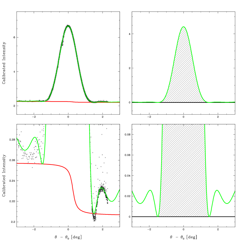
Figure 1: Example drift scan of Cas A, acquired with the 40-foot in L band. Top left: Measured intensity, in gain-calibration units, vs. angular position (black crosses), and best-fit source (green curve) plus background (red curve) functions. Data not collected near the final, locked-in elevation have already been excised. Bottom left: An expanded view, to better see the base of the best-fit source function and the best-fit background function. Right: Best-fit source function only (i.e., the background-subtracted best-fit model). The shaded area, divided by the source function’s peak value, $F_{m}$, defines $I_{m}$ (Equation 5).

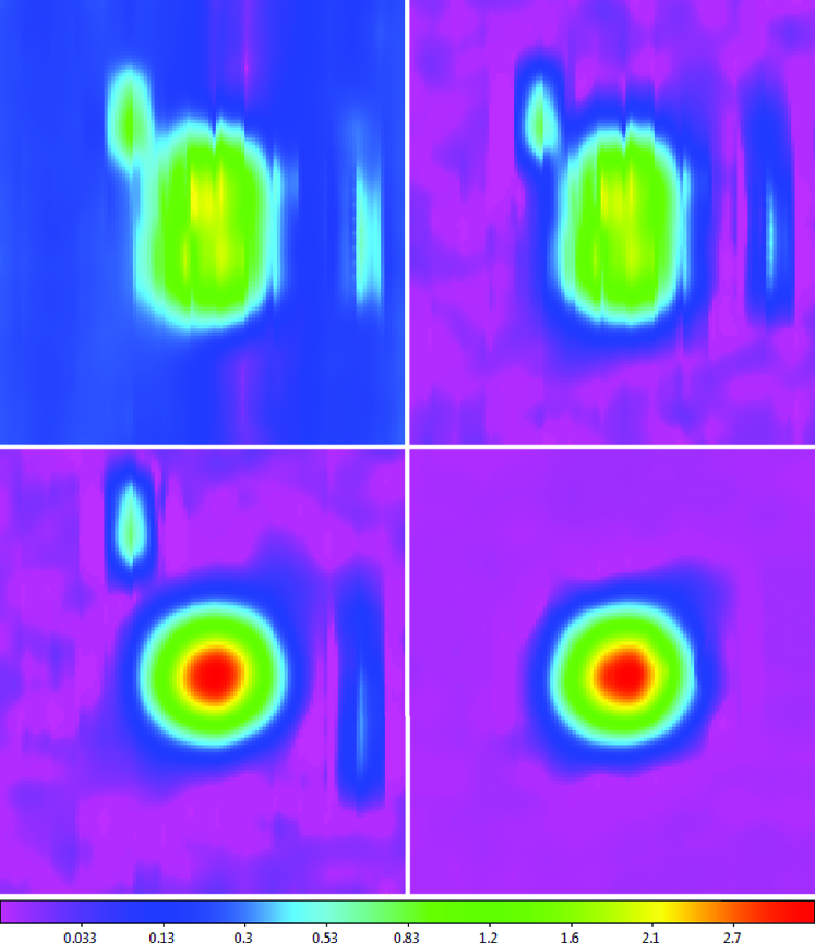
Figure 2: Example on-the-fly raster of Cas A, acquired with the 20-meter in X band. For all of our 20-meter observations, signal was integrated and read out every 0.2 beams (corresponding to every $7\arcmin$ in this, X-band case) along scans in declination (plotted here vertically), and scans were separated also by 0.2 beams, in right ascension (plotted here horizontally). In this case, we have zoomed into the central 5.7 beams $\times$ 5.7 beams, corresponding to $40\arcmin$ $\times$ $40\arcmin$. Top left: Gain-calibrated measurements. Top right: After background subtraction on the recommended, 6-beam scale. Bottom left: After time-delay correction, by which we mean that occasionally the clocks of the telescope’s separate coordinate and signal computers lose synchronization, which results in a hysteretic splitting of the source along the scan direction, prior to correction. Bottom right: After RFI cleaning, on the recommended, 0.8-beam scale. In all four panels, scale-weighted surface models have been fitted to the data about each pixel, for visualization. In the first three panels, a minimal scale is used, for maximal surface flexibility. In the fourth panel, the recommended, 1/3-beam (near-Nyquist) scale is used, and this is the final image. A non-linear color spectrum is used to emphasize fainter structures (units are dimensionless, with one corresponding to the noise diode). Details regarding the Skynet Robotic Telescope Network’s single-dish image-reduction pipeline will be available in Martin et al. (in prep.).

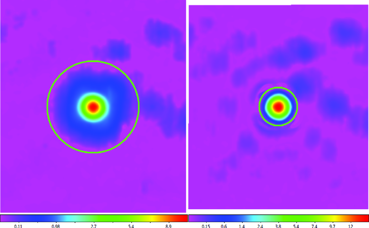
Figure 3: Example L-band images of Cas A, made with the 20-meter in 2014 (left) and 2016 (right). Each is 13.5 beams $\times$ 13.5 beams, corresponding to $10.1^{\circ}$ $\times$ $10.1^{\circ}$, with declination plotted vertically and right ascension plotted horizontally. A non-linear color spectrum is used to emphasize fainter structures (units are dimensionless, with one corresponding to the noise diode). The 2014 images are somewhat out of focus, requiring a larger aperture (green circle) for photometry. This had been corrected by 2016.

From each best fit, we calculated: (1) the measured peak intensity of the source:

$$F_{m}\equiv F_{s}(\theta_{0})=\left(\sum_{n=1}^{N}{a_{n}}\right)^{2}\,;$$ (4)

and (2) the integral of the measured source function, normalized to its peak value:

$$I_{m}\equiv\frac{1}{F_{m}}\int_{\theta_{0}-\Delta\theta}^{\theta_{0}+\Delta\theta}{F_{s}(\theta)d\theta}\,,$$ (5)

where the integration limits are the symmetric, first minima on either side of the source function (Figure 1, bottom right). In §3, we show that: (1) the Cas A-to-Cyg A flux-density ratio, $R_{m}$, depends not only on $F_{m,\mathrm{Cas}}$ and $F_{m,\mathrm{Cyg}}$, but also on $I^{2}_{m,\mathrm{Cas}}$ and $I^{2}_{m,\mathrm{Cyg}}$; and (2) $I^{2}_{m,\mathrm{Cas}}$ and $I^{2}_{m,\mathrm{Cyg}}$ can also be used to account for small errors in pointing and differences in focus, at least in part.

We list these ratios, $R_{m}$, and their corresponding values of $I^{2}_{m,\mathrm{Cas}}$ and $I^{2}_{m,\mathrm{Cyg}}$, in Table 2, for all same-week combinations of our Cas A and Cyg A measurements. For most years, we have only one Cyg A measurement, having made other observations during Cyg A’s transit time the rest of the week. For years where we have two Cyg A measurements, and three Cas A measurements, we assigned each ratio a weight of $2/3$, given redundancy of information in the six possible combinations. In total, we obtained 47 (41 non-redundant) L-band measurements of $R_{m}$ with the 40-foot over a 20-year period.

Table 3: Summary of GBO 20-meter L- and X-band observations.

Dates	Band	Source	Number of Observations
10 – 14 Jul 2014	L	Cas A	24
10 – 14 Jul 2014	L	Cyg A	24
17 Jul – 5 Aug 2014	X	Cas A	31
17 Jul – 5 Aug 2014	X	Cyg A	30
24 – 29 Sep 2016	L	Cas A	20
24 – 29 Sep 2016	L	Cyg A	23
6 – 8 Jan 2017	L	Cas A	23
5 – 8 Jan 2017	L	Cyg A	25
5 – 8 Jan 2017	L	Tau A	23
5 – 8 Jan 2017	L	Vir A	24

2.3 GBO 20-meter

In 2014, 2016, and 2017, we observed different combinations of Cas A, Cyg A, Tau A, and Vir A in different combinations of L (centered at 1395 MHz) and X (centered at 9000 MHz) bands using GBO’s 20-meter telescope (see Table 3). The 20-meter had recently been refurbished and integrated into the Skynet Robotic Telescope Network (Martin et al., in prep.). We submitted each observation through Skynet’s web-based user interface, after which they were automatically scheduled and completed. Each L-band observation consisted of a 13.5-beam $\times$ 13.5-beam on-the-fly raster, with 0.2-beam spacing between measurements, both along and between scans, and at a telescope slew speed of 0.5^∘/s took 23.0 minutes to complete. Each X-band observation consisted of an 18-beam $\times$ 18-beam on-the-fly raster, also with 0.2-beam spacing between measurements, and at a telescope slew speed of 0.3^∘/s took 10.5 minutes to complete. In total, 247 observations were completed.

Each observation was gain calibrated, background subtracted, time-delay corrected, RFI cleaned, and surface modeled using Skynet’s single-dish radio telescope image-reduction pipeline (Martin et al., in prep.; see Figure 2). We then photometered each image using 3- and 1.5-beam diameter apertures for the 2014 L- and X-band images, respectively, and using 1.25-beam diameter apertures for the 2016 and 2017 L-band images (focus had been improved for the later L-band images; see Figure 3).

We determined flux-density ratios by pairing each Cas A, Tau A, or Vir A measurement with its closest-in-time Cyg A measurement, and by pairing each Cyg A measurement with its closest-in-time Cas A, Tau A, or Vir A measurement. We then measured the mean and the uncertainty in the mean for each of these (six; see Table 4) collections of ratios, after rejecting outliers using Robust Chauvenet Rejection (RCR; Maples et al. 2017). More outliers were found with the Tau A and Vir A ratios than with the Cas A ratios, because, being on the other side of the sky than Cyg A, these pairs were generally observed with a greater separation in time. The 2017 Cas A ratios, however, were an exception, in that observations of Cyg A began a full day before observations of Cas A.

Table 4: GBO 20-meter L- and X-band flux-density ratio measurements, with respect to Cyg A.

Mean Epoch	Band	Source	Number of Ratios	Number Rejected	$R_{m}$
2014.53	L	Cas A	48	3	$1.123\pm 0.019$
2014.58	X	Cas A	61	0	$2.46\pm 0.19$
2016.74	L	Cas A	43	1	$1.115\pm 0.021$
2017.02	L	Cas A	48	16	$1.103\pm 0.021$
2017.02	L	Tau A	48	11	$0.529\pm 0.012$
2017.02	L	Vir A	49	17	$0.1370\pm 0.0015$

3 GBO Models and Fits

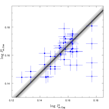
Figure 4: Measured values of the square of the integral of the peak-normalized source function from Table 1, plotted $\log\mbox{$I^{2}_{m,\mathrm{Cas}}$}$ vs. $\log\mbox{$I^{2}_{m,\mathrm{Cyg}}$}$. The line is the best fit of Equation 7 to these, weighted data. Open circles have been rejected using Robust Chauvenet Rejection (RCR; Maples et al. 2017), and correspond to pairs of measurements that likely suffer from significantly different pointing errors; they do not contribute to the fit. The shaded regions show the 1-, 2-, and 3-$\sigma$ statistical uncertainty in the best-fit value of $\log\beta$. The uncapped error bars show the best-fit 1-$\sigma$ sample scatter, which in this case is two-dimensional (see Trotter 2011, or Reichart 2001).

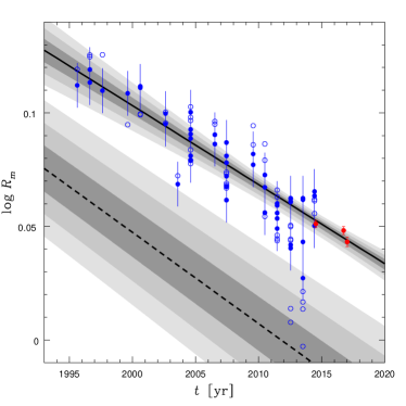
Figure 5: 23 years of GBO 40-foot (blue) and 20-meter (red) L-band Cas A-to-Cyg A flux-density ratios vs. time, and best-fit model (solid line). Open circles are measured values. Filled circles are after subtracting off the best-fit third and fourth terms of Equation 12, which account for imperfect pointing and non-constant focus of the 40-foot telescope. The shaded regions show the 1-, 2-, and 3-$\sigma$ statistical uncertainty in the best-fit values of $\log F_{0}$ and $m_{\nu_{0}}$. The uncapped error bars show the best-fit 1-$\sigma$ sample scatter of the 40-foot measurements (that of the 20-meter measurements is almost negligible). The significantly lower dashed line and shaded regions are from the fitted spectral and temporal models of Baars et al. (1977).

3.1 GBO 40-foot Pointing-Error and Non-Constant Focus Models

From our first five years of GBO 40-foot observations, Reichart & Stephens (2000) found that the ratio of Cas A’s peak intensity to that of Cyg A, $\mbox{$F_{m,\mathrm{Cas}}$}/\mbox{$F_{m,\mathrm{Cyg}}$}$, was significantly greater than expected, given the fitted spectral and temporal models of Baars et al. (1977). In this section, we investigate if our 40-foot measurements could be biased high, due to (1) imperfect pointing of the telescope, and/or (2) non-constant focus of the telescope.

Imperfect Pointing: If during a drift scan the operator fails to zero-in on the true transit elevation of the source (§2.2), the peak intensity that we would then measure for that source would be underestimated. Consequently, our higher-than-expected Cas A-to-Cyg A peak-intensity ratios could, at least in theory, be due to systematically greater pointing errors when we observed Cyg A. However, we regard this as unlikely: Each year, our scans of Cyg A were taken by the same, most-experienced member of our team, while most (but not all) of our scans of Cas A were taken by first-time, student operators. Hence, if anything, we would expect our Cas A-to-Cyg A peak-intensity ratios to be biased low due to imperfect pointing, not high.

Non-Constant Focus: Changes in temperature between observations of Cas A and Cyg A, and/or elevation-dependent differences in how gravity pulls on the dish and the receiver and its support structure could, at least in theory, change the focus of the telescope. Non-ideal focus would result in a broader point-spread function, and consequently, a lower peak intensity. Hence, if the conditions under which we took our Cyg A observations were such that focus was systematically poorer than for our Cas A observations, this could also explain our higher-than-expected Cas A-to-Cyg A peak-intensity ratios. But again, we regard this as unlikely: At the time of year that we took our observations, between June and August, both Cyg A and Cas A transit the meridian at night, or early in the morning, within 3.4 hours of each other, when temperatures at GBO are fairly stable. Furthermore, both sources transit the meridian at similar, high elevations ($87^{\circ}$ for Cyg A and $69^{\circ}$ for Cas A), so we do not expect gravitational distortion of the telescope to differ significantly either.

Although we anticipate that neither of these effects, imperfect pointing and non-constant focus, can account for our higher-than-expected Cas A-to-Cyg A peak-intensity ratios, we still model both effects (1) to be sure, and (2) to ensure that our fits to these data (see §3.2, §5) are as accurate as possible. As we will see in these sections, these effects are indeed small, generally offsetting, and insufficient to explain the discrepancy with Baars et al. (1977).

Pointing-Error Model: Imperfect pointing has two effects: (1) The measured peak intensity is less than the true peak intensity ($F_{m}<F_{t}$); and (2) The measured peak-normalized source function is likely different from the true, or perfect-pointing, peak-normalized source function, resulting in $I_{m}^{2}\neq I_{t}^{2}$. We model the consequent correlation, between measured peak intensity and the square of the integral of the measured peak-normalized source function, to first order, since pointing errors, if not negligible, were at least small (§2.2):

$$\frac{F_{m}}{F_{t}}=\left({\frac{I^{2}_{m}}{I^{2}_{t}}}\right)^{\alpha}\,,$$ (6)

where $\alpha$ is determined empirically in §3.2 and §5.

Non-Constant Focus Model: Non-constant focus would imply that the 40-foot’s true, or perfect-pointing, peak-normalized source function differs between our observations of Cas A and Cyg A. If there is a systematic component to this, we take it to be small, and, as above, model it to first order:

$$\mbox{$I^{2}_{t,\mathrm{Cas}}$}=\beta\mbox{$I^{2}_{t,\mathrm{Cyg}}$}\,,$$ (7)

where $\beta$ is also determined empirically in §3.2 and §5. That said, we can place a prior on $\beta$, by fitting Equation 7 to our measured values, $I^{2}_{m,\mathrm{Cas}}$ and $I^{2}_{m,\mathrm{Cyg}}$. As can be seen in Figure 4, these values appear to have changed in concert from year to year. We find that that $\log\beta=0.0070\pm 0.0010$, with a best-fit sample scatter of 0.0059 dex. Consequently, in our upcoming fits to 40-foot data (see §3.2 and §5), we adopt a Gaussian prior in $\log\beta$, of mean 0.0070 and width 0.0010 dex.

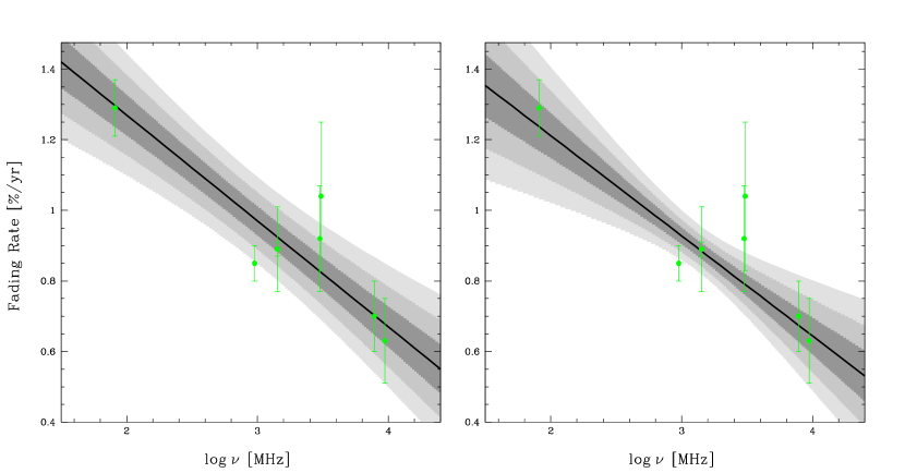
Figure 6: Fading-rate measurements from Table 1 of Baars et al. (1977), and best-fit models. The original result of Baars et al. (1977) is on the left; ours is on the right. The shaded regions show the 1-, 2- and 3-$\sigma$ statistical uncertainty in the best-fit values of $m_{\nu_{0}}$ and $m_{\Delta\log\nu}$. The best-fit sample scatter (at least in the case of our fit) is negligible. We were unable to reproduce the original result specifically, but do so generally.

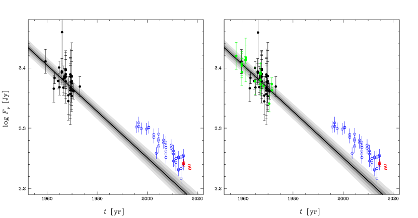
Figure 7: Absolute (black) and relative (green) measurements of the flux density of Cas A from Baars et al. (1977), and best-fit temporal models. Relative measurements have been multiplied by the best-fit spectral model of the reference source, and all measurements have been referenced to 1405 MHz using the best-fit spectral model of Cas A, for better visualization. Open circles are the GBO 40-foot (blue) and 20-meter (red) measurements from Figure 9, and are not included in these fits. The fit on the left is to just the plotted, absolute Cas A data. The fit on the right is a simultaneous fit to all Baars et al. (1977) flux-density data. Both fits are additionally constrained by the fading-rate priors of §4.1, from the right panel of Figure 6. The shaded regions show the 1-, 2-, and 3-$\sigma$ statistical uncertainty in the best-fit values of $\log F_{0}$, $a_{1}$, $a_{2}$, $a_{3}$, $m_{\nu_{0}}$, and $m_{\Delta\log\nu}$. The best-fit sample scatter is negligible. This confirms that the Baars et al. (1977) data do indeed imply a trend that undercuts our GBO data at later times (Figure 5).

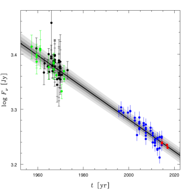
Figure 8: Absolute (black) and relative (green) measurements of the flux density of Cas A from Baars et al. (1977), our (also relative) GBO 40-foot (blue) and 20-meter (red) measurements, and our best-fit, one-segment temporal model of both epochs. Relative measurements have been multiplied by the best-fit spectral model of the reference source, and all measurements have been referenced to 1405 MHz using the best-fit spectral model of Cas A, for better visualization. 40-foot measurements have additionally been corrected for imperfect pointing and non-constant focus using the best-fit values of $\alpha$ and $\beta$, as in Figure 5, also for better visualization. The fading-rate priors of §4.1 apply only to the epoch of the Baars et al. (1977) data and consequently have not been included in this fit. The shaded regions show the 1-, 2-, and 3-$\sigma$ statistical uncertainty in the best-fit values of $\log F_{0}$, $a_{1}$, $a_{2}$, $a_{3}$, $m_{\nu_{0}}$, and $m_{\Delta\log\nu}$. The uncapped error bars show the best-fit 1-$\sigma$ sample scatter of the 40-foot measurements (that of the other measurements is negligible).

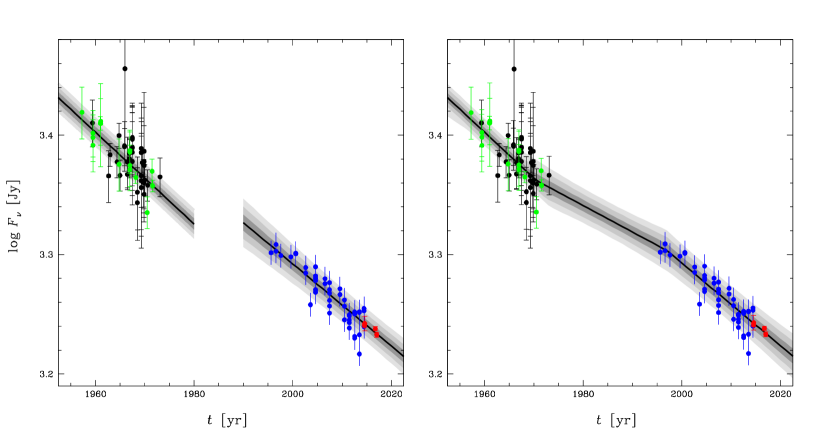
Figure 9: The same as Figure 8, but for our best-fit two-segment (left) and three-segment (right) temporal models. The fading-rate priors of §4.1 have been applied to the first segment of each model.

3.2 GBO 40-foot and 20-meter Model and Fit

Of course, it is not the ratio of Cas A’s and Cyg A’s peak intensities that we must model, but the ratio of their integrated intensities, which do not depend on the telescope’s precise pointing or focus, nor on the intrinsic size of the source. With the 20-meter, this is straightforward: We densely sample each source’s 2D distribution on the sky, and can reconstruct and integrate these distributions (§2.3). But with the 40-foot, we have only single, 1D slices through these 2D distributions (§2.2). However, if one assumes radial symmetry, or at least the same shape, if not the same size, for these sources’ 2D distributions, integrated intensity is then simply:

$$S_{t}\propto F_{t}I_{t}^{2}\,,$$ (8)

where subscript $t$ again refers to true, or perfect-pointing, values. Given this, we define the measured Cas A-to-Cyg A flux-density ratio analogously:

$$R_{m}=\frac{S_{m,\mathrm{Cas}}}{S_{m,\mathrm{Cyg}}}\equiv\frac{\mbox{$F_{m,\mathrm{Cas}}$}\mbox{$I^{2}_{m,\mathrm{Cas}}$}}{\mbox{$F_{m,\mathrm{Cyg}}$}\mbox{$I^{2}_{m,\mathrm{Cyg}}$}}\,.$$ (9)

These are the values that we list in Table 2. Note, Equation 9 reduces to $R_{m}=F_{m,\mathrm{Cas}}/F_{m,\mathrm{Cyg}}$ in the limit of perfect pointing and identical 2D distributions.

Substituting our pointing-error (Equation 6) and non-constant focus (Equation 7) models into Equation 9 yields:

$$R_{m}=\frac{\mbox{$F_{t,\mathrm{Cas}}$}\mbox{$I^{2}_{t,\mathrm{Cas}}$}}{\mbox{$F_{t,\mathrm{Cyg}}$}\mbox{$I^{2}_{t,\mathrm{Cyg}}$}}\left(\frac{\mbox{$I^{2}_{m,\mathrm{Cas}}$}}{\beta\mbox{$I^{2}_{m,\mathrm{Cyg}}$}}\right)^{\alpha+1}\equiv R_{t}\left(\frac{\mbox{$I^{2}_{m,\mathrm{Cas}}$}}{\beta\mbox{$I^{2}_{m,\mathrm{Cyg}}$}}\right)^{\alpha+1}\,,$$ (10)

where $R_{t}\equiv\mbox{$F_{t,\mathrm{Cas}}$}\mbox{$I^{2}_{t,\mathrm{Cas}}$}/\mbox{$F_{t,\mathrm{Cyg}}$}\mbox{$I^{2}_{t,\mathrm{Cyg}}$}$ is the true, or perfect-pointing, Cas A-to-Cyg A flux-density ratio at the time of the observations.

Given the size of Cyg A’s emitting region, Cyg A’s brightness should not change over the timescale of these observations. Consequently, the observed decrease in $R_{t}$ with time must be due to Cas A fading. In keeping with Baars et al. (1977), we model this fading exponentially:

$$R_{t}(t)=R_{0}e^{m_{\nu_{0}}(t-t_{0})}\,,$$ (11)

where $R_{0}\equiv R_{t}(t_{0})$; $t_{0}$ is a reference time, which in this paper we set equal to the weighted mean of whichever observations we are fitting to; and $m_{\nu_{0}}$ is the fading rate, in this case at $\nu_{0}=1405$ MHz. In units of percent per year, this is $-100\times\ln 10\times m_{\nu_{0}}$.

Substituting Equation 11 into Equation 10 and taking the logarithm of both sides yields:

$$\begin{split}\log R_{m}(t)=&\log R_{0}+m_{\nu_{0}}(t-t_{0})\\ &+(\alpha+1)\log\left({\frac{\mbox{$I^{2}_{m,\mathrm{Cas}}$}}{\mbox{$I^{2}_{m,\mathrm{Cyg}}$}}}\right)-(\alpha+1)\log\beta\,,\end{split}$$ (12)

where the first two terms model the normalization and fading of the flux-density ratio, respectively; the third term accounts for imperfect pointing of the telescope, for 40-foot data; and the fourth term accounts for systematic differences in focus between observations of Cas A and Cyg A, again for 40-foot data. Equation 12 can also, and simultaneously, be fitted to our 20-meter L-band Cas A-to-Cyg A flux-density ratios (Table 4), by dropping the last two terms for these data.

We plot our best fit of Equation 12 to all 23 years of GBO 40-foot and 20-meter L-band measurements in Figure 5. We find that $\log R_{0}=0.0557^{+0.0011}_{-0.0019}$ (at $t_{0}\equiv 2013.65$), $m_{\nu_{0}}=-0.00348^{+0.00022}_{-0.00023}$ (corresponding to $0.802^{+0.053}_{-0.050}$ %/yr), $\alpha=0.64\pm 0.15$, and $\log\beta=0.00754^{+0.00090}_{-0.00089}$, with best-fit sample scatters of 0.0099 dex for the 40-foot data and 0.0014 dex for the 20-meter data.

The fitted pointing-error and non-constant focus “correction” terms in Equation 12 are, as expected, small, but not negligible. The mean pointing-error correction is $0.00774\pm 0.00073$ dex, or $1.80\pm 0.17$ %. This suggests that, on average, our pointing was a bit better for Cyg A than for Cas A, as expected (§3.1). The non-constant focus correction is $-0.0123\pm 0.0019$ dex, or $-2.80\pm 0.42$ % (this uncertainty is 44% anti-correlated with the uncertainty in the mean pointing-error correction). This suggests that the 40-foot’s focus was a bit worse when observing Cas A than when observing Cyg A, for either of the reasons postulated in §3.1. The former correction, visibly, accounts for some of the scatter of the data about the best-fit model (Figure 5), and raises the best-fit model. The latter correction lowers the best-fit model, to be in accordance with the 20-meter data, although $\log\beta$ is also constrained by the prior that we were able to place on it in §3.1. The sum of these corrections is $-0.0046\pm 0.0015$ dex, or $-1.05\pm 0.35$ %, which falls significantly short of the roughly $-0.06\pm 0.01$ dex, or $-15\pm 2$ % correction that would be required to explain the discrepancy with the fitted spectral and temporal models of Baars et al. (1977), first identified by Reichart & Stephens (2000) (Figure 5). Furthermore, the 20-meter measurements, which are not subject to these corrections, confirm this discrepancy.

4 Models and Fits to the Baars et al. (1977) Data

Now that we have established that Cas A is, and has been since at least the mid-1990s, significantly brighter than expected, given the fitted spectral and temporal models of Baars et al. (1977), at least in L band, two likely explanations remain: (1) Cas A rebrightened sometime between the end of the Baars et al. (1977) observations and the beginning of our GBO observations, so between the mid-1970s and mid-1990s, after which it resumed fading; or (2) the fitted spectral and/or temporal models of Baars et al. (1977) are erroneous. Given this, and given the importance of these fitted models for flux-density calibration in radio astronomy, we now re-analyze the original Baars et al. (1977) data.

4.1 Temporal Model and Fit

We begin by fitting the same, frequency-dependent fading-rate model to the same fading-rate measurements that Baars et al. (1977) did. The fading-rate model is given by:

$$-\frac{100}{F_{\nu}}\frac{dF_{\nu}}{dt}=m_{\nu_{0}}+m_{\Delta\log\nu}\log\left(\frac{\nu}{\nu_{0}}\right)\,,$$ (13)

where we have decided to normalize the function at the weighted mean of the data’s $\log\nu$ values (corresponding to $\nu_{0}\equiv 1315$ MHz), instead of at 1 GHz. The fading-rate measurements are from Table 1 of Baars et al. (1977).

We plot our best fit of Equation 13 to these measurements in the right panel of Figure 6. We find that $m_{\nu_{0}}=0.894\pm 0.021$ %/yr and $m_{\Delta\log\nu}=-0.284\pm 0.053$ %/yr, with a best-fit sample scatter of zero. This differs from the original result of Baars et al. (1977) (left panel), which has marginally different best-fit values, but significantly different uncertainties in these best-fit values: Baars et al. (1977) appears to have overstated the uncertainty in the best-fit model around 1 GHz, and understated it below $\approx$100 MHz. Despite this, our fitted temporal models are sufficiently similar that this is unlikely to be the source of the discrepancy in Figure 5.

4.2 Spectral Model and Fits

Baars et al. (1977) used their best-fit temporal model to reference all of their measurements to epoch 1965, after which they fitted their spectral model to these “corrected” measurements. Generally, this is a poor modeling practice, in that it is seldom clear how all of the various uncertainties propagate. Instead, we fit our spectral and temporal models simultaneously (§2.1), adopting the results of the previous section as priors. Otherwise, our only difference is that we use a slightly different spectral model: Where Baars et al. (1977) used piecewise linear and quadratic models, we use a third-order polynomial model over the entire, 22 MHz to 22 GHz, spectral range. Our combined spectral and temporal model is then given by:

$$\begin{split}\log F_{m}(\nu,t)=&\log F_{0}+a_{1}\log\left(\frac{\nu}{\nu_{\mathrm{Cas}}}\right)\\ &+a_{2}\left[\log\left(\frac{\nu}{\nu_{\mathrm{Cas}}}\right)\right]^{2}+a_{3}\left[\log\left(\frac{\nu}{\nu_{\mathrm{Cas}}}\right)\right]^{3}\\ &+\left[m_{\nu_{0}}+m_{\Delta\log\nu}\log\left(\frac{\nu}{\nu_{0}}\right)\right](t-t_{0})\,,\end{split}$$ (14)

where the first term is the normalization; the next three terms are our spectral model, normalized at the weighted mean of the data’s $\log\nu$ values; and the last term is our frequency-dependent temporal model, where, a priori, we take $m_{\nu_{0}}$ to be distributed as a Gaussian of mean 0.894 %/yr and width 0.021 %/yr, $m_{\Delta\log\nu}$ to be distributed as a Gaussian of mean -0.284 %/yr and width 0.053 %/yr, and $\nu_{0}\equiv 1315$ MHz (§4.1).

Table 5: Best-fit parameter values and 1-$\sigma$ statistical uncertainties in these values for our favored, three-segment model.

Cas A Segment Specific
Parameter	Segment 1	Segment 2	Segment 3
$\log F_{0}$	$3.3731\pm 0.0037$	$3.3173\pm 0.0047$	$3.2530^{+0.0051}_{-0.0050}$
$m_{\nu_{0}}$	$-0.003884^{+0.000092}_{-0.000093}$	$-0.00227\pm 0.00024$	$-0.00350^{+0.00022}_{-0.00025}$
	($0.894\pm 0.021$ %/yr)	($0.522^{+0.056}_{-0.054}$ %/yr)	($0.806^{+0.058}_{-0.050}$ %/yr)
reference time	1963.9	1983.8	2006.9

Source Specific
Parameter	Cas A	Cyg A	Tau A	Vir A
$\log F_{0}$	segment specific	$3.1861^{+0.0046}_{-0.0047}$	$2.9083^{+0.0044}_{-0.0045}$	$2.3070^{+0.0045}_{-0.0046}$
$a_{1}$	$-0.732^{+0.011}_{-0.010}$	$-1.038\pm 0.011$	$-0.226^{+0.014}_{-0.013}$	$-0.876\pm 0.017$
$a_{2}$	$-0.0094^{+0.0058}_{-0.0059}$	$-0.1457^{+0.0075}_{-0.0077}$	$-0.0113^{+0.0081}_{-0.0083}$	$-0.047^{+0.031}_{-0.033}$
$a_{3}$	$0.0053\pm 0.0058$	$0.0170^{+0.0075}_{-0.0076}$	$-0.0275^{+0.0077}_{-0.0079}$	$0.073^{+0.030}_{-0.029}$
reference frequency	1477 MHz	1416 MHz	1569 MHz	1482 MHz
$m_{\nu_{0}}$	segment specific	–	$-0.00044^{+0.00019}_{-0.00018}$	–
			($0.102^{+0.042}_{-0.043}$ %/yr)
reference time	segment specific	–	2009.05	–
$m_{\Delta\log\nu}$	$0.00124\pm 0.00018$	–	–	–
	($-0.286\pm 0.042$ %/yr)
reference frequency	1315 MHz	–	–	–
reference time	2005.64	–	–	–

Telescope Specific
Parameter	40-foot	All Others
$\alpha$	$0.64^{+0.16}_{-0.15}$	–
$\beta$	$0.00757^{+0.00091}_{-0.00089}$	–
scatter	$0.0099$	$0$

In the left panel of Figure 7, we fit Equation 14 to the exact same measurements that Baars et al. (1977) did, the absolute measurements of Cas A listed in their Table 2. In the right panel, we expand upon this by additionally fitting to all of their relative measurements of Cas A, which are respect to Vir A. This requires simultaneously fitting to Vir A, and as some of these measurements are relative to Cyg A and Tau A, this requires simultaneously fitting to all four sources. For this, we adopt the same, third-order polynomial spectral model for each source, but with independent parameters and normalization reference frequencies. In either case, we confirm that the Baars et al. (1977) data do indeed imply a trend that undercuts our GBO data at later times, albeit by a marginally smaller amount, but also at a greater level of significance, compared to the original result (Figure 5).

5 Combined Models and Fits

We have now established that neither our more recent, GBO measurements (§3) nor the original, fitted spectral and temporal models of Baars et al. (1977) (§4) have misdirected us (although we were not able to reproduce the latter exactly, and with more powerful statistical and computing techniques, have been able to improve on these models, especially within certain frequency ranges; see below). Consequently, we conclude that Cas A rebrightened, or at least faded at a much slower rate, between the end of the Baars et al. (1977) observations and the beginning of our GBO observations (§4).

In this section, we begin by modeling the average fading rate of Cas A between the late 1950s and late 2010s, by ignoring the fading-rate priors of §4.1, which clearly apply only to the epoch of the Baars et al. (1977) data. We then reintroduce these priors, and model the fading of Cas A in two ways: (1) assuming a rebrightening event between the last Baars et al. (1977) observation and our first GBO observation; and (2) assuming a period of much slower fading between these epochs.

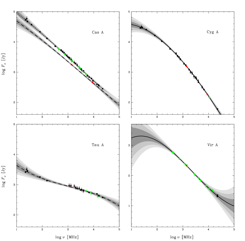
Figure 10: Our best-fit spectral models (specifically, corresponding to the best-fit three-segment temporal model of Figure 9). The data are color-coded as in Figures 8 and 9. Note, however, that we have not plotted the GBO 40-foot data here, for greater clarity at this frequency. Relative measurements (green and red) have again been multiplied by the best-fit spectral model of the reference source, and (1) the Baars et al. (1977) Cas A measurements have been referenced to 1965 (dotted curve), (2) our GBO Cas A measurements have been referenced to 2015 (dashed curve), and (3) all Tau A measurements have been referenced to 2015 (dashed curve) using the best-fit temporal models of Cas A and Tau A, respectively, for better visualization. The shaded regions show the 1-, 2-, and 3-$\sigma$ statistical uncertainty in the best-fit values of $\log F_{0}$, $a_{1}$, $a_{2}$, $a_{3}$, and, when applicable, $m_{\nu_{0}}$, and $m_{\Delta\log\nu}$. The best-fit sample scatter of all but the 40-foot measurements is negligible.

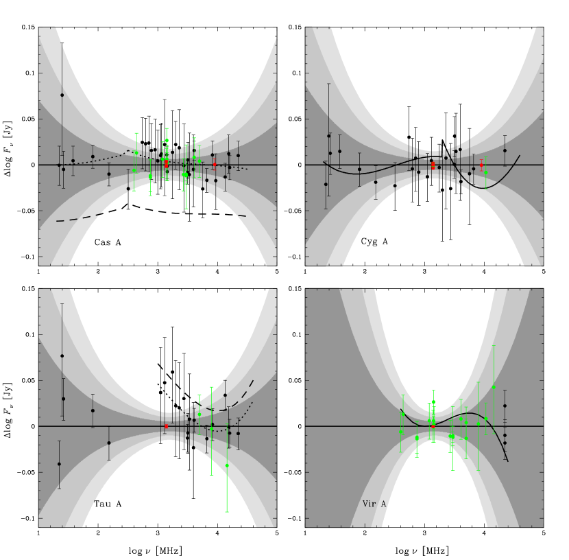
Figure 11: Difference between the original, best-fit spectral models of Baars et al. (1977) and our updated and improved best-fit spectral models (Figure 10). The Baars et al. (1977) Cas A and Tau A models have been referenced to 1965 (dotted) and 2015 (dashed), respectively. Our Cas A and Tau A models have been referenced to 2015. Clearly, Baars et al. (1977) overpredicted the fading of Cas A, and appear to have also underpredicted (specifically, set to zero) the fading of Tau A. But even the 1965 versions of these curves differ by up to $\approx$6% – $\approx$11% in the couple- to many-GHz range of some of these spectra (Cyg A and Tau A in particular).

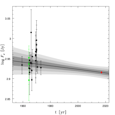
Figure 12: The same as Figure 8, but for Tau A. The fading of Tau A appears to be measurable over this timescale.

For both of these models, we fit to all data (Cas A, Cyg A, Tau A, and Vir A) simultaneously, as we did in §4.2. Given the longer timescale over which these observations were made, we also permit Tau A to fade (neither Cyg A nor Vir A should). However, we do not have enough late-time data to measure if this fading also has a frequency dependence, so for Tau A, we simply measure its fading rate in L band. Furthermore, we do not have enough late-time data to measure if the frequency dependence of Cas A’s fading rate is also changing, so we take it to be constant across all epochs.

5.1 Average Fading Model and Fit

Our fading-rate priors (§4.1) derive from eight fading-rate measurements. On average, these measurements were made over $12.9\pm 4.4$ year spans of time, beginning in $1959.1\pm 4.8$ and ending in $1972\pm 2.1$. As such, these priors are germane really only to this relatively brief period, which matches the epoch of the rest of the Baars et al. (1977) data almost perfectly. So, if we wish to characterize Cas A with a single fading rate, representative of all of the epochs for which we have data, we should not necessarily bind ourselves with these priors. Dropping them for this fit only yields: $\log(F_{0}/1~{}\mathrm{Jy})=3.2494^{+0.0041}_{-0.0042}$ (at $t_{0}=2005.64$), $m_{\nu_{0}}=0.663\pm 0.019$ %/yr, $m_{\Delta\log\nu}=-0.317\pm 0.067$ %/yr, and a best-fit sample scatter for all but the 40-foot data (i.e., for all data with measured uncertainties) of zero (see Figure 8). At 1405 MHz, this corresponds to a fading rate of $0.670\pm 0.019$ %/yr, which is consistent with our initial finding of $0.62\pm 0.12$ %/yr (Reichart & Stephens 2000). This is also consistent with the finding of Vinyaikin (2007a), who measured a fading rate of $0.67\pm 0.04$ %/yr between 1977 and 2004 at the nearby frequency of 927 MHz using the 10-meter diameter radio telescope at Staraya Pustyn’ Radio Astronomy Observatory in Russia. However, all of these measurements are inconsistent with the fading rate measured during the epoch of the Baars et al. (1977) data: $0.93\pm 0.04$ %/yr at 1405 MHz as measured by Baars et al. (1977), or $0.886\pm 0.021$ %/yr at 1405 MHz as we have remeasured it, in §4.1.

5.2 Rebrightening Models and Fits

Next, we fit two- and three-segment models to the same data. In the case of the two-segment model, we fit one segment to the Baars et al. (1977) data, one segment to our GBO data, and we assume that an, unmodeled, rebrightening event took place between these segments. In the case of the three-segment model, we assume a less-dramatic rebrightening, consisting merely of a period of slower fading, between two faster-fading segments. In both cases, we include the fading-rate priors of §4.1, applying them to the first segment only. We plot our best-fit two- and three-segment models in the left and right panels of Figure 9, respectively.

Compared to a one-segment model with the fading-rate priors also applied, these two- and three-segment, rebrightening models are favored at the 6.8$\sigma$ ($\Delta\chi^{2}=49.8$, $\Delta\nu=2$) and 6.3$\sigma$ ($\Delta\chi^{2}=50.4$, $\Delta\nu=4$) credible levels, respectively.

Vinyaikin (2006), Vinyaikin (2007a), and Vinyaikin (2014) (and references therein) observed Cas A and Cyg A between the two primary epochs considered in this paper, and at a variety of frequencies. We did not include these data in our analysis, because the scatter of these data (compared to their measured uncertainties) suggests that systematics might be an issue, and we do not know enough about these telescopes to model possible systematics (e.g., as we did in §3). However, these data are still useful to us in that they show no evidence of a sudden rebrightening, but are generally consistent with monotonic fading, which favors our three-segment model over our two-segment model. We present best-fit parameter values and uncertainties for this, 27-parameter, model in Table 5.

Both of our rebrightening models, as well as the one-segment model from §5.1, result in nearly identical fitted spectral models. We plot these for our favored, three-segment model, and for all four sources, in Figure 10 (also, see Perley & Butler 2016 for an independent analysis).

To examine the quality of the original, fitted spectral models of Baars et al. (1977), we plot their difference from our updated and improved versions in Figure 11. As we have already established, Baars et al. (1977) overpredicted the fading of Cas A, and consequently their Cas A spectrum is now too low. Conversely, they assumed no fading for Tau A, and consequently their Tau A spectrum now appears to be too high (see below).

However, even if one restricts oneself to an apples-to-apples comparison at epoch 1965, there are still significant differences. In particular, the Baars et al. (1977) Cyg A spectrum is (1) discontinuous, (2) significantly high (up to $\approx$7%) in the few-GHz range, and (3) significantly low (up to $\approx$6%) in the many-GHz range. And the Baars et al. (1977) Tau A spectrum is significantly high (up to $\approx$11%) in the couple-GHz range. These differences are much larger than the $\approx$2% accuracy quoted by Baars et al. (1977).

Finally, for Tau A, we measure a fading rate of $m_{\nu_{0}}=0.102^{+0.042}_{-0.043}$ %/yr in L band (see Figure 12). Vinyaikin (2007b) found a similar result: $0.18\pm 0.10$ %/yr, from observations made between 1977 and 2000 at 927 MHz.

For all of our fitted models, we have made every effort to select reasonable reference frequencies and times, in an attempt to minimize correlations between the fitted parameters. Given this, one may approximate the positive and negative 1-$\sigma$ uncertainties in any of our best-fit spectral and temporal models, at any frequency and time, by taking the square root of the following function:

$$\begin{split}\sigma_{\log F_{m}}^{2}(\nu,t)\approx\,\,&\sigma_{\log F_{0}}^{2}+\sigma_{a_{1}}^{2}\left[\log\left(\frac{\nu}{\nu_{\mathrm{source}}}\right)\right]^{2}\\ &+\sigma_{a_{2}}^{2}\left[\log\left(\frac{\nu}{\nu_{\mathrm{source}}}\right)\right]^{4}+\sigma_{a_{3}}^{2}\left[\log\left(\frac{\nu}{\nu_{\mathrm{source}}}\right)\right]^{6}\\ &+\sigma_{m_{\nu_{0}}}^{2}(t-t_{\mathrm{segment}})^{2}\\ &+\sigma_{m_{\Delta\log\nu}}^{2}\left[\log\left(\frac{\nu}{\nu_{0}}\right)\right]^{2}(t-t_{\mathrm{source}})^{2}+\sigma_{\mathrm{scatter}}^{2}\,,\end{split}$$ (15)

where $\sigma_{X}$ is the positive or negative 1-$\sigma$ statistical uncertainty, respectively, in the best-fit value of parameter $X$; the two temporal terms are only for Cas A and Tau A, and in the case of Tau A, the reference time $t_{\mathrm{segment}}=t_{\mathrm{source}}$; and for all four sources, the best-fit scatter $\sigma_{\mathrm{scatter}}=0$ in all of these fits (e.g., Table 5).

6 Conclusions

The fading of Cas A appears to be more complicated than originally measured, with the remnant fading quickly between the late 1940s and late 1960s/early 1970s ($0.886\pm 0.021$ %/yr in L band), then more slowly until the mid- to late 1990s ($0.516^{+0.056}_{-0.054}$ %/yr in L band), and then quickly again until at least the late 2010s ($0.798^{+0.058}_{-0.050}$ %/yr in L band; §5.2). Whether Cas A will continue to fade at this rate, or over longer timescales will more closely adhere to the average that we measured between the late 1950s and late 2010s ($0.654\pm 0.019$ %/yr in L band; §5.1) is unknown. Consequently, care should be taken if calibrating against Cas A, or Tau A for that matter, although Tau A is fading much more slowly, and consequently should remain reasonable as a calibrator longer.

Furthermore, we have identified potential weaknesses in the absolute spectral calibrations provided by Baars et al. (1977), particularly for Cyg A and Tau A in the couple- to many-GHz range, not due to measurement errors, but due, perhaps, to statistical and computing limitations at the time (§5.2). We have updated and improved these calibrations, for Cas A, Cyg A, Tau A, and Vir A, and have provided a better way to characterize the uncertainty in these calibrations, as a function of frequency, and, in the case of Cas A and Tau A, as a function of time.

This work can be improved upon in the future with additional measurements of Cas A at other frequencies, to see if the frequency dependence of its fading rate is also changing, and with additional measurements of Tau A, both at L band and at other frequencies, to measure the frequency dependence of its fading rate.

References

- Baars & Hartsuijker (1972) Baars, J. W. M., Hartsuijker, A. P. 1972, AA, 17, 172
- Baars et al. (1977) Baars, J. W. M., Genzel, R., Pauliny-Toth, I. I. K., & Witzel, A. 1977, A&A, 61, 99
- Baars, Mezger, & Wendker (1965) Baars, J. W. M., Mezger, P. G., & Wendker, H. 1965, ApJ, 142, 122
- Dent, Aller, & Olsen (1974) Dent, W. A., Aller, H. D., & Olsen, E. T. 1974, ApJ, 188, L11
- Erickson & Perley (1975) Erickson, W. C., & Perley, R. A. 1975, ApJ, 200, L83
- Jansesen, Golden, & Welch (1974) Janssen, M. A., Golden, L. M., & Welch, W. J. 1974, A&A, 33, 373
- Kellermann et al. (1981) Kellermann, K. I., Downes, A. J. B., Pauliny-Toth, I. I. K., Preuss, E., Shaffer, D. B. & Witzel, A. 1981, A&A, 97, L1
- Maples et al. (2017) Maples, M. P., Reichart, D. E., Berger, T. A., Trotter, A. S., Martin, J. R., Paggen, M. L., Joyner, R. E., Salemi, C. P., & Dutton, D. A. 2017, ApJS, submitted
- Perley & Butler (2016) Perley, R. A., & Butler, B. J. 2016, ApJS, submitted (arxiv:1609.05940)
- Read (1977a) Read, P. L. 1977a, MNRAS, 178, 259
- Read (1977b) Read, P. L. 1977b, MNRAS, 181, 63P
- Reichart (2001) Reichart, D. E. 2001, ApJ, 553, 235
- Reichart & Stephens (2000) Reichart, D. E. & Stephens, A. W. 2000, ApJ, 537, 904
- Shklovskii (1960) Shklovskii, I. S. 1960, SvA, 4, 243
- Trotter (2011) Trotter, A. S. 2011, The Gamma-Ray Burst Afterglow Modeling Project: Foundational Statistics and Absorption & Extinction Models, PhD dissertation, University of North Carolina at Chapel Hill (Chapel Hill, NC: ProQuest/UMI)